

1. Introduction
The Leidenfrost effect was discovered in 1756 by Johann Gottlob Leidenfrost (Leidenfrost Reference Leidenfrost1756), who observed that a drop falling onto a spoon heated over glowing coals did not adhere to the spoon but instead exhibited remarkable non-wettability and mobility (Quéré Reference Quéré2013). This phenomenon is highly dependent on the temperature of the solid substrate. Only when the temperature exceeds a critical threshold, known as the Leidenfrost temperature, can the evaporation rate generates a thin vapour film beneath the drop, causing it to levitate (Quéré Reference Quéré2013). On solid substrates, the Leidenfrost temperature is influenced by both the wettability (Zhong & Guo Reference Zhong and Guo2017) and the morphology of the solid surface (Hidalgo-Caballero, Escobar-Ortega & Pacheco-Vázquez Reference Hidalgo-Caballero, Escobar-Ortega and Pacheco-Vázquez2016; Wakata et al. Reference Wakata, Zhu, Chen, Lyu, Lohse, Chao and Sun2023), ranging from
 $130^{\,\circ}$
C on silicon superhydrophobic surfaces featuring nanosize textures (Bourrianne, Lv & Quere Reference Bourrianne, Lv and Quéré2019) to a typical value of
 $210^{\,\circ}$
C on a smooth hydrophilic silicon wafer (Bourrianne et al. Reference Bourrianne, Lv and Quéré2019) and reaching as high as
 $1150^{\,\circ}$
C on well-designed structured thermal armour (Jiang et al. Reference Jiang2022). On liquid substates, Leidenfrost drops can levitate at extremely low superheat level (the excess of substrate temperature above the drop’s boiling point), as low as
 $1^{\,\circ}$
C (Maquet et al. Reference Maquet, Sobac, Darbois-Texier, Duchesne, Brandenbourger, Rednikov, Colinet and Dorbolo2016). The Leidenfrost effect has attracted significant interest due to its complex interfacial and fluid dynamics phenomena (Quéré Reference Quéré2013), as well as its applications in engineering, particularly in thermal management (Jiang et al. Reference Jiang2022; Edalatpour, Colón & Boreyko Reference Edalatpour, Colón and Boreyko2023). Among the various aspects of the Leidenfrost effect, a key concern for researchers is ‘chimney instability’ as it plays a critical role in determining the maximum size range for which the drop shape remains stable. Additionally, promoting chimney instability can help disrupt the vapour layer and enhance internal convection in the liquid, thereby improving heat transfer performance (Singh & Sharma Reference Singh and Sharma2021).
When the radius of the Leidenfrost drop exceeds the capillary length
 ${l}_{{c}} = (\gamma /\rho g){}^{1/2}$
(2.5 mm for boiling water), gravitational force dominates over capillary force, causing it to transition from a spherical shape to a puddle (Biance, Clanet & Quere Reference Biance, Clanet and Quéré2003). Here,
 $\gamma$
and
 $\rho$
denote the surface tension and mass density of water, respectively, and g represents gravitational acceleration. The increase of drop size not only impacts the upper part of the drop but also contributes to an increase in the thickness of the vapour layer beneath the Leidenfrost drop (Burton et al. Reference Burton, Sharpe, van der Veen, Franco and Nagel2012; Sobac et al. Reference Sobac, Rednikov, Dorbolo and Colinet2014), until a phenomenon known as ‘chimney instability’ occurs. Experimental observations have shown that when the radius of the drop exceeds a critical radius
 ${r}_{{c}}^{*}$
= 4.0
 $\pm$
0.2 (non-dimensionalised by
 ${l}_{{c}}$
), a vapour bubble within the drop rises due to buoyancy and bursts upon reaching the apex of the upper liquid–air interface (Biance et al. Reference Biance, Clanet and Quéré2003), resembling a ‘chimney’. For larger drops, multiple chimneys may form. Experiments conducted in a large centrifuge facility to simulate varying gravity conditions have demonstrated that the average spacing between adjacent chimneys scales linearly with the capillary length (Maquet et al. Reference Maquet, Brandenbourger, Sobac, Biance, Colinet and Dorbolo2015). The formation of chimneys represents an abrupt morphological change in Leidenfrost drops and was initially attributed to Rayleigh–Taylor instability, where a heavy liquid drop is supported by a lighter vapour layer (Biance et al. Reference Biance, Clanet and Quéré2003). By introducing a sinusoidal perturbation to the bottom liquid–vapour interface of the drop, pressure perturbation analysis yields a theoretical value of
 ${r}_{{c}}^{*}$
= 3.85, which is consistent with experimental results (Biance et al. Reference Biance, Clanet and Quéré2003). Duchemin, Lister & Lange (Reference Duchemin, Lister and Lange2005) proposed a numerical methodology for solving the governing equations describing the profile of drops levitated by a lubrication gas cushion. This approach provides a precise prediction of the gas flow, indicating that chimney instability emerges when the solution becomes unphysical – specifically, when the lower interface penetrates the upper surface of the drop. Similarly, Snoeijer, Brunet & Eggers (Reference Snoeijer, Brunet and Eggers2009) performed asymptotic analyses of drop profiles and derived a full theoretical solution for
 ${r}_{{c}}^{*}$
, concluding that
 ${r}_{{c}}^{*}$
= 3.95 for typical experimental flow rates. Later, Sobac et al. (Reference Sobac, Rednikov, Dorbolo and Colinet2014) established a comprehensive model linking gas flow to evaporation, which accurately describes the shape of Leidenfrost drops. The numerical results of this model reveal a breakdown of the lubrication regime as the dimensionless drop radius approaches 4.0, signalling the onset of chimney instability. Furthermore, this model has also been applied to investigate the vapour layer profile of Leidenfrost drops under varying gravity conditions (Maquet et al. Reference Maquet, Brandenbourger, Sobac, Biance, Colinet and Dorbolo2015). Recently, computational modelling that considers the internal flow and time evolution of drops also yields a critical radius of
 ${r}_{{c}}^{*}$
= 3.97 (Chakraborty, Chubynsky & Sprittles Reference Chakraborty, Chubynsky and Sprittles2022), which is very close to the experimental value. Apart from the chimney instability of drops on planar solid surfaces, a new chimney instability regime driven by Kelvin–Helmholtz instability has been observed on conical surfaces (Hidalgo-Caballero et al. Reference Hidalgo-Caballero, Escobar-Ortega and Pacheco-Vázquez2016). Additionally, chimney instability is significantly suppressed for Leidenfrost drops on liquid pools due to the deformability of the liquid surface (Maquet et al. Reference Maquet, Sobac, Darbois-Texier, Duchesne, Brandenbourger, Rednikov, Colinet and Dorbolo2016; van Limbeek et al. Reference van Limbeek, Sobac, Rednikov, Colinet and Snoeijer2019). In the context of a two-dimensional Leidenfrost drop confined within a Hele-Shaw cell, chimney instability is experimentally observed as a sudden transition of the drop from a flattened disc to an expanding torus (Celestini et al. Reference Celestini, Frisch, Cohen, Raufaste, Duchemin and Pomeau2014). The critical radius of the drop is smaller than that of a free three-dimensional Leidenfrost drop and further decreases as the cell gap narrows, owing to the thinner vapour layer that intensifies evaporation effects (Celestini et al. Reference Celestini, Frisch, Cohen, Raufaste, Duchemin and Pomeau2014).
In the aforementioned studies on chimney instability, Leidenfrost drops are considered quasistatic until instability occurs. However, Leidenfrost drops are often in motion, exhibiting two typical types of movement: translation and rotation. Due to their non-wetting nature, Leidenfrost drops can be easily propelled by external forces (Lagubeau et al. Reference Lagubeau, Le Merrer, Clanet and Quéré2011). Asymmetrical shear force exerted by vapour flows on asymmetrically designed structures, such as ratchets (Lagubeau et al. Reference Lagubeau, Le Merrer, Clanet and Quéré2011) or herringbones (Soto et al. Reference Soto, Lagubeau, Clanet and Quéré2016), can trigger transitional motion of the drops. Similarly, the so-called ‘thermal ratchets’, induced by a temperature gradient along a planar hot substrate, can tilt the base of the drop and self-propel Leidenfrost drops (Sobac et al. Reference Sobac, Rednikov, Dorbolo and Colinet2017; Bouillant et al. Reference Bouillant, Lafoux, Clanet and Quéré2021b ). In addition to translation, asymmetrical structures can also prompt drop rotation, functioning as a heat engine that converts thermal energy into mechanical energy (Agrawal et al. Reference Agrawal, Wells, Ledesma-Aguilar, McHale, Buchoux, Stokes and Sefiane2019, Reference Agrawal, Wells, Ledesma-Aguilar, McHale and Sefiane2021). Recently, researchers have revealed that not only structures but also wetting patterns can trigger drop rotation by tailoring the vapour film (Li et al. Reference Li, Li, Lyu, Zhao, Xue, Li, Li, Li, Sun and Song2023) or in a standing Leidenfrost state with localised liquid–solid contact (Yang et al. Reference Yang, Li, Wang, Fan, Ma, Yu, Guo, Chen, Wang and Deng2023). Beyond the drop motion driven by external forces, the internal dynamics within the drop can also initiate spontaneous motion. For instance, the internal flow of small Leidenfrost drops can undergo symmetry breaking, transitioning into a rolling mode that propels transitional motion (Bouillant et al. Reference Bouillant, Mouterde, Bourrianne, Lagarde, Clanet and Quéré2018a ,Reference Bouillant, Mouterde, Bourrianne, Lagarde, Clanet and Quéré b ). Similarly, such rolling motion has been observed in large puddles, where eigenmodes exhibit non-axisymmetric patterns (Yim et al. Reference Yim, Bouillant, Quere and Gallaire2022). Interestingly, self-excited rotational modes have also been observed experimentally in drops with off-centred air pockets (Bouillant et al. Reference Bouillant, Lafoux, Clanet and Quéré2021a ). Together, these phenomena highlight the remarkable diversity of dynamic behaviours exhibited by Leidenfrost drops.
Snapshots of a Leidenfrost drop rotating on a brass substrate with windmill textures. (a) The drop positioned at the centre of the substrate exhibits rotational motion with an angular velocity of 19.2 rad s–1 as indicated by the movement of a plastic strip. The drop is enveloped by a brass ring with an inner radius of 18.0 mm. (b) Observation of chimney instability upon increasing the inner radius of the brass envelope to 23.0 mm. (c), (d) Absence of rotation and chimney instability when the drop is placed on symmetric textures with the same envelope radius of 23.0 mm.

Now, let us focus on the impact of rotation on capillary surfaces, particularly in the context of Leidenfrost drops. It is worth noting that during rotation, centrifugal force plays a significant role in the stability of capillary surfaces (Langbein Reference Langbein2002; Bostwick & Steen Reference Bostwick and Steen2015). For instance, a rotating liquid ring exhibits a temporally oscillating state (Zhao & Tao Reference Zhao and Tao2013), a rotating liquid column displays a skipping-rope mode (Langbein Reference Langbein2002) and a rotating drop can be stretched into complex shape families (Brown, Scriven & Lighthill Reference Brown, Scriven and Lighthill1980; Wang et al. Reference Wang, Trinh, Croonquist and Elleman1986, Reference Wang, Anilkumar, Lee and Lin1994). However, the impact of rotation on the chimney instability of Leidenfrost drops has not yet been reported. Understanding this effect not only enhances our knowledge of the stability of Leidenfrost drops but also provides valuable insights for designing stable heat engines based on rotating Leidenfrost drops (Agrawal et al. Reference Agrawal, Wells, Ledesma-Aguilar, McHale, Buchoux, Stokes and Sefiane2019, Reference Agrawal, Wells, Ledesma-Aguilar, McHale and Sefiane2021). In our experiments demonstrated in figure 1, we found that ‘chimney instability’ can be promoted by rotation. Previous work has shown that windmill textures can induce rotation of air-levitated platelets due to the rotationally asymmetric vapour flow (Soto et al. Reference Soto, de Maleprade, Clanet and Quéré2017). In figure 1(a), we found that a Leidenfrost drop enclosed by a brass envelope with an inner radius of 18.0 mm can also rotate on the brass substates with windmill textures. The textures of the windmill consist of parallel ridges, each characterised by a height of 0.5 mm, a width of 1 mm and a spacing of 1 mm between adjacent ridges. The temperature of the substate surface is maintained at
 $284^{\,\circ}$
C. The rotation of the drop is characterised by the movement of a plastic strip, with a time interval of 0.1 s between successive images captured by a high-speed camera, showing an angular velocity of approximately 19.2 rad s–1. As illustrated in figure 1(b), when the radius of the envelope is increased to 23.0 mm, chimney instability happens, with bubbles emerging and bursting continuously at the centre of the drop. However, when we transfer the envelope and the drop to another position with symmetric textures, as demonstrated in figures 1(c) and 1(d), no rotation is observed, and the plastic strip remains steady without any signs of chimney instability. Based on these observations, we infer that rotation may enhance chimney instability.
Although the experiments presented in figure 1 suggest the influence of rotation, we are unable to quantitatively investigate its influence using this experimental system. This limitation arises because altering the angular velocity of the drop requires adjustments to the substrate geometry and temperature. However, these changes in structure geometry and temperature also impact the vapour flow and pressure distribution within the channels (Dupeux et al. Reference Dupeux, Le Merrer, Clanet and Quéré2011; Soto et al. Reference Soto, Lagubeau, Clanet and Quéré2016), which can, in turn, influence the chimney instability. This is evidenced by the fact that, as illustrated in figures 1(c) and 1(d), on the structured substrate, the drop radius
 ${r}_{{d}}^{*}$
(non-dimensionalised by
 ${l}_{{c}}$
) reaches up to 7.2 without the occurrence of chimney instability, whereas on a flat substrate without rotation,
 ${r}_{{c}}^{*}$
is only approximately 4.0. Such confounding factors prevent a controlled study of the impact of rotation on chimney instability. Consequently, we turn to numerical solutions of the full theoretical model that allow for a more controlled investigation of chimney instability. In this context, the full theoretical model refers to the one that incorporates the lubrication theory for the vapour layer and the Young–Laplace equations for the drop profile. Such numerical approaches have been widely used and have proven effective in precisely describing the shape and stability of drops levitated by gas cushions (Duchemin et al. Reference Duchemin, Lister and Lange2005; Lister et al. Reference Lister, Thompson, Perriot and Duchemin2008; Snoeijer et al. Reference Snoeijer, Brunet and Eggers2009; Sobac et al. Reference Sobac, Rednikov, Dorbolo and Colinet2014; Chakraborty et al. Reference Chakraborty, Chubynsky and Sprittles2022). In this work, we have extended the modelling approach of Sobac et al. (Reference Sobac, Rednikov, Dorbolo and Colinet2014) by incorporating the additional pressure exerted by the liquid due to rotation. As illustrated in figure 2(a), our full theoretical model considers a Leidenfrost drop rotating with a uniform angular velocity of
 $\omega$
on a planar surface maintained at a temperature of
 ${T}_{{s}}$
. The height of the drop
 ${h}_{{d}}$
is defined as the height of the upper surface at the centre of the drop. The volume and radius of the drop are denoted as
 ${V}_{{d}}$
and
 ${r}_{{d}}$
, respectively. The aim of our work is to establish the quantitative relation between
 $\omega$
and
 ${V}_{{d}}$
,
 ${r}_{{d}}$
,
 ${h}_{{d}}$
at the critical state for chimney instability.
The paper is organised as follows. Section 2 provides a detailed explanation of the full theoretical model, which is solved numerically to predict the shape of rotating Leidenfrost drops. Our analysis reveals that in addition to the drop size
 ${r}_{{d}}^{*}$
and the evaporation number
 $Ev$
, the complete drop shape is also dependent on a rotation number Ro. Section 3 discusses the determination of the critical state for chimney instability under various angular velocities by examining the impact of Ro on the maximum stable volume
 ${V}_{{c}}^{*}$
of a Leidenfrost drop. Section 4 develops a simplified theoretical model, and approximate solutions derived through pressure perturbation analysis elucidate the scaling laws for the critical geometric parameters (
 ${r}_{{c}}^{*}$
,
 ${h}_{{c}}^{*}$
and
 ${V}_{{c}}^{*}$
) as functions of Ro. Section 5 investigates the influence of the evaporation rate
 $Ev$
on the scaling laws, leading to the establishment of complete and explicit expressions for predicting chimney instability of rotating Leidenfrost drops. While the onset of instability depends on
 $Ev$
in the gravity-dominated regime, it becomes independent of
 $Ev$
in the rotation-dominated regime. Finally, the paper concludes with a summary and future perspectives in § 6.
2. Full theoretical model
Figure 2(bi) illustrates the calculated shape of a drop with a radius of
 ${r}_{{d}}^{*}$
= 2.82 non-dimensionalised by
 ${l}_{{c}}$
rotating at an angular velocity of 10
 $\pi$
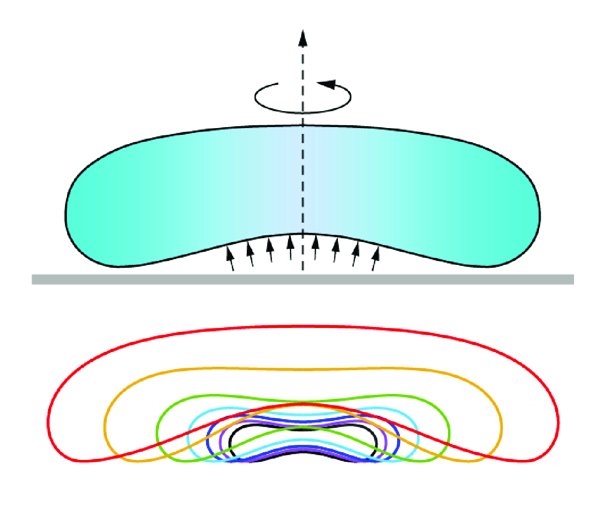
rad s–1 (300 r.p.m.). The surfaces of the drop are marked in colours to indicate that two distinct regions are modelled differently, as described in previous studies (Duchemin et al. Reference Duchemin, Lister and Lange2005; Sobac et al. Reference Sobac, Rednikov, Dorbolo and Colinet2014). The upper liquid–air surface corresponds to the outer drop region, while the lower liquid–vapour surface belongs to the vapour layer region. The governing equations for these regions are discussed separately in the following sections.
Schematic of the full theoretical model employed to investigate the shape and stability of rotating Leidenfrost drops. (a) The drop rotates with a uniform angular velocity
 $\omega$
on a planar surface maintained at a substrate temperature of
 ${T}_{{s}}$
. The radius, height and volume of the drop are denoted by
 ${r}_{{d}}$
,
 ${h}_{{d}}$
and
 ${V}_{{d}}$
, respectively. Panel (b
i) illustrates the two distinct regions of the Leidenfrost drop, each governed by different equations. Panels (b
ii) and (b
iii) provide close-up views that detail the parameters and definitions essential for establishing the governing equations.

2.1. Governing equations for the shape of the vapour layer
Figure 2(b ii) illustrates the details of the geometry and variable definitions. The curvature of the surface in the vapour layer region is controlled by a pressure balance between the vapour and the liquid, which can be described by the Young–Laplace equation
 \begin{equation} p_{{V}} +\gamma \left (\kappa _{{m}} +\kappa _{{a}} \right )=p_{{L}} . \end{equation}
Here,
 ${p}_{{V}}$
and
 ${p}_{{L}}$
denote the pressure of the vapour and liquid phases at the two sides of the liquid–vapour interface, respectively. In addition,
 $\kappa _{{m}}$
and
 $\kappa _{{a}}$
represent the meridional curvature and azimuthal curvature of the liquid–vapour interface. Our model is established in curvilinear coordinates, similar to the approach used by van Limbeek et al. (Reference van Limbeek, Sobac, Rednikov, Colinet and Snoeijer2019), which is a curvilinear coordinates adaptation of the model proposed by Sobac et al. (Reference Sobac, Rednikov, Dorbolo and Colinet2014). We define the arclength of the profile of the drop in the r–z polar coordinate as s, which starts at point o, located at the centre of the drop on the lower liquid–vapour interface. Thus, we have s = 0 at point o. Along the drop profile, as the arclength increases by ds, each variable in (2.1) will also experience a finite change, and the corresponding differential form of (2.1) is expressed as
 \begin{equation} \textrm { d}p_{{V}} +\gamma \left (\textrm{d}\kappa _{{m}} +\textrm { d}\kappa _{{a}} \right )=\textrm { d}p_{{L}} . \end{equation}
At any point on the liquid–vapour interface, the angle between the tangent line at that point and the horizontal line is denoted as
 $\varphi$
. Consequently,
 $\kappa _{{m}}$
and
 $\kappa _{{a}}$
can be expressed as follows (Struik Reference Struik2012; Bostwick & Steen Reference Bostwick and Steen2015):
 \begin{equation} \kappa _{{m}} =\frac {\textrm { d}\varphi }{\textrm { d}s} ,\quad \kappa _{{a}} =\frac {\sin \varphi }{r} . \end{equation}
Additionally, we have the following geometrical relations:
 \begin{equation} \frac {\textrm { d}z}{\textrm { d}s} =\sin \varphi ,\quad \frac {\textrm { d}r}{\textrm { d}s} =\cos \varphi . \end{equation}
The differential of pressure within the liquid near the liquid–vapour interface can be written as
 \begin{equation} \textrm { d}p_{{L}} =-\rho _{{L}} g\textrm { d}z+\rho _{{L}} \omega ^{2} r\textrm { d}r, \end{equation}
where the first term on the right-hand side of (2.5) represents the effect of gravitational force, while the second term arises from the centrifugal force. Combining (2.2) to (2.5) results in
 \begin{equation} \frac {\textrm { d}p_{{V}} }{\textrm { d}s} +\gamma \left [\frac {\textrm { d}\kappa _{{m}} }{\textrm { d}s} +\frac {\cos \varphi }{r} \left (\kappa _{{m}} -\kappa _{{a}} \right )\right ]=-\rho _{{L}} g\sin \varphi +\rho _{{L}} \omega ^{2} r\cos \varphi . \end{equation}
To derive the pressure distribution within the vapour layer, we apply the lubrication approximation, which assumes that both the thickness of the vapour layer and its slope are sufficiently small (Sobac et al. Reference Sobac, Rednikov, Dorbolo and Colinet2014). The pressure gradient within the vapour layer drives an axisymmetric Stokes flow, resulting in a volumetric flux denoted as Q (Duchemin et al. Reference Duchemin, Lister and Lange2005; Sobac et al. Reference Sobac, Rednikov, Dorbolo and Colinet2014),
 \begin{equation} Q=-\frac {z^{3} }{12\mu _{{V}} } \frac {\textrm { d}p_{{V}} }{\textrm { d}r} , \end{equation}
where
 $\mu _{{V}}$
denotes the dynamic viscosity of the vapour. Mass conservation requires that the increased mass flux must be balanced by the evaporation of liquid, leading to
 \begin{equation} \rm {d}\left (2\pi rQ\right )=2\pi rc\textrm { d}r. \end{equation}
Here, c denotes the local evaporation flux, which can be calculated by equating the heat flux of evaporation with the heat conduction through the vapour layer
 \begin{equation} c=\frac {\lambda _{{V}} \Delta T}{\rho _{{V}} Lz} , \end{equation}
where
 $\lambda _{{V}}$
and L denote the thermal conductivity of vapour and the latent heat of evaporation, respectively. Here,
 $\varDelta$
T denotes the superheat, defined as
 $\varDelta$
T =
 ${T}_{{s}}$
–
 ${T}_{{b}}$
, with
 ${T}_{{b}}$
representing the boiling point of the liquid. By substituting (2.7) and (2.9) into (2.8) and considering (2.4), we can derive the differential equation governing the pressure in the vapour layer
 \begin{equation} -\frac {z}{12r\cos \varphi } \frac {\textrm { d}}{\textrm { d}s} \left (\frac {rz^{3} }{\cos \varphi } \frac {\textrm { d}p_{{V}} }{\textrm { d}s} \right )=\frac {\lambda _{{V}} \mu _{{V}} \Delta T}{\rho _{{V}} L} . \end{equation}
To obtain a concise form of differential equations, we introduce a new variable
 $\beta$
,
 \begin{equation} \beta =\frac {rz^{3} }{\cos \varphi } \frac {\textrm { d}p_{{V}} }{\textrm { d}s} . \end{equation}
Subsequently, (2.6) and (2.10) can be, respectively, rewritten as follows:
 \begin{align}&\qquad\qquad\qquad\qquad \frac {\textrm { d}\beta }{\textrm { d}s} =-\frac {12r\cos \varphi }{z} \frac {\lambda _{{V}} \mu _{{V}} \Delta T}{\rho _{{V}} L} , \end{align}
 \begin{align}& \frac {\textrm { d}\kappa _{{m}} }{\textrm { d}s} =-\frac {\cos \varphi }{r} \left (\kappa _{{m}} -\kappa _{{a}} \right )-\frac {\rho _{{L}} g}{\gamma } \sin \varphi +\frac {\rho _{{L}} \omega ^{2} }{\gamma } r\cos \varphi -\frac {\cos \varphi }{\gamma rz^{3} } \beta . \end{align}
Equations (2.3), (2.4), (2.12) and (2.13) form a system of differential equations that can be used to solve
 $\kappa _{{m}}$
,
 $\kappa _{{a}}$
,
 $\varphi$
,
 $\beta$
, z, r as functions of the variable s. In this work, we solve the equations and analyse the results within a non-dimensionalised framework. The self-consistent non-dimensionalisation rules are provided as follows: for length, curvature, volume and pressure variables, non-dimensionalisations are done using
 ${l}_{{c}}$
, 1/
 ${l}_{{c}}$
,
 ${l}_{{c}}^{3}$
and
 $\gamma$
/
 ${l}_{{c}}$
, respectively. All the dimensionless variables are marked by an asterisk
 $^{*}$
.
After non-dimensionalisation, the system of differential equations can be rewritten as
 \begin{equation} \renewcommand {\arraystretch }{2.5} \left \{ \!\!\begin{array}{l} \displaystyle \kappa _{{m}}^{*} = \frac {\textrm { d}\varphi }{\textrm { d}s^{*}}, \quad \kappa _{{a}}^{*} = \frac {\sin \varphi }{r^{*}}, \quad \frac {\textrm { d}z^{*}}{\textrm { d}s^{*}} = \sin \varphi , \quad \frac {\textrm { d}r^{*}}{\textrm { d}s^{*}} = \cos \varphi , \\ \displaystyle \frac {\textrm { d}\beta ^{*}}{\textrm { d}s^{*}} = -\frac {12 r^{*} \cos \varphi }{z^{*}} Ev, \\ \displaystyle \frac {\textrm { d}\kappa _{{m}}^{*}}{\textrm { d}s^{*}} = -\frac {\cos \varphi }{r^{*}} \left ( \kappa _{{m}}^{*} - \kappa _{{a}}^{*} \right ) - \sin \varphi + r^{*} \cos \varphi Ro - \frac {\cos \varphi }{r^{*} z^{*3}} \beta ^{*}. \end{array} \right . \end{equation}
Here, we introduced two dimensionless numbers,
 $Ev$
and Ro, defined as follows:
 \begin{equation} Ev=\frac {\lambda _{{V}} \mu _{{V}} \Delta T}{\gamma l_{{c}} \rho _{{V}} L} ,\;Ro=\frac {\rho _{{L}} \omega ^{2} l_{{c}}^{3} }{\gamma } =\frac {\omega ^{2} l_{{c}} }{g} . \end{equation}
Here
 $Ev$
represents the evaporation number which has been proposed in previous studies (Sobac et al. Reference Sobac, Rednikov, Dorbolo and Colinet2014). Here Ro represents the dimensionless `rotation number’, reflecting the competition between the centrifugal force and the gravitational force acting on a rotating drop with a characteristic length of the order of
 ${l}_{{c}}$
. This definition differs from the previous research (Langbein Reference Langbein2002), where rotation number is quantified using the drop radius (i.e. Rn =
 $\rho _{{L}} \omega ^{2} {r}^{3}/\gamma$
). These two dimensionless numbers together determine the shape of the vapour layer beneath a drop with a given radius
 ${r}_{{d}}^{*}$
. Before § 5, we choose
 $Ev$
=
 $6.26 \times 10^{-7}$
, corresponding to
 $\gamma$
= 0.059 N m
 $^{-1}$
,
 ${l}_{{c}}$
= 0.025 m,
 $\rho _{{V}} = 0.50\,\rm kg\, m^{-3}$
,
 $\mu _{{V}}$
= 1.63
 $\times$
10
 $^{-5}$
Pa s,
 $\lambda _{{V}}$
= 0.032 W m
 $^{-1}$
K
 $^{-1}$
, L = 2.26
 $\times$
10
 $^{6}$
J kg
 $^{-1}$
and
 $\varDelta$
T = 200 K, which represent the properties of water at
 $100^{\,\circ}$
C. These parameters have been chosen in accordance with previous studies (Biance et al. Reference Biance, Clanet and Quéré2003; Chakraborty et al. Reference Chakraborty, Chubynsky and Sprittles2022).
The initial conditions for the variables are specified as follows. At point o, where s = 0, we have
 \begin{equation} \kappa _{{ m}}^{*} |_{s=0} =\kappa _{{ a}}^{*} |_{s=0} =\kappa _{{o}}^{*} ,\; \;z^{*} |_{s=0} =z_{{o}}^{*} ,\; \; r^{*} |_{s=0} =0,\; \;\varphi |_{s=0} =0,\; \;\beta ^{*} |_{s=0} =0. \end{equation}
Here,
 $\kappa _{{o}}^{*}$
and
 ${z}_{{o}}^{*}$
represent the mean curvature and thickness of the vapour layer at point o, which are varied to obtain the shapes of drops with different volumes.
2.2. Governing equations for the shape of the outer drop
As depicted in figure 2(b
iii), a patching point p separates the vapour layer from the outer drop. This patching point is selected at the position where
 $\tan \varphi = 10$
(see point p in figure 2
b
iii), based on previous studies that have demonstrated its negligible influence on numerical results (Duchemin et al. Reference Duchemin, Lister and Lange2005; Sobac et al. Reference Sobac, Rednikov, Dorbolo and Colinet2014). For the outer drop, the pressure balance is similar to that in the vapour layer region, with the distinction that the pressure of the gas phase is fixed at the atmospheric pressure of
 ${p}_{{A}}$
. Thus, we can derive the system of differential equations for the outer drop by simply setting
 $\beta$
 $^{*}$
= 0 in system of (2.14), yielding
 \begin{equation} \renewcommand {\arraystretch }{2.5} \left \{ \!\!\begin{array}{l} \displaystyle \kappa _{{m}}^{*} = \frac {\textrm { d}\varphi }{\textrm { d}s^{*}}, \quad \kappa _{{a}}^{*} = \frac {\sin \varphi }{r^{*}}, \quad \frac {\textrm { d}z^{*}}{\textrm { d}s^{*}} = \sin \varphi , \quad \frac {\textrm { d}r^{*}}{\textrm { d}s^{*}} = \cos \varphi , \\ \displaystyle \frac {\textrm { d}\kappa _{{m}}^{*}}{\textrm { d}s^{*}} = -\frac {\cos \varphi }{r^{*}} \left ( \kappa _{{m}}^{*} - \kappa _{{a}}^{*} \right ) - \sin \varphi + r^{*} \cos \varphi Ro. \end{array} \right . \end{equation}
The initial conditions in the outer drop region when s =
 ${s}_{{p}}$
with
 ${s}_{{p}}$
being the arclength at point p are defined as follows:
 \begin{equation} \kappa _{{m}}^{*} |_{s=s_{{p}} } =\kappa _{mp}^{*} ,\; \;\kappa _{{a}}^{*} |_{s=s_{{p}} } =\kappa _{ap}^{*} ,\; \;z^{*} |_{s=s_{{p}} } =z_{{p}}^{*} ,\; \;r^{*} |_{s=s_{{p}} } =r_{{p}}^{*} ,\; \;\varphi |_{s=s_{{p}} } =\arctan 10. \end{equation}
Here,
 $\kappa _{{mp}}^{*}$
,
 $\kappa _{{ap}}^{*}$
,
 ${z}_{{p}}^{*}$
and
 ${r}_{{p}}^{*}$
represent the values calculated from the governing equations in the vapour layer region at point p. These initial conditions ensure the continuity of drop profile and pressure at the boundary between the two regions.
Finally, (2.14), (2.17) and the initial conditions (2.16), (2.18) allow us to determine the shape of the drop for given values of
 ${z}_{{o}}^{*}$
and
 $\kappa _{{o}}^{*}$
. We employ the standard finite difference method to solve the system of equations, all the unknown variables can evolve with the increase of s
 $^{*}$
with finite difference of ds
 $^{*}$
at each step of iteration. Here, ds
 $^{*}$
is set to 0.0001 to ensure the accuracy of the drop profile. However, not all combinations of
 ${z}_{{o}}^{*}$
and
 $\kappa _{{o}}^{*}$
yield physically meaningful results. Using a shooting method, we can identify an appropriate
 $\kappa _{{o}}^{*}$
for a given
 ${z}_{{o}}^{*}$
that produces a physically realistic drop profile as discussed in detail in Appendix A. Finally, by varying
 ${z}_{{o}}^{*}$
, we can obtain the shapes of drops with different volumes. Notably, our numerical solutions to the full theoretical model converge to those of Sobac et al. (Reference Sobac, Rednikov, Dorbolo and Colinet2014) as Ro
 $\to$
0. To demonstrate the accuracy of our numerical solutions, in Appendix B, we compare the drop profiles calculated in this full theoretical model with previous work (Chakraborty et al. Reference Chakraborty, Chubynsky and Sprittles2022) which has been proved with an almost perfect agreement with the results of Sobac et al. (Reference Sobac, Rednikov, Dorbolo and Colinet2014).
3. Determination of the critical state for chimney instability
By obtaining the numerical solutions to the full theoretical model, we can explore all drop profiles that satisfy the governing equations. However, only subsets of these shapes correspond to the critical states for chimney instability. In this section, we will focus on identifying these subsets and their characteristics.
The solid curves depicted in figure 3(a) demonstrate the relation between drop volume
 ${V}_{{d}}^{*}$
and radius
 ${r}_{{d}}^{*}$
for two different rotation numbers Ro = 0 and Ro = 0.25. Here, Ro = 0.25 corresponds to an angular velocity of
 $\omega$
= 10
 $\pi$
rad s–1, or equivalently, 5 r.p.s. When the drop radius
 ${r}_{{d}}^{*}$
is small,
 ${V}_{{d}}^{*}$
increases following a scaling law of
 ${V}_{{d}}^{*}$
 $\sim$
 ${r}_{{d}}^{*3}$
as illustrated by the log–log plot in figure 3(b). This indicates that the drop assumes a spherical shape, where surface tension force dominates over gravitational and centrifugal forces. As the radius increases, the scaling law gradually transitions to
 ${V}_{{d}}^{*} \sim {r}_{{d}}^{*2}$
, indicating that the drop takes on a puddle shape when gravitational or centrifugal forces dominate over the surface tension force. In addition to the change in scaling relations between
 ${V}_{{d}}^{*}$
and
 ${r}_{{d}}^{*}$
, the monotonicity of the curve also undergoes changes. In the case without rotation (Ro = 0), a maximum value of
 ${V}_{{d}}^{*}$
is observed, marked by the blue circle in the inset of figure 3(a). The corresponding shape of the drop at this critical point is depicted in figure 3(c), with a radius of
 ${r}_{{d}}^{*}$
= 3.96. Following the curve, another critical point with a maximum drop radius is marked by the green circle, where
 ${r}_{{d}}^{*}$
= 3.99. The curve terminates at the red circle, where the lower liquid–vapour interface of the drop touches its apex at
 ${r}_{{d}}^{*}$
= 3.72. While mathematical solutions of the drop profile can still be obtained beyond this point, the lower liquid–vapour interface would exceed the height of the upper one. However, these solutions are unphysical and should be excluded, as the drop will undergo a topological transformation, forming a chimney at the centre and transitioning into a liquid torus (Quéré Reference Quéré2013). For the case with rotation (Ro = 0.25), only two critical points are observed: one representing the maximum volume and the other indicating the surface touch state, occurring at
 ${r}_{{d}}^{*}$
= 3.08 and
 ${r}_{{d}}^{*}$
= 3.18, respectively.
Analysis of the critical state for chimney instability. (a) The variation of
 ${V}_{{d}}^{*}$
with
 ${r}_{{d}}^{*}$
under two different values of Ro. The insets provide enlarged views of the end sections of the
 ${V}_{{d}}^{*}$
–
 ${r}_{{d}}^{*}$
curves. The red circles correspond to the surface touch states, while the green and blue circles correspond to the maximum volume states. (b) The same
 ${V}_{{d}}^{*}$
–
 ${r}_{{d}}^{*}$
curves presented in a log–log plot, illustrating the scaling relations between
 ${V}_{{d}}^{*}$
and
 ${r}_{{d}}^{*}$
at their lower and upper bounds, respectively. (c) The numerical results of drop profile and radius at the critical points highlighted in figure 3(a).

Critical state for chimney instability under different Ro. (a) Illustration of critical points for chimney instability as Ro increases in the
 ${V}_{{d}}^{*}$
–
 ${r}_{{d}}^{*}$
diagram. The inset illustrates the scaling relation between
 ${V}_{{c}}^{*}$
and
 ${r}_{{c}}^{*}$
in a log–log plot. Panel (a
ii) shows the drop profile at a fixed Ro = 0.25, with increasing
 ${V}_{{d}}^{*}$
(values indicated). The profile corresponding to the critical state is highlighted in blue. (b) Illustration of critical points for chimney instability as
 ${V}_{{d}}^{*}$
increases in the
 ${r}_{{d}}^{*}$
–Ro diagram. The inset illustrates the relation between
 ${r}_{{c}}^{*}$
and Ro in a log–log plot. Panel (b
ii) shows the drop profile at a fixed
 ${V}_{{d}}^{*}$
= 31.21 with increasing Ro (values indicated). The profile at the critical state is highlighted in blue. (c) Numerical solutions of drop profiles at the critical state with different values of Ro.

For all critical points, we select the point with the maximum drop volume as the criterion for chimney instability. In a scenario where the drop volume increases continuously by adding liquid, when the volume exceeds the maximum volume indicated on the
 ${V}_{{d}}^{*}$
–
 ${r}_{{d}}^{*}$
curve, there are no solutions that satisfy the governing equations for a Leidenfrost drop. Thus, the drop will experience dynamic evolution and enter a state of chimney instability. By employing this criterion, the critical radius for the chimney instability of a non-rotating drop, as calculated by our numerical solution, is
 ${r}_{{c}}^{*}$
= 3.96. This value agrees very well with previous experimental (
 ${r}_{{c}}^{*}$
= 4.0) (Biance et al. Reference Biance, Clanet and Quéré2003), theoretical (
 ${r}_{{c}}^{*}$
= 3.95) (Snoeijer et al. Reference Snoeijer, Brunet and Eggers2009) and simulation results (
 ${r}_{{c}}^{*}$
= 3.97) (Chakraborty et al. Reference Chakraborty, Chubynsky and Sprittles2022). Furthermore, this maximum volume criterion has also been adopted in other studies to determine the critical state for the instability of liquid annuli (Lv & Hardt Reference Lv and Hardt2021) and pendant drops (Zhang & Zhou Reference Zhang and Zhou2023).
In figure 4(a), we present the
 ${V}_{{d}}^{*}$
–
 ${r}_{{d}}^{*}$
curves and highlight the critical state for varying Ro from 0 to 9.05, corresponding to angular velocity from 0 rad s–1 to 60
 $\pi$
rad s–1 for boiling water with g = 9.81 m s–
 $^{2}$
. The results indicate that an increase in Ro leads to chimney instability occurring at smaller drop sizes, both in terms of volume and radius. The critical drop volume and radius for chimney instability are denoted as
 ${V}_{{c}}^{*}$
and
 ${r}_{{c}}^{*}$
, respectively. Interestingly, although
 ${V}_{{d}}^{*}$
and
 ${r}_{{d}}^{*}$
follow different scaling relations with the exponent changing from 3 to 2 as discussed in the above, the scaling relation between
 ${V}_{{c}}^{*}$
and
 ${r}_{{c}}^{*}$
follows
 ${V}_{{c}}^{*}$
= 1.37
 ${r}_{{c}}^{*2.86}$
as Ro varies, which is close to
 ${V}_{{c}}^{*}$
 $\sim {r}_{{c}}^{*3}$
as marked by the triangle in the log–log plot. This scaling relation will be further elaborated in § 4. In figure 4(a
ii), we present drop profiles at a fixed Ro = 0.25, with
 ${V}_{{d}}^{*}$
increasing to observe how the drop shape evolves before the onset of chimney instability. Initially, as
 ${V}_{{d}}^{*}$
increases from 2.97 to 15.77, the drop grows in both height and radius, exhibiting a puddle-like shape. However, when
 ${V}_{{d}}^{*}$
increases further from 15.77 to 31.21 (the critical state), the drop radius continues to expand while its height decreases, and the top surface becomes concave, indicating elongation due to the centrifugal force. In figure 4(b), we reorganise the data from figure 4(a) to illustrate the relation between
 ${r}_{{d}}^{*}$
and Ro while keeping
 ${V}_{{d}}^{*}$
fixed for each curve. Along the direction indicated by the arrow,
 ${V}_{{d}}^{*}$
varies from 2 to 68 in increments of 2. For each curve,
 ${r}_{{d}}^{*}$
initially increases with Ro starting from Ro = 0. However, each curve reaches a critical point, identified by the maximum value of Ro, beyond which no solutions exist. Going beyond these critical points marked by blue circles, the curves extend to terminal points defined by the surface-touch state. These critical points correspond precisely to those determined by the maximum volume criterion in figure 4(a). Additionally, the curves in figure 4(b) reveal that drops with larger volumes are more sensitive to rotation, with chimney instability occurring at smaller Ro. The inset presents these critical points in log–log coordinates, exhibiting two distinct trends at small and large Ro, which will be discussed in § 4. Similarly, in figure 4(b
ii), we present drop profiles at a fixed
 ${V}_{{d}}^{*}$
= 31.21 while increasing Ro. Without rotation (Ro = 0), the drop already exhibits a puddle-like shape. As Ro increases, the drop elongates further, with its radius increasing and height decreasing, until the chimney instability occurs at Ro = 0.25. Figures 4(a) and 4(b) demonstrate that the same drop profile at the critical state for chimney instability applies not only to the instability reached by increasing drop volume at a constant angular velocity but also to the instability reached by increasing angular velocity at a constant drop volume.
We further present the drop profiles at the critical states with different values of Ro, as illustrated and discussed in figure 4(c). At small Ro, the upper surface of the drop is nearly flat compared with its lower counterpart. However, as Ro increases, the upper surface curves inwards, similar to its lower counterpart, due to the centrifugal force stretching the drop along the radial direction. Despite these differences, all drops maintain a similar puddle shape, with both their radius and height decreasing with increasing Ro. This similarity in puddle shape will be explained by our simplified theoretical model in § 4. Additionally, it is worth noting that in our full theoretical model, the internal flow of the drop is assumed to move solely in the azimuthal direction. However, in reality, the internal flow of a Leidenfrost drop exhibits axisymmetric motion (Bouillant et al. Reference Bouillant, Mouterde, Bourrianne, Lagarde, Clanet and Quéré2018a ; Chakraborty et al. Reference Chakraborty, Chubynsky and Sprittles2022). Previous studies have shown that the influence of such motion on the shape and stability of real non-rotating Leidenfrost drops is negligible, possibly due to the rolling motion induced by symmetry breaking (Yim et al. Reference Yim, Bouillant, Quere and Gallaire2022), which weakens the azimuthally averaged axisymmetric flow (Chakraborty et al. Reference Chakraborty, Chubynsky and Sprittles2022). In Appendix C, we demonstrate that this effect is even less significant for rotating Leidenfrost drops. Therefore, the impact of internal liquid motion on the onset of chimney instability is neglected in this study.
4. Simplified theoretical model
In this section, we will explore how the geometrical parameters at the critical state change with Ro. A simplified theoretical model is developed to provide theoretical explanations and approximate solutions of the scaling relations presented here, as well as for the scaling relation of
 ${V}_{{c}}^{*} \sim {r}_{{c}}^{*3}$
established in the previous section.
4.1. Phase diagrams and scaling relations of chimney instability
The phase diagram effectively illustrates how the critical conditions for instability vary with Ro, as presented in figure 5(a–c). In all these figures,
 $Ev$
is maintained constant at 6.26
 $\times$
10
 $^{-7}$
, while Ro is varied. As discussed in figure 4(c), for each value of Ro, a unique critical drop profile can be determined, with each profile corresponding to a specific set of critical parameters (
 ${r}_{{c}}^{*}, {h}_{{c}}^{*}$
and
 ${V}_{{c}}^{*}$
). These critical parameters form the blue critical points in figure 5(a–c). For any given Ro, if the values of
 ${r}_{{d}}^{*}$
,
 ${h}_{{d}}^{*}$
or
 ${V}_{{d}}^{*}$
for a drop fall within the stable (green) region of the phase diagram, the drop remains stable; otherwise, it becomes unstable, characterised by bubbles formation and popping. It is evident that, in the linear coordinate system,
 ${r}_{{c}}^{*}$
,
 ${h}_{{c}}^{*}$
and
 ${V}_{{c}}^{*}$
all decrease rapidly as Ro increases from zero, but exhibit a much smoother rate of decrease at higher values of Ro.
In figure 5(d-f), we present the critical points for chimney instability using log–log plots to identify the scaling relations. The trends observed in these curves suggest that the scaling relations behave differently for Ro below and above a transition Ro number,
 $\textit{Ro}_{t}$
, which is chosen as
 $\textit{Ro}_{t} = 0.15 $
, as marked by the black solid line in figure 5(d-f). The rationale for choosing
 $\textit{Ro}_{t} = 0.15$
will be elaborated in the next section. When Ro
 $\ll$
 $\textit{Ro}_{t}$
, the critical parameters are minimally affected by Ro, with values similar to those of non-rotating Leidenfrost drops, showing good agreement with chimney instability criteria established in previous studies (Biance et al. Reference Biance, Clanet and Quéré2003; Snoeijer et al. Reference Snoeijer, Brunet and Eggers2009; Chakraborty et al. Reference Chakraborty, Chubynsky and Sprittles2022). The results indicate scaling relations of
 ${r}_{{c}}^{*}$
= 3.96
 $\sim$
Ro
 ${}^{0}$
,
 ${h}_{{c}}^{*}$
= 2.12
 $\sim$
Ro
 ${}^{0}$
and
 ${V}_{{c}}^{*}$
= 71.00
 $\sim$
Ro
 ${}^{0}$
for Ro
 $\ll$
 $\textit{Ro}_{t}$
. These values are obtained from the drop profile at critical state with Ro = 0. However, when Ro
 $\gg$
 $\textit{Ro}_{t}$
, distinct scaling relations emerge. By fitting the data with Ro
 $\gg$
 $\textit{Ro}_{t}$
, the critical drop radius, height and volume follow the relations of
 ${r}_{{c}}^{*}$
= 2.37Ro
 ${}^{-0.33}$
,
 ${h}_{{c}}^{*}$
= 0.95Ro
 ${}^{-0.28}$
,
 ${V}_{{c}}^{*}$
= 15.98Ro
 ${}^{-0.97}$
, respectively. The fitting is conducted using a linear regression of data points with Ro
 $\gt$
20
 $\textit{Ro}_{t}$
. These relations are close to the scaling relations of
 ${r}_{{c}}^{*}$
 $\sim$
Ro
 ${}^{-1/3}$
,
 ${h}_{{c}}^{*}$
 $\sim$
Ro
 ${}^{-1/3}$
and
 ${V}_{{c}}^{*}$
 $\sim$
Ro
 ${}^{-1}$
as shown by the triangles marked near the critical points. According to the definition of Ro, we categorise these two regions with different scaling relations as ‘gravity-dominated’ and ‘rotation-dominated’, which are distinguished by background colours in figure 5(d–f).
Phase diagram and scaling relations of chimney instability. (a),(b),(c) Phase diagrams depicting the parameter space for stable and unstable drops under varying Ro, with
 ${r}_{{d}}^{*}$
,
 ${h}_{{d}}^{*}$
and
 ${V}_{{d}}^{*}$
as the variables. The inset in (c) provides a zoomed-in view for Ro ranging from 0 to 3. (d), (e), (f) Scaling relations between the critical parameters
 ${r}_{{c}}^{*}$
,
 ${h}_{{c}}^{*}$
,
 ${V}_{{c}}^{*}$
and Ro. The background colour indicates the influence of rotation relative to gravity on chimney instability. Solid black lines indicate the transitional Ro, denoted as Ro
 ${}_{{t}}$
= 0.15.

Illustration of the geometrical simplifications used in pressure balance and perturbation analyses. (a) The puddle drop is modelled as a cylindrical shape with a height of
 ${h}_{{c}}$
and a radius of
 ${r}_{{c}}$
. The pressures
 ${p}_{{A}}$
,
 ${p}_{{La}}$
and
 ${p}_{{S}}$
represent the atmospheric pressure, average liquid pressure and Laplace pressure, respectively. (b) For a gravity-dominated instability, a sinusoidal perturbation
 $\delta$
h(r) is introduced at the bottom of the drop, resulting in a radial expansion of the drop by
 $\delta {r}_{{c}}$
. For a rotation-dominated chimney instability, perturbations
 $\delta$
h(r) occur at both the top and the bottom of the drop, leading to a radial expansion of
 $\delta {r}_{{c}}$
. The pressures
 ${p}_{{V}}$
,
 ${p}_{{L1}}$
,
 ${p}_{{L2}}$
,
 ${p}_{{S1}}$
and
 ${p}_{{S2}}$
represent the atmospheric pressure, liquid pressures at the centre and rim of the bottom surface, Laplace pressures at the centre and rim of the bottom surface, respectively.

4.2. Pressure balance analyses
Here, we delve into elucidating the distinct scaling relations discussed in the above. Firstly, we simplify the drop configuration based on its primary shape characteristics to facilitate pressure balance analyses. As demonstrated in figure 4(c), for all values of Ro, the shapes of the drops at critical states resemble puddles, with their radial length scale significantly larger than their height scale. Consequently, the profile of the drop can be simplified into a cylindrical shape, as shown in figure 6(a), featuring flat surfaces on the top and bottom, and a curved surface at the rim.
The distribution of liquid pressure along the zaxis at the rim is denoted as
 ${p}_{{L}}$
and is given by
 ${p}_{{L}} = {p}_{{A}} + (1/2) \rho \omega {}^{2}{r}_{{c}} {}^{2} + \rho g({h}_{{c}} - {z})$
, where
 ${p}_{{A}}$
represents atmospheric pressure, and we assume that the drop rim has a uniform radius
 ${r}_{{c}}$
. The second term in
 ${p}_{{L}}$
represents the pressure due to centrifugal force, while the third term accounts for hydrostatic pressure, which decreases with z. Consequently, we can derive the average pressure
 ${p}_{{L}}$
 ${}_{{a}}$
exerted on the drop rim as follows:
 \begin{equation} p_{{ La}} = \frac {1}{h_{{ c}}} \int _{0}^{h_{{ c}}} p_{{ L}} \, \textrm { d}z = p_{{ A}} + \frac {1}{2} \rho \omega ^{2} r_{{ c}}^{2} + \frac {1}{2} \rho g h_{{ c}}. \end{equation}
On the other hand,
 ${p}_{{La}}$
must be balanced by two other pressure components at the drop rim. The first component is the atmospheric pressure at the rim, also denoted as
 ${p}_{{A}}$
, and the second is the average Laplace pressure generated by the surface tension at the rim, which can be approximated by
 ${p}_{{S}}$
=
 $\gamma [2/{h}_{{c}}+\pi /(4{r}_{{c}})]$
(Park & Homsy Reference Park and Homsy1984; Dangla, Kayi & Baroud Reference Dangla, Kayi and Baroud2013; Lv et al. Reference Lv, Zhang, Shi and Hao2020). The term in the square brackets corresponds to the principal curvatures of the drop rim (Lv et al. Reference Lv, Zhang, Shi and Hao2020). Thus, we have
 ${p}_{{La}}$
=
 ${p}_{{A}} +\gamma [2/{h}_{{c}}+\pi /(4 {r}_{{c}})]$
. Therefore, we obtain the pressure balance at the rim as
 \begin{equation} \frac {1}{2} \rho \omega ^{2} r_{{c}}^{2} + \frac {1}{2} \rho g h_{{c}} = \gamma \left ( \frac {2}{h_{{c}}} + \frac {\pi }{4 r_{{c}}} \right ). \end{equation}
Variations of relative pressures with Ro. (a) The ratio of
 ${p}_{{R}}$
/
 ${p}_{{G}}$
as a function of Ro. The dashed line indicates the condition where
 ${p}_{{R}} / {p}_{{G}}$
= 1. (b) Variation of Bo with Ro. The red circles represent Bo defined by
 ${p}_{{G}} / {p}_{{S}}$
, (4.4), while the blue circles represent Bo defined by
 ${p}_{{R}} / {p}_{{S}}$
, (4.5). The black curve is the sum of these two types of Bond numbers (
 ${p}_{{G}} / {p}_{{S}} + {p}_{{R}} / {p}_{{S}}$
). The solid lines in both panels correspond to
 ${Ro}_{{t}}$
= 0.15.

Here, we denote the first and second terms on the left-hand side of (4.2) as the rotation-induced pressure
 ${p}_{{R}} = 1/2\rho \omega {}^{2} {r}_{{c}} {}^{2}$
and the gravity-induced pressure
 ${p}_{{G}}$
= 1/2
 $\rho$
gh
 $_{{c}}$
, respectively. Equation (4.2) indicates that
 ${p}_{{R}}$
and
 ${p}_{{G}}$
jointly determine the geometry of drop at the rim, with the ratio between them dictating whether rotation or gravity plays a dominant role. The expression for
 ${p}_{{R}}$
/
 ${p}_{{G}}$
is
 \begin{equation} \frac {p_{{R}}}{p_{{G}}} = \frac {\dfrac {1}{2} \rho \omega ^{2} r_{{c}}^{2}}{\dfrac {1}{2} \rho g h_{{c}}} = \frac {r_{{c}}^{*2}}{h_{{c}}^{*}} \, \textit {Ro}. \end{equation}
Although, according to its definition in (2.15), Ro represents the competition between the centrifugal and gravitational force with a characteristic length scale of
 ${l}_{{c}}$
, it does not precisely reflect the competition between
 ${p}_{{R}}$
and
 ${p}_{{G}}$
at the drop rim. Instead, a correction factor of
 ${r}_{{c}}^{*2}$
/
 ${h}_{{c}}^{*}$
exists between Ro and
 ${p}_{{R}}$
/
 ${p}_{{G}}$
. By substituting
 ${h}_{{c}}^{*}$
and
 ${r}_{{c}}^{*}$
obtained from the numerical results into (4.3), the variation of
 ${p}_{{R}}$
/
 ${p}_{{G}}$
with Ro is provided in figure 7(a), where we observe a positive correlation. When
 ${p}_{{R}}$
=
 ${p}_{{G}}$
, which represents the condition where the roles of rotation and gravity are equivalent in determining the drop shape, the value of Ro is 0.15. This analysis reveals the physical mechanism behind choosing
 ${Ro}_{{t}}$
= 0.15. As Ro increases beyond
 ${Ro}_{{t}}$
, the rotation-induced pressure gradually becomes dominant. Therefore,
 ${Ro}_{{t}}$
serves to calibrate the transition between the gravity-dominated and rotation-dominated scaling regions in figure 5. The Bond number Bo is defined as the ratio of gravitational to capillary forces (Langbein Reference Langbein2002), and it determines the shape of the capillary surface under gravity, such as in sessile (Yariv & Schnitzer Reference Yariv and Schnitzer2023) and pendant drops (Zhang & Zhou Reference Zhang and Zhou2023). Analogous to the traditional definition of Bo, in our context of rotating Leidenfrost drops, the concept of gravitational force is extended to include centrifugal force. Therefore, Bo can be defined in two ways,
 \begin{equation} \frac {p_{{G}}}{p_{{S}}} = \frac {\dfrac {1}{2} \rho g h_{{c}}}{\gamma \left ( \dfrac {2}{h_{{c}}} + \dfrac {\pi }{4 r_{{c}}} \right )} = \frac {h_{{c}}^{*}}{\dfrac {4}{h_{{c}}^{*}} + \dfrac {\pi }{2 r_{{c}}^{*}}}, \end{equation}
 \begin{equation} \frac {p_{{R}}}{p_{{S}}} = \frac {\dfrac {1}{2} \rho \omega ^{2} r_{{c}}^{2}}{\gamma \left ( \dfrac {2}{h_{{c}}} + \dfrac {\pi }{4 r_{{c}}} \right )} = \dfrac {r_{{c}}^{*2} \, \textit {Ro}}{\dfrac {4}{h_{{c}}^{*}} + \dfrac {\pi }{2 r_{{c}}^{*}}}, \end{equation}
where
 ${p}_{{G}}$
represents the pressure due to gravity,
 ${p}_{{R}}$
the pressure due to rotation and
 ${p}_{{S}}$
the capillary pressure. In figure 7(b), by substituting the
 ${h}_{{c}}^{*}$
and
 ${r}_{{c}}^{*}$
obtained from the numerical results into (4.4) and (4.5), we illustrate how these two types of Bo vary with Ro. The two sets of data points intersect at Ro =
 ${Ro}_{{t}}$
= 0.15. In the gravity-dominated regime,
 ${p}_{{G}}$
/
 ${p}_{{S}}$
dominates, while in the rotation-dominated regime,
 ${p}_{{R}}$
/
 ${p}_{{S}}$
takes over. The sum (
 ${p}_{{G}}$
/
 ${p}_{{S}}$
+
 ${p}_{{R}}$
/
 ${p}_{{S}}$
) of the two Bonds number remains nearly constant, around 1. This result suggests that, whether gravity or rotation is dominant, at the critical state for chimney instability, the total value of Bo remains similar. This finding, to some extent, explains the shape similarity observed in figure 4(c), where drops at the critical states all exhibit a puddle shape. It should also be clarified that since
 ${p}_{{G}}$
/
 ${p}_{{S}}$
+
 ${p}_{{R}}$
/
 ${p}_{{S}}$
= 1 is a straightforward consequence of (4.2), this result also serves as a validation of the pressure balance in the simplified theoretical model.
4.3. Pressure perturbation analyses
Second, we proceed with an analysis of the critical conditions for chimney instability. In dimensionless form, (4.2) can be written as
 \begin{equation} \frac {r_{{c}}^{*2} \, \textit {Ro}}{2} + \frac {h_{{c}}^{*}}{2} = \frac {2}{h_{{c}}^{*}} + \frac {\pi }{4 r_{{c}}^{*}}. \end{equation}
For puddles, considering 2
 ${r}_{{c}}^{*}$
 $\gg$
 ${h}_{{c}}^{*}$
, (4.6) simplifies to
 \begin{equation} \frac {r_{{c}}^{*2} \, \textit {Ro}}{2} + \frac {h_{{c}}^{*}}{2} = \frac {2}{h_{{c}}^{*}}. \end{equation}
In the gravity-dominated regime where Ro
 $\ll$
 ${Ro}_{{t}}$
, (4.7) yields
 \begin{equation} h_{{c}}^{*} = 2 \sim \textit {Ro}^{0}, \end{equation}
which represents the maximum height of liquid puddles (de Gennes et al. Reference de Gennes, Brochard-Wyart and Quere2004) and is independent of Ro. However, the value obtained is slightly smaller than the numerical solution of
 ${h}_{{c}}^{*}$
= 2.12 from the full theoretical model. This discrepancy can be attributed to the fact that, in our simplified theoretical model, the thickness of the vapour layer is neglected, leading to a certain underestimation of the drop height. In the rotation-dominated regime where Ro
 $\gg$
 ${Ro}_{{t}}$
and regarding 2
 ${r}_{{c}}^{*}$
 $\gg$
 ${h}_{{c}}^{*}$
, (4.7) simplifies to
 \begin{equation} r_{{c}}^{*2} h_{{c}}^{*} \, \textit {Ro} = 4. \end{equation}
The term
 ${h}_{{c}}^{*}$
/2 in (4.7) is omitted to obtain (4.9) because it decreases and approaches 0 as Ro
 $\gg$
 ${Ro}_{{t}}$
. We illustrate the variation of
 ${r}_{{c}}^{*2}{h}_{{c}}^{*}$
Ro with Ro in figure 8(a) based on the numerical results. The plot clearly shows that the growth rate of
 ${r}_{{c}}^{*2}{h}_{{c}}^{*}$
Ro gradually decreases as Ro increases, although a finite slope persists. By averaging the data points for Ro
 $\gt$
20
 ${Ro}_{{t}}$
, we obtain a mean value of
 ${r}_{{c}}^{*2}{h}_{{c}}^{*}$
Ro = 6.61, which exceeds the approximate solution in (4.9). Moreover, the finite slope can be partially explained by the omission of the term
 ${h}_{{c}}^{*}$
/2 in (4.7). If not omitted, this term would contribute an additional term of –
 ${h}_{{c}}^{*2}$
to the right-hand side of (4.9). This term can be significant for values of Ro that are not substantially larger than
 ${Ro}_{{t}}$
. As shown in figure 5(e), for Ro = 1, 10, 100, the values of –
 ${h}_{{c}}^{*2}$
are –0.91, –0.25 and –0.07, respectively, with variations that are relatively prominent compared with 4.0.
(a) Variation of
 ${r}_{{c}}^{*2}{h}_{{c}}^{*}$
Ro and
 ${r}_{{c}}^{*4}{h}_{{c}}^{*-1}$
Ro as functions of Ro. The circles represent the numerical results, while the dashed lines indicate the approximate solutions for Ro
 $\gg$
 ${Ro}_{{t}}$
. The red and blue dashed lines are the approximate solutions obtained from (4.9) and (4.23), respectively. (b) Variation of
 ${r}_{{c}}^{*}$
with Ro. The blue circles represent the numerical results, while the solid and dashed red curves indicate the implicit approximate solutions for Ro
 $\gt$
 ${Ro}_{{t}}$
, (4.29), and Ro
 $\lt$
 ${Ro}_{{t}}$
, (4.30), respectively. The solid lines in both panels correspond to
 ${Ro}_{{t}}$
= 0.15.

Then, shape and pressure perturbation are added to the drop, which are discussed separately in gravity-dominated and the rotation-dominated regimes. In the gravity-dominated regime where Ro
 $\ll$
 ${Ro}_{{t}}$
, as observed in figure 4(c), the shape change mainly occurs at the lower surface. Therefore, for our analyses in this regime, we focus only on perturbations introduced at the lower surface, as depicted in figure 6(b). We assume the perturbation of the lower surface takes on a sinusoidal form (Biance et al. Reference Biance, Clanet and Quéré2003)
 \begin{equation} \delta h\left (r\right ) = \varepsilon \left (1 + \cos \frac {\pi r}{r_{{c}}}\right ). \end{equation}
Here,
 $\varepsilon$
is a minimum representing the magnitude of the perturbation, with
 $\varepsilon$
 $\ll$
 ${h}_{{c}}$
. The height of the drop is assumed to remain constant. The volume of vapour underneath the perturbed surface is given by
 \begin{equation} \delta V = \int _{0}^{r_{{c}}} 2\pi r \, \delta h \, {\rm d}r = \int _{0}^{r_{{c}}} 2\pi r \varepsilon \left (1 + \cos \frac {\pi r}{r_{{c}}}\right ) \, {\rm d}r = \left (\pi - \frac {4}{\pi }\right ) \varepsilon r_{{c}}^{2}. \end{equation}
According to the mass conservation of liquid, the drop radius must increase by
 $\delta {r}_{{c}}$
to compensate for
 $\delta$
V, leading to 2
 $\pi {r}_{{c}}{h}_{{c}}\delta {r}_{{c}}$
=
 $\delta$
V. Consequently, we obtain
 \begin{equation} \delta r_{{c}} = \left (\frac {1}{2} - \frac {2}{\pi ^{2}}\right ) \frac {r_{{c}}}{h_{{c}}} \varepsilon . \end{equation}
Meanwhile, the perturbation in geometry will also induce a perturbation in the pressure distribution. As denoted in figure 6(b),
 ${p}_{{L1}}$
represents the pressure of the liquid at the centre of the drop bottom. This pressure must be balanced by the vapour pressure
 ${p}_{{V}}$
and the Laplace pressure at the centre of the bottom surface denoted as
 ${p}_{{S1}}$
, leading to
 ${p}_{{L1}}$
–
 ${p}_{{V}}$
–
 ${p}_{{S1}}$
= 0. In this perturbation analysis, the pressure of the vapour is assumed to be uniform throughout the space (Biance et al. Reference Biance, Clanet and Quéré2003). The perturbation of the bottom surface introduces a change in the pressure balance represented as
 $\delta$
(
 ${p}_{{L1}}$
–
 ${p}_{{V}}$
–
 ${p}_{{S1}}$
). If
 $\delta$
(
 ${p}_{{L1}}$
–
 ${p}_{{V}}$
–
 ${p}_{{S1}}$
) increases with
 $\varepsilon$
, i.e.
 $\delta$
(
 ${p}_{{L1}}$
–
 ${p}_{{V}}$
–
 ${p}_{{S1}}$
)
 $\gt$
0, the perturbation of the bottom surface will be restrained, indicating a stable state. Conversely, if
 $\delta$
(
 ${p}_{{L1}}$
–
 ${p}_{{V}}$
–
 ${p}_{{S1}}$
)
 $\lt$
0, the initial perturbations will progress, causing the liquid to flow from the centre to the rim of the drop, eventually resulting in chimney instability. Thus, the stability criterion can be expressed as
 \begin{equation} \delta p_{{L1}} - \delta p_{{V}} - \delta p_{{S1}} = 0. \end{equation}
Here, we select the liquid pressure at the rim of the drop bottom
 ${p}_{{L2}}$
as the reference pressure. Given that
 ${p}_{{L2}} = {p}_{{A}} +\rho gh_{{c}}$
remains unchanged under perturbation, we have
 $\delta {p}_{{L2}}$
= 0. Since
 ${p}_{{L1}} = {p}_{{L2}} - \rho gh_{{V}}$
with
 ${h}_{{V}}$
= 2
 $\varepsilon$
denoting the height of the vapour layer at the bottom centre, we can obtain
 \begin{equation} \delta p_{{L1}} = \delta \left (p_{{L2}} - \rho g h_{{V}}\right ) = -\rho g \delta h_{{V}} = -2 \rho g \varepsilon . \end{equation}
Here,
 $\delta h_{{V}}$
= 2
 $\varepsilon$
, because the solid–liquid interface is flat (i.e.
 ${h}_{{V}}$
= 0) in the absence of perturbation. The pressure balance at the rim of the drop bottom yields
 ${p}_{{V}}$
=
 ${p}_{{L2}}$
–
 ${p}_{{S2}}$
. The perturbation of the curvature at the rim of the bottom surface can be calculated using the curvature of the curve
 $\delta$
h(r) (Biance et al. Reference Biance, Clanet and Quéré2003), yielding
 $\delta \kappa _{{S2}} = \pi^{2} \varepsilon$
/
 ${r}_{{c}}^{2}$
. Thus,
 $\delta {p}_{{V}}$
can be deduced as
 \begin{equation} \delta p_{{V}} = \delta \left (p_{{L2}} - p_{{S2}}\right ) = - \delta \left (\gamma \kappa _{{S2}}\right ) = -\gamma \delta \kappa _{{S2}} = -\gamma \pi ^2 \frac {\varepsilon }{r_{{c}}^{2}}. \end{equation}
Similarly, the perturbation of the Laplace pressure at the centre of the drop bottom is given by (Biance et al. Reference Biance, Clanet and Quéré2003)
 \begin{equation} \delta p_{{S1}} = \delta \left (\gamma \kappa _{{S1}}\right ) = \gamma \delta \kappa _{{S1}} = -2\gamma \pi ^2 \frac {\varepsilon }{r_{{c}}^{2}}. \end{equation}
Here,
 $\kappa _{{S1}}$
and
 $\kappa _{{S2}}$
represent the total curvatures of the liquid–vapour interface at the bottom centre and the bottom rim, respectively. Their values are defined as negative and positive, indicating downward and upward curves when viewed from the side of the drop profile, as illustrated in figure 6(b). By substituting (4.14)–(4.16) into (4.13), we can determine the critical radius for chimney instability as
 \begin{equation} r_{{c}}^{*} = \sqrt {\frac {3}{2}} \pi \approx 3.85 \sim \textit {Ro}^{0}, \end{equation}
which is slightly smaller than the numerical result of
 ${r}_{{c}}^{*}$
= 3.96 from the full theoretical model. The stability analysis presented above is based on previous work (Biance et al. Reference Biance, Clanet and Quéré2003), which leads to the same conclusion as that derived in (4.17). Equations (4.8) and (4.17) together indicate that in the gravity-dominated regime where Ro
 $\ll$
 ${Ro}_{{t}}$
, both the drop radius and height approach fixed values that are independent of Ro. This outcome is a natural consequence of the asymptotic case, where the effects of Ro are considered negligible. It is consistent with the scaling relations
 ${r}_{{c}}^{*} {\sim } {Ro}^{0}$
and
 ${h}_{{c}}^{*}{\sim } {Ro}^{0}$
, as supported by the numerical results presented in figures 5(d) and 5(e), respectively. For the simplified cylindrical configuration of the drop, the volume can be approximated as
 ${V}_{{c}}^{*} \approx \pi r_{{c}}^{*2}{h}_{{c}}^{*}$
. Thus, the volume of the drop should also follow the relation
 \begin{equation} V_{{c}}^{*} = 3\pi ^3 \approx 93.02 \sim \textit {Ro}^{0}, \end{equation}
which is consistent with the scaling relation observed in figure 5( f). However, this approximate result is larger than the numerical result of
 ${V}_{{c}}^{*}$
= 71.0, which is attributed to the simplification of the drop profile, neglecting the volume occupied by the vapour layer at the bottom.
Here, we extend the stability analyses to identify the critical conditions for the rotation-dominated instability. Figure 4(c) demonstrates that in the rotation-dominated regime where Ro
 $\gg$
 ${Ro}_{{t}}$
, both the upper and lower surfaces curve inward into the drop at the critical state. As Ro increases, the changes in the upper and the lower surfaces become indistinguishable. Consequently, perturbations are introduced on both the upper and the lower surface of the drop for rotation-dominated instability, as shown in figure 6(b). The perturbation of the surface remains the same as presented in (4.10). However, since both surfaces are curved, the perturbations in volume and radius are doubled compared with those in the gravity-dominated regime. Thus, we have
 \begin{equation} \delta r_{{c}} = \left (1 - \frac {4}{\pi ^{2}}\right )\frac {r_{{c}}}{h_{{c}}} \varepsilon . \end{equation}
In contrast to the gravity-dominated condition, the expression for
 ${p}_{{L1}}$
is now given by
 ${p}_{{L1}}$
=
 ${p}_{{L2}}$
–
 $\rho gh_{{V}}$
– 1/2
 $\rho \omega ^{2}{r}_{{c}}^{2}$
. The additional term accounts for the pressure arising from the centrifugal force. Thus, the perturbation
 $\delta {p}_{{L1}}$
for the rotating drop is expressed as
 \begin{equation} \begin{aligned} { \delta }p_{{L1}} & = { \delta }\left (p_{{L2}} -\rho gh_{{V}} -\frac {1}{2} \rho \omega ^{2} r_{{c}}^{2} \right ) = -\rho g { \delta }h_{{V}} -\rho \omega ^{2} r_{{c}} { \delta }r_{{c}} \\ & = -2\rho g\varepsilon -\rho \omega ^{2} \left (1-\frac {4}{\pi ^{2} } \right )\frac {r_{{c}}^{2} }{h_{{c}} } \varepsilon . \end{aligned} \end{equation}
For the rotation-dominated condition, the expression for
 $\delta {p}_{{V}}$
and
 $\delta {p}_{{S1}}$
remain the same as those in the gravitation-dominated condition. By substituting (4.15), (4.16) and (4.20) into (4.13), we can derive the critical condition for the drop in the rotation-dominated regime
 \begin{equation} -2 \rho g \varepsilon - \rho \omega ^2 \left (1 - \frac {4}{\pi ^2}\right ) \frac {r_{{c}}^2}{h_{{c}}} \varepsilon + 3 \gamma \pi ^2 \frac {\varepsilon }{r_{{c}}^2} = 0. \end{equation}
In dimensionless form, this can be written as
 \begin{equation} 2 + \left (1 - \frac {4}{\pi ^2}\right ) \frac {r_{{c}}^{*2}}{h_{{c}}^{*}} \textit {Ro} = \frac {3 \pi ^2}{r_{{c}}^{*2}}. \end{equation}
Given that Ro
 $\gg$
 ${Ro}_{t}$
, the first term on the left-hand side of (4.22) can be disregarded compared with the second term. Therefore, (4.22) simplifies to
 \begin{equation} r_{{c}}^{*4} h_{{c}}^{*-1} \textit {Ro} = \frac {3 \pi ^4}{\pi ^2 - 4} \approx 49.79. \end{equation}
In figure 8(a), the variation of
 ${r}_{{c}}^{*4}{h}_{{c}}^{*-1}$
Ro with Ro for the drop at the critical state is plotted based on the numerical results. As predicted by (4.23), the growth rate of
 ${r}_{{c}}^{*4}{h}_{{c}}^{*-1}$
Ro exhibits a significant deceleration as Ro increases. The average value, calculated from data points with Ro
 $\gt$
20
 ${Ro}_{{t}}$
, reaches 27.28, which is smaller than the approximate solution of 49.79 in (4.23). By combining (4.23) with (4.9) derived from the pressure balance analysis, we arrive at
 \begin{equation} r_{{c}}^{*} = \left (\frac {12 \pi ^4}{\pi ^2 - 4}\right )^{\frac {1}{6}} \textit {Ro}^{-\frac {1}{3}} \approx 2.42 \textit {Ro}^{-\frac {1}{3}} \sim \textit {Ro}^{-\frac {1}{3}}. \end{equation}
This approximate result is quite close to
 ${r}_{{c}}^{*}$
= 2.37Ro
 $^{-0.33}$
fitted from numerical results and explains the scaling law for
 ${r}_{{c}}^{*}$
observed in the numerical modelling presented in figure 5(d). By substituting (4.24) into (4.23),
 ${h}_{{c}}^{*}$
can be obtained as
 \begin{equation} h_{{c}}^{*} = \left [\frac {16 \left (\pi ^{2} - 4\right )}{3 \pi ^{4}}\right ]^{\frac {1}{3}} {Ro}^{-\frac {1}{3}} \approx 0.69 {Ro}^{-\frac {1}{3}} \sim {Ro}^{-\frac {1}{3}}, \end{equation}
which is also consistent with the scaling law for
 ${h}_{{c}}^{*}$
observed in the numerical solutions of the full theoretical model, as presented in figure 5(e), where
 ${h}_{{c}}^{*}$
= 0.95Ro
 $^{-0.28}$
. Although the overall trends are similar, a discrepancy exists between the approximate and numerical predictions for
 ${h}_{{c}}^{*}$
. To obtain the approximate results, significant simplifications were made to both the drop morphology and the instability modes, inevitably introducing some deviations. In particular, the simplified theoretical model neglects the curvature of the drop’s upper surface in the instability configuration, which may affect the predicted drop height. However, while further sophisticating the simplified model might improve the accuracy of the exponent predictions, it may also obscure the understanding of the most essential physical mechanisms. In addition, (4.24) and (4.25) together demonstrate that
 ${r}_{{c}}^{*}$
and
 ${h}_{{c}}^{*}$
are of the same order, i.e.
 ${r}_{{c}}^{*}$
 $\sim$
 ${h}_{{c}}^{*}$
, which explains the shape similarity at the critical state for chimney instability shown in figure 4(c). Considering that
 ${V}_{{c}}^{*}$
 $\approx$
 $\pi r_{{c}}^{*2}{h}_{{c}}$
, we can also derive a scaling relation for the critical volume of the drop
 \begin{equation} V_{{c}}^{*} = 4\pi \textit {Ro}^{-1} \approx 12.57 \textit {Ro}^{-1} \sim \textit {Ro}^{-1}. \end{equation}
Critical drop profiles in two different regimes plotted with coordinates non-dimensionalised by (a)
 ${l}_{{c}}$
and (b)
 ${l}_{{r}}$
, respectively. (a) Drop profiles at the critical state in the gravity-dominated regime, where Ro
 $\ll$
 ${Ro}_{{t}}$
. Profiles with different colours correspond to Ro = 10
 ${}^{-4}$
, 10
 ${}^{-3}$
and 10
 ${}^{-2}$
, respectively. (b) Drop profiles at the critical state in the rotation-dominated regime, where Ro
 $\gg$
 ${Ro}_{{t}}$
. Profiles with different colours correspond to Ro = 10
 ${}^{1}$
, 10
 ${}^{2}$
and 10
 ${}^{3}$
, respectively.

This scaling law is consistent with the numerical result of
 ${V}_{{c}}^{*}$
= 15.98Ro
 $^{-0.97}$
presented in figure 5( f), with slight underestimations of the coefficient and exponent. Furthermore, (4.24) and (4.26) indicate a scaling law of
 ${V}_{{c}}^{*}$
= 0.89
 ${r}_{{c}}^{*3}$
 $\sim$
 ${r}_{{c}}^{*3}$
, providing an explanation for the exponent in scaling relation of
 ${V}_{{c}}^{*}$
= 1.37
 ${r}_{{c}}^{*2.86}$
observed in figure 4(a). Another interesting finding is as follows: analogous to the definition of
 ${l}_{{c}}$
, a new capillary length
 ${l}_{{r}}$
, termed the rotation-capillary length can be defined for a rotating drop by balancing the rotation-induced pressure
 $\rho \omega ^{2}{l}_{{r}}^{2}$
and the Laplace pressure
 $\gamma$
/
 ${l}_{{r}}$
induced by the curved surface. This yields
 \begin{equation} l_{{r}} = \left (\frac {\gamma }{\rho _{{L}} \omega ^2}\right )^{\frac {1}{3}} = {Ro}^{-\frac {1}{3}} l_{{c}}. \end{equation}
This implies that the rotation-capillary length
 ${l}_{{r}}$
decreases as the rotation number increases. In the rotation-dominated regime, we have
 ${V}_{{c}}$
 $\sim$
 ${l}_{{r}}^{3}$
,
 ${r}_{{c}}$
 $\sim$
 ${l}_{{r}}$
and
 ${h}_{{c}}$
 $\sim$
 ${l}_{{r}}$
, which indicates that the drops at the critical state exhibit similar geometries when scaled with respect to
 ${l}_{{r}}$
.
Based on the above analyses, we infer that in the regime where Ro
 $\ll$
 ${Ro}_{{t}}$
, the drop profile should exhibit self-similarity due to the negligible variation of critical geometric parameters with Ro. This prediction is clearly demonstrated in figure 9(a), where the drop profiles at the critical state with Ro = 10
 ${}^{-4}$
, 10
 ${}^{-3}$
and 10
 ${}^{-2}$
show a nearly perfect overlap when plotted in a coordinate system non-dimensionalised by
 ${l}_{{c}}$
. Correspondingly, based on the results from (4.27), we predict that in the regime where Ro
 $\gg$
 ${Ro}_{{t}}$
, the drop profile at the critical state should also demonstrate self-similarity when represented in the coordinate system normalised by
 ${l}_{{r}}$
. This prediction is validated by figure 9(b), which demonstrates nearly identical drop profiles at the critical state with Ro = 10
 ${}^{1}$
, 10
 ${}^{2}$
and 10
 ${}^{3}$
. This result indicates that as Ro approaches infinity, the shape of the drop profile at the critical states tends to stabilise, with the only variation being the drop size, which scales proportionally to
 ${l}_{{r}}$
. It should be noted that the drop profiles in the transitional regime with Ro near
 ${Ro}_{{t}}$
, such as Ro = 0.1 and 1, are not presented, as they do not exhibit self-similarity and cannot be collapsed onto either set of profiles shown in figure 9. In addition, when plotting the drop profiles in figure 9, the height of the lowest point on the drop profile at the rim is set to zero to enable a more direct comparison of the drop shapes.
Up to this point, by simplifying the drop profile and integrating pressure balance and perturbation analyses, we have successfully established a simplified theoretical model with approximate solutions of the scaling laws governing the critical geometrical parameters in relation to Ro. In the gravity-dominated regime, chimney instability is driven by the gravitational force acting on the mass density difference between the drop and the vapour layer, in a manner reminiscent of the Rayleigh–Taylor instability. As Ro decreases, all critical geometrical parameters approach constant values. In the rotation-dominated regime, chimney instability is driven by the centrifugal force, which causes the drop to elongate radially, similar to the instability observed in rotating sessile drops (Langbein Reference Langbein2002). In this case, all critical geometrical parameters decrease as Ro increases, since a higher angular velocity generates a larger centrifugal force, intensifying the deformation and causing the chimney to form at a smaller drop size.
4.4.
Implicit solution of
 ${r}_{{c}}^{*}$

The above simplified theoretical model effectively captures the scaling laws for the geometrical parameters at the critical state within the range of Ro
 $\ll$
 ${Ro}_{{t}}$
and Ro
 $\gg$
 ${Ro}_{{t}}$
. However, it is also important to investigate whether these analyses remain predictive in the intermediate range of Ro. The original equation derived from the pressure balance analyses is (4.6) which applies throughout the entire range of Ro. For the rotation dominated perturbations, where the perturbation is the same for both the top and bottom surfaces (figure 6
b
ii), stability analysis yields (4.22). However, in the case of the gravity-dominated perturbations, where only the bottom surface curves (figure 6
b
i), following the same stability analysis procedure presented in § 4.3, (4.22) becomes
 \begin{equation} 2 + \left (\frac {1}{2} - \frac {2}{\pi ^2}\right ) \frac {r_{{c}}^{*2}}{h_{{c}}^{*}} {Ro} = \frac {3\pi ^2}{r_{{c}}^{*2}}. \end{equation}
For Ro
 $\gt$
 ${Ro}_{{t}}$
, we can eliminate
 ${h}_{{c}}^{*}$
by combining (4.6) and (4.22), leading to
 \begin{equation} \frac { r_{{c}}^{*2} {Ro}}{2} \left (1 + \frac {\displaystyle 1 - \frac {4}{\pi ^2}}{\displaystyle \frac {3\pi ^2}{r_{{c}}^{*2}} - 2}\right ) - \frac {2}{r_{{c}}^{*2} {Ro}} \frac {\displaystyle \frac {3\pi ^2}{r_{{c}}^{*2}} - 2}{\displaystyle 1 - \frac {4}{\pi ^2}} - \frac {\pi }{4r_{{c}}^{*}} = 0. \end{equation}
Similarly, for Ro
 $\lt$
 ${Ro}_{{t}}$
, we eliminate
 ${h}_{{c}}^{*}$
by combining (4.6) and (4.28), resulting in
 \begin{equation} \frac {r_{{c}}^{*2} {Ro}}{2} \left (1 + \frac {\displaystyle \frac {1}{2} - \frac {2}{\pi ^2}}{\displaystyle \frac {3\pi ^2}{r_{{c}}^{*2}} - 2}\right ) - \frac {2}{r_{{c}}^{*2} {Ro}} \frac {\displaystyle \frac {3\pi ^2}{r_{{c}}^{*2}} - 2}{\displaystyle \frac {1}{2} - \frac {2}{\pi ^2}} - \frac {\pi }{4r_{{c}}^{*}} = 0. \end{equation}
There are no explicit solutions to (4.29), and (4.30). The implicit solutions are illustrated in figure 8(b), which demonstrates good agreement with the numerical results. However, these equations do not provide explicit expressions and do not consider the influence of the evaporation number
 $Ev$
, making them incomplete. Therefore, in the next section, we will discuss the impact of
 $Ev$
on the chimney instability of the rotating Leidenfrost drop and develop explicit and complete expressions for more accurate instability predictions.
5. Complete and explicit theoretical expressions
The scaling relations developed thus far indicate the trend of critical geometrical parameters with respect to Ro in the two extreme regimes where Ro
 $\ll$
 ${Ro}_{{t}}$
and Ro
 $\gg$
 ${Ro}_{{t}}$
, while neglecting the influence of the only other dimensionless number, the evaporation number
 $Ev$
. Therefore, in this section, we aim to incorporate the effects of
 $Ev$
and develop complete and explicit expressions capable of describing the critical geometric parameters across the entire range of Ro.
5.1. Influence of evaporation number on the scaling relations
As indicated in (4.24), since
 ${r}_{{c}}^{*}$
 $\sim$
Ro
 $^{-{1}/{3}}$
, the product
 ${r}_{{c}}^{*3}$
Ro approaches a constant for Ro
 $\gg$
 ${Ro}_{{t}}$
. Figure 10(a) illustrates the evolution of
 ${r}_{{c}}^{*3}$
Ro with respect to Ro under varying
 $Ev$
. Despite
 $Ev$
spanning four orders of magnitude,
 ${r}_{{c}}^{*3}$
Ro tends towards a consistent value as Ro increases. These stabilised values of
 ${r}_{{c}}^{*3}$
Ro are also presented in figure 10(b) in relation to
 $Ev$
, exhibiting minimal variation with an average value of 13.32 calculated using data points with Ro
 $\gt$
20
 ${Ro}_{{t}}$
, which can be expressed as
 \begin{equation} r_{{c}}^{*3} {Ro}|_{{Ro} \to \infty } = 13.32. \end{equation}
Influence of the evaporation number
 $Ev$
on the scaling relations between the critical radius
 ${r}_{{c}}^{*}$
and Ro. (a) The variation in
 $Ev$
has a negligible effect on the value of
 ${r}_{{c}}^{*}$
Ro as Ro approaches infinity. (b) The impact of
 $Ev$
on
 ${r}_{{c}}^{*}$
Ro as Ro approaches infinity, and on
 ${r}_{{c}}^{*}$
when Ro = 0.

The approximate solution of
 ${r}_{{c}}^{*3}$
Ro in the rotation-dominated regime, according to (4.24), is 14.11, which is very close to the numerical value of 13.32. The result demonstrates that the instability induced by rotation is intrinsic and is independent of
 $Ev$
.
On the contrary, the critical radius
 ${r}_{{c}}^{*}$
without rotation gradually decreases with increasing
 $Ev$
, as illustrated in figure 9(b). This trend has also been reported in previous theoretical and numerical studies (Snoeijer et al. Reference Snoeijer, Brunet and Eggers2009). A higher
 $Ev$
indicates a more vigorous generation of vapour, which increases the vapour flow rate. Consequently, this raises the pressure gradient from the centre to the rim within the vapour layer, resulting in higher pressure at the bottom of the drop centre. As a result, chimney instability is triggered at smaller drop sizes. Here, by employing a best fit to the numerical results, we derive the expression for
 ${r}_{{c}}^{*}$
without rotation,
 \begin{equation} r_{{c}}^{*} |_{{Ro} = 0} = 3.48 {Ev}^{-0.009} . \end{equation}
5.2. Complete and explicit expressions of critical parameters
Equations (5.1) and (5.2) clearly illustrate the influence of
 $Ev$
on the critical radius in both the gravity-dominated and rotation-dominated regimes. In the two asymptotic regimes, corresponding to Ro
 $\to$
0 and Ro
 $\to$
 $\infty$
, the expressions for
 ${r}_{{c}}^{*}$
are given by
 \begin{equation} r_{{c}}^{*} =\left \{\!\! \begin{array}{l} {\left [\left (r_{{c}}^{*} |_{\textit {Ro}=0} \right )^{-3} \right ]^{-\frac {1}{3}}, \quad \textit {Ro} \to 0}, \\ {\left [\dfrac {\textit {Ro}}{\left (r_{{c}}^{*3} \textit {Ro}|_{\textit {Ro} \to \infty } \right )} \right ]^{-\frac {1}{3}}, \quad \textit {Ro} \to \infty }. \end{array}\right . \end{equation}
By summing the base terms inside the brackets, we can construct a simple formula that integrates the scaling laws from both asymptotic regimes, as follows:
 \begin{equation} r_{{c}}^{*} = \left [ \frac {\textit {Ro}}{\left ( r_{{c}}^{*3} \textit {Ro}|_{\textit {Ro} \to \infty } \right )} + \left ( r_{{c}}^{*} |_{\textit {Ro}=0} \right )^{-3} \right ]^{-\frac {1}{3}} . \end{equation}
When Ro
 $\to$
0 or Ro
 $\to$
 $\infty$
, (5.4) naturally reduces to (5.1) and (5.2), respectively. By substituting (5.1) and (5.2) into (5.4), we obtain complete and explicit expressions for predicting
 ${r}_{{c}}^{*}$
over a sufficient large range of Ro, while also accounting for the influence of
 $Ev$
,
 \begin{equation} r_{{c}}^{*} = 3.48\left (3.16 { Ro} + {Ev}^{0.027} \right )^{-\frac {1}{3}} . \end{equation}
Figure 4(a) demonstrates the quantitative relation between
 ${V}_{{c}}^{*}$
and
 ${r}_{{c}}^{*}$
. Through best fitting, we find that
 ${V}_{{c}}^{*}$
= 1.37
 ${r}_{{c}}^{*2.86}$
, with fitting parameters that are independent of
 $Ev$
. By combining this expression with (5.5), we derive the expression for
 ${V}_{{c}}^{*}$
,
 \begin{equation} V_{{c}}^{*} = 48.54 \left (3.16 { Ro} + {Ev}^{0.027} \right )^{-0.95} . \end{equation}
Validation and application of the complete and explicit expressions for the critical volume. (a) Comparison of numerical results with the explicit predictions of V
 ${}_{{c}}^{*}$
as a function of Ro for varying
 $Ev$
. (b) Phase diagram of the critical angular velocity
 $\omega _{{c}}$
, above which chimney instability occurs. For a given set of (g,
 ${V}_{{d}}$
) with specific values in this phase diagram, the background colour represents the corresponding value of
 $\omega _{{c}}$
, as indicated by the colour bar. Each white solid curve represents the critical threshold for sets of (g,
 ${V}_{{d}}$
) with the same specific value of
 $\omega _{{c}}$
. The white dashed line indicates the gravitational acceleration on Earth.

The equation can be further expressed in its dimensional form:
 \begin{equation} V_{{ c}} = 48.54\left (\frac {\gamma }{\rho g} \right )^{\frac {3}{2} } \left [3.16\;\omega ^{2} \sqrt {\frac {\gamma }{\rho g^{3} } } + \left (\sqrt {\frac {\rho g}{\gamma ^{3} } } \frac {\lambda _{{ V}} \mu _{{ V}} \Delta T}{\rho _{{ V}} L} \right )^{0.027} \right ]^{-0.95} . \end{equation}
With this complete and explicit expression, one can calculate the critical angular velocity
 $\omega _{{c}}$
for a known drop volume V
 ${}_{{d}}$
under a given gravitational acceleration g. This relation is illustrated in the phase map in figure 11(b), where
 $\omega _{{c}}$
is represented by the background colour and the solid white curves indicate the contour lines. In the upper-right region of the phase map, chimney instability can occur without drop rotation. As V
 ${}_{{d}}$
and g decrease, the drop becomes more stable, necessitating a higher
 $\omega _{{c}}$
for chimney instability to arise.
6. Conclusions and perspectives
We have investigated the impact of rotation on Leidenfrost drops, revealing new features related to their equilibrium and instability. Through numerical approaches, we have established the critical conditions for instability, identifying two distinct regimes governed by the rotation number Ro. In the gravity-dominated regime, chimney instability is triggered by the mass density difference between the vapour and the drop, while in the rotation-dominated regime, it is driven by centrifugal forces that elongate the drop along the radial direction.
Moreover, we have observed different scaling relations for the geometrical parameters at the critical state for chimney instability in both regimes, which are well-explained by pressure balance and perturbation analyses adapted from those used for static Leidenfrost drops. In the present work, we have developed complete and explicit expressions that encompass a wide range of Ro and
 $Ev$
, offering a practical framework for predicting critical instability conditions across a wide range of parameters, including angular velocity, drop volume and gravitational acceleration. These findings not only enhance our fundamental understanding of the versatile behaviour of Leidenfrost drops but also hold significant promise for addressing real-world engineering challenges, such as optimising heat engines or fluid systems that rely on controlling rotating Leidenfrost drops. From a broader perspective, the approximate approach developed in this study provides new insights into the stability analysis of the elastica system under rotational conditions. As discussed in Roman, Gay & Clanet (Reference Roman, Gay and Clanet2020), the elastica equation is a versatile model that describes a wide range of systems, including liquid menisci, bending rods and simple pendulums. In future work, we aim to apply our framework to these and other physical systems, as demonstrated in related studies on the Saffman–Taylor instability in rotating Hele-Shaw cells (Á lvarez Lacalle et al. Reference Álvarez-Lacalle, Ortín and Casademunt2004) and the buckling of rotating elastica (Gutierrez-Prieto, Gomez & Reis Reference Gutierrez-Prieto, Gomez and Reis2024). However, such an extension will require substantial additional analysis and validation, which is beyond the scope of the current study.
Despite these achievements, certain limitations must be acknowledged. The absence of experimental validation, though understandable given the challenges of controlling rotating Leidenfrost drops with precise angular velocity without other interfering factors, remains an important issue to address in future work. To this end, we may consider adding magnetic particles to the drop and manipulating their rotation to induce the drop’s rotation on a planar substrate. Additionally, rotation of fluids is a common focus in magnetohydrodynamics studies (Piroird, Clanet & Quere Reference Piroird, Clanet and Quéré2012; Liao & Hill Reference Liao and Hill2017), and Leidenfrost drops made of paramagnetic liquid oxygen may also be a potential candidate for experimentally validating the conclusions of this work. However, these approaches currently lie outside the scope of the present study. Moreover, our current analysis is based on idealised flat surfaces, whereas real-world scenarios often involve textured surfaces at the microscale or nanoscale. The influence of these structures on drop stability, as well as the potential emergence of new instability mechanisms, presents an exciting avenue for future research.
Funding
We are grateful for the support of the National Natural Science Foundation of China (grant nos. 12172189, 11921002).
Declaration of interests
The authors report no conflict of interest.
Appendix A. Shooting method for obtaining physical solutions
Here, we provide the details of the numerical schemes for solving the governing equations and obtaining solutions. First, the governing equations (2.14) for the shape of the vapour layer are discretised using the finite difference method as
 \begin{equation} \left \{\! \begin{aligned} s_{\langle\textrm{i}+1 \rangle }^{*} &= s_{\langle\textrm{i} \rangle }^{*} + \Delta s^{*}, \\ \varphi _{\langle\textrm{i}+1 \rangle } &= \varphi _{\langle\textrm{i} \rangle } + \kappa _{{ m}\langle\textrm{i} \rangle }^{*} \Delta s^{*}, \\ z_{\langle\textrm{i}+1 \rangle }^{*} &= z_{\langle\textrm{i} \rangle }^{*} + \sin \varphi _{\langle\textrm{i}+1 \rangle } \Delta s^{*}, \\ r_{\langle\textrm{i}+1 \rangle }^{*} &= r_{\langle\textrm{i} \rangle }^{*} + \cos \varphi _{\langle\textrm{i}+1 \rangle } \Delta s^{*}, \\ \beta _{\langle\textrm{i}+1 \rangle }^{*} &= \beta _{\langle\textrm{i} \rangle }^{*} - \dfrac {12r^{*} \cos \varphi _{\langle\textrm{i}+1 \rangle }}{z_{\langle\textrm{i}+1 \rangle }^{*}} Ev \Delta s^{*}, \\ \kappa _{{ m} \langle\textrm{i}+1 \rangle }^{*} &= \kappa _{{ m} \langle\textrm{i} \rangle }^{*} - \left [ \dfrac {\cos \varphi _{\langle\textrm{i}+1 \rangle }}{r_{\langle\textrm{i}+1 \rangle }^{*}} \left ( \kappa _{{ m} \langle\textrm{i} \rangle }^{*} - \kappa _{{ a} \langle\textrm{i} \rangle }^{*} \right ) + \sin \varphi _{\langle\textrm{i}+1 \rangle } \right ] \Delta s^{*}, \\ & \quad + \left [ r_{\langle\textrm{i}+1 \rangle }^{*} \cos \varphi _{\langle\textrm{i}+1 \rangle } Ro - \dfrac {\cos \varphi _{\langle\textrm{i}+1 \rangle }}{r_{\langle\textrm{i}+1 \rangle }^{*} z_{\langle\textrm{i}+1 \rangle }^{*3}} \beta _{\langle\textrm{i}+1 \rangle }^{*} \right ] \Delta s^{*} ,\\ \kappa _{{ a} \langle\textrm{i}+1 \rangle }^{*} &= \dfrac {\sin \varphi _{\langle\textrm{i}+1 \rangle }}{r_{\langle\textrm{i}+1 \rangle }^{*}}. \end{aligned} \right . \end{equation}
All variables are functions of the arclength s
 ${}^{*}$
and are updated using a finite difference step of
 $\varDelta$
s
 ${}^{*}$
= 0.0001, which is sufficiently small to ensure accurate solutions of the drop profile. The subscripts
 $\langle$
i
 $\rangle$
and
 $\langle$
i+ 1
 $\rangle$
denote the variable values obtained at the
 ${i}$
th and (
 ${i+1}$
)th iteration steps, respectively. The update sequence of the variables follows the top-down order of (A1). The index
 ${i}$
starts from zero, where
 ${i}$
= 0 corresponds to the point o in figure 2(b). The initial conditions are present in (2.16), with only two parameters (i.e.
 $\kappa _{{m}\langle 0\rangle }^{*}$
and z
 ${}_{\langle 0\rangle }^{*}$
) remaining unknown. When granted with given initial values as follows:
 \begin{equation} \left \{\! \begin{aligned} \kappa _{{ m}\langle 0 \rangle }^{*} &= \kappa _{{ o}}^{*}, \\ z_{\langle 0 \rangle }^{*} &= z_{{ o}}^{*}. \end{aligned} \right . \end{equation}
Equations (A1) allows for iterative updates of all the variables and the drop profile, starting from the initial point o. When the angle
 $\varphi$
reaches the target condition
 $\tan \varphi$
= 10, the vapour layer terminates, and another set of governing equations (2.17) is solved to determine the profile of the outer drop, which is also discretised by the finite difference method as
 \begin{equation} \left \{\! \begin{aligned} s_{\langle\textrm{i}+1 \rangle }^{*} &= s_{\langle\textrm{i} \rangle }^{*} + \Delta s^{*}, \\ \varphi _{\langle\textrm{i}+1 \rangle } &= \varphi _{\langle\textrm{i} \rangle } + \kappa _{{ m} \langle\textrm{i} \rangle }^{*} \Delta s^{*}, \\ z_{\langle\textrm{i}+1 \rangle }^{*} &= z_{\langle\textrm{i} \rangle }^{*} + \sin \varphi _{\langle\textrm{i}+1 \rangle } \Delta s^{*}, \\ r_{\langle\textrm{i}+1 \rangle }^{*} &= r_{\langle\textrm{i} \rangle }^{*} + \cos \varphi _{\langle\textrm{i}+1 \rangle } \Delta s^{*}, \\ \kappa _{{ m} \langle\textrm{i}+1 \rangle }^{*} &= \kappa _{{ m} \langle\textrm{i} \rangle }^{*} - \left [ \frac {\cos \varphi _{\langle\textrm{i}+1 \rangle }}{r_{\langle\textrm{i}+1 \rangle }^{*}} \left ( \kappa _{{ m} \langle\textrm{i} \rangle }^{*} - \kappa _{{ a} \langle\textrm{i} \rangle }^{*} \right ) + \sin \varphi _{\langle\textrm{i}+1 \rangle } \right ] \Delta s^{*}, \\ & \quad + r_{\langle\textrm{i}+1 \rangle }^{*} \cos \varphi _{\langle\textrm{i}+1 \rangle } Ro \Delta s^{*}, \\ \kappa _{{ a} \langle\textrm{i}+1 \rangle }^{*} &= \frac {\sin \varphi _{\langle\textrm{i}+1 \rangle }}{r_{\langle\textrm{i}+1 \rangle }^{*}}. \end{aligned} \right . \end{equation}
The profiles of the outer drop and the vapour layer are smoothly connected at the patching point p, defined as the point where
 $\tan \varphi$
= 10 on the vapour layer profile. Thus, the initial conditions for iterating the outer drop profile are established by ensuring geometric continuity, as specified in (2.18).
To conclude, with only two input parameters, z
 ${}_{{o}}^{*}$
and
 $\kappa _{{o}}^{*}$
, we can obtain the drop profile by the aforementioned numerical schemes for given values of Ro and
 $Ev$
. However, not all combinations of z
 ${}_{{o}}^{*}$
and
 $\kappa _{{o}}^{*}$
will result in a closed profile of the drop, or in other words, yield a physically meaningful solution. A closed drop profile requires that the following conditions be satisfied at a certain iteration step N:
 \begin{equation} \left \{\! \begin{aligned} \varphi _{\langle N \rangle } &= \pi, \\ r_{\langle N \rangle }^{*} &= 0 .\end{aligned} \right . \end{equation}
The objective of the shooting method is to achieve this target condition by automatically adjusting the value of
 $\kappa _{{o}}^{*}$
for a given
 ${z}_{{o}}^{*}$
, thereby determining the correct
 $\kappa _{{o}}^{*}$
. The shooting method is a widely used numerical approach for solving differential equations discretised via the finite difference method. It has been applied in various contexts, including determining the shape of Leidenfrost drops in a Hele-Shaw cell (Celestini et al. Reference Celestini, Frisch, Cohen, Raufaste, Duchemin and Pomeau2014), a pendant drop (Zhang & Zhou Reference Zhang and Zhou2023) and fluid holes (Zhao, Zhang & Lv Reference Zhao, Zhang and Lv2023).
As illustrated in figure 12(a), an incorrect choice of
 $\kappa _{{o}}^{*}$
causes the drop profile to terminate when
 $\varphi$
reaches
 $\pi$
/2 or 3
 $\pi$
/2. For a non-rotating Leidenfrost drop,
 ${z}_{{o}}^{*}$
is set to 0.5, and a closed profile of the drop can be achieved with
 $\kappa _{{o}}^{*}$
= –0.1868, a value that is not known a priori. We devised a programme to determine the correct
 $\kappa _{{o}}^{*}$
through a trial-and-error approach. For instance, if we initially estimate
 $\kappa _{{o}}^{*}$
as
 $\kappa _{{o}}^{*}$
= –0.1868 +
 $\varDelta$
with
 $\varDelta$
= 0.0005. This deviation causes the drop profile to curve upwards, as illustrated in figure 12. By decreasing the guessed
 $\kappa _{{o}}^{*}$
to
 $\kappa _{{o}}^{*}$
= –0.1868 –
 $\varDelta$
/2, the drop profile curves downwards. Thus, the correct
 $\kappa _{{o}}^{*}$
must lie between these two guessed values. The shooting method suggests selecting the new guessed
 $\kappa _{{o}}^{*}$
as the average of the two previous estimates, where the drop profile curves in opposite directions, resulting in
 $\kappa _{{o}}^{*}$
= –0.1868 +
 $\varDelta$
/4. Repeated iterations of the guessed
 $\kappa _{{o}}^{*}$
reduce the deviation and ultimately converge to the true value of
 $\kappa _{{o}}^{*}$
, as indicated by the black arrows. Figure 12(b) depicts the iteration path for the case with Ro = 0.25 and
 ${z}_{{o}}^{*}$
= 0.5 using the same initial deviation. The criterion for terminating the iteration is that the value of
 $\varphi$
at the final point satisfies
 $\left |\varphi - \pi \right |{\lt }$
0.01 and
 ${r}_{{o}}^{*}{\lt }$
0.01, ensuring that no non-physical curving exists and that the drop profile can be closed.
Finally, for given values of Ro and
 $Ev$
, inputting a specific
 ${z}_{{o}}^{*}$
yields a unique drop profile through the numerical scheme and the shooting method. Along with this profile, the corresponding unique values of
 ${r}_{{d}}^{*}$
,
 ${h}_{{d}}^{*}$
and
 ${V}_{{d}}^{*}$
can also be determined. This allows us to construct
 ${V}_{{d}}^{*}$
–
 ${r}_{{d}}^{*}$
curves for a given Ro, as shown in figure 4(a). Additionally, using interpolation, we can obtain
 ${r}_{{d}}^{*}$
– Ro curves for a given
 ${V}_{{d}}^{*}$
, as shown in figure 4(b). These curves further aid in determining the drop profile and the geometric parameters (
 ${r}_{{c}}^{*}$
,
 ${h}_{{c}}^{*}$
,
 ${V}_{{c}}^{*}$
) at the critical state for chimney instability.
Illustration of the shooting method employed to determine
 $\kappa _{{o}}^{*}$
for a given
 ${z}_{{o}}^{*}$
in order to achieve a physically meaningful drop profile. The black arrows indicate the trajectory of reaching the final point of the drop profile during the iteration of
 $\kappa _{{o}}^{*}$
using the shooting method.

Appendix B. Accuracy of drop profile calculation
To validate the accuracy of our numerical solutions to the full theoretical model in predicting the shape of a Leidenfrost drop, we compare the calculated drop profile from this work with results from previous publications. Since no studies have specifically focused on the profile of a rotating Leidenfrost drop, we restrict our comparison to the results of non-rotating Leidenfrost drops.
In fact, our numerical solutions to the full theoretical model converge to those of Sobac et al. (Reference Sobac, Rednikov, Dorbolo and Colinet2014) as Ro
 $\to$
0. Chakraborty et al. (Reference Chakraborty, Chubynsky and Sprittles2022) previously demonstrated an almost perfect agreement with Sobac et al. (Reference Sobac, Rednikov, Dorbolo and Colinet2014) for these shapes. Thus, in figure 13, we present the drop profile generated by our model alongside the results from the recent study by Chakraborty et al. (Reference Chakraborty, Chubynsky and Sprittles2022). The red curve represents our calculations, while the results from Chakraborty et al. (Reference Chakraborty, Chubynsky and Sprittles2022) are manually extracted and depicted as blue circles. The four panels correspond to drops with varying
 ${r}_{{d}}^{*}$
. It is evident that the profiles are in excellent agreement, with both drop profiles overlapping significantly. This strong correlation instils confidence in the accuracy of our numerical solutions for predicting the drop profile of Leidenfrost drops.
Comparison of drop profiles with varying
 ${r}_{{d}}^{*}$
as predicted by the numerical solutions in this study and in previous publication. The blue circles represent the results from Chakraborty et al. (Reference Chakraborty, Chubynsky and Sprittles2022), while the red curves illustrate the results in this work.

Appendix C. Influence of axisymmetric internal flow
According to the previous publication by Chakraborty et al. (Reference Chakraborty, Chubynsky and Sprittles2022), the velocity of the axisymmetric internal flow of a Leidenfrost drop at the critical state induced by vapour shear can be estimated by
 \begin{equation} u_{{ I}} = \left ( \frac {54Ev \rho _{{ L}}^{2} g^{4} V_{{ c}}^{3} l_{{ c}}^{3}}{\pi ^{3} \mu _{{ L}}^{2} r_{{ c}}^{6}} \right )^{\frac {1}{6}} = \left ( \frac {54Ev}{\pi ^{3}} \right )^{\frac {1}{6}} \left ( \frac {\rho _{{ L}} g^{2} l_{{ c}}^{3}}{\mu _{{ L}}} \right )^{\frac {1}{3}} V_{{ c}}^{* \frac {1}{2}} r_{{ c}}^{*-1}. \end{equation}
Here,
 $\mu _{{L}}$
is the dynamic viscosity of the liquid. We employ this predictive expression to estimate the axisymmetric internal flow observed in the reference coordinate corotating with the drop. The dynamic pressure
 ${p}_{{ D}}$
induced by this flow is
 \begin{equation} p_{{ D}} = \frac {1}{2} \rho _{{ L}} u_{{ I}}^{2} = \frac {1}{2} \rho _{{ L}} \left ( \frac {54Ev}{\pi ^{3}} \right )^{\frac {1}{3}} \left ( \frac {\rho _{{ L}} g^{2} l_{{ c}}^{3}}{\mu _{{ L}}} \right )^{\frac {2}{3}} V_{{ c}}^{*} r_{{ c}}^{*-2}. \end{equation}
The ratio between
 ${p}_{{ D}}$
and the Laplace pressure at drop rim
 ${p}_{{ S}}$
is
 \begin{equation} \dfrac {p_{{ D}}}{p_{{ S}}} = \left ( \dfrac {27Ev}{8\pi ^{3}} \right )^{\frac {1}{3}} \left ( \dfrac {\gamma ^{3} \rho _{{ L}}}{\mu _{{ L}}^{4} g} \right )^{\frac {1}{6}} \dfrac {V_{{ c}}^{*} r_{{ c}}^{*-2}}{\dfrac {2}{h_{{ c}}^{*}} + \dfrac {\pi }{4r_{{ c}}^{*}}}. \end{equation}
Such a value can reflect the influence of internal flow on the shape and stability of Leidenfrost drop. We present the variation of
 ${p}_{{ D}}$
/
 ${p}_{{ S}}$
with different values of
 $\mu _{{L}}$
in figure 14. From the figure, it is clear that
 ${p}_{{ D}}$
/
 ${p}_{{ S}}$
decreases as Ro increases, and the rate of decrease becomes more pronounced when Ro enters the rotation-dominated regime. In addition, the influence of dynamic viscosity on
 ${p}_{{ D}}$
/
 ${p}_{{ S}}$
is significant. The dynamic viscosity corresponding to the blue curve is that of water at
 $100^{\,\circ}$
C (3.4
 $\times$
10
 ${}^{-4}$
Pa s), while the dynamic viscosities of the other curves are 10, 100 and 1000 times that of water, respectively. For liquids with dynamic viscosities of
 $3.4 \times 10^{-1}$
Pa s and
 $3.4 \times 10^{-2}$
Pa s,
 ${p}_{{ D}}$
/
 ${p}_{{ S}}$
remains below 0.1 across the entire range of Ro, indicating that the influence of axisymmetric internal flow on drop shape and stability is negligible. For drops with smaller Ro and
 $\mu _{{L}}$
, this influence becomes more prominent, with the most prominent case being that of water with its dynamic viscosity in the absence of rotation, as illustrated in figure 14. In this scenario, the estimated
 ${u}_{{ I}}$
reaches a high value of 34.9 cm s–1.
Relation between
 ${p}_{{ D}}$
/
 ${p}_{{ S}}$
and Ro for different
 $\mu _{{L}}$
. The dynamic viscosities are labelled below each curve. The blue curve denotes the result of water, with a viscosity of
 $\mu _{{L}}$
= 3.4
 $\times$
10
 ${}^{-4}$
Pa s at
 $100^{\,\circ}$
C. The dynamic viscosities corresponding to the other curves are 10, 100 and 1000 times that of the blue curve, respectively. The black dashed line denotes
 ${p}_{{ D}}$
/
 ${p}_{{ S}}$
= 0.1, while the black solid line corresponds to Ro =
 ${Ro}_{{t}}$
= 0.15.

These analyses suggest that internal flow can potentially have a significant influence on drop shape. However, in reality, the shape and stability of non-rotating water drops are more consistent with the behaviour observed under high viscosity conditions. This indicates that the influence of the axisymmetric internal flow is much smaller than expected. As shown by particle image velocimetry (Bouillant et al. Reference Bouillant, Mouterde, Bourrianne, Lagarde, Clanet and Quéré2018b ) and theory considering non-axisymmetric internal flow (Yim et al. Reference Yim, Bouillant, Quere and Gallaire2022), the axisymmetric component of internal flow is of the order of several cm s–1, which is significantly smaller than the predictions made under the assumption of a completely axisymmetric internal flow. Moreover, numerical profiles that neglect the internal flow effects provide close agreement with experimentally observed drop profiles (Yim et al. Reference Yim, Bouillant, Quere and Gallaire2022).
One potential reason for the discrepancy in conclusions regarding the influence of internal flow on the drop morphology is that: the axisymmetric component of the internal flow may lose its symmetry and transition into eigenmodes with rolling motion (Yim et al. Reference Yim, Bouillant, Quere and Gallaire2022). This could weaken the azimuthally averaged axisymmetric flow, thereby reducing the ability of vapour flow to drive substantial internal flow and alter the geometry of the film (Chakraborty et al. Reference Chakraborty, Chubynsky and Sprittles2022). To conclude, the influence of axisymmetric flow on the shape and instability of real non-rotating Leidenfrost drops has been shown to be negligible (Chakraborty et al. Reference Chakraborty, Chubynsky and Sprittles2022; Yim et al. Reference Yim, Bouillant, Quere and Gallaire2022). For rotating drops in our study, as illustrated in figure 14, the influence of axisymmetric flow on drop shape is even smaller. Therefore, we believe it is reasonable to neglect this effect in the current work. However, it remains essential for future research to verify and explain this assertion through experiments, although it is beyond the scope of this paper.