


1. Motivation
The ionizing radiation of stars plays an important role at multiple scales. From studying galaxy evolution (Kewley et al. Reference Kewley, Nicholls and Sutherland2019) to understanding the epoch of reionization in the Universe (Jaskot Reference Jaskot2025). However, this radiation can not be directly observed due to the large cross-section of neutral H atoms. We rely on models fitted to the observable stellar spectrum, or on emission lines originating from the feedback this radiation has on the surrounding gas. For a given observation of an O V star, the ionizing flux predicted by stellar models can vary by up to 0.17 dex depending on the methodology applied (Sander et al. Reference Sander2024).
The SMC H ii region LHA 115-N 80 (N80) was initially deemed as the ideal candidate to assess the ionizing flux of stellar atmosphere models. Its ionization is dominated by a single O3V star (AzV 435). Moreover, this region isolated from other H ii and shocked regions; it has a quasi-spherical morphology; and its subsolar metallicity of
 $Z_\odot/5$
(Hunter et al. 2007) minimizes the effects of reddening due to dust within the cloud.
2. Observational data and ionizing flux
The HST COS UV spectrum of AzV 435 was taken from the DD program ULLYSES (Roman-Duval et al. Reference Roman-Duval2025). We also use the VLT XShooter optical spectrum from the follow-up program, XShootU (Vink et al. Reference Vink2023). We fitted a stellar atmosphere model from the Potsdam Wolf-Rayet (PoWR) code (Sander et al. Reference Sander, Shenar, Hainich, Gímenez-García, Todt and Hamann2015) to the combined UV+optical spectrum. The ionizing flux the model (Q
 $_*$
) is log(Q(H
 $^0$
) [s
 $^{-1}$
]) = 49.445.
Left: H
 $\alpha$
flux map of the N80 interpolated LVM data. Ionizing stars are shown. Right: Position angle map relative to AzV 435. Color alpha normalized to log(F(H
 $\alpha$
)).

Figure 1 Long description
Panel A: A heat map displays the H alpha flux of the N80 region. The horizontal axis represents right ascension (R A) in degrees, and the vertical axis represents declination (D E C) in degrees. The color scale indicates the logarithm of the H alpha flux in erg per second per square centimeter. Three stars, AzV 435, M 2002 SMC 67956, and AzV 429, are marked with different symbols. Panel B: A position angle map relative to AzV 435 is shown. The horizontal axis represents right ascension (R A) in degrees, and the vertical axis represents declination (D E C) in degrees. The color scale indicates the position angle in radians, with the color alpha normalized to the logarithm of the H alpha flux.
The nebular data was obtained from the SDSS-V Local Volume Mapper, LVM (Drory et al. Reference Drory2024). The LVM is an integral field survey of the Milky Way, the Magellanic Clouds and nearby galaxies in the local volume. It has a spectral coverage of 3500-9800 Å at
 $R\sim 4000$
. The integral field unit comprises 1801 fibers with aperture of 35.3" in an hexagonal array. The LVM data of N80 was reduced using the Data Reduction Pipeline, DRP (Mejia-Narvaez, in prep) v1.1.1. The emission line fluxes were obtained with the Data Analysis Pipeline, DAP (Sánchez et al. Reference Sánchez2025). We interpolate the line fluxes from 9 dithered exposures into a regular mesh. The background emission (DIG) was subtracted and line fluxes were dereddened using the Balmer decrement. The value of Q(H
 $^0$
) can be estimated from the observed nebular Balmer lines (H
 $\alpha$
in this case) assuming case-B recombination (excluding recombinations into the n=1 state) and no escape of ionizing photons. To compare the contribution to the observed Q(H
 $^0$
) from different directions, we integrate L(H
 $\alpha$
) along individual position angles and extrapolate this to all angles. The observed Q(H
 $^0$
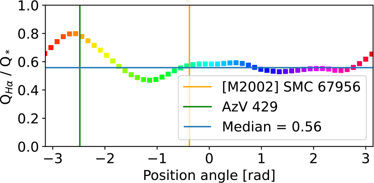
) depends on the selection of angles (Fig. 2) due to the presence of other ionizing sources and a non-isotropic escape of photons.
Observed (Q
 $_{H\alpha}$
) to modeled (
 $Q_*$
) ionizing flux as a function of position angle. Same colors as right panel of Fig 1. Vertical lines indicate position angles of the ionizing stars not considered for
 $Q_*$
.

3. Photoionization models
We model the radial distribution of the LVM emission line fluxes using the c23.02 version of the photoionization code cloudy (Gunasekera et al. Reference Gunasekera, van Hoof, Chatzikos and Ferland2023). We employ the PoWR model as input ionizing radiation. The model considers a spherical distribution of gas with constant density and SMC baseline abundances. The output from cloudy is 1D. To compare the model with LVM data, we calculate the projected surface brightness of the lines using the ray-tracing methodology of Tarantino et al. (Reference Tarantino, Bolatto, Indebetouw, Rubio, Sandstrom, Smith, Stapleton and Wolfire2024). The resulting model predicts most of the observed radial distribution of line ratios. However, it fails to reproduce the surface brightness profiles. This is solved by assuming that the escape of ionizing photons due to covering factor is larger at outer radii. The resulting line ratio and surface brightness profiles are presented in Fig. 3 and Fig. 4, respectively. This model predicts a total escape of ionizing photons of
 $\sim 48\%$
.
Projected radial line ratios of LVM data (points) and photoionization model (line).

Projected radial surface brightness (in erg s
 $^{-1}$
cm
 $^{-2}$
sr
 $^{-1}$
) of LVM data (points) and photoionization model (line). Color represents position angle in Fig 2.

Figure 4 Long description
Panel A: A scatter plot with a fitted line shows the radial surface brightness of the H-beta 4861 angstrom emission line. The x-axis is labeled 'Radius [pc]' and ranges from 0 to 60. The y-axis is labeled 'H-beta 4861 A' and ranges from 0.2 to 1.2 times 10 to the power of -5. Pink points represent observed data, and a blue line represents the model fit. Panel B: A scatter plot with a fitted line shows the radial surface brightness of the [O III] 5007 angstrom emission line. The x-axis is labeled 'Radius [pc]' and ranges from 0 to 60. The y-axis is labeled '[O III] 5007 A' and ranges from 0 to 5 times 10 to the power of -5. Pink points represent observed data, and a blue line represents the model fit. Panel C: A scatter plot with a fitted line shows the radial surface brightness of the [O II] 3726 and 3729 angstrom emission lines. The x-axis is labeled 'Radius [pc]' and ranges from 0 to 60. The y-axis is labeled '[O II] 3726 A + [O II] 3729 A' and ranges from 0 to 3.5 times 10 to the power of -5. Pink points represent observed data, and a blue line represents the model fit. Panel D: A scatter plot with a fitted line shows the radial surface brightness of the [S II] 6716 and 6731 angstrom emission lines. The x-axis is labeled 'Radius [pc]' and ranges from 0 to 60. The y-axis is labeled '[S II] 6716 A + [S II] 6731 A' and ranges from 0 to 2.5 times 10 to the power of -6. Pink points represent observed data, and a blue line represents the model fit.
Acknowledgements
OA acknowledges support from CONAHCyT Beca Nacional para estudios de Posgrado (CVU 1142736). OA and AW acknowledge support from UNAM DGAPA PAPIIT no. IN107725.
Supplementary material
To view supplementary material for this article, please visit https://doi.org/10.1017/S1743921326106553.

 α
 α
 Hα
 Q∗
 Q∗


 −1
 −2
 −1



