2.1 Numerical framework

In this study, the second version of a code called LESOCC2 (large-eddy simulation on curvilinear coordinates), which was first developed at the Institute for Hydromechanics, Karlsruhe Institute of Technology, Germany (Breuer & Rodi Reference Breuer, Rodi, Voke, Kleiser and Chollet1994; Fröhlich & Rodi Reference Fröhlich, Rodi, Launder and Sandham2002), was used for the simulations. The dimensionless LES equations obtained by filtering of the incompressible Navier–Stokes equations can be written as

(2.1) $$\begin{eqnarray}\displaystyle & \displaystyle \frac{\unicode[STIX]{x2202}u_{i}}{\unicode[STIX]{x2202}x_{i}}=0 & \displaystyle\end{eqnarray}$$

(2.2) $$\begin{eqnarray}\displaystyle & \displaystyle \frac{\unicode[STIX]{x2202}u_{i}}{\unicode[STIX]{x2202}t}+\frac{\unicode[STIX]{x2202}}{\unicode[STIX]{x2202}x_{j}}(u_{i}u_{j})=-\frac{\unicode[STIX]{x2202}p}{\unicode[STIX]{x2202}x_{i}}+\frac{\unicode[STIX]{x2202}}{\unicode[STIX]{x2202}x_{j}}\left[\unicode[STIX]{x1D710}\left(\frac{\unicode[STIX]{x2202}u_{i}}{\unicode[STIX]{x2202}x_{j}}+\frac{\unicode[STIX]{x2202}u_{j}}{\unicode[STIX]{x2202}x_{i}}\right)\right]-\frac{\unicode[STIX]{x2202}\unicode[STIX]{x1D70F}_{ij}^{SGS}}{\unicode[STIX]{x2202}x_{j}}, & \displaystyle\end{eqnarray}$$

where $u_{i}$ and $u_{j}$ are the $i$ th and $j$ th components of the resolved instantaneous velocity vector ( $i$ or $j=1$ , 2, 3), $x_{1}$ , $x_{2}$ and $x_{3}$ represent the spatial location vectors in the $x$ , $y$ and $z$ directions, respectively, $p$ is the resolved dimensionless pressure and $\unicode[STIX]{x1D710}$ is the coefficient of kinematic viscosity of the fluid. The subgrid scale (SGS) stress $\unicode[STIX]{x1D70F}_{ij}^{SGS}$ results from filtering of the nonlinear convective fluxes. This term reflects the influence of the subgrid scale turbulence structures on the large eddies. The SGS stress $\unicode[STIX]{x1D70F}_{ij}^{SGS}$ was calculated through an eddy viscosity relation as

(2.3) $$\begin{eqnarray}\displaystyle \unicode[STIX]{x1D70F}_{ij}^{SGS}=-\unicode[STIX]{x1D710}_{SGS}\left(\frac{\unicode[STIX]{x2202}u_{i}}{\unicode[STIX]{x2202}x_{j}}+\frac{\unicode[STIX]{x2202}u_{j}}{\unicode[STIX]{x2202}x_{i}}\right)+\frac{1}{3}\unicode[STIX]{x1D6FF}_{ij}\unicode[STIX]{x1D70F}_{kk}^{SGS}, & & \displaystyle\end{eqnarray}$$

where the SGS viscosity $\unicode[STIX]{x1D710}_{SGS}$ is computed from the dynamic subgrid scale (SGS) model proposed by Germano et al. (Reference Germano, Piomelli, Moin and Cabot1991), $\unicode[STIX]{x1D6FF}_{ij}$ is Kronecker delta.

The governing equations were discretized by the finite-volume method on non-staggered curvilinear grids. Since the outer contour of the roughness elements (hemispheres for impermeable bed and spheres for permeable beds) intersected with the grid lines, the direct forcing immersed boundary method (IBM), originally developed by Peskin (Reference Peskin1972), was incorporated in the LES model. The details of the discretization and the IBM treatment of LESOCC2 are available in Fang et al. (Reference Fang, Bai, He and Zhao2014).

2.2 Averaging approach

The DAM was used to analyse the flows near macro-rough beds. A local instantaneous flow variable $\unicode[STIX]{x1D703}$ can be decomposed into the time–space averaging as

(2.4) $$\begin{eqnarray}\displaystyle \unicode[STIX]{x1D703}(x,y,z,t)=\langle \bar{\unicode[STIX]{x1D703}}\rangle (z)+\tilde{\unicode[STIX]{x1D703}}(x,y,z)+\unicode[STIX]{x1D703}^{\prime }(x,y,z,t), & & \displaystyle\end{eqnarray}$$

where $\tilde{\unicode[STIX]{x1D703}}$ represents the disturbance of the local time-averaged flow parameter $\bar{\unicode[STIX]{x1D703}}$ from the double-averaged (DA) flow parameter $\langle \bar{\unicode[STIX]{x1D703}}\rangle$ (that is, $\tilde{\unicode[STIX]{x1D703}}=\bar{\unicode[STIX]{x1D703}}-\langle \bar{\unicode[STIX]{x1D703}}\rangle$ ), and $\unicode[STIX]{x1D703}^{\prime }$ is the difference of the local instantaneous flow parameter $\unicode[STIX]{x1D703}$ from the local time-averaged flow parameter $\bar{\unicode[STIX]{x1D703}}$ (that is, $\unicode[STIX]{x1D703}^{\prime }=\unicode[STIX]{x1D703}-\bar{\unicode[STIX]{x1D703}}$ ). The spatial averaging used in this study is the intrinsic spatial averaging (Nikora et al. Reference Nikora, McEwan, McLean, Coleman, Pokrajac and Walters2007a ):

(2.5) $$\begin{eqnarray}\displaystyle \langle \bar{\unicode[STIX]{x1D703}}\rangle (z)=\frac{1}{A_{f}}\iint _{A_{f}}\bar{\unicode[STIX]{x1D703}}(x,y,z)\,\text{d}S, & & \displaystyle\end{eqnarray}$$

where $A_{f}$ is the area occupied by the fluid at elevation $z$ within the total area and $\text{d}S$ is an infinitesimal area element. The area $A_{f}$ is typically chosen to be much larger than roughness or flow geometry scales, but smaller than larger geometric features, such as channel curvature and widening or narrowing (Coleman et al. Reference Coleman, Nikora, McLean and Schlicke2007). Since the DAM is applicable for the near-bed flow over and within the flow-roughness-element interface, it enables us to have an insight into the turbulence characteristics of the flow sublayers induced by roughness elements and their link with the main flow. As shown in figure 1, these flow sublayers are the form-induced and interfacial sublayers, together called the roughness sublayer (Dey & Das Reference Dey and Das2012). The form-induced sublayer that occupies the flow zone around the roughness crests is influenced by the individual roughness elements. On the other hand, the interfacial sublayer occupies the flow zone below the form-induced sublayer, where skin friction and form drag appear.

Figure 1.

Flow over a rough, permeable bed showing the flow sublayers.

The DA momentum conservation equation based on the Navier–Stokes equations was developed by Nikora et al. (Reference Nikora, Goring, McEwan and Griffiths2001, Reference Nikora, McEwan, McLean, Coleman, Pokrajac and Walters2007a ) using the time–space averaging procedure. For a uniform, two-dimensional open-channel flow (Giménez-Curto & Corniero Reference Giménez-Curto and Corniero2002; Manes, Pokrajac & McEwan Reference Manes, Pokrajac and McEwan2007; Nikora et al. Reference Nikora, McEwan, McLean, Coleman, Pokrajac and Walters2007a ; Dey & Das Reference Dey and Das2012), the stress balance is given by

(2.6) $$\begin{eqnarray}\displaystyle \langle \bar{\unicode[STIX]{x1D70F}}\rangle =\underbrace{-\unicode[STIX]{x1D70C}\langle \tilde{u} \tilde{w}\rangle }_{\langle \unicode[STIX]{x1D70F}_{f}\rangle }\underbrace{-\unicode[STIX]{x1D70C}\langle \overline{u^{\prime }w^{\prime }}\rangle }_{\langle \unicode[STIX]{x1D70F}_{uw}\rangle }\underbrace{+\unicode[STIX]{x1D70C}\unicode[STIX]{x1D710}\frac{\text{d}\langle \bar{u}\rangle }{\text{d}z}}_{\langle \unicode[STIX]{x1D70F}_{vis}\rangle }+\int _{z}^{h}(f_{v}+f_{p})\,\text{d}z, & & \displaystyle\end{eqnarray}$$

where $\langle \unicode[STIX]{x1D70F}_{f}\rangle$ is the form-induced shear stress (FISS) or dispersive stress (that is, $-\unicode[STIX]{x1D70C}\langle \tilde{u} \tilde{w}\rangle$ ), $\langle \unicode[STIX]{x1D70F}_{uw}\rangle$ is the DA Reynolds shear stress (RSS) (that is, $-\unicode[STIX]{x1D70C}\langle \overline{u^{\prime }w^{\prime }}\rangle$ ), $\langle \unicode[STIX]{x1D70F}_{vis}\rangle$ is the DA viscous shear stress (VSS) (that is, $\unicode[STIX]{x1D70C}\unicode[STIX]{x1D710}(\text{d}\langle \bar{u}\rangle /\text{d}z)$ ), $h$ is the flow depth, and $f_{v}$ and $f_{p}$ are the drag forces induced by viscous and pressure forces, respectively, below the roughness crest ( $z<0$ ). The momentum balance in the main flow produces $\langle \bar{\unicode[STIX]{x1D70F}}\rangle =\langle \unicode[STIX]{x1D70F}_{f}\rangle +\langle \unicode[STIX]{x1D70F}_{uw}\rangle +\langle \unicode[STIX]{x1D70F}_{vis}\rangle$ . Importantly, below the crest, the total drag effects are counted in the total shear stress $\langle \bar{\unicode[STIX]{x1D70F}}\rangle$ computation.

4.1 The double-averaged velocity

A customary parameterization of the log law is

(4.1) $$\begin{eqnarray}\displaystyle \langle \bar{u}\rangle ^{+}=\frac{1}{\unicode[STIX]{x1D705}}\ln \left(\frac{z^{+}+z_{0}^{+}}{k_{s}^{+}}\right), & & \displaystyle\end{eqnarray}$$

where $\langle \bar{u}\rangle ^{+}=\langle \bar{u}\rangle /u_{\ast }$ , $\langle \bar{u}\rangle$ is the DA streamwise velocity, $u_{\ast }$ is the shear velocity, $z^{+}=zu_{\ast }/\unicode[STIX]{x1D710}$ , $z$ is the vertical distance from the crest of the roughness elements, $z_{0}^{+}=z_{0}u_{\ast }/\unicode[STIX]{x1D710}$ , $z_{0}$ is the zero-displacement height, $k_{s}^{+}=k_{s}u_{\ast }/\unicode[STIX]{x1D710}$ , $k_{s}$ is the equivalent roughness height and $\unicode[STIX]{x1D705}$ is equivalent to the von Kármán constant. To plot the data $\langle \bar{u}\rangle ^{+}$ as a function of dimensionless vertical distance $z^{+}+z_{0}^{+}$ for the three cases, a prior estimation of $z_{0}^{+}$ is required. Subsequent determination of $\unicode[STIX]{x1D705}$ and $k_{s}^{+}$ is also essential to fit the data to the log law. The determination of the parameters was done independently, as follows: the data set for $\langle \bar{u}\rangle ^{+}=\langle \bar{u}\rangle /u_{\ast }$ corresponding to $z^{+}+z_{0}^{+}$ was prepared for the analysis. Assuming a very small trial value of $z_{0}^{+}$ , the values of $\unicode[STIX]{x1D705}$ and $z_{0}$ were determined from (4.1) using the regression analysis, and the regression coefficient (RC) was obtained. Then, $z_{0}^{+}$ was incrementally increased by a small value, and $\unicode[STIX]{x1D705}$ and $k_{s}^{+}$ were determined in the same way, until RC reached the maximum. The corresponding values of $z_{0}^{+}$ , $\unicode[STIX]{x1D705}$ and $k_{s}^{+}$ were then determined as $z_{0}^{+}=120.4$ , 422.7 and 974.5, $\unicode[STIX]{x1D705}=0.41$ , 0.34 and 0.32, and $k_{s}^{+}=10.6$ , 107.8 and 295.2 for cases H, S3 and L2, respectively. Figure 4 shows the dimensionless DA streamwise velocity $\langle \bar{u}\rangle ^{+}$ as a function of dimensionless vertical distance $z^{+}+z_{0}^{+}$ for cases H, S3 and L2. Three cases are plotted along with the results of Defina (Reference Defina, Ashworth, Bennett, Best and McLelland1996) and Singh et al. (Reference Singh, Sandham and Williams2007) corresponding to $k_{s}^{+}$ values of 3.4 and 9.6. Earlier studies revealed that the downshift of the time-averaged velocity profile increases with an increase in $k_{s}^{+}$ ( $=k_{s}u_{\ast }/\unicode[STIX]{x1D710}$ ). The $\langle \bar{u}\rangle ^{+}$ -profiles obtained from the LES exhibit a similar trend, confirming the legitimacy of the findings. An increasing trend of $z_{0}^{+}$ with $Re_{K}$ was also obtained by Suga et al. (Reference Suga, Matsumura, Ashitaka, Tominaga and Kaneda2010), which is in conformity with the results obtained from this study. In addition, an inflection point in the $\langle \bar{u}\rangle ^{+}$ -profiles appears at the crest of the roughness elements for these three cases, resulting from a strong flow separation from the crest of the hemispherical or spherical topography (Castro, Cheng & Reynolds Reference Castro, Cheng and Reynolds2006; Coceal et al. Reference Coceal, Dobre, Thomas and Belcher2007). Above the crest, it is apparent that the $\langle \bar{u}\rangle ^{+}$ -profiles preserve the log law, and the logarithmic layer is approximately $z^{+}\in [54:780]$ for case H, $z^{+}\in [80:1400]$ for case S3 and $z^{+}\in [115:1950]$ for case L2. Nezu (Reference Nezu2005) and Suga et al. (Reference Suga, Matsumura, Ashitaka, Tominaga and Kaneda2010) observed that $\unicode[STIX]{x1D705}$ decreases with an increase in permeability Reynolds number $Re_{K}$ , which is also found in the simulated results. On the other hand, below the crest, the $\langle \bar{u}\rangle ^{+}$ -profiles follow a polynomial function having the form $\langle \bar{u}\rangle ^{+}=a+bz^{+}+cz^{+2}+dz^{+3}$ in these three cases, where $a$ , $b$ , $c$ and $d$ are the coefficients. It is in conformity with the results obtained by Sarkar & Dey (Reference Sarkar and Dey2010), Dey & Das (Reference Dey and Das2012) and Sarkar et al. (Reference Sarkar, Papanicolaou and Dey2016).

4.2 The double-averaged Reynolds normal stresses

Figure 5.

Simulated results of (a) DA streamwise Reynolds normal stress, (b) DA spanwise Reynolds normal stress and (c) DA vertical Reynolds normal stress for case H (red dashed line), case S3 (green dashed-dotted line) and case L2 (blue dotted line). Symbol $+$ represents the experimental data with five layers of spheres reported by Manes et al. (Reference Manes, Pokrajac, McEwan and Nikora2009). The thin solid line represents the results of case L2, which were double-averaged by a procedure similar to that of Manes et al. (Reference Manes, Pokrajac, McEwan and Nikora2009). The thick solid line represents the results of the flow over an impermeable smooth bed with the same bulk Reynolds number $Re_{b}=15\,000$ .

Figure 5(a–c) presents the dimensionless DA streamwise, spanwise and vertical Reynolds normal stresses, $(\langle \overline{u^{\prime }u^{\prime }}\rangle ,\langle \overline{v^{\prime }v^{\prime }}\rangle ,\langle \overline{w^{\prime }w^{\prime }}\rangle )\times u_{\ast }^{-2}$ , as a function of dimensionless vertical distance $z/d$ for cases H, S3 and L2. An additional simulation with the same bulk Reynolds number $Re_{b}=15\,000$ was carried out for the flow over an impermeable smooth bed, which was characterized by a coarser grid in the horizontal ( $\unicode[STIX]{x1D6E5}^{x+}=\unicode[STIX]{x1D6E5}^{y+}\approx 16$ ) than case H but which is finer near the smooth wall with $\unicode[STIX]{x1D6E5}^{z+}\approx 1$ . The data for the streamwise and vertical Reynolds normal stresses obtained experimentally by Manes et al. (Reference Manes, Pokrajac, McEwan and Nikora2009) are also plotted along with the simulated results. The bed was covered with five-layer spheres in a cubic pattern in those experiments, which is similar to case L2. As shown in figure 5(a,c), the experimental data plots are in satisfactory agreement with the simulated results of case L2 over the crest. However, below the crest, the profiles of simulated DA streamwise and vertical Reynolds normal stress depart from those of Manes et al. (Reference Manes, Pokrajac, McEwan and Nikora2009), especially for the simulated vertical Reynolds stress values, which are approximately 1.5 times the experimental values. The disagreement is attributed to the different DA procedures. Due to the experimental limitation, the laser light sheet in PIV was placed at two streamwise-oriented vertical planes: one over the top of the spheres and another over their valleys. The spatially averaged portions in the spanwise direction only include these two sections. In this study, we use the total area at an elevation $z$ . If we had adopted the same DA procedure as that adopted by Manes et al. (Reference Manes, Pokrajac, McEwan and Nikora2009), we could have got the solid lines shown in figure 5(a,c), which show a better agreement with the experimental data. It illustrates that the statistics including two sections (top and valley) may underestimate the DA Reynolds normal stress, resulting from the lack of sampling volume in the spanwise direction. In addition, the DA Reynolds normal stresses diminish rapidly inside the permeable wall, becoming negligible below $z/d=-2$ . This indicates that the turbulent flow in the open channel is not influenced by the presence of the solid wall at $z/d=-3$ .

In figure 5(a), the simulated profiles of DA streamwise Reynolds normal stress for rough beds, i.e. case H, case S3 and case L2, collapse on that for impermeable smooth beds for $z/d>1.5$ , substantiating the wall similarity hypothesis (Townsend Reference Townsend1976). In contrast, the profiles of the DA spanwise and vertical normal stresses exhibit less similarity. Breugem et al. (Reference Breugem, Boersma and Uittenbogaard2006) also observed that the DA streamwise Reynolds normal stress preserves similarity in the outer region over a permeable bed, while the similarity disappeared in the spanwise and vertical Reynolds normal stresses. Furthermore, Krogstad & Antonia (Reference Krogstad and Antonia1999) measured boundary-layer flows over rough walls. They reported that the vertical Reynolds normal stress increases significantly and the streamwise Reynolds normal stress remains unchanged as compared to a smooth wall. However, Manes et al. (Reference Manes, Pokrajac, McEwan and Nikora2009) observed that the vertical Reynolds normal stress shows no obvious difference between permeable and impermeable beds over the crest. The reason is attributed to the fact that they used one layer of spheres to represent the impermeable bed and the deep cavities between the spheres to cause larger fluctuations over the bed than for the hemispheres used in this study.

Around the crest, the peaks in the DA streamwise Reynolds stress are lower for the case with higher bed permeability, whereas the peaks are higher for the case with higher bed permeability in the spanwise and vertical Reynolds stresses, which is attributed to the weakening effects of wall-blocking in permeable beds.

Figure 6.

Contours of vertical Reynolds normal stresses and the time-averaged velocity vectors on the $xz$ -plane at $y/d=6.5$ through the centres of hemispheres for (a) case H and large spheres for (b) case S3 and (c) case L2. The dotted line in case S3 shows the periphery of small spheres $(d^{\prime }=0.73d)$ .

Below the crest (within the interfacial layer), the streamwise and spanwise Reynolds normal stresses show much smaller differences among the cases than the vertical Reynolds normal stress, which exhibits fluctuations near $z/d\approx -0.34$ for permeable beds. Interestingly, in case L2, the peaks of the vertical Reynolds normal stresses at $z/d\approx -0.34$ (within the interfacial layer) and $z/d\approx 0.47$ (above the crest) are comparable, illustrating a more pronounced weakening effect of the wall-blocking within the interfacial layer. This weakening effect can be clearly found in figure 6, where the contours of the vertical Reynolds normal stress are shown on the $xz$ -plane at $y/d=6.5$ through the centres of the hemispheres for case H and the large spheres for cases S3 and L2. Above the crests of the spheres, the vertical Reynolds normal stress vanishes rapidly for the three cases, while within the valley formed by the spheres, the fluctuations exhibit different trends. From the time-averaged velocity vectors shown in the insets to figure 6, it is apparent that the vortices shed from the crests of the upstream sphere due to flow separation and then the fluid infiltrate through the interstices of the spheres forming the valleys. As a result of increasing the bed permeability from case S3 to case L2, the shedding gets deeper and causes a more intense vertical Reynolds normal stress. On the other hand, as a result of wall-blocking effects in case H, the vortex shedding is prevented from infiltrating into the bed formed by the hemispheres, leading to a more obvious recirculatory flow within the valley, which decreases the vertical Reynolds normal stress.

The locations which were selected in the line- and point-averaging procedures are shown in figure 7. It is noticeable that the section in $xz$ -plane adopted in figure 6 corresponds to the line over the crest in figure 7. The difference in vertical Reynolds normal stresses between the flow zones near the crests and within the valleys is further exhibited in figure 8. It demonstrates the time- and line-averaged vertical profiles for the wall-normal Reynolds stress in the streamwise direction for each crest and valley side. In addition, the point-averaged vertical profiles are also shown in figure 9.

Figure 7.

Top view of a repeating domain to illustrate the different averaging locations. The red solid line lies over the valley and the blue dashed line lies over the top. The red diamond symbols indicate the valley points and the blue circles the top points.

Above the bed, figure 8(a) shows that the line-averaged Reynolds stress $\langle \overline{w^{\prime }w^{\prime }}\rangle _{l}/u_{\ast }^{2}$ for the top side reaches a higher peak than those for the valley side, which is caused by a strong shear layer shedding from the crest. Below the bed, $\langle \overline{w^{\prime }w^{\prime }}\rangle _{l}/u_{\ast }^{2}$ over the top side decreases more rapidly to zero than that over the valley side, due to the limited space between spheres. However, for permeable beds (i.e. case S3 and case L2) shown in figure 8(b,c), the peaks of $\langle \overline{w^{\prime }w^{\prime }}\rangle _{l}/u_{\ast }^{2}$ over the valley side are higher than those over the top side. The reason is attributed to the fact that as beds become more permeable, the momentum transfer across the bed increases. The wall-blocking effects over the valley side are apparently less than those over the top side. It causes a slightly higher peak of $\langle \overline{w^{\prime }w^{\prime }}\rangle _{l}/u_{\ast }^{2}$ for the valley side above the bed. Vertical Reynolds normal stresses for the valley side are also compared among three cases. As shown in figure 8(d), above the crest ( $z/d>0$ ), the vertical Reynolds normal stresses are higher for the case with higher bed permeability. Below the crest, there exists another peak for permeable beds, especially for case L2. Similar tendencies are also observed in the point-averaged results, as shown in figure 9. Further, the valley points are close to spheres below the crest, while the valley line includes some points located in the diamond-shaped pore space (from the top view, as shown in figure 7), so the increase in the peak value is lower in the valley line-averaged results than the valley point-averaged results, and the corresponding elevations $z/d$ are $-0.5$ and $-0.2$ , respectively.

Figure 8.

Time- and line-averaged vertical profiles of vertical Reynolds normal stresses for (a) case H, (b) case S3 and (c) case L2. For (a,b,c), the red solid line corresponds to the valley and the blue dashed line to the top. For (d), the red dashed line refers to case H, the green dashed-dotted line to case S3 and the blue dotted line to case L2.

Figure 9.

Time and point-averaged vertical profiles of vertical Reynolds normal stresses for (a) case H, (b) case S3 and (c) case L2. For (a,b,c), the red solid line corresponds to the valley and the blue dashed line to the top. For (d), the red dashed line refers to case H, the green dashed-dotted line to case S3 and the blue dotted line to case L2.

4.3 The form-induced normal stresses

Figure 10.

Simulated results of (a) streamwise form-induced normal stress, (b) spanwise form-induced normal stress and (c) vertical form-induced normal stress for case H (red dashed line), case S3 (green dashed-dotted line) and case L2 (blue dotted line).

Figure 10(a–c) depicts the dimensionless streamwise, spanwise and vertical form-induced normal stresses, $(\langle \tilde{u} \tilde{u} \rangle ,\langle \tilde{v}\tilde{v}\rangle ,\langle \tilde{w}\tilde{w}\rangle )\times u_{\ast }^{-2}$ , as a function of dimensionless vertical distance $z/d$ for cases H, S3 and L2. Having compared the results in figures 5 and 10, it is evident that the vertical and spanwise form-induced normal stresses are smaller than the corresponding components of the Reynolds normal stresses. This is consistent with previous experimental studies of a rough wall and canopy (Nikora et al. Reference Nikora, Goring, McEwan and Griffiths2001; Mignot et al. Reference Mignot, Barthelemy and Hurther2009a )). On the other hand, the streamwise form-induced normal stress is comparable to the streamwise Reynolds normal stress, which is characterized by the relatively low submergence (Pokrajac et al. Reference Pokrajac, Campbell, Nikora, Manes and McEwan2007). Within the interfacial layer near $z/d=-0.4$ , the form-induced normal stresses become maximum, exhibiting peaks in their profiles for the three cases. In the $\langle \tilde{u} \tilde{u} \rangle$ -profiles, the peak value of case H (with impermeable bed) is larger than other two cases (with permeable beds), while the peak values in $\langle \tilde{v}\tilde{v}\rangle$ - and $\langle \tilde{w}\tilde{w}\rangle$ -profiles increase with permeability. It can be argued from figure 6 that vortex shedding and recirculation within the valley formed by the spheres cause the spatial fluctuations of velocity for the three cases, leading to peaks near $z/d=-0.4$ . Moreover, the effects of the wall-blocking result in a more stable recirculation in the streamwise direction, causing a relative high magnitude of streamwise form-induced normal stress in case H. However, the vertical and spanwise form-induced normal stresses are enhanced with an increase in permeability. The reason is attributed to the more intense spatial fluctuations of time-averaged flow in those two directions below the crest. In case H (with impermeable bed), the form-induced normal stresses are greater in the near-bed flow zone, where the time-averaged flow is directly influenced by the roughness elements, and they become negligible in the main flow. In contrast, in cases S3 and L2 (with permeable beds), the form-induced normal stresses remain finite even in the main flow. This is triggered by secondary currents, which are discussed in the following section.

4.4 Stress balance and turbulence structure

Figure 11.

(a) DA Reynolds shear stress and (b) stress balance. Total shear stress for case H (red dashed line), case S3 (green dashed-dotted line) and case L2 (blue dotted line); form-induced shear stress for case H (red solid line), case S3 (green solid line) and case L2 (blue solid line). The viscous stresses for three cases are shown in black to distinguish them from the form-induced shear stresses.

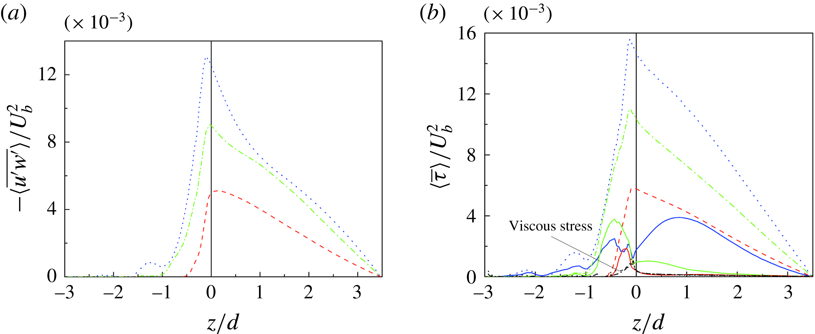
Figure 11(a,b) shows the vertical profiles of the DA Reynolds shear stress $\langle \bar{\unicode[STIX]{x1D70F}}_{uw}\rangle$ ( $=-\unicode[STIX]{x1D70C}\langle \overline{u^{\prime }w^{\prime }}\rangle$ ) and stress balance for the three cases. All the stresses are made dimensionless by $U_{b}^{2}$ , as the profiles of different cases can be separated and shown more clearly. Above the crest ( $z>0$ ), the total shear stress $\langle \bar{\unicode[STIX]{x1D70F}}\rangle$ in (2.6) is balanced by the mean pressure gradient. It has a linear profile for $\langle \bar{\unicode[STIX]{x1D70F}}\rangle (z>0)/(\unicode[STIX]{x1D70C}u_{\ast }^{2})=1-z/h$ (Dey & Das Reference Dey and Das2012; Yuan & Piomelli Reference Yuan and Piomelli2014). As shown in figure 11(a), only for case H (with an impermeable bed) does the DA Reynolds shear stress follow the linear profile away from the roughness elements, while for cases S3 and L2, the shear stresses are damped near $z/d=0.5$ and 1, respectively. Figure 11(b) shows that below the crest, since the time-averaged flow in the vicinity of the spheres is spatially heterogeneous, the form-induced shear stresses grow sharply with a decrease in $z/d$ , attaining peaks at $z/d=-0.2$ , $-0.4$ and $-0.4$ for cases H, S3 and L2, respectively, and then decrease with a further decrease in $z/d$ . The trends of the form-induced shear stresses below the crest are consistent with the results obtained from the previous experimental and numerical studies on macro-rough walls (Mignot et al. Reference Mignot, Barthelemy and Hurther2009a ; Yuan & Piomelli Reference Yuan and Piomelli2014). However, above the crest, only case H (with impermeable bed) follows the conventional trend that $-\langle \tilde{u} \tilde{w}\rangle$ decreases rapidly with an increase in elevation and is negligible in the main flow. The form-induced shear stresses in cases S3 and L2 (with permeable beds) have their peaks near $z/d=0.5$ and 1, respectively, and compensate for the damping of $-\langle \overline{u^{\prime }w^{\prime }}\rangle$ , leading to linear profiles of the total shear stresses from zero at the free surface to a maximum near the crest (figure 11 b). The form-induced shear stresses above the crest for permeable beds are induced by the time-averaged structure of secondary currents. Coleman et al. (Reference Coleman, Nikora, McLean and Schlicke2007) measured the velocity in planes parallel to the centreline over 2D transverse ribs and highlighted the role of secondary currents on momentum transfer. For the momentum balance along the streamwise line, they added the participating secondary current terms (namely, the integral from $z$ to free surface $h$ of $[\unicode[STIX]{x1D70C}\langle \bar{v}\rangle \unicode[STIX]{x2202}\langle \bar{u}\rangle /\unicode[STIX]{x2202}y+\unicode[STIX]{x1D70C}\langle \bar{w}\rangle \unicode[STIX]{x2202}\langle \bar{u}\rangle /\unicode[STIX]{x2202}z+\unicode[STIX]{x1D70C}\unicode[STIX]{x2202}\langle \overline{u^{\prime }w^{\prime }}\rangle /\unicode[STIX]{x2202}y+\unicode[STIX]{x1D70C}\unicode[STIX]{x2202}\langle \tilde{u} \tilde{w}\rangle /\unicode[STIX]{x2202}y]$ ) to (2.6). In this study, the roughness geometry and the flow geometry are periodic due to the sphere arrangement and the boundary conditions are cyclic in the streamwise and spanwise directions. To capture the large scale as well as the detailed flow structures, we adopted spatial averaging in a thin plane parallel to the mean bed, which included all points at an elevation, and so produced $\langle \bar{v}\rangle =\langle \bar{w}\rangle =0$ and $\unicode[STIX]{x2202}(\cdot )/\unicode[STIX]{x2202}y=0$ . Then, the secondary current terms vanish and the effects of the secondary current are represented by the form-induced Reynolds shear stress $\langle \unicode[STIX]{x1D70F}_{f}\rangle =-\unicode[STIX]{x1D70C}\langle \tilde{u} \tilde{w}\rangle$ . The contours of the time-averaged streamwise velocity $\bar{u}/U_{b}$ and the streamlines of the secondary currents ( $\bar{v}$ , $\bar{w}$ ) on the $yz$ -plane at $x/d=12.5$ through the centres of the hemispheres for case H and the large spheres for cases S3 and L2 are shown in figure 12(a–c). It is observed that for case H (with an impermeable bed), the spanwise distribution of $\bar{u}$ is nearly flat above the crest and there are small spanwise vortical flows at the junctions of the surface hemispheres. With an increase in permeability (cases S3 and L2), the spanwise fluctuations of $\bar{u}$ become more obvious and the size of the near-bed cells of the secondary currents increases to approximately $0.5d$ – $3d$ .

Figure 12.

Contours of time-averaged streamwise velocity $\bar{u}/U_{b}$ and streamlines of the secondary currents ( $\bar{v},\bar{w}$ ) on the $yz$ -plane at $x/d=12.5$ through the centres of hemispheres for (a) case H and large spheres for (b) case S3 and (c) case L2. The dotted line in case S3 shows the periphery of small spheres ( $d^{\prime }=0.73d$ ).

To investigate the spanwise turbulence structure in detail, the autocorrelation functions of streamwise and vertical velocity fluctuations, $\unicode[STIX]{x1D70C}_{u^{\prime }u^{\prime }}$ and $\unicode[STIX]{x1D70C}_{w^{\prime }w^{\prime }}$ , are calculated at elevations of $z/d=0$ , 0.5, 1 and 1.5 respectively. They are expressed as

(4.2a,b ) $$\begin{eqnarray}\displaystyle \unicode[STIX]{x1D70C}_{u^{\prime }u^{\prime }}(\unicode[STIX]{x0394}y)=\frac{\displaystyle \int _{0}^{12d}u^{\prime }(y)u^{\prime }(y-\unicode[STIX]{x0394}y)\,\text{d}y}{\displaystyle \int _{0}^{12d}u^{\prime 2}(y)\,\text{d}y},\quad \unicode[STIX]{x1D70C}_{w^{\prime }w^{\prime }}(\unicode[STIX]{x0394}y)=\frac{\displaystyle \int _{0}^{12d}w^{\prime }(y)w^{\prime }(y-\unicode[STIX]{x0394}y)\,\text{d}y}{\displaystyle \int _{0}^{12d}w^{\prime 2}(y)\,\text{d}y},\qquad \; & & \displaystyle\end{eqnarray}$$

where $\unicode[STIX]{x0394}y$ is the spanwise spacing. Figure 13(a–c) presents the autocorrelation functions of the streamwise velocity fluctuations $\unicode[STIX]{x1D70C}_{u^{\prime }u^{\prime }}(\unicode[STIX]{x0394}y/d)$ for cases H, S3 and L2, respectively. The direction of arrows indicates increasing elevation (i.e. $z/d=0$ , 0.5, 1 and 1.5). In essence, the increase in the spanwise spacing of the streamwise velocity fluctuations is characterized by relatively large secondary vortical structures, as was observed by Breugem et al. (Reference Breugem, Boersma and Uittenbogaard2006) from the DNS study. Therefore, for each case, the increasing spanwise spacing with rising elevation illustrates that larger turbulent structures exist in the main flow compared with the near-bed flow zone. In case H, the autocorrelation $\unicode[STIX]{x1D70C}_{u^{\prime }u^{\prime }}$ exhibits a local minimum spanwise spacing of $\unicode[STIX]{x0394}y/d\approx 0.5$ at $z/d=0$ . This local minimum value is associated with the average spanwise distance between low-speed and neighbouring high-speed fluid streaks (Breugem et al. Reference Breugem, Boersma and Uittenbogaard2006). The oscillations in $\unicode[STIX]{x1D70C}_{u^{\prime }u^{\prime }}$ -profiles indicate a periodic fluid streak in the spanwise direction. With an increase in permeability, the local minimum spanwise spacing at $z/d=0$ increases from $\unicode[STIX]{x0394}y/d\approx 0.5$ (case H, with an impermeable bed) to $\unicode[STIX]{x0394}y/d\approx 3$ (case L2, with a highly permeable bed), being consistent with the size of the time-averaged secondary vortices in figure 12. Figure 13(d–f) shows the autocorrelation functions of the vertical velocity fluctuations $\unicode[STIX]{x1D70C}_{w^{\prime }w^{\prime }}(\unicode[STIX]{x0394}y/d)$ for cases H, S3 and L2, respectively. An increasing trend of spanwise spacing with an increase in bed permeability is also observed. Interestingly, with an increase in permeability, the autocorrelation function $\unicode[STIX]{x1D70C}_{w^{\prime }w^{\prime }}$ is less dependent on elevation, indicating that the vertical classification of vortex scale decreases.

Figure 13.

The autocorrelation functions of the streamwise velocity fluctuations $\unicode[STIX]{x1D70C}_{u^{\prime }u^{\prime }}(\unicode[STIX]{x0394}y/d)$ for (a) case H, (b) case S3 and (c) case L2, and the autocorrelation functions of the vertical velocity fluctuations $\unicode[STIX]{x1D70C}_{w^{\prime }w^{\prime }}(\unicode[STIX]{x0394}y/d)$ for (d) case H, (e) case S3 and (f) case L2. The group of curves in a case corresponds to different vertical elevations, increasing in the direction of the arrows as $z/d=0$ (red line), 0.5 (green line), 1 (blue line) and 1.5 (orange line).

Figure 14.

Contours of dimensionless vorticity $\unicode[STIX]{x1D714}_{z}^{+}$ on the $xy$ -plane at $z/d=0.01$ for (a) case H, (b) case S3 and (c) case L2.

Figure 14(a–c) shows the near-bed (at $z/d=0.01$ ) contours of the dimensionless vorticity $\unicode[STIX]{x1D714}_{z}^{+}$ ( $=\unicode[STIX]{x1D714}_{z}\unicode[STIX]{x1D710}/U_{b}^{2}$ , where $\unicode[STIX]{x1D714}_{z}=\unicode[STIX]{x2202}v^{\prime }/\unicode[STIX]{x2202}x-\unicode[STIX]{x2202}u^{\prime }/\unicode[STIX]{x2202}y$ ) on the $xy$ -plane for three cases. The elongated streaky structures, which result from the high- and low-speed fluid streaks and quasi-streamwise vortices, become shredded over the rough and impermeable wall. The longitudinal streamwise vortices become more twisted in case S3. On the other hand, in case L2, the streaky structures are not distinct, and some large-scale intermittent patches, which are considered to be caused by the KH type of instability, are apparent. In addition, strong vertical velocities are prevalent near the permeable bed surface because of the weakening effects of the wall-blocking. The vertical velocities also prevent the development of elongated streaky structures. To quantitatively analyse the statistics of the streamwise scaling, the pre-multiplied spectra at $z/d=0.01$ are shown in figure 15. Spectra were computed as follows: first, the instantaneous spectra $E(k)$ were calculated for each instantaneous profile of velocity fluctuations using a fast Fourier transform technique. Second, all the spectra were averaged at each wavenumber $k_{x}$ in order to decrease the confidence interval pertaining to each spectral estimate. It can be noticed that the spectra are presented in terms of the outer ( $h$ ) scales. Figure 15(a) corresponds to the streamwise velocity. It shows that the spectra for case H in the range $5<k_{x}h<16$ are much higher than those for permeable beds. This means that coherent structures with lengths lying within $0.4{-}1.3h$ are more prevalent over the impermeable bed. For the wall-normal velocity in figure 15(b), the spectra are higher over permeable beds for $k_{x}h>50$ , corresponding to the enhanced wall-normal velocity fluctuations in the small-scale region ( ${<}0.1h$ ). Figure 15 also shows that for large-scale structures lying within $k_{x}h<4$ , the relative magnitudes are inverted as compared to the range $5<k_{x}h<16$ . This is attributed to large-scale coherent structures on the valley side of the permeable beds. We use the isocontours of streamwise autocorrelations to explain this phenomenon.

Figure 15.

Pre-multiplied spectra calculated at $z/d=0.01$ : (a) streamwise velocity and (b) wall-normal velocity in case H (red dashed line), case S3 (green dashed-dotted line) and case L2 (blue dotted line).

The autocorrelation of the streamwise velocity is usually used to quantify the length of streaky structures (Kim, Moin & Moser Reference Kim, Moin and Moser1987; Calmet & Magnaudet Reference Calmet and Magnaudet1997; Breugem et al. Reference Breugem, Boersma and Uittenbogaard2006). For case H, the isocontours of the streamwise autocorrelation of the streamwise velocity and pressure are shown in figures 16 and 17, respectively. It may be noted that this is a one-dimensional correlation, but plotted across the channel. As the bed is characterized by large roughness elements, which are regularly arranged, the spanwise heterogeneity was taken into account. Two typical streamwise planes are adopted, which correspond to the top and the valley. Within the top plane, figure 16(a) shows that the correlation distance is approximately $0.4h$ close to $z/h=0$ , which corresponds to a correlation distance of approximately 400 wall units. The distance is approximately $0.7h$ (i.e. approximately 690 wall units) for the valley side. This behaviour is associated with the presence of streaks. Since the flow through the valley side is not directly blocked by any roughness, the longer distance is found within the valley plane. It is observed that the correlation distance is much shorter over a rough wall than that over a smooth wall, which is typically a length of the order of 1000 wall units (Breugem et al. Reference Breugem, Boersma and Uittenbogaard2006). This means that the wall roughness makes the size of the coherent structures shorter. Furthermore, the correlation distances of pressure on both sides are much shorter than those of the streamwise velocity, as shown in figure 17.

Figure 16.

Isocontours of the autocorrelation of the streamwise velocity as a function of the streamwise spacing $\unicode[STIX]{x0394}x/h$ , shown across the channel for case H. The solid and dashed lines correspond to positive and negative values, respectively. (a) A plane across the top of roughness (i.e. $y/d=6.5$ ). (b) A plane across the valley of roughness (i.e. $y/d=6$ ).

Figure 17.

Isocontours of the autocorrelation of the pressure as a function of the streamwise spacing $\unicode[STIX]{x0394}x/h$ , shown across the channel for case H. The solid and dashed lines correspond to positive and negative values, respectively. (a) A plane across the top of roughness (i.e. $y/d=6.5$ ). (b) A plane across the valley of roughness (i.e. $y/d=6$ ).

Like Breugem et al. (Reference Breugem, Boersma and Uittenbogaard2006), we use the isocontours of the autocorrelations of streamwise velocity and pressure to investigate the turbulence structures, as shown in figures 18 and 19, respectively. Two typical streamwise planes were adopted to explain the relatively large values of spectra lying in the small- and large-wavenumber regions in figure 15. Figure 18(a) corresponds to the top side. It is evident that close to the permeable wall, the correlation distance on the top side of case L2 is much smaller than that on the valley side (i.e. $2h$ ), as shown in figure 18(b), as well as that on the top side over the impermeable bed (i.e. $0.4h$ ), as shown in figure 16(a). The correlation distance close to the wall on the top side is obviously associated with the regularly arranged roughness. It can thus be inferred that turbulent transport across the permeable bed between the roughness increases as compared to the impermeable bed, and the development of elongated structures is prevented. These kinds of small turbulent structures are related to the range with high wavenumbers in the spectra. As for the valley side shown in figure 18(b), turbulent structures as large as $2h$ are found close to $z/h=0$ , which are associated with the peak of the streamwise pre-multiplied spectra $E_{uu}k_{x}$ around $k_{x}h=3$ . Since all the data in the plane $z/d=0.01$ , i.e. all valley sides, top sides and the positions between them, were used to calculate the pre-multiplied spectra, the spectra for a permeable bed are higher in the region of low and high wavenumbers than those for an impermeable bed. In addition, inside the wall, cell-like patterns are observed on the valley side. This feature is also reflected from the streamwise autocorrelation of the pressure in figure 19(b). It corresponds to the presence of the streamwise reciprocal pressure perturbation induced by the KH instability (Kuwata & Suga Reference Kuwata and Suga2016). It can be observed from the streamwise spectrum of the streamwise velocity that the lengths of the KH structures are approximately $2h$ in the streamwise direction. Besides, inside the bed on the top side, as shown in figure 18(a), large-scale structures are found at the same locations on the valley side, but their sizes are limited by the spheres. Additionally, on the valley side, the correlation distance of pressure for case L2 shows a significant increase close to $z/h=0$ as compared to case H.

Figure 18.

Isocontours of the autocorrelation of the streamwise velocity as a function of the streamwise spacing $\unicode[STIX]{x0394}x/h$ , shown across the channel for case L2. The solid and dashed lines correspond to positive and negative values, respectively. (a) A plane across the top of roughness (i.e. $y/d=6.5$ ). (b) A plane across the valley of roughness (i.e. $y/d=6$ ).

Figure 19.

Isocontours of the autocorrelation of the pressure as a function of the streamwise spacing $\unicode[STIX]{x0394}x/h$ , shown across the channel for case L2. The solid and dashed lines correspond to positive and negative values, respectively. (a) A plane across the top of roughness (i.e. $y/d=6.5$ ). (b) A plane across the valley of roughness (i.e. $y/d=6$ ).

The contours of the dimensionless vorticity $\unicode[STIX]{x1D714}_{x}^{+}$ ( $=\unicode[STIX]{x1D714}_{x}\unicode[STIX]{x1D710}/U_{b}^{2}$ , where $\unicode[STIX]{x1D714}_{x}=\unicode[STIX]{x2202}w^{\prime }/\unicode[STIX]{x2202}y-\unicode[STIX]{x2202}v^{\prime }/\unicode[STIX]{x2202}z$ ) on the $yz$ -plane at $x/d=12.5$ through the centres of the hemispheres for case H and the large spheres for cases S3 and L2 are presented in figure 20(a–c). As the permeability increases, the absolute value of vorticity and the spanwise scale of the turbulence structures in the main flow increases, indicating a larger scale of secondary currents. For permeable beds, significant vorticity is also evident within the bed, illustrating that the turbulence structures can also infiltrate the interface of the spherical particles forming the bed.

Figure 20.

Contours of dimensionless vorticity $\unicode[STIX]{x1D714}_{x}^{+}$ on the $yz$ -plane at $x/d=12.5$ through the centres of hemispheres for (a) case H and large spheres for (b) case S3 and (c) case L2. The dotted line in case S3 shows the periphery of small spheres ( $d^{\prime }=0.73d$ ).

Figure 21.

Contours of dimensionless instantaneous streamwise velocity $u/U_{b}$ on the $xz$ -plane at $y/d=6$ through the valleys formed by hemispheres for (a) case H and large spheres for (b) case S3 and (c) case L2. The dotted line shows the periphery of hemispheres or large spheres.

To verify the extent of fluid infiltration and the streamwise flow structures, the contours of dimensionless instantaneous streamwise velocity $u/U_{b}$ on the $xz$ -plane at $y/d=6$ through the valleys formed by the hemispheres for case H and the large spheres for cases S3 and L2 are presented in figure 21(a–c). Figure 21(a) illustrates that for case H (with an impermeable bed), an inrush of high-speed fluid streaks within the interface of the hemispheres exists near $x/d=5$ and an outrush of low-speed fluid streaks also appears near $x/d=9$ , but the extent of infiltration is limited. On the other hand, figure 21(b,c) demonstrates that for cases S3 and L2 (with permeable beds), the flow infiltrates more deeply into the bed, and the extents of infiltration are approximately $d$ and $1.5d$ for cases S3 and L2, respectively. Also, the presence of periodic waves in the streamwise direction indicates that large turbulence structures are getting through the crest level. To quantitatively estimate the flow penetration depth (Brinkman layer thickness) $\unicode[STIX]{x1D6FF}_{u}$ , the profiles of DA velocity $\langle \bar{u}\rangle$ below the crest were analysed. As shown in figure 22, the DA velocity fluctuates from $z/d\approx -1$ to $z/d\approx -2.6$ for case S3 and from $z/d\approx -0.8$ to $z/d\approx -2.6$ for case L2. All velocity values in those zones are averaged to $u_{p}$ ( $u_{p}=0.19u_{\ast }$ for case S3 and $u_{p}=0.34u_{\ast }$ for case L2) with a standard deviation $\unicode[STIX]{x1D70E}$ ( $\unicode[STIX]{x1D70E}=0.04u_{\ast }$ for case S3 and $\unicode[STIX]{x1D70E}=0.06u_{\ast }$ for case L2). The flow penetration depth $\unicode[STIX]{x1D6FF}_{u}$ is taken as the vertical distance between the crest ( $z/d=0$ ) and the point at which the difference between the local DA velocity $\langle \bar{u}\rangle$ and $u_{p}$ decays to 1 % of the DA velocity at the crest ( $u_{c}$ ), i.e. $\langle \bar{u}\rangle _{z=-\unicode[STIX]{x1D6FF}_{u}}=0.01(u_{c}-u_{p})+u_{p}$ . Then, the flow penetration depths $\unicode[STIX]{x1D6FF}_{u}$ are calculated as $-1.09d$ for case S3 and $-1.3d$ for case L2.

Figure 22.

DA streamwise velocity below the crest for case S3 (green dashed-dotted line) and case L2 (blue dotted line). $\unicode[STIX]{x1D6FF}_{u}$ is the flow penetration depth (Brinkman layer thickness), $u_{p}$ is the vertically averaged velocity below the Brinkman layer, $u_{c}$ is the DA velocity at the crest. Values of $\unicode[STIX]{x1D6FF}_{u}$ , $u_{p}$ and $u_{c}$ are only shown for case S3.

The DA Reynolds shear stresses are used to quantify the penetration depth $\unicode[STIX]{x1D6FF}_{rss}$ , which is defined as $-\langle \overline{u^{\prime }w^{\prime }}\rangle _{z=-\unicode[STIX]{x1D6FF}_{rss}}=0.01(-\langle \overline{u^{\prime }w^{\prime }}\rangle )_{max}$ , where $(-\langle \overline{u^{\prime }w^{\prime }}\rangle )_{max}$ is the maximum DA Reynolds shear stress around the crest. Then, the penetration depths of turbulent shear stress $\unicode[STIX]{x1D6FF}_{rss}$ are calculated as $-1.06d$ for case S3 and $-1.52d$ for case L2, as shown in figure 23.

Figure 23.

DA Reynolds shear stress normalized by the maximum shear stress around the crest for case S3 (green dashed-dotted line) and case L2 (blue dotted line). $\unicode[STIX]{x1D6FF}_{rss}$ is the shear stress penetration depth for case S3.

Figure 24.

Contours of dimensionless instantaneous streamwise velocity $u/U_{b}$ and dimensionless Reynolds shear stress $\overline{u^{\prime }w^{\prime }}/u_{\ast }^{2}$ on a $yz$ -plane at $x/d=12$ through the valleys formed by hemispheres for (a) case H and large spheres for (b) case S3 and (c) case L2. The dotted line shows the periphery of hemispheres or large spheres. The enlarged views of the flow zones near the crest are shown in insets.

Figure 24(a–c) presents the contours of dimensionless instantaneous streamwise velocity $u/U_{b}$ and dimensionless Reynolds shear stress $\overline{u^{\prime }w^{\prime }}/u_{\ast }^{2}$ on a $yz$ -plane at $x/d=12$ for cases H, S3 and L2. Vanderwel & Ganapathisubramani (Reference Vanderwel and Ganapathisubramani2015) illustrated that the streamwise continuity of the surface topology was an important factor in the locations of low- and high-momentum pathways. The gap between two neighbouring hemispheres or spheres in the streamwise direction was considered to be $d$ for the three cases. It was less than the length of the separation zone behind a barrier which is known to be approximately $2{-}2.5d$ . So, the closely packed hemispheres or spheres acted like a continuous strip and exhibit a low momentum pathway, which is comparable to previous experiments focusing on the flow over elevated roughness strips. Anderson et al. (Reference Anderson, Barros, Christensen and Awasthi2015) conducted experiments in a wind tunnel and showed that the spanwise-vertical anisotropy of the Reynolds shear stress contributed to the production of time-averaged streamwise vorticity. In case H (with an impermeable bed), the low-velocity zones, which correspond to low-momentum pathways, are in the vicinity of the crests of the hemispheres, whereas in general, the flow between the hemispheres forms relatively high-momentum pathways. In the inset of figure 24(a), it is apparent that the Reynolds shear stress is enhanced over the crests of the hemispheres (low-momentum pathways) and is weakened within the valleys (high-momentum pathways). With the limited width of the spanwise-alternate strips of shear stress, time-averaged secondary currents can only develop near the crest, as shown in figure 12(a). As discussed before, with an increase in permeability, the vertical velocities within the valley formed by the spheres become stronger. This leads to a high shear stress zone as well as a low-momentum pathway within the valley, which connects the adjacent high shear stress zones over the crests of the spheres, as shown in figure 24(b,c). Therefore, as the permeability is higher, a wider extended (connected) high spanwise-alternate shear stress strip is obtained for case S3 and case L2. The extended high shear stress strips act as wider spanwise-alternate roughness strips, causing large time-averaged secondary currents in figure 12(b,c).

4.5 Quadrant analysis of velocity fluctuations

The quadrant analysis of Lu & Willmarth (Reference Lu and Willmarth1973) was employed to identify the presence of coherent structures located at different elevations and to quantify their contributions to the Reynolds shear stress. To perform the quadrant analysis, the velocity fluctuations, $u^{\prime }$ and $w^{\prime }$ , are plotted and divided into four quadrants based on the signs of their instantaneous values. Figure 25(a–l) shows the contours of the turbulent probability density function (PDF) of dimensionless velocity fluctuations, $u^{\prime }/u_{\ast }$ and $w^{\prime }/u_{\ast }$ , at different elevations $z/d$ located on the line of intersection of two vertical planes $x/d=12$ and $y/d=6$ . We choose the location of the points in such a way so that the line of intersection is not blocked by the hemispheres or spheres. In the quadrant analysis, the first quadrant $Q1$ corresponds to $u^{\prime }$ , $w^{\prime }>0$ , called the outward intersection events; the second quadrant $Q2$ to $u^{\prime }<0$ , $w^{\prime }>0$ , called the ejection events; the third quadrant $Q3$ to $u^{\prime }$ , $w^{\prime }<0$ , called the inward intersection events; and the fourth quadrant $Q4$ to $u^{\prime }>0$ , $w^{\prime }<0$ , called the sweep events. Therefore, the ejection events $Q2$ transport a low-momentum fluid upwards away from the bed, while the sweeping events $Q4$ transport a high-momentum fluid downwards towards the bed. The ejection–sweep phenomenon results in intermittent flushing of dead flow that accumulates within the roughness elements (Grass, Stuart & Mansour-Tehrani Reference Grass, Stuart and Mansour-Tehrani1991). Figure 25(a,d) shows that the vertical fluctuations $w^{\prime }$ are relatively small below the crest in case H, and the fluid motion is mainly due to streamwise velocity fluctuations $u^{\prime }$ . As the bed becomes more permeable (from cases 1 to 3), the vertical velocity fluctuations $w^{\prime }$ increase below the crest, which is apparent from figure 25(a–e). This is consistent with figure 6, where the recirculation zone between the hemispheres shows a weak vertical fluid intrusion into the bed, while the fluid intrusion is obviously enhanced over the permeable beds. As the intensity of vertical fluctuations $w^{\prime }$ influences the vertical momentum transport, we can infer that within the valley, the Reynolds shear stress increases with an increase in bed permeability, corresponding to the change of momentum pathways, as shown in figure 24. Moreover, the relatively small vertical fluctuations $w^{\prime }$ result in a weak ejection–sweep phenomenon below the bed. It represents the lack of intermittent flushing and causes a dead-flow zone between the hemispheres in case H. At the crest bed level, the slopes of the PDF in case S3 and case L2 are larger than that in case H, as shown in figure 25(g–i), illustrating larger vertical fluctuations $w^{\prime }$ over permeable beds. With an increase in elevation, statistically significant variations are noticeable between ejection and sweep events for permeable beds. The ejection and sweep events in deep locations are small and almost equal, as shown in figure 25(b,c), indicating an isotropic zone within the interfacial layer. Slightly below the crest, the ejection events are dominant, as shown in figure 25(e,f), transporting low-momentum fluid away from the bed. As the elevation becomes higher, the sweep events seem to be enhanced in figure 25(h,i). Suga et al. (Reference Suga, Matsumura, Ashitaka, Tominaga and Kaneda2010, Reference Suga, Mori and Kaneda2011) and Suga (Reference Suga2016) also revealed that the contribution from sweep events near porous media becomes more dominant, while that from ejection events tends to lose its strength. Further away from bed, the ejection and sweep events are almost identical again, as shown in figure 25(k,l).

Figure 25.

Quadrant analysis of probability density functions (PDFs) of dimensionless velocity fluctuations, $u^{\prime }/u_{\ast }$ and $w^{\prime }/u_{\ast }$ , at different elevations $z/d$ located on the line of intersection of two vertical planes $x/d=12$ and $y/d=6$ . (a–c) $z/d=-0.4$ , (d–f) $z/d=-0.2$ , (g–i) $z/d=0$ and (j–l) $z/d=0.5$ . (a,d,g,j) are case H, (b,e,h,k) are case S3 and (c,f,i,l) are case L2.

4.6 Turbulent kinetic energy budget

The expression for the TKE budget was derived by Raupach, Antonio & Rajagopalan (Reference Raupach, Antonio and Rajagopalan1991) for flow over canopies and Mignot et al. (Reference Mignot, Hurther and Barthelemy2009b ) for flow over macro-roughness (gravel bed). The DA TKE budget for flow over a gravel bed is given by

(4.3) $$\begin{eqnarray}\displaystyle & & \displaystyle \underbrace{-\langle \overline{u_{i}^{\prime }w^{\prime }}\rangle \frac{\unicode[STIX]{x2202}\langle \bar{u}_{i}\rangle }{\unicode[STIX]{x2202}z}}_{P}-\underbrace{\langle \overline{u_{i}^{\prime }u_{j}^{\prime }}\rangle \left\langle \frac{\unicode[STIX]{x2202}\tilde{u} _{i}}{\unicode[STIX]{x2202}x_{j}}\right\rangle }_{P_{m}}-\underbrace{\left\langle u_{i}^{\prime }u_{j}^{\prime }\cdot \frac{\unicode[STIX]{x2202}\tilde{u} _{i}}{\unicode[STIX]{x2202}x_{j}}\right\rangle }_{P_{w}}\nonumber\\ \displaystyle & & \displaystyle \quad =\underset{\substack{ \text{TKE} \\ \text{dissipation}}}{\langle \unicode[STIX]{x1D700}\rangle }+\underbrace{\frac{\unicode[STIX]{x2202}\langle \overline{k^{\prime }w^{\prime }}\rangle }{\unicode[STIX]{x2202}z}}_{F_{k}}+\underbrace{\frac{\unicode[STIX]{x2202}\langle \tilde{k}\tilde{w}\rangle }{\unicode[STIX]{x2202}z}}_{F_{w}}+\underbrace{\frac{1}{\unicode[STIX]{x1D70C}}\frac{\unicode[STIX]{x2202}\langle \overline{p^{\prime }w^{\prime }}\rangle }{\unicode[STIX]{x2202}z}}_{P_{d}}-\underbrace{\unicode[STIX]{x1D710}\frac{\unicode[STIX]{x2202}^{2}\langle k\rangle }{\unicode[STIX]{x2202}z^{2}}}_{v_{d}},\end{eqnarray}$$

where $P$ is the TKE production rate resulting from the DA velocity against the DA shear, $P_{m}$ and $P_{w}$ are the TKE production rates due to velocity fluctuations against the DA shear stress and FISS, respectively, $\unicode[STIX]{x1D700}$ is the TKE dissipation rate, $F_{k}$ and $F_{w}$ are the TKE diffusion and form-induced diffusion rates, respectively, $k^{\prime }=u_{i}^{\prime }u_{i}^{\prime }/2$ , $k=\overline{k^{\prime }}$ , and $P_{d}$ and $v_{d}$ are the pressure energy diffusion and the viscous dissipation rates, respectively. The viscous dissipation rate can be discarded due to its minimal contribution to the TKE budget as compared to other terms over the entire flow depth. Mignot et al. (Reference Mignot, Hurther and Barthelemy2009b ) found that $P_{m}$ and $P_{w}$ were lower than 5 % of the TKE production rate $P$ , while Raupach et al. (Reference Raupach, Antonio and Rajagopalan1991) found that $P_{w}$ was significant below the crest. Lopez & Garcia (Reference Lopez and Garcia1999) obtained the numerical results from a $k$ – $\unicode[STIX]{x1D700}$ model and found that $P_{w}$ could be twice as large as $P$ within the roughness layer. In this study, altogether 18 TKE production rate terms $P_{m}$ and $P_{w}$ (nine for each bed-type-induced terms $P_{m}$ and $P_{w}$ ) were calculated. We found that the sum of them was higher than 10 % of $P$ and they could not be neglected. Moreover, the terms $\langle \overline{u^{\prime }u^{\prime }}\rangle \langle \unicode[STIX]{x2202}\tilde{u} /\unicode[STIX]{x2202}x\rangle$ and $\langle \overline{u^{\prime }w^{\prime }}\rangle \langle \unicode[STIX]{x2202}\tilde{u} /\unicode[STIX]{x2202}z\rangle$ account for more than 85 % of the total $P_{m}$ for three cases, while there is no significant dominance for $P_{w}$ values.

According to the Kolmogorov similarity hypothesis (Kolmogorov Reference Kolmogorov1941), the turbulence statistics in a small-scale universal equilibrium range can be uniquely determined by the kinematic viscosity of the fluid and turbulent dissipation rate as

(4.4) $$\begin{eqnarray}\displaystyle & \displaystyle \langle \unicode[STIX]{x1D700}\rangle =2\unicode[STIX]{x1D710}\langle \overline{s_{ij}s_{ij}}\rangle & \displaystyle\end{eqnarray}$$

(4.5) $$\begin{eqnarray}\displaystyle & \displaystyle s_{ij}=\frac{1}{2}\left(\frac{\unicode[STIX]{x2202}u_{i}^{\prime }}{\unicode[STIX]{x2202}x_{j}}+\frac{\unicode[STIX]{x2202}u_{j}^{\prime }}{\unicode[STIX]{x2202}x_{i}}\right). & \displaystyle\end{eqnarray}$$

Using the three-dimensional velocity fluctuations, the TKE dissipation rate in LES can be calculated more accurately than the experimental data sampling at a point, as done by Mignot et al. (Reference Mignot, Barthelemy and Hurther2009a ).

In dimensionless form, the terms of the TKE budget are expressed as $T_{P}$ , $E_{D}$ , $T_{D}$ , $P_{D}=(P+P_{m}+P_{w},\unicode[STIX]{x1D700},F_{k+}F_{w},P_{d})\times (h/u_{\ast }^{2})$ . The DA pressure energy diffusion rate is calculated as $\langle P_{D}\rangle =\langle T_{P}\rangle -\langle E_{D}\rangle -\langle T_{D}\rangle$ . A comprehensive picture of the variations of the terms of the DA TKE budget in the vicinity of the crest for the three cases is shown in figure 26(a–c). In the three cases, the $\langle T_{P}\rangle$ reaches a maximum value slightly below the crest, $z/d=-0.1$ , which is in conformity with Mignot et al. (Reference Mignot, Barthelemy and Hurther2009a ) and Lopez & Garcia (Reference Lopez and Garcia1999). Below this level, $\langle T_{P}\rangle$ decreases towards a value close to zero for $z/d=-0.5$ , as shown in figure 26(a), and for $z/d=-1$ , as shown in figure 26(b,c). Considering the turbulent diffusion terms, the $\langle T_{D}\rangle$ -profiles possess two peaks for the three cases. By examining the $F_{k}$ - and $F_{w}$ -values, it is observed that the upper peak is mostly attributed to the turbulent diffusion rate $F_{k}$ and the other is to the form-induced diffusion rate $F_{w}$ . Furthermore, $F_{k}$ accounts for more than 80 % of the upper peak for three cases. With an increase in permeability, the contributions from $F_{k}$ are 8 %, 39 % and 50 % of the lower peak of $\langle T_{D}\rangle$ , indicating that the turbulence can reach deeper within the bed.

There are three typical layers defined by the terms of the TKE budget: namely, the equilibrium layer, the form-induced sublayer and the interfacial sublayer. In the equilibrium layer, the TKE production rate nearly balances the turbulent dissipation rate and the diffusion rate is generally found to be negligible (Mignot et al. Reference Mignot, Barthelemy and Hurther2009a ). The layer of high TKE production rates, exceeding the dissipation rates significantly, is called the form-induced sublayer, since the macro-roughness creates a strong, detached mixing-type flow over the crest. The TKE diffusion rates are positive in the form-induced sublayer, transporting TKE upwards and downwards. Towards the bed, in the lower part of the roughness sublayer, called the interfacial sublayer, the flow is characterized by a balance between a low dissipation rate and a low TKE production rate. In figure 26(d), the TKE diffusion rates are compared among the cases, as they can be used to determine the thickness of the form-induced sublayer. The form-induced sublayer is very thin, with an extent from $-0.20d$ to $0.04d$ for case H. For case S3 (with a permeable bed), this layer becomes thicker and the layer extends from $-0.36d$ to $0.25d$ . For case L2 (with a permeable bed, having a permeability greater than that for case S3), the extent of the form-induced sublayer extends from $-0.36d$ to $0.82d$ , indicating a significant influence of permeability on the flow near the bed. Within the interfacial sublayer, the pressure diffusion rate $\langle P_{D}\rangle$ compensates for the turbulent diffusion rate, which is consistent with previous experimental results (Mignot et al. Reference Mignot, Barthelemy and Hurther2009a ).

Figure 26.

The DA TKE budget for (a) case H, (b) case S3 and (c) case L2. $\langle T_{P}\rangle$ (red dashed-dotted line), $\langle E_{D}\rangle$ (green dashed line), $\langle T_{D}\rangle$ (blue dotted line) and $\langle P_{D}\rangle$ (orange solid line). (d) $\langle T_{D}\rangle$ for case H (red line), case S3 (green line) and case L2 (blue line).

4.7 Flow quantities around the crest

As the flow around the crest plays an important role in the transport process and the flow within the bed is difficult to measure experimentally, we choose several typical flow quantities – namely, the flow penetration depth (Brinkman layer thickness), the shear stress penetration depth and the form-induced sublayer thickness – to show their relationships with $Re_{K}$ . The inner scales ( $\unicode[STIX]{x1D710}/u_{\ast }$ ) and mean diameter of sediments ( $d_{p}$ ) are used to normalize these flow quantities. All simulated results over permeable beds (case S1–S5 and case L1–L3) are presented here.

Figure 27.

(a) The DA velocity profiles and (b) DA Reynolds shear stress profiles for eight cases of permeable beds (S1–S5, from black to grey, respectively, and L1–L3, from wine to pink, respectively; lines become lighter with an increase in $Re_{K}$ ).

Figure 27 shows the DA velocity and shear stress profiles for eight cases around the crest. Ghisalberti & Nepf (Reference Ghisalberti and Nepf2002) pointed out that in a turbulent flow over a fairly dense canopy, the inflection of the mean velocity profile was susceptible to the KH instabilities. From figure 27(a), it is apparent that the mean velocity profiles exhibit such an inflection below the crest within permeable beds. According to Rayleigh’s criterion (Drazin & Reid Reference Drazin and Reid1981), it is an essential condition for an inviscid instability. In addition, the mean velocity profiles exhibit a decreasing trend at the crest and an increasing trend within the bed with an increase in $Re_{K}$ . Using the same method as shown in figures 22 and 23, the flow penetration depths $\unicode[STIX]{x1D6FF}_{u}$ and the shear stress penetration depths $\unicode[STIX]{x1D6FF}_{rss}$ for eight permeable cases are calculated and shown in figure 28, which are normalized by $\unicode[STIX]{x1D710}/u_{\ast }$ and $d_{p}$ . The thickness of flow penetration depth (Brinkman layer thickness) can be traditionally described as dependent on the bed permeability (Boudreau Reference Boudreau, Boudreau and Jorgensen2001; Goyeau et al. Reference Goyeau, Lhuillier, Gobin and Velarde2003). However, Goharzadeh, Khalili & Jørgensen (Reference Goharzadeh, Khalili and Jørgensen2005) concluded that the Brinkman layer thickness is of the same order of magnitude as the sediment diameter. In this study, we find a similar conclusion as that of Goharzadeh et al. (Reference Goharzadeh, Khalili and Jørgensen2005). Figure 28(a) demonstrates that the values of the Brinkman layer thickness lie between $0.8d_{p}$ and $1.3d_{p}$ for $Re_{K}$ $O(1{-}10)$ . Moreover, as $Re_{K}$ increases beyond unity, the flow penetration depth normalized by the mean particle diameter becomes deeper. In contrast, for highly permeable beds, the flow penetration depth appears to stay around $1.3d_{p}$ with $Re_{K}$ . This kind of feature may be caused by the methodology used to estimate the critical point $\langle \bar{u}\rangle _{z=-\unicode[STIX]{x1D6FF}_{u}}$ and it can be explained by the magnitude of $u_{p}$ in bed. For a bed with low bed permeability, $u_{p}$ is quite low as a result of the low bed permeability and flow energy ( $u_{\ast }$ ). The change of $u_{\ast }$ mainly affects $u_{c}$ and leads to a decreasing trend of $u_{c}$ and an increasing trend of $u_{p}$ with an increase in $u_{\ast }$ ( $u_{c}$ and $u_{p}$ are both normalized by $u_{\ast }$ ). As the change of $u_{c}$ is more obvious than $u_{p}$ for a bed with low permeability and $u_{\ast }$ (which jointly lead to low $Re_{K}$ ), according to $\langle \bar{u}\rangle _{z=-\unicode[STIX]{x1D6FF}_{u}}=0.01(u_{c}-u_{p})+u_{p}$ , the increase in $u_{\ast }$ over a bed with low permeability leads to a limited increase or slight decrease of the critical velocity $\langle \bar{u}\rangle _{z=-\unicode[STIX]{x1D6FF}_{u}}$ , which results in deeper flow penetration. For a bed with higher $Re_{K}$ , $u_{p}$ increases more significantly than that over a bed with low $Re_{K}$ . The combined effects of an increase in $u_{p}$ and a decrease in $u_{c}$ cause an obvious increase in $\langle \bar{u}\rangle _{z=-\unicode[STIX]{x1D6FF}_{u}}$ , which pushes the critical point closer to the crest. So the flow penetration depth shows a minor difference for high $Re_{K}$ . For the shear stress penetration depth $\unicode[STIX]{x1D6FF}_{rss}$ , it increases to $1.2d_{p}$ over a permeable bed with small $d_{p}$ , i.e. case S1–S5, which is comparable to the Brinkman layer thickness $\unicode[STIX]{x1D6FF}_{u}$ . On the other hand, for a permeable bed with large $d_{p}$ , i.e. L1–L3, the shear stress penetration depth reaches $1.6d_{p}$ , which is caused by the larger pore space between the sphere layers around $z/d=-1$ in cases L1–L3. When the inner scale is adopted in figure 28(b), it shows that except separation behaviour between the cases of different bed configurations, both the flow penetration depth and shear stress penetration depth increase with $Re_{K}$ . For $Re_{K}<20$ , the two kinds of penetration depths are similar, while for $Re_{K}>20$ , the shear stress penetration depth becomes larger than flow penetration depth, with a maximum ratio of 1.4 times at $Re_{K}=109$ . As discussed before, $u_{\ast }$ has some effect on the determination of the critical velocity $\langle \bar{u}\rangle _{z=-\unicode[STIX]{x1D6FF}_{u}}$ ; so we infer that when the penetration depth is normalized by the inner scale, the flow energy (i.e. $u_{\ast }$ ) is considered, which leads to a dependence of $\unicode[STIX]{x1D6FF}^{+}$ on $Re_{K}$ .

Based on the drag force acting within the porous medium (Jackson Reference Jackson1981), Clifton et al. (Reference Clifton, Manes, Rüedi, Guala and Lehning2008) argued that the displacement height is a length scale related to the shear penetration depth. We compare the normalized displacement height $z_{0}/d_{p}$ with the penetration depth $\unicode[STIX]{x1D6FF}/d_{p}$ in figure 28(a), and $z_{0}^{+}$ with $\unicode[STIX]{x1D6FF}^{+}$ in figure 28(b). It shows that the trend of $z_{0}/d_{p}$ with $Re_{K}$ is not consistent with that of $\unicode[STIX]{x1D6FF}/d_{p}$ with $Re_{K}$ . However, when the inner scale was adopted, their trends become more similar. In addition, the ratio of displacement height to penetration depth is approximately 0.46–0.75, which approximates to the theoretical value of 0.5.

Figure 28.

The $Re_{K}$ dependence of flow penetration depth $\unicode[STIX]{x1D6FF}_{u}$ (red dot), shear penetration depth $\unicode[STIX]{x1D6FF}_{rss}$ (blue triangle) and displacement height $z_{0}$ (black cross) normalized by (a) $d_{p}$ and (b) $\unicode[STIX]{x1D710}/u_{\ast }$ . $\unicode[STIX]{x1D6FF}$ represents the penetration depth, i.e. $\unicode[STIX]{x1D6FF}_{u}$ and $\unicode[STIX]{x1D6FF}_{rss}$ . $\unicode[STIX]{x1D6FF}^{+}=\unicode[STIX]{x1D6FF}u_{\ast }/\unicode[STIX]{x1D710}$ and $z_{0}^{+}=z_{0}u_{\ast }/\unicode[STIX]{x1D710}$ .

Based on the criterion that the thickness of the form-induced sublayer $\unicode[STIX]{x1D6FF}_{f}$ can be determined from the elevation at which the TKE diffusion rate $\langle T_{D}\rangle$ attains a small finite value ( $\langle T_{D}\rangle >0$ ), $\unicode[STIX]{x1D6FF}_{f}$ is calculated for all permeable beds. As shown in figure 29(a), $\unicode[STIX]{x1D6FF}_{f}$ normalized by the mean diameter increases around $Re_{K}=1$ and tends to become constant at 1.2 when $Re_{K}$ is $O(10)$ . In figure 29(b), the relationship between $\unicode[STIX]{x1D6FF}_{f}^{+}$ (which is normalized by $\unicode[STIX]{x1D710}/u_{\ast }$ ) and $Re_{K}$ shows similar trends to the penetration depth. In addition, the ratio of the displacement height to the form-induced layer thickness is approximately 0.66–1.28.

Figure 29.

The $Re_{K}$ dependence of the form-induced sublayer thickness $\unicode[STIX]{x1D6FF}_{f}$ (red dot) and displacement height $z_{0}$ (black cross) normalized by (a) $d_{p}$ and (b) $\unicode[STIX]{x1D710}/u_{\ast }$ . $\unicode[STIX]{x1D6FF}_{f}^{+}=\unicode[STIX]{x1D6FF}_{f}u_{\ast }/\unicode[STIX]{x1D710}$ and $z_{0}^{+}=z_{0}u_{\ast }/\unicode[STIX]{x1D710}$ .