



1. Introduction
The dynamics of liquid droplets on solid substrates have been investigated extensively for the past two decades due to their significant connections to a wide range of biological and engineering applications, including heat and mass transfer (Ji & Witelski Reference Ji and Witelski2018), vapour and particle capture (Sadeghpour et al. Reference Sadeghpour, Zeng, Ji, Dehdari Ebrahimi, Bertozzi and Ju2019, Reference Sadeghpour, Oroumiyeh, Zhu, Ko, Ji, Bertozzi and Ju2021), filtration and digital microfluidics (DMF) (Kim Reference Kim2001). These droplet systems often exhibit complex pattern formation rendered by the interactions between the surface tension of the free interface and other physical effects. Fundamental droplet manipulation operations, such as droplet transport, merging and splitting, have been explored experimentally through various mechanisms such as electrodewetting (Chu et al. Reference Chu, Ji, Wang, Kim and Bertozzi2023; Li et al. Reference Li, Ha, Liu, van Dam and Kim2019), electrochemical oxidation (Khoshmanesh et al. Reference Khoshmanesh, Tang, Zhu, Schaefer, Mitchell, Kalantar-Zadeh and Dickey2017) and coalescence-induced propulsion (Jiang et al. Reference Jiang, Feng, O'Donnell, Machado, Choi, Patankar and Park2022). For droplets composed of active matters, such as self-propelled swimmers and driven bio-filaments, recent studies have also explored methods to control these active droplets by manipulating the activity field or evaporation (Shankar, Raju & Mahadevan Reference Shankar, Raju and Mahadevan2022; Chandel, Sivasankar & Das Reference Chandel, Sivasankar and Das2024). Developing robust control mechanisms for droplet dynamics by varying external fields is essential to optimise the manipulation of droplets for practical applications. In this work, we focus on mean field control (MFC) of droplet dynamics in volatile active thin liquid films.
Thin layers of viscous fluids spreading on solid substrates, often referred to as coating flows, have been studied in the context of tear films in human eyes and surface painting processes. When the solid substrate is hydrophobic or non-wetting, the fluid on the substrate spontaneously undergoes a sequence of instabilities and morphological changes, leading to the formation of dry spots and an array of interacting droplets (Glasner & Witelski Reference Glasner and Witelski2003; Ji & Witelski Reference Ji and Witelski2024). This fascinating dewetting phenomenon arises from the interplay of the intermolecular forces between the solid substrate and the fluid and the surface tension of the fluid.
In the limit of low Reynolds number, lubrication theory and thin-film models for free-surface flows have been used widely to model the droplet dynamics (Oron, Davis & Bankoff Reference Oron, Davis and Bankoff1997). Specifically, a classical non-dimensional long-wave thin-film equation can be cast into a gradient dynamics form (Thiele, Archer & Pismen Reference Thiele, Archer and Pismen2016):
 \begin{equation} \frac{\partial h}{\partial t} = \boldsymbol{\nabla}\boldsymbol{\cdot} \left( V_1(h)\boldsymbol{\nabla} \frac{\delta}{\delta h}\mathcal{E}(h)\right) - V_2(h)\frac{\delta}{\delta h}\mathcal{E}(h), \quad \text{on } [0, T] \times\varOmega, \end{equation}
where  $h(t,\boldsymbol {x})$ represents the free surface height of the fluid film,
 $\mathcal {E}$ is an energy functional and
 $V_1(h)\ge 0$ and
 $V_2(h)\ge 0$ are mobility functions associated with mass-conserving and non-mass-conserving contributions to the dynamics. We assume homogeneous Neumann boundary conditions
 $V_1(h)\boldsymbol {\nabla } ({\delta }/{\delta h})\mathcal {E}(h)\boldsymbol {\cdot } \boldsymbol {\nu } = 0$ on the domain boundary
 $\partial \varOmega$, where
 $\boldsymbol {\nu }$ is the outward normal direction on
 $\partial \varOmega$.
For a volatile inactive thin film on a hydrophobic substrate heated or cooled from below (Ajaev & Homsy Reference Ajaev and Homsy2001; Ajaev Reference Ajaev2005b; Ji & Witelski Reference Ji and Witelski2018), vapour condensation or fluid evaporation occurs and leads to non-mass-conserving dynamics. In this case, typical mobility functions in (1.1) take the forms
 \begin{equation} V_1(h) = h^3,\quad V_2(h) = \displaystyle\frac{\gamma}{h + K}, \end{equation}
where  $V_1(h)$ originates from the no-slip boundary condition at the liquid–solid interface,
 $V_2(h)$ characterises the non-mass-conserving liquid evaporation or condensation,
 $\gamma \ge 0$ is a phase change rate and
 $K > 0$ is a kinetic parameter. The energy
 $\mathcal {E}(h)$ is given by
 \begin{equation} \mathcal{E}(h) = \int_{\varOmega} \frac{\alpha^2}{2} |{\boldsymbol{\nabla}{h}}|^2 + U(h)\, {{\rm d}\kern0.7pt x}, \end{equation}
where  $({\alpha ^2}/{2}) |{\boldsymbol {\nabla }{h}}|^2$ represents the contribution of the surface energy of the free interface with
 $\alpha >0$, and
 $U(h)$ is a local free energy relating to the wettability property of the substrate (Bertozzi, Grün & Witelski Reference Bertozzi, Grün and Witelski2001) and the evaporation and condensation effects. When the substrate is partially wetting or hydrophobic, a simple free energy is chosen as
 $U(h)= \frac {1}{3}({\epsilon }/{h})^3 -\tfrac {1}{2}({\epsilon }/{h})^2 - \mathcal {P}_* h,$ and the corresponding disjoining pressure
 $\varPi (h)$ are given by
 \begin{equation} U'(h)=\varPi(h)-\mathcal{P}_*,\quad \varPi(h)= \frac{\epsilon^2}{h^3}\left(1-\frac{\epsilon}{h}\right). \end{equation}
Here, the parameter  $\epsilon$ in
 $\varPi (h)$ sets a positive
 $O(\epsilon )$ lower bound for the liquid height at which the attractive van der Waals forces balance with the short-range Born repulsion. This lower bound also determines the thickness of a precursor layer connecting the droplets, which is commonly assumed in thin-film literature to model the behaviour of the contact line and liquid films on a prewetted layer (Bertozzi et al. Reference Bertozzi, Grün and Witelski2001; Oron & Bankoff Reference Oron and Bankoff2001; Ji & Witelski Reference Ji and Witelski2018; Dukler et al. Reference Dukler, Ji, Falcon and Bertozzi2020). The constant parameter
 $\mathcal {P}_*$ gives the influence of the temperature difference between the liquid film and the surrounding vapour phase. When the film is uniformly heated or cooled from below with a constant temperature imposed at the solid–liquid interface,
 $\mathcal {P}_*$ remains constant in space and time (Ji & Witelski Reference Ji and Witelski2018).
The dynamic pressure  $P$ of the free surface is given by
 \begin{equation} P(h) = \frac{\delta \mathcal{E}}{\delta h}=\varPi(h)-\mathcal{P}_*- \alpha^2{\nabla^2 h}, \end{equation}
where  $\alpha ^2\nabla ^2 h$ gives the linearised curvature of the free surface. We also have the following energy dissipation property:
 \begin{equation} \frac{{\rm d}\mathcal{E}}{{\rm d}t} ={-} \mathcal{I}(h) \le 0, \end{equation}
where the dissipation functional
 \begin{equation} \mathcal{I}(h) := \int_\varOmega \left(V_1(h)|\boldsymbol{\nabla} P(h)|^2 + V_2(h)|P(h)|^2\right)\,{{\rm d}\kern0.7pt x} \end{equation}
is often named the generalised Fisher information functional.
Droplets laden with a suspension of active matter, known as active drops, have also been the focus of many studies in fluid mechanics (Marchetti et al. Reference Marchetti, Joanny, Ramaswamy, Liverpool, Prost, Rao and Simha2013; Maass et al. Reference Maass, Krüger, Herminghaus and Bahr2016). These active droplets consist of internally driven units or self-propelled particles that draw energy from the surrounding and induces active stresses to the background fluids, leading to more complex dynamics and pattern formation (Joanny & Ramaswamy Reference Joanny and Ramaswamy2012). Many studies have focused on the experiments, modelling and fundamentals of active fluids in various applications (Aditi Simha & Ramaswamy Reference Aditi Simha and Ramaswamy2002; Whitfield & Hawkins Reference Whitfield and Hawkins2016; Loisy, Eggers & Liverpool Reference Loisy, Eggers and Liverpool2019; Trinschek et al. Reference Trinschek, Stegemerten, John and Thiele2020). For instance, Adkins et al. (Reference Adkins, Kolvin, You, Witthaus, Marchetti and Dogic2022) experimentally and analytically studied the phase-separating fluid mixtures of active liquid interfaces driven by mechanical activities. Chandel et al. (Reference Chandel, Sivasankar and Das2024) discussed the spontaneous puncturing of active droplets induced by evaporation-driven mass loss. Shankar et al. (Reference Shankar, Raju and Mahadevan2022) studied the optimal transport and control of mass-conserving active drops by controlling the activity. For a comprehensive review, readers are referred to Michelin (Reference Michelin2023). The coupling of non-mass-conserving dynamics and internal dynamics of active drops presents opportunities for designing new control mechanisms. In this work, we consider the MFC of droplet dynamics by controlling the activity field.
Despite the wealth of modelling and analytical results on droplet dynamics, the field of controlling these free surface flows is still in its early stages of development. For instance, researchers have explored reduced-order-model-based control of liquid films governed by the classical Kuramoto–Sivashinsky (KS) equation, employing distributed control across the whole domain (Armaou & Christofides Reference Armaou and Christofides2000; Christofides & Armaou Reference Christofides and Armaou2000; Lee & Tran Reference Lee and Tran2005). Boundary control and optimal control of the KS equation have also been studied in the works of Liu & Krstić (Reference Liu and Krstić2001), Coron & Lü (Reference Coron and Lü2015), Al Jamal & Morris (Reference Al Jamal and Morris2018), Tomlin et al. (Reference Tomlin, Gomes, Pavliotis and Papageorgiou2019), Katz & Fridman (Reference Katz and Fridman2020) and Maghenem, Prieur & Witrant (Reference Maghenem, Prieur and Witrant2022)
The literature on controlling thin-film equations is relatively limited. For example, the work of Wray et al. (Reference Wray, Papageorgiou, Craster, Sefiane and Matar2015) studied the control of evaporating particle laden droplets via an electric field to suppress the ‘coffee-stain’ effect. Klein & Prohl (Reference Klein and Prohl2016) investigated optimal control of a simplified thin-film equation with only the fourth-order term. The work of Samoilova & Nepomnyashchy (Reference Samoilova and Nepomnyashchy2019) considered a linear proportional control for suppressing the Marangoni instability in a thin liquid film evolving on a plane. Cimpeanu, Gomes & Papageorgiou (Reference Cimpeanu, Gomes and Papageorgiou2021) proposed an active control strategy of liquid film flows by incorporating information from reduced-order models. The work of Wray, Cimpeanu & Gomes (Reference Wray, Cimpeanu and Gomes2022) focused on the electrostatic control for thin films underneath an inclined surface. Shankar et al. (Reference Shankar, Raju and Mahadevan2022) studied optimal transport and control of droplets of an active fluid. More recently, Biswal et al. (Reference Biswal, Ji, Elamvazhuthi and Bertozzi2024) studied the optimal boundary control of a thin-film equation describing thin liquid films flowing down a vertical cylinder. The MFC of reaction–diffusion equations (Mielke Reference Mielke2011; Li, Lee & Osher Reference Li, Lee and Osher2022a; Fu, Osher & Li Reference Fu, Osher and Li2023) and regularised conservation laws (Li, Liu & Osher Reference Li, Liu and Osher2022b, Reference Li, Liu and Osher2023) have been studied. In this direction, a recent work of Gao & Qi (Reference Gao and Qi2024) also discussed the control of coherent structures in turbulent flows using mean field games.
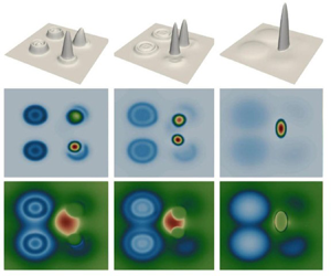
In this study, we demonstrate the application of MFC techniques for manipulating droplet dynamics within the framework of thin-film equations. The objective of MFC is to design and transport the droplets governed by the classical lubrication theory. See figure 1 for an example of the transport and deformation of a droplet on a two-dimensional (2-D) spatial domain from the initial surface height profile  $h_0(x,y)$ to the target height profile
 $h_{T}(x,y)$. To demonstrate the application of optimal control and motivate the design of the MFC formulation, in § 2 we derive a lubrication model for a thin volatile active liquid film, whose dynamics can be controlled through its activity field. We then illustrate the formulation of optimal control of thin-film equations as follows. The constraint is given with the background of original physical dynamics, where the control variables contain both vector field and source terms with the above-mentioned nonlinear mobility functions
 $V_1(h)$ and
 $V_2(h)$. The minimisation is then taken under the kinetic energy originating from the generalised Fisher information functional, adding suitable potential energy and terminal functionals. We then derive two equivalent formulations, for the latter one we develop the minimisation systems of the proposed MFC problems in Proposition 3.6. They can be viewed as the forward–backward controlled systems of thin-film dynamics.
Schematic of the MFC from the initial droplet profile  $h_0(x,y)$ to the target droplet profile
 $h_{T}(x,y)$.

We remark that the proposed MFC problem is motivated by the optimal transport theory (Villani Reference Villani2008). We study the optimal control problem associated with the gradient flow formulation from the thin-film equation in a generalised Wasserstein space. In particular, the control formulation itself is a generalisation of the Benamou–Brenier formula (Benamou & Brenier Reference Benamou and Brenier2000), where we further consider the evolution of fluid dynamics under the thin-film equation as background. The proposed minimisation system is the generalisation of Wasserstein-2-type geodesics.
In simulations, our approach also utilises high-order finite-element computations to achieve this objective. Compared with previous work in Fu et al. (Reference Fu, Osher and Li2023), we remark that the second-order Laplacian term in the dynamic pressure  $P$ in (1.1e) brings additional difficulties in the simulation of proposed MFC problems. We construct several new constraints and Lagrange multipliers associated with primal–dual hybrid gradient (PDHG) methods (Chambolle & Pock Reference Chambolle and Pock2011; Carrillo, Wang & Wei Reference Carrillo, Wang and Wei2023) to handle the constraints associated with the dynamic pressure
 $P$.
The structure of the paper is as follows. In § 2, the model for viscous volatile thin films with an active suspension on a partially wetting substrate is formulated. In § 3, we discuss the MFC of droplet dynamics using the formulated model. In § 4, the high-order space–time finite-element discretisation and its associated PDHG optimisation solver for the proposed MFC problem is presented. Numerical results for the MFC of droplet dynamics using the developed high-order finite-element computations are presented in § 5, followed by concluding remarks and discussion in § 6.
2. Model formulation
In this section, we develop a lubrication model for a thin volatile liquid film laden with an active suspension on a 2-D solid substrate. The liquid properties, including surface tension  $\sigma$, dynamic viscosity
 $\mu$ and density
 $\rho$, are assumed constant. We follow the work of Ajaev (Reference Ajaev2005a) and Ji & Witelski (Reference Ji and Witelski2018) to describe the evaporation and condensation effects using a one-sided model. To incorporate the active suspension into the film dynamics, we follow the approach of Shankar et al. (Reference Shankar, Raju and Mahadevan2022) and consider an active stress that is proportional to the film thickness and describes strong ordering along the
 $x, y$ directions. We show below the derivation of the governing equations and discuss the combined effects of active stresses and non-mass-conserving phenomena.
Following Ajaev & Homsy (Reference Ajaev and Homsy2001), we choose the scales for the system as follows: the characteristic length scale  $\mathscr {L}$ in the
 $x, y$ direction is set as the initial radius of the droplet
 $R_0$. The length scale
 $\mathscr {H}$ in the vertical direction
 $z$ is
 $C^{1/3}R_0$, where
 $C = \mu U/\sigma$ is the capillary number. We assume that the aspect ratio
 $\epsilon = \mathscr {H}/\mathscr {L} = C^{1/3} \ll 1$. The velocity scale in the
 $x, y$ direction is
 $U = k T_s^* / (\rho \mathcal {L} R_0)$, where
 $k$ is the thermal conductivity of the liquid,
 $\mathcal {L}$ is the latent heat of vaporisation per unit mass and
 $T_s^*$ is the saturation temperature. The characteristic vertical velocity is
 $C^{1/3}U$, and the pressure and time scales are given by
 $C^{1/3}\sigma /R_0$ and
 $R_0/U$, respectively. Given a dimensional temperature field
 $T^*$, we express the scaled non-dimensional temperature as
 $T = (T^* - T_s^*)/(C^{2/3}T_s^*)$. In addition, we define the in-plane position
 $\boldsymbol {x} = (x,y)$,
 $\boldsymbol {\nabla }_{\perp } = (\partial _x, \partial _y)$ and the non-dimensional velocity field of the fluid
 $\boldsymbol {u} = (\boldsymbol {u}_{\perp }, w)$, where
 $\boldsymbol {u}_{\perp }$ represents the velocity in the
 $x$ and
 $y$ directions.
Under the lubrication approximation with  $\epsilon \ll 1$, the non-dimensional Stokes equation reduces to the leading-order equations
 \begin{equation} {-}\boldsymbol{\nabla}_{{\perp}} \hat{P} + \frac{\partial^2}{\partial z^2}\boldsymbol{u}_{{\perp}} = 0, \quad -\frac{\partial \hat{P}}{\partial z} = 0, \end{equation}
where  $\hat {P}$ is the non-dimensional pressure of the liquid. At the solid–liquid interface
 $z = 0$, we impose the no-slip and no-penetration boundary conditions
 \begin{equation} \boldsymbol{u}_{{\perp}} = \boldsymbol{0}, \quad w = 0, \quad \text{at } z = 0. \end{equation}
The kinematic boundary condition at the free interface  $z = h(t,\boldsymbol {x})$ is given by
 \begin{equation} \frac{\partial h}{\partial t} = w - \boldsymbol{u}_{{\perp}}\boldsymbol{\cdot} \boldsymbol{\nabla}_{{\perp}} h - J, \quad \text{at } z = h(t, \boldsymbol{x}), \end{equation}
where  $J$ represents the evaporative flux due to evaporation or condensation effects. Using the incompressibility condition
 $\boldsymbol {\nabla }\boldsymbol {\cdot } \boldsymbol {u} = 0$ and boundary conditions (2.2) in the kinematic boundary condition (2.3), we derive
 \begin{equation} \frac{\partial h}{\partial t} + \boldsymbol{\nabla}_{{\perp}} \boldsymbol{\cdot} \left(\int_0^h \boldsymbol{u}_{{\perp}}\,{\rm d}z\right) ={-}J. \end{equation}
We assume that the temperature field  $T(\boldsymbol {x},z)$ across the liquid is quasi-static and is linear in
 $z$ in the leading order under the lubrication approximation, satisfying
 \begin{equation} \frac{\partial^2 T}{\partial z^2} = 0. \end{equation}
This assumption is valid for liquid films under weak evaporation or condensation effects (Burelbach, Bankoff & Davis Reference Burelbach, Bankoff and Davis1988). At the solid–liquid interface, we impose the boundary condition
 \begin{equation} T = \varTheta \quad \text{at } z = 0, \end{equation}
where  $\varTheta$ represents a scaled temperature difference between the solid–liquid interface and the saturation temperature. For
 ${\varTheta } < 0$, we anticipate dominant evaporation dynamics, whereas for large
 $\varTheta > 0$, we expect condensation dynamics. For simplicity, we assume that
 $\varTheta$ is constant in space and time.
At the liquid–air interface, the conservation of energy and the shear stress condition are expressed as
 \begin{equation} J ={-}\frac{\partial T}{\partial z}, \quad \frac{\partial \boldsymbol{u}_{{\perp}}}{\partial z} = 0. \end{equation}
The flux  $J$ is related to the scaled interfacial temperature
 $T^i$ and pressure jump at the liquid–vapour interface by
 \begin{equation} KJ = \gamma (\hat{P}-P_v) + T^i, \end{equation}
where  $P_v$ is the non-dimensional vapour pressure. The constants
 $K$ and
 $\gamma$ are defined by
 $K = (\rho U \sqrt {2{\rm \pi} \bar {R}T_s^*})/(2\rho _v \mathcal {L}C^{1/3})$ and
 $\gamma = \sigma /(\mathcal {L}\rho R_0 C^{1/3})$, where
 $\rho _v$ is the vapour density and
 $\bar {R}$ is the gas constant per unit mass. Solving (2.5)–(2.8) yields the form of the evaporative flux
 \begin{equation} J = \frac{\gamma(\hat{P}-P_v) + \varTheta}{K+h}. \end{equation}
From (2.1) and the boundary conditions (2.2) $_1$ and (2.7)
 $_2$, we obtain
 \begin{equation} \boldsymbol{u}_{{\perp}} = \tfrac{1}{2}(z^2 - 2hz)\boldsymbol{\nabla}_{{\perp}}\hat{P}. \end{equation}
We adopt an active stress tensor  $\boldsymbol {\tau }^a = \hat {\eta } \zeta h (\hat {\boldsymbol {n}}\hat {\boldsymbol {n}} - \boldsymbol {I}/3)$ to account for the contribution of the active suspension to the stress tensor of the liquid, where
 $\hat {\boldsymbol {n}}$ is the orientation field of the active agents in the suspension (Aditi Simha & Ramaswamy Reference Aditi Simha and Ramaswamy2002). Here,
 $\zeta (t, \boldsymbol {x})$ represents the activity field originating from the forcing exerted by the active suspension, and
 $\hat {\eta }$ is a scaling parameter. The activity field
 $\zeta (t, \boldsymbol {x})$ can take either sign: positive and negative values of
 $\zeta$ correspond to contractile and extensile stresses (Joanny & Ramaswamy Reference Joanny and Ramaswamy2012). This model assumes that the active stress depends on the local density of suspension and is applicable to droplets of coherently swimming suspensions and ordered collection of filaments (Loisy et al. Reference Loisy, Eggers and Liverpool2019). We further assume that the rapid orientational relaxation in the vertical direction is negligible, and the orientation field is almost parallel to the substrate with
 $\hat {\boldsymbol {n}} \simeq (n_1(t,\boldsymbol {x}), n_2(t, \boldsymbol {x}), 0)$, where the components
 $n_1$ and
 $n_2$ take the vertically averaged values for the activity strength (Trinschek et al. Reference Trinschek, Stegemerten, John and Thiele2020; Shankar et al. Reference Shankar, Raju and Mahadevan2022).
The total stress in the liquid  $\boldsymbol {\tau } = -(\hat {P}-\varPi (h))\boldsymbol {I} + \mu [\boldsymbol {\nabla } \boldsymbol {u} + (\boldsymbol {\nabla } \boldsymbol {u})^T]+ \boldsymbol {\tau }^a$ incorporates the liquid pressure, the disjoining pressure
 $\varPi (h)$, a viscous stress, and the active stress. The balance of normal stresses at the liquid–vapour interface in the leading order gives
 \begin{equation} \hat{P} = P_v + \varPi(h) - \nabla_{{\perp}}^2 h - \eta h \zeta(t,\boldsymbol{x}) , \end{equation}
where  $\varPi (h)$ is the disjoining pressure,
 $\nabla _{\perp }^2 h$ is the linearised surface tension,
 $P_v$ originates from the stress tensor of the vapour, the parameter
 $\eta = \hat {\eta }/3$, and the vapour recoil is neglected (Oron et al. Reference Oron, Davis and Bankoff1997). Substituting (2.9)–(2.11) into (2.4) yields the evolution equation for
 $h$,
 \begin{align} \frac{\partial h}{\partial t} = \boldsymbol{\nabla}\boldsymbol{\cdot} \left[ h^3\boldsymbol{\nabla} (\varPi(h) - \nabla^2 h - \eta\zeta(t,\boldsymbol{x}) h)\right] - \frac{\gamma\left(\varPi(h) - \nabla^2 h - \eta\zeta(t,\boldsymbol{x}) h - \mathcal{P}_*\right)}{K+h}. \end{align}
Here, we have replaced  $\boldsymbol {\nabla }_{\perp }$ by
 $\boldsymbol {\nabla }$ for simplicity and rescaled the variables by
 $t \to 3t$, and
 $\gamma \to \gamma /3$ to absorb a constant factor of
 $3$ in the mobility function, and the constant parameter
 $\mathcal {P}_*$ is given by
 $\mathcal {P}_* = \varTheta /(3\gamma )$. This model assumes that the active suspension in the droplet is not influenced by the temperature field and neglects Marangoni effects.
In this work, we consider the MFC of the droplet dynamics via the activity field  $\zeta (t, \boldsymbol {x})$. To separate the control variables from the uncontrolled ones, it is convenient to rewrite (2.12) as
 \begin{equation} \frac{\partial h}{\partial t} + \boldsymbol{\nabla} \boldsymbol{\cdot} (V_1(h)\boldsymbol{v}_1) - V_2(h) v_2 = \boldsymbol{\nabla}\boldsymbol{\cdot} \left[ V_1(h)\boldsymbol{\nabla} P(h)\right] - V_2(h)P(h), \end{equation}
where the mobility functions  $V_1(h)$ and
 $V_2(h)$ are defined in (1.1b),
 $\boldsymbol {v}_1$ and
 $v_2$ encode the control variables to the system,
 \begin{equation} \boldsymbol{v}_1 = \boldsymbol{\nabla}(\eta\zeta(t,\boldsymbol{x}) h), \quad v_2 = \eta\zeta(t,\boldsymbol{x}) h, \end{equation}
and  $P(h)$ is the dynamic pressure for the volatile inactive thin-film model defined in (1.1e) with
 $\alpha = 1$. For volatile inactive fluids with
 $\zeta \equiv 0$, the model (2.13) is consistent with the volatile thin-film model (1.1).
The control variable  $\zeta$ enters the system through both a diffusion term and a source term. In the mass-conserving case where
 $\gamma = 0$ (hence
 $V_2\equiv 0$), the activity field
 $\zeta$ affects the local contraction or spreading of the droplet, similar to the setting investigated in Shankar et al. (Reference Shankar, Raju and Mahadevan2022). When
 $\gamma > 0$, the interplay between the activity field and the evaporation/condensation effects can lead to more complex and interesting dynamics. One important quantity is the total mass of the fluid,
 $\mathcal {M}(t)$, and its rate of change due to the non-mass-conserving contributions. By applying Neumann boundary conditions and integrating equation (2.13), we obtain
 \begin{equation} \mathcal{M}(t) = \int_{\varOmega} h\,{\rm d}\boldsymbol{x}, \quad \frac{{\rm d}\mathcal{M}}{{\rm d}t} = \gamma \int_{\varOmega} \frac{\zeta h - P}{K + h}\,{\rm d}\boldsymbol{x}, \end{equation}
which indicates that for  $\gamma > 0$, the mass may locally increase or decrease depending on the local relative importance of the activity field and the pressure, i.e.
 $\zeta h > P$ or
 $\zeta h < P$, respectively.
We remark that the partial differential equation (PDE) (2.13), with varying functional forms of mobility functions, pressure and controls, can be adapted to other types of control problems for both mass-conserving and non-mass-conserving thin-film models. While most existing works on thin-film control (Klein & Prohl Reference Klein and Prohl2016; Samoilova & Nepomnyashchy Reference Samoilova and Nepomnyashchy2019; Shankar et al. Reference Shankar, Raju and Mahadevan2022) focus on the mass-conserving case with  $V_2\equiv 0$, here we illustrate a few examples considered in the literature.
Example 2.1 The work of Klein & Prohl (Reference Klein and Prohl2016) addresses an optimal control problem in the divergence form,
 \begin{equation} \partial_t h = \partial_x (\lambda |h|^{a}\partial_x P) + \partial_x u , \quad P ={-}h_{xx}, \end{equation}
where  $u(t,x)$ is the external control,
 $a > 1$ and
 $\lambda > 0$. This problem characterises the control of thin-film deposition on silicon wafers during electronic chip fabrication. The (2.16) is related to the model (2.13) with
 $V_1 = \lambda |h|^{a}$,
 $V_2 \equiv 0$ and
 $\boldsymbol {v}_1 = -u/V_1$.
Example 2.2 The work of Samoilova & Nepomnyashchy (Reference Samoilova and Nepomnyashchy2019) aimed to suppress the Marangoni instability in a thin film heated from below using a lubrication equation
 \begin{equation} \partial_t h = \boldsymbol{\nabla}\boldsymbol{\cdot} \left[\frac{1}{3}h^3\boldsymbol{\nabla} P + \frac{Ma}{2}h^2\boldsymbol{\nabla} (\varTheta-h)\right], \end{equation}
coupled with a heat transfer equation for the controlled temperature  $\varTheta$. One can rewrite (2.17) into the form of (2.13) by setting
 $V_1 = h^3/3$,
 $V_2 \equiv 0$, and
 $\boldsymbol {v}_1 = ({3Ma}/{2h})\boldsymbol {\nabla }(h-\varTheta )$.
Example 2.3 In the recent work on optimal transport and control of active droplets by Shankar et al. (Reference Shankar, Raju and Mahadevan2022), the active droplet is modelled by
 \begin{equation} \partial_t h = \partial_x \left[\tfrac{1}{3\eta}h^3\partial_x (P -\zeta h)\right], \quad P ={-}\gamma h_{xx}, \end{equation}
where  $\zeta (t,x)$ represents the controllable activity of suspension in the droplet. Again, this problem corresponds to (2.13) with
 $V_1 = h^3/(3\eta )$,
 $V_2\equiv 0$ and
 $\boldsymbol {v}_1 = (\zeta h)_x$.
Remark 2.4 (Rescaling)
For numerical studies throughout the remainder of the paper, we set the computational domain to be a unit square  $\varOmega = [0,1]^2$ for convenience. By rescaling the spatial scale
 $\boldsymbol {x} \to L\boldsymbol {x}$ and the time scale
 $t \to L^2 t$, from (1.1) we obtain the rescaled model for volatile inactive liquid films,
 ${\partial h}/{\partial t} = \boldsymbol {\nabla }\boldsymbol {\cdot }(V_1(h)\boldsymbol {\nabla } P) - V_2(h) P$. Here the rescaled dynamic pressure is given in (1.1e) with the constant
 $\alpha = 1/L$, where
 $L$ is the domain length before rescaling. For the model with the activity field (2.13), to emphasise the importance of the control variables, we introduce the rescaling
 $t \to \beta L^2 t$,
 $\boldsymbol {x} \to L\boldsymbol {x}$ and
 $\gamma \to \gamma /L^2$, where
 $\beta = 1/\eta$. This rescaling leads to the following scaled model:
 \begin{equation} \frac{\partial h}{\partial t} + \boldsymbol{\nabla} \boldsymbol{\cdot} (V_1(h)\boldsymbol{v}_1) - V_2(h) v_2 = \beta\left[\boldsymbol{\nabla}\boldsymbol{\cdot} \left( V_1(h)\boldsymbol{\nabla} P\right) - V_2(h)P\right], \end{equation}
where the vector field  $\boldsymbol {v}_1$ and the source term
 $v_2$ are defined as
 \begin{equation} \boldsymbol{v}_1 = \boldsymbol{\nabla}(\zeta(t,\boldsymbol{x}) h),\quad v_2 = \zeta(t,\boldsymbol{x}) h. \end{equation}
We refer to the system (2.19) as the active control form of the thin-film equation. In the next section, we introduce a MFC model, which selects the active fields  $\boldsymbol {v}_1$ and
 $v_2$ (hence the active field
 $\zeta$) in an optimal manner in certain metrics.
3. MFC of droplet dynamics
This section presents the main formulation of MFC problems for the thin-film equation (1.1). We follow our previous work on MFC for (second-order) reaction–diffusion systems (Fu et al. Reference Fu, Osher, Pazner and Li2024b). A byproduct of our MFC formulation is a new Jordan–Kinderlehrer–Otto (JKO) scheme for the PDE (1.1), which is similar to the variational time implicit scheme discussed in Fu et al. (Reference Fu, Osher and Li2023); see Remark 3.4.
We note that while the general form of the proposed MFC problems has a similar structure to MFC for reaction–diffusion systems considered in our earlier work (Fu et al. Reference Fu, Osher, Pazner and Li2024b), two new challenges emerge for MFC of (1.1). First, the energy functional (1.1c) contains the gradient of the surface height,  $\boldsymbol {\nabla } h$, making (1.1a) a fourth-order PDE. Second, both mobility functions
 $V_1(h)$ and
 $V_2(h)$ are convex functions of
 $h$ (see (1.1b)), which make the MFC problem a non-convex optimisation problem (see Remark 3.2). These new features make the numerical discretisation of the MFC for droplet dynamics significantly more challenging than that for the second-order reaction–diffusion case.
The current work mainly focuses on the MFC formulation of droplet dynamics and its associated high-order finite-element discretisation. We address the first challenge and show how the MFC framework for reaction–diffusion systems developed in Fu et al. (Reference Fu, Osher, Pazner and Li2024b) can be naturally adopted here using additional auxiliary variables. A corresponding high-order space–time finite-element discretisation and its solution procedure using the PDHG method are presented in § 4. We leave theoretical investigations on the (non-)convexity issue of the proposed MFC problem for future work.
3.1. Droplet-dynamics-induced distances and MFCs
The energy dissipation law (1.2) and its associated Fisher information functional (1.3) naturally induce a metric distance between two positive surface heights  $h_0$ and
 $h_1$, as we define in the following.
Definition 3.1 (Distance functional)
Define a distance functional  $\mathrm {Dist}_{V_1,V_2}\colon \mathcal {M}\times \mathcal {M}\rightarrow \mathbb {R}_+$ as below, where the space
 $\mathcal {M} = \{h\in L^1(\varOmega ): h\geq 0\}$. Consider the following optimal control problem:
 \begin{equation} \mathrm{Dist}_{V_1, V_2}(h_0, h_1)^2:=\inf_{h, \boldsymbol{v}_1, v_2}\quad\int_0^1\int_\varOmega \left(|\boldsymbol{v}_1|^2 V_1(h)+ |v_2|^2V_2(h)\right)\,{\rm d}\kern0.7pt x\,{\rm d}t, \end{equation}
where the infimum is taken among  $h(t,x)\colon [0,1]\times \varOmega \rightarrow \mathbb {R}_+$,
 $\boldsymbol {v}_1(t,x)\colon {[0,1]}\times \varOmega \rightarrow \mathbb {R}^d$,
 $v_2(t,x)\colon [0,1]\times \varOmega \rightarrow \mathbb {R}$, such that
 $h$ satisfies a reaction–diffusion-type equation with drift vector field
 $\boldsymbol {v}_1$, drift mobility
 $V_1$, reaction rate
 $v_2$, reaction mobility
 $V_2$, connecting initial and terminal surface heights
 $h_0$,
 ${h_1}\in \mathcal {M}$:
 \begin{equation} \left. \begin{gathered} \partial_t h + \boldsymbol{\nabla}\boldsymbol{\cdot}( V_1(h) \boldsymbol{v}_1)=V_2(h)v_2,\quad (t,x)\in {[0,1]}\times \varOmega,\\ h(0, x)=h_0(x),\quad {h(1,x)=h_1(x)}, \end{gathered} \right\} \end{equation}
with no-flux boundary condition  $V_1(h)\boldsymbol {v}_1\boldsymbol {\cdot }\boldsymbol {\nu }|_{\partial \varOmega }=0$.
Remark 3.2 (On convexity)
We illustrate here that the optimisation problem in Definition 3.1 is a non-convex optimisation problem with a linear constraint. To do so, we introduce variables  $\boldsymbol {m} = V_1(h)\boldsymbol {v}_1$ and
 $s= V_2(h)v_2$, which make the constraint (3.1b) a linear equation:
 $\partial _t h + \boldsymbol {\nabla }\boldsymbol {\cdot }\boldsymbol {m} -s = 0$. Then the objective functional in (3.1a) is
 \begin{equation} \mathcal{L}(h, \boldsymbol{m}, s) = \int_0^1\int_\varOmega \left(\frac{|\boldsymbol{m}|^2}{V_1(h)}+ \frac{|s|^2}{V_2(h)}\right)\,{\rm d}\kern0.7pt x\,{\rm d}t. \end{equation}
From the convexity of mobility functions  $V_1(h)$ and
 $V_2(h)$, we can show that both terms
 ${|\boldsymbol {m}|^2}/{V_1(h)}=\sum _{i=1}^d({|m_i|^2}/{V_1(h)})$ and
 ${s^2}/{V_1(h)}$ fail to be convex in the respective variables. Here the vector
 $\boldsymbol {m} = (m_1,\ldots, m_d)$. In fact, the determinant of the Hessian matrix for the term
 ${|m_1|^2}/{V_1(h)}$ for the variables
 $(h,m_1)$ is
 \begin{equation} \det \begin{bmatrix} \left( 2\dfrac{V_1'(h)^2}{V_1(h)^{3}}- \dfrac{V_1''(h)}{V_1(h)^{2}}\right)|m_1|^2 & -2\dfrac{V_1(h)'}{V_1(h)^2}m_1 & \\ -2\dfrac{V_1(h)'}{V_1(h)^2}m_1 & 2V_1^{{-}1} \end{bmatrix} ={-}2\dfrac{V_1''(h)}{V_1(h)^{3}}|m_1|^2\le 0, \end{equation}
by positivity and convexity of  $V_1(h)$. Hence, the term
 ${|m_1|^2}/{V_1(h)}$ is not convex.
Using the above-defined distance functional and the thin-film equation (1.1), we define the following MFC problem for droplet dynamics.
Definition 3.3 (MFC for droplet dynamics)
Given a time domain  $[0,T]$,
 $T>0$, a potential functional
 $\mathcal {F}\colon \mathcal {M}\rightarrow \mathbb {R}$ and a terminal functional
 $\mathcal {G}\colon \mathcal {M}\rightarrow \mathbb {R}$, consider
 \begin{equation} \inf_{h, \boldsymbol{v}_1, v_2}\int_0^T\left[\int_\varOmega \frac{1}{2}\left(|\boldsymbol{v}_1|^2 V_1(h)+ |v_2|^2V_2(h)\right)\,{{\rm d}\kern0.7pt x} - \mathcal{F}(h)\right]\,{\rm d}t+\mathcal{G}(h(T,\boldsymbol{\cdot})), \end{equation}
where the infimum is taken among  $h(t,x)\colon [0,T]\times \varOmega \rightarrow \mathbb {R}_+$,
 $\boldsymbol {v}_1(t,x)\colon [0,T]\times \varOmega \rightarrow \mathbb {R}^d$ and
 $v_2(t,x)\colon [0,T]\times \varOmega \rightarrow \mathbb {R}$, such that
 \begin{equation} \partial_t h +\boldsymbol{\nabla}\boldsymbol{\cdot}( V_1(h) \boldsymbol{v}_1)-V_2(h)v_2=\beta \left[\boldsymbol{\nabla}\boldsymbol{\cdot}(V_1(h)\boldsymbol{\nabla} P(h))-V_2(h) P(h)\right], \end{equation}
with boundary condition
 \begin{equation} \left.V_1(h) (\boldsymbol{v}_1-\beta\boldsymbol{\nabla} P(h))\boldsymbol{\cdot}\boldsymbol{\nu}\right|_{\partial\varOmega} =0, \end{equation}
and initial surface height  $h(0,\boldsymbol {\cdot }) = h_0$ in
 $\varOmega$. Here
 $\beta \ge 0$ is a non-negative number, which represents the strength of the droplet dynamics (1.1) in the constraint of MFC problem (3.4).
Remark 3.4 (JKO temporal discretisation to (1.1))
In the above definition, if we take  $T=1$,
 $\mathcal {F}=0$ and
 $\mathcal {G}(h) = \Delta t \mathcal {E}(h)$ as in (1.1c), and set parameter
 $\beta = 0$, we obtain a dynamic formulation of the celebrated JKO temporal discretisation scheme Jordan, Kinderlehrer & Otto (Reference Jordan, Kinderlehrer and Otto1998) for the gradient flow (1.1), which is a first-order variational time-implicit discretisation with stepsize
 $\Delta t>0$. See Fu et al. (Reference Fu, Osher and Li2023), Carrillo et al. (Reference Carrillo, Craig, Wang and Wei2022) and Li, Lu & Wang (Reference Li, Lu and Wang2020) for a related discussion on JKO-type discretisations for gradient flows in Wasserstein-type metric spaces.
3.2. MFC reformulations
In this subsection, we focus on reformulations of the MFC problem in Definition 3.3 which will be suitable for a finite-element discretisation.
The first reformulation converts the constraint PDE (3.4b) to a linear constraint by a change of variables. Specifically, introducing the flux function  $\boldsymbol {m}(t,x)\colon [0,T]\times \varOmega \rightarrow \mathbb {R}^d$ and source function
 $s(t, x)\colon [0,T]\times \varOmega \rightarrow \mathbb {R}$, such that
 \begin{equation} \boldsymbol{m}=V_1(h)\left[\boldsymbol{v}_1 -\beta \boldsymbol{\nabla} P(h)\right], \quad s=V_2(h)\left[v_2-\beta P(h)\right], \end{equation}
then the MFC problem in Definition 3.3 is equivalent to the following linearly constrained optimisation problem: given a potential functional  $\mathcal {F}\colon \mathcal {M}\rightarrow \mathbb {R}$ and a terminal functional
 $\mathcal {G}\colon \mathcal {M}\rightarrow \mathbb {R}$, consider
 \begin{align} &\inf_{h, \boldsymbol{m}, s}\int_0^T \int_\varOmega \frac12|\frac{\boldsymbol{m}}{V_1(h)}+\beta\boldsymbol{\nabla} P(h)|^2 V_1(h)\,{\rm d}\kern0.7pt x\,{\rm d}t \nonumber\\ &\qquad +\int_0^T\int_\varOmega \frac12|\frac{s}{V_2(h)}+\beta P(h)|^2V_2(h)\,{\rm d}\kern0.7pt x\,{\rm d}t -\int_0^T\mathcal{F}(h)\,{\rm d}t+\mathcal{G}(h(T,\boldsymbol{\cdot})), \end{align}
where the infimum is taken among functions  $h, \boldsymbol {m}, s$, such that
 \begin{equation} \partial_t h +\boldsymbol{\nabla}\boldsymbol{\cdot} \boldsymbol{m}-s=0 \quad\text{on } [0,T]\times \varOmega, \quad \left.\boldsymbol{m}\boldsymbol{\cdot}\boldsymbol{\nu}\right|_{[0,T]\times\partial\varOmega} =0, h(0,x) = h_0(x). \end{equation}
Expanding the product terms in (3.6), we get
 \begin{align} &\inf_{h, \boldsymbol{m}, s}\int_0^T\!\int_\varOmega \left( \frac{|\boldsymbol{m}|^2}{2V_1(h)} +\frac{|s|^2}{2V_2(h)} \right)+ \beta\left(\boldsymbol{m}\boldsymbol{\cdot}\boldsymbol{\nabla} P(h)+s\boldsymbol{\cdot} P(h) \right) \,{\rm d}\kern0.7pt x\,{\rm d}t \nonumber\\ &\qquad +\int_0^T \int_\varOmega \frac{\beta^2}2 \left(|\boldsymbol{\nabla} P(h)|^2V_1(h) +|P(h)|^2 V_2(h)\right) \,{\rm d}\kern0.7pt x\,{\rm d}t \nonumber\\ &\qquad -\int_0^T\mathcal{F}(h)\,{\rm d}t+\mathcal{G}(h(T,\boldsymbol{\cdot})). \end{align}
Using integration by parts and the constraint (3.7), we have
 \begin{align} & \int_0^T\int_\varOmega \left(\boldsymbol{m}\boldsymbol{\cdot}\boldsymbol{\nabla} P(h)+s\boldsymbol{\cdot} P(h)\right) \,{\rm d}\kern0.7pt x\,{\rm d}t \nonumber\\ &\qquad = \int_0^T \int_\varOmega P(h) \left(-\boldsymbol{\nabla}\boldsymbol{\cdot}\boldsymbol{m}+s \right) \,{\rm d}\kern0.7pt x\,{\rm d}t \nonumber\\ &\qquad = \int_0^T\int_\varOmega P(h) \partial_t h\,{\rm d}\kern0.7pt x\,{\rm d}t= \mathcal{E}(h(T,\boldsymbol{\cdot}))- \mathcal{E}(h_0), \end{align}
where we used the definition of dynamic pressure  $P(h)={\delta \mathcal {E}(h)}/{\delta h}$ in the last step. Combining these derivations and noting that
 $h_0$ is given, we arrive at the following equivalent formulation of the MFC problem in Definition 3.3.
Definition 3.5 (MFC reformulation I)
Consider
 \begin{align} &\inf_{h, \boldsymbol{m}, s} \int_0^T\int_\varOmega \left( \frac{|\boldsymbol{m}|^2}{2V_1(h)} +\frac{|s|^2}{2V_2(h)} \right)\,{\rm d}\kern0.7pt x\,{\rm d}t\nonumber\\ &\qquad +\int_0^T\int_\varOmega \frac{\beta^2}2 \left(|\boldsymbol{\nabla} P(h)|^2V_1(h) +|P(h)|^2 V_2(h)\right) \,{\rm d}\kern0.7pt x\,{\rm d}t \nonumber\\ &\qquad -\int_0^T\mathcal{F}(h)\,{\rm d}t+\mathcal{G}(h(T,\boldsymbol{\cdot})) +\beta \mathcal{E}(h(T,\boldsymbol{\cdot})), \end{align}
where the infimum is taken among  $h$,
 $\boldsymbol {m}$ and
 $s$ satisfying (3.7).
Proposition 3.6 (MFC systems of droplet dynamics)
Let  $(h, \boldsymbol {m}, s)$ be the critical point system of the MFC problem (3.10). Then there exists a function
 $\phi \colon [0, T]\times \varOmega \rightarrow \mathbb {R}$, such that
 \begin{equation} \frac{\boldsymbol{m}(t,x)}{V_1(h(t,x))}=\boldsymbol{\nabla} \phi(t,x),\quad \frac{s(t,x)}{V_2(h(t,x))}=\phi(t,x), \end{equation}
and
 \begin{equation} \left. \begin{gathered}
\partial_th(t,x)
+\boldsymbol{\nabla}\boldsymbol{\cdot}(V_1(h(t,x))\boldsymbol{\nabla}
\phi(t,x))-V_2(h(t,x))\phi(t,x)=0,\\
\partial_t\phi(t,x)+\frac{1}{2}\|\boldsymbol{\nabla}
\phi(t,x)\|^2
V_1'(h(t,x))+\frac{1}{2}|\phi(t,x)|^2V'_2(h(t,x))\\
+\,\frac{\delta}{\delta
h}\left[\mathcal{F}(h)-\frac{\beta^2}{2}\mathcal{I}(h)\right](t,x)=0,
\end{gathered}
\right\}\end{equation}
where  $\mathcal {I}(h)$ is the generalised Fisher information functional given in (1.3), such that
 $$\begin{align} \frac{\delta}{\delta
h}\mathcal{I}(h)&=
\frac{1}{2}(V_1'(h)|\boldsymbol{\nabla}
P(h)|^2+V_2'(h)|P(h)|^2)-\boldsymbol{\nabla}\boldsymbol{\cdot}(V_1(h)\boldsymbol{\nabla}
P(h))\varPi'(h)\nonumber\\ &\quad +\alpha^2\Delta
\boldsymbol{\nabla}\boldsymbol{\cdot}(V_1(h)\boldsymbol{\nabla}
P(h))+\varPi'(h)V_2(h)P(h)-\alpha^2\Delta (P(h)V_2(h)),
\end{align}$$
with initial and terminal time conditions
 \begin{equation} h(0,x)=h_0(x),\quad \phi(T,x)={-}\frac{\delta}{\delta h}\left(\mathcal{G}(h(T,\boldsymbol{\cdot}))+\beta \mathcal{E}(h(T,\boldsymbol{\cdot}))\right). \end{equation}
We remark that a similar MFC formulation and system for reaction–diffusion equation was considered in our earlier work (Fu et al. Reference Fu, Osher and Li2023). We present the derivation of the MFC system (3.12) in Appendix A.
MFC problems and systems are generalisations of Benamou–Brenier formulae in optimal transport (Villani Reference Villani2008). This refers to setting  $\beta =0$,
 $V_1(h)=h$ and
 $V_2(h)=0$. In the context of MFC of droplet dynamics, we need to address additional challenges, in which the dynamic pressure
 $P(h)$ given in (1.1e) involves a second-order Laplacian term. The role of this Laplacian term is well known in lubrication models, and its treatment in both forward simulations (Witelski & Bowen Reference Witelski and Bowen2003) and (boundary) optimal control contexts (Biswal et al. Reference Biswal, Ji, Elamvazhuthi and Bertozzi2024) is well understood. In addition, the treatment of the Laplacian term in controlling free interfaces has been discussed in the context of the KS equation (Tomlin & Gomes Reference Tomlin and Gomes2019) and weighted residual integral boundary layer models (Wray et al. Reference Wray, Cimpeanu and Gomes2022). However, the Laplacian term brings additional difficulties in the computation of the proposed MFC problem using finite-element methods (FEMs). This is from the fact that we need to approximate the forward–backward MFC system (3.12), in which the Laplacian term is enforced in the formulation of generalised Fisher information functional (1.3). We also comment that the dynamic pressure
 $P(h)$ is essential in modellingthe disjoining pressure and surface tension that govern the droplet dynamics. In numerical experiments, we demonstrate that the MFC problem with this pressure term exhibits essential patterns of droplets, including droplet spreading, transport, merging and splitting.
We introduce additional auxiliary variables to further reformulate the MFC problem (3.5). Let  $\boldsymbol {n}(t,x): [0,T]\times \varOmega \rightarrow \mathbb {R}^d$,
 $p(t,x): [0,T]\times \varOmega \rightarrow \mathbb {R}$ and
 $\boldsymbol {q}(t,x): [0,T]\times \varOmega \rightarrow \mathbb {R}^d$ be defined as follows:
 \begin{equation} \boldsymbol{n} = \alpha\boldsymbol{\nabla} h, \quad p ={-}\alpha\boldsymbol{\nabla}\boldsymbol{\cdot} \boldsymbol{n}, \quad \boldsymbol{q} = \alpha \boldsymbol{\nabla} p. \end{equation}
This implies  $p = -\alpha \boldsymbol {\nabla }\boldsymbol {\cdot }(\alpha \boldsymbol {\nabla } h) = -\alpha ^2\nabla ^2h$. Hence, the dynamic pressure
 $P(h)$ and its gradient
 $\boldsymbol {\nabla } P(h)$ can be expressed as follows:
 \begin{equation} P(h) = U'(h)+p, \quad \boldsymbol{\nabla} P(h) = U''(h)\boldsymbol{\nabla} h + \boldsymbol{\nabla} p= \frac1{\alpha}(U''(h)\boldsymbol{n}+\boldsymbol{q}). \end{equation}
Plugging these relations back into the MFC problem (3.10), we obtain the following equivalent reformulation.
Definition 3.7 (MFC reformulation II)
Consider
 \begin{align} &\inf_{h, \boldsymbol{m}, s, \boldsymbol{n}, p, \boldsymbol{q}}\int_0^T\!\int_\varOmega \left( \frac{|\boldsymbol{m}|^2}{2V_1(h)} +\frac{|s|^2}{2V_2(h)}\right)\,{\rm d}\kern0.7pt x\,{\rm d}t\nonumber\\ &\qquad +\int_0^T\!\int_\varOmega \frac{\beta^2}{2} \left(\frac{|U''(h)\boldsymbol{n}+\boldsymbol{q}|^2}{\alpha^2}V_1(h) +|U'(h)+p|^2 V_2(h) \right) \,{\rm d}\kern0.7pt x\,{\rm d}t \nonumber\\ &\qquad -\int_0^T\mathcal{F}(h)\,{\rm d}t+\mathcal{G}(h(T,\boldsymbol{\cdot})) +\beta \int_{\varOmega}\left(U(h(T,x)) + \frac{|\boldsymbol{n}(T,x)|^2}{2}\right)\,{{\rm d}\kern0.7pt x} , \end{align}
where the infimum is taken among  $h$,
 $\boldsymbol {m}$ and
 $s$ satisfying (3.7) and
 $\boldsymbol {n}$,
 $p$ and
 $\boldsymbol {q}$ satisfying (3.14a,b).
To simplify the notation, we collect the variables into a vector
 \begin{equation} \boldsymbol{u} := (h, \boldsymbol{m}, s, \boldsymbol{n}, p, \boldsymbol{q}), \end{equation}
and introduce  $\boldsymbol {u}_T:= (h_T, \boldsymbol {n}_T)$, where
 $h_T:\varOmega \rightarrow \mathbb {R}_+$ is the terminal surface height and
 $\boldsymbol {n}_T:\varOmega \rightarrow \mathbb {R}^d$ the scaled surface height gradient at terminal time. Hence,
 $\boldsymbol {u}(t,x):[0,T]\times \varOmega \rightarrow \mathbb {R}^{3d+3}$ is a space–time function with
 $3d+3$ components and
 $\boldsymbol {u}_T(x):\varOmega \rightarrow \mathbb {R}^{d+1}$ is a spatial function with
 $d+1$ components. We further denote the functionals
 $H(\boldsymbol {u})$ and
 $H_T(\boldsymbol {u}_T)$, such that
 \begin{align} H(\boldsymbol{u}) &:= \frac{|\boldsymbol{m}|^2}{2V_1(h)} +\frac{|s|^2}{2V_2(h)} +\frac{\beta^2}{2\alpha^2} |U''(h)\boldsymbol{n}+\boldsymbol{q}|^2V_1(h) \nonumber\\ &\quad +\frac{\beta^2}{2}|U'(h)+p|^2 V_2(h) - F(h), \end{align}
 \begin{align} H_T(\boldsymbol{u}_T)&:= \beta\left(U(h_T) +\frac{|n_T|^2}{2}\right) +G(h_T), \end{align}
where  $F(h)$ and
 $G(h)$ are density functions for functionals
 $\mathcal {F}$ and
 $\mathcal {G}$, i.e.
 \begin{equation} \mathcal{F}(h) = \int_\varOmega F(h)\,{{\rm d}\kern0.7pt x}, \quad \mathcal{G}(h) = \int_\varOmega G(h)\,{{\rm d}\kern0.7pt x}. \end{equation}
Using this notation, the MFC problem (3.7) takes the following compact form.
Definition 3.8 (MFC problem: compact form)
Consider
 \begin{equation} \inf_{\boldsymbol{u}, \boldsymbol{u}_T}\int_0^T\!\int_\varOmega H(\boldsymbol{u}) \,{\rm d}\kern0.7pt x\,{\rm d}t +\int_{\varOmega}H_T(\boldsymbol{u}_T)\,{{\rm d}\kern0.7pt x}, \end{equation}
subject to the constraints on the space–time domain
 \begin{equation} \left. \begin{aligned} \partial_t h + \boldsymbol{\nabla}\boldsymbol{\cdot}\boldsymbol{m} - s & = 0,\\ -\boldsymbol{n} + \alpha \boldsymbol{\nabla} h & = 0,\\ p + \alpha\boldsymbol{\nabla}\boldsymbol{\cdot}\boldsymbol{n} & = 0,\\ \boldsymbol{q} - \alpha\boldsymbol{\nabla} p & = 0, \end{aligned} \quad\text{on } [0,T]\times\varOmega, \right\} \end{equation}
and the constraints at terminal time
 \begin{equation} \left. \begin{aligned} h(0,\boldsymbol{\cdot}) & = h_0,\\ h(T,\boldsymbol{\cdot}) & = h_T,\\ -\boldsymbol{n}_T + \alpha \boldsymbol{\nabla} h_T & = 0,\\ \end{aligned} \quad\text{on } \varOmega, \right\} \end{equation}
with Neumann boundary condition
 \begin{equation} \boldsymbol{m}\boldsymbol{\cdot}\boldsymbol{\nu} = 0, \quad \text{on }[0,T]\times\partial\varOmega. \end{equation}
Remark 3.9 We note that all the MFC formulations above are mathematically equivalent. Our numerical discretisation, however, will be constructed based on the last formulation in Definition 3.7 or Definition 3.8. It has a form that the constraints are linear PDEs, and the objective function does not involve spatial derivatives. These two properties are crucial for the efficient implementation of the finite-element scheme that we develop in § 4.
Remark 3.10 (On recovering the physics control variable  $\zeta$)

Combining the definition in (3.5a,b) with the optimality conditions (3.11a,b) in Proposition 3.6, we get
 \begin{equation} \boldsymbol{v}_1 - \beta \boldsymbol{\nabla} P(h) = \boldsymbol{\nabla} \phi, \quad v_2-\beta P(h) = \phi. \end{equation}
In particular, this implies that  $\boldsymbol {v}_1$ is a gradient field, and the relation
 $\boldsymbol {v}_1 = \boldsymbol {\nabla } v_2$ holds. Using (2.19b) in § 2 that relate the control variables
 $\boldsymbol {v}_1$ and
 $v_2$ to the activity field
 $\zeta$, we obtain
 \begin{equation} \zeta = \frac{\beta P(h)+\phi}{h} = \frac{\beta(U'(h)+p)+\phi}{h}, \end{equation}
where we used the relation (3.16a,b) in the last equality.
3.3. Saddle-point problem
Finally, we reformulate the constrained optimisation problem in Definition 3.8 into a saddle-point problem using Lagrange multipliers, for which a finite-element discretisation is developed in § 4. We introduce the following four Lagrange multipliers on the space–time domain  $[0,T]\times \varOmega$ for the four equations in (3.21b). They are scalar functions
 $\phi (t,x):[0,T]\times \varOmega \rightarrow \mathbb {R}$,
 $\xi (t,x):[0,T]\times \varOmega \rightarrow \mathbb {R}$, vectorial functions
 $\boldsymbol {\sigma }(t,x):[0,T]\times \varOmega \rightarrow \mathbb {R}^d$,
 $\boldsymbol {\theta }(t,x):[0,T]\times \varOmega \rightarrow \mathbb {R}^d$ and a Lagrange multiplier
 $\boldsymbol {\sigma }_T(x):\varOmega \rightarrow \mathbb {R}^d$ on the spatial domain (at terminal time):
 \begin{equation} \left. \begin{gathered} \partial_t h + \boldsymbol{\nabla}\boldsymbol{\cdot}\boldsymbol{m} - s = 0 \longleftrightarrow \phi,\\ -\boldsymbol{n} + \alpha \boldsymbol{\nabla} h = 0 \longleftrightarrow \boldsymbol{\sigma},\\ p + \alpha\boldsymbol{\nabla}\boldsymbol{\cdot}\boldsymbol{n} = 0 \longleftrightarrow \xi,\\ \boldsymbol{q} - \alpha\boldsymbol{\nabla} p = 0 \longleftrightarrow \boldsymbol{\theta},\\ -\boldsymbol{n}_T + \alpha \boldsymbol{\nabla} h_T = 0 \longleftrightarrow \boldsymbol{\sigma}_T. \end{gathered} \right\} \end{equation}
Then the MFC problem (3.8) can be formulated as the following saddle-point problem:
 \begin{align} &\inf_{\boldsymbol{u}, \boldsymbol{u}_T} \sup_{\boldsymbol{\varPhi}, \boldsymbol{\sigma}_T} \int_0^T\int_\varOmega H(\boldsymbol{u}) \,{\rm d}\kern0.7pt x\,{\rm d}t +\int_{\varOmega}H_T(\boldsymbol{u}_T)\,{{\rm d}\kern0.7pt x}\nonumber\\ &\qquad +\int_0^T\int_\varOmega \left[(\partial_t h + \boldsymbol{\nabla}\boldsymbol{\cdot}\boldsymbol{m} - s)\phi +(-\boldsymbol{n} + \alpha\boldsymbol{\nabla} h)\boldsymbol{\cdot}\boldsymbol{\sigma}\right]\,{\rm d}\kern0.7pt x\,{\rm d}t\nonumber\\ &\qquad +\int_0^T\int_\varOmega \left[(p + \alpha\boldsymbol{\nabla}\boldsymbol{\cdot}\boldsymbol{n})\xi+ (\boldsymbol{q}-\alpha\boldsymbol{\nabla} p)\boldsymbol{\cdot}\boldsymbol{\theta} \right] \,{\rm d}\kern0.7pt x\,{\rm d}t\nonumber\\ &\qquad +\int_\varOmega (-\boldsymbol{n}_T + \alpha\boldsymbol{\nabla} h_T)\boldsymbol{\cdot}\boldsymbol{\sigma}_T \,{{\rm d}\kern0.7pt x}, \end{align}
with the following boundary and initial/terminal conditions
 \begin{equation} h(0,\boldsymbol{\cdot}) = h_0, \ \ h(T,\boldsymbol{\cdot}) = h_T, \quad \text{in }\varOmega, \quad\text{and}\quad \boldsymbol{m}\boldsymbol{\cdot}\boldsymbol{\nu} = 0,\quad \text{on }[0,T]\times\partial\varOmega. \end{equation}
Here  $\boldsymbol {\varPhi } = (\phi, \xi, \boldsymbol {\sigma }, \boldsymbol {\theta })$.
Next, applying integration by parts on the above saddle-point problem to move all derivatives of  $\boldsymbol {u}$ to the dual variables
 $\boldsymbol {\varPhi }$, and using the initial and boundary conditions, we obtain
 \begin{align} &\inf_{\boldsymbol{u}, \boldsymbol{u}_T} \sup_{\boldsymbol{\varPhi}, \boldsymbol{\sigma}_T}\int_0^T\int_\varOmega H(\boldsymbol{u}) \,{\rm d}\kern0.7pt x\,{\rm d}t +\int_{\varOmega}H_T(\boldsymbol{u}_T)\,{{\rm d}\kern0.7pt x}\nonumber\\ &\qquad +\int_0^T\int_\varOmega \left[-( h \partial_t\phi+ \boldsymbol{m}\boldsymbol{\cdot}\boldsymbol{\nabla}\phi + s\phi) -(\boldsymbol{n}\boldsymbol{\cdot}\boldsymbol{\sigma} + \alpha h\boldsymbol{\nabla}\boldsymbol{\cdot}\boldsymbol{\sigma})\right]\,{\rm d}\kern0.7pt x\,{\rm d}t\nonumber\\ &\qquad +\int_0^T\int_\varOmega \left[(p \xi- \alpha\boldsymbol{n}\boldsymbol{\cdot}\boldsymbol{\nabla} \xi)+ (\boldsymbol{q}\boldsymbol{\cdot}\boldsymbol{\theta}+\alpha p\boldsymbol{\nabla} \boldsymbol{\cdot}\boldsymbol{\theta}) \right] \,{\rm d}\kern0.7pt x\,{\rm d}t\nonumber\\ &\qquad +\int_\varOmega\left[-(\boldsymbol{n}_T \boldsymbol{\cdot}\boldsymbol{\sigma}_T+ \alpha h_T \boldsymbol{\nabla}\boldsymbol{\cdot}\boldsymbol{\sigma}_T) +h_T\phi(T, x)-h_0\phi(0, x)\right] \,{{\rm d}\kern0.7pt x}. \end{align}
In the above formulation, we assume the Lagrange multipliers  $\boldsymbol {\sigma }$,
 $\xi$ and
 $\boldsymbol {\theta }$ satisfy the following Neumann boundary conditions:
 \begin{equation} \boldsymbol{\sigma}\boldsymbol{\cdot}\boldsymbol{\nu} = 0,\quad \boldsymbol{\nabla}{\xi}\boldsymbol{\cdot}\boldsymbol{\nu} = 0, \quad \boldsymbol{\theta}\boldsymbol{\cdot}\boldsymbol{\nu} = 0, \quad \text{on }[0,T]\times\partial\varOmega. \end{equation}
The saddle-point problem (3.27) is the final form of our MFC problem that is discretised in the next section. The variational structure of this problem makes the FEM an ideal candidate for such a problem. We close this section with a discussion on the proper function spaces for the primal variables  $\boldsymbol {u}$ and
 $\boldsymbol {u}_T$ and dual variables
 $\boldsymbol {\varPhi }$ and
 $\boldsymbol {\sigma }_T$ in (3.27) which makes the integrals in (3.27) valid. The spaces are given as follows:
 \begin{align} \boldsymbol{u}&\in \left\{
\boldsymbol{v}\in [L^2([0,T]\times \varOmega)]^{3d+3}:\quad
\int_0^T\int_{\varOmega}H(\boldsymbol{v})\,{\rm d}\kern0.7pt x\,{\rm
d}t <{+}\infty,\right.\nonumber\\ &\left.\qquad \text{first
component of }\boldsymbol{v} \text{ is non-negative}
\vphantom{\int_{\varOmega}}\right\},
\end{align}
 \begin{align}
\boldsymbol{u}_T&\in \left\{ \boldsymbol{v}_T\in
[L^2(\varOmega)]^{d+1}:\quad
\int_{\varOmega}H_T(\boldsymbol{v}_T)\,{{\rm d}\kern0.7pt x}
<{+}\infty,\right.\nonumber\\ & \left.\qquad \text{first
component of }\boldsymbol{v}_T \text{ is non-negative}
\vphantom{\int_{\varOmega}}\right\},
\end{align}
 \begin{align} \boldsymbol{\varPhi}&\in V_{\phi}\times \boldsymbol{V}_{\sigma}\times {V}_{\xi}\times \boldsymbol{V}_{\theta}, \qquad \boldsymbol{\sigma}_T\in H_0(\mathrm{div}; \varOmega), \end{align}
where
 $$\begin{gather} V_{\phi}= H^1([0,T]\times\varOmega), \end{gather}$$
 $$\begin{gather}\boldsymbol{V}_{\sigma}=\boldsymbol{V}_{\theta}= L^2([0,T])\otimes H_0(\mathrm{div};\varOmega), \end{gather}$$
 $$\begin{gather}{V}_{\xi}= L^2([0,T])\otimes H_0^1(\varOmega). \end{gather}$$
Here we use the usual definition of Sobolev spaces
 $$\begin{gather} L^2(\varOmega):=\{v:\varOmega\rightarrow \mathbb{R}: \;\;\int_{\varOmega}|v|^2dx <{+}\infty\}, \end{gather}$$
 $$\begin{gather}H^1(\varOmega):=\{v\in L^2(\varOmega): \boldsymbol{\nabla} v \in [L^2(\varOmega)]^d\}, \end{gather}$$
 $$\begin{gather}H(\mathrm{div}; \varOmega):=\{\boldsymbol{v}\in [L^2(\varOmega)]^d: \boldsymbol{\nabla} \boldsymbol{\cdot} \boldsymbol{v} \in L^2(\varOmega)\}. \end{gather}$$
Moreover,  $H^1_0(\varOmega )$ is the subspace of
 $H^1(\varOmega )$ with a zero boundary condition, and
 $H_0(\mathrm {div}; \varOmega )$ is the subspace of
 $H(\mathrm {div}; \varOmega )$ with a zero boundary condition on the normal direction.
4. High-order discretisations and optimisation algorithms
This section presents the high-order spatial-time finite-element discretisation and its associated PDHG optimisation solver for the proposed MFC saddle-point problem (3.27).
4.1. The high-order finite-element scheme
We first partition the spatial domain  $\varOmega$ into a spatial mesh
 $\varOmega _h=\{K_\ell \}_{\ell =1}^{N_S}$ with
 $N_S$ elements where each element
 $K_{\ell }$ is assumed to be a mapped hypercube in
 $\mathbb {R}^d$, and the temporal domain
 $[0,T]$ into a temporal mesh
 $I_h=\{I_j\}_{j=1}^{N_T}$ with
 $N_T$ segments. Denote the space–time mesh as
 $\varOmega _{T,h}=I_h\otimes \varOmega _h$. The function spaces in (3.29) for the saddle-point problem (3.27) indicate natural discretisation spaces for the primal and dual variables. In particular, we use the following conforming finite-element spaces to discretise the dual variables
 $\boldsymbol {\varPhi }$ and
 $\boldsymbol {\sigma }_T$:
 $$\begin{gather} V_{\phi,h}^{k+1} = \{\psi\in V_{\phi}: v|_{I_j\times K_\ell} \in Q^{k+1}(I_j)\otimes Q^{k+1}(K_\ell)\quad \forall j, \ell\}, \end{gather}$$
 $$\begin{gather}\boldsymbol{V}_{\sigma,h}^k = \{\boldsymbol{\tau}\in \boldsymbol{V}_{\sigma}: \boldsymbol{\tau}|_{I_j\times K_\ell} \in Q^k(I_j)\otimes RT^k(K_\ell)\quad \forall j, \ell\}, \end{gather}$$
 $$\begin{gather}{V}_{\xi,h}^{k,k+1} = \{q\in \boldsymbol{V}_{\xi}: q|_{I_j\times K_\ell} \in Q^k(I_j)\otimes Q^{k+1}(K_\ell)\quad\forall j, \ell\}, \end{gather}$$
 $$\begin{gather}\boldsymbol{M}_{\sigma,h}^k = \{\boldsymbol{\tau}\in H_0(\mathrm{div};\varOmega): \boldsymbol{\tau}|_{K_\ell} \in RT^k(K_\ell)\quad \forall j, \ell\}, \end{gather}$$
where  $Q^k(K_\ell )$ is the tensor-product polynomial space of degree no greater than
 $k$ in each direction, and
 $RT^k(K_\ell )$ is the local Raviart–Thomas finite-element space Boffi, Brezzi & Fortin (Reference Boffi, Brezzi and Fortin2013) on the mapped hypercube
 $K_\ell$, for
 $k\ge 0$. For the primal variables
 $\boldsymbol {u}$ and
 $\boldsymbol {u}_T$, it is natural to use an integration rule space such that they are defined only on the (high-order) numerical integration points, since no derivative calculation is needed for these variables. Let
 $X_{t,k}:=\{\chi _{t,i}\}_{i=1}^{N_{T,q}^k}$ be the quadrature points and
 $\{\omega _{t,i}\}_{i=1}^{N_{T,q}^k}$ the corresponding quadrature weights on the temporal mesh
 $I_h$ using
 $(k+1)$ Gauss–Legendre (GL) integration points per line segment, and denote
 $X_{s,k}:=\{\chi _{s,j}\}_{j=1}^{N_{S,q}^k}$ as the quadrature points and
 $\{\omega _{s,j}\}_{j=1}^{N_{S,q}^k}$ as the corresponding quadrature weights on the spatial mesh
 $\varOmega _h$ using
 $(k+1)$ GL integration points per coordinate direction in each element. We approximate each component of
 $\boldsymbol {u}$ and
 $\boldsymbol {u}_T$ using the following space–time and spatial integration rule spaces, respectively:
 \begin{equation} W_h^k :=\left\{v: X_{t,k}\times X_{s,k}\rightarrow \mathbb{R}\right\}, \quad M_h^k :=\left\{v: X_{s,k}\rightarrow \mathbb{R}\right\}. \end{equation}
Note that a function in the quadrature space  $W_h^k$ can be interpreted as a vector of size
 $N_{T,q}^k\times N_{S,q}^k$ and a function in
 $M_h^k$ can be interpreted as a vector of size
 $N_{S,q}^k$.
Using the above finite-element spaces, we define the following discrete saddle-point problem: find the critical point of the discrete system
 \begin{align} &\inf_{\boldsymbol{u}_h, \boldsymbol{u}_{T,h}} \sup_{\boldsymbol{\varPhi}_h, \boldsymbol{\sigma}_{T,h}} \langle\!\langle H(\boldsymbol{u}_h)\rangle\!\rangle_h + \left\langle H_T(\boldsymbol{u}_{T,h})\right\rangle_h\nonumber\\ &\qquad - \langle\!\langle h_h \partial_t\phi_h+ \boldsymbol{m}_h\boldsymbol{\cdot}\boldsymbol{\nabla}\phi_h + s_h\phi_h\rangle\!\rangle_h-\langle\!\langle\boldsymbol{n}_h\boldsymbol{\cdot}\boldsymbol{\sigma}_h + \alpha h_h\boldsymbol{\nabla}\boldsymbol{\cdot}\boldsymbol{\sigma}_h\rangle\!\rangle_h\nonumber\\ &\qquad +\langle\!\langle p_h \xi_h- \alpha\boldsymbol{n}_h\boldsymbol{\cdot}\boldsymbol{\nabla} \xi_h\rangle\!\rangle_h+ \langle\!\langle\boldsymbol{q}_h\boldsymbol{\cdot}\boldsymbol{\theta}_h+\alpha p_h\boldsymbol{\nabla} \boldsymbol{\cdot}\boldsymbol{\theta}_h\rangle\!\rangle_h\nonumber\\ &\qquad -\left\langle\boldsymbol{n}_{T,h} \boldsymbol{\cdot}\boldsymbol{\sigma}_{T,h}+ \alpha h_{T,h} \boldsymbol{\nabla}\boldsymbol{\cdot}\boldsymbol{\sigma}_{T,h}\right\rangle_h +\left\langle h_{T,h}\phi_h(T, x)-h_0\phi_h(0, x)\right\rangle_h, \end{align}
where the variables  $\boldsymbol {u}_h:=(h_h, \boldsymbol {m}_h, s_h, \boldsymbol {n}_h, p_h, q_h)\in [W_h^k]^{3d+3}$ with
 $h_h\ge 0$,
 $\boldsymbol {u}_{T,h}=(h_{T,h}, \boldsymbol {n}_{T,h})\in [M_h^{k}]^{d+1}$ with
 $h_{T,h}\ge 0$,
 $\varPhi _h:=(\phi _h,\boldsymbol {\sigma }_h, \xi _h, \boldsymbol {\theta }_h) \in V_{\phi,h}^{k+1}\times \boldsymbol {V}_{\sigma }^k \times V_{\xi, h}^{k,k+1}\times \boldsymbol {V}_{\sigma }^k$ and
 $\boldsymbol {\sigma }_{T,h}\in \boldsymbol {M}_{\sigma,h}^k$. Here the double bracket is the numerical integration on the space–time domain and single bracket is the numerical integration on the spatial domain defined as follows:
 \begin{equation}
\left\langle \,f(x)\right\rangle_h =
\sum_{j=1}^{N_{s,j}^k}f(\chi_{s,j})\omega_{s,j}, \quad
\langle\!\langle \,f(t, x)\rangle\!\rangle_h =
\sum_{i=1}^{N_{t,i}^k}\sum_{j=1}^{N_{s,j}^k}f(\chi_{t,i},
\chi_{s,j})\omega_{t,i}\omega_{s,j}.
\end{equation}
After solving for the discrete saddle-point problem (4.2), we can recover the dynamic pressure  $P_h = U'(h_h)+p_h$ and the activity field
 $\zeta (t, \boldsymbol {x}) = ({\beta P_h + \phi _h})/{h_h}$; see Remark 3.10.
4.2. A generalised PDHG algorithm
We solve the discrete saddle-point problem (4.2) using a generalised preconditioned PDHG algorithm, which is a splitting algorithm that solve for the primal variables  $\boldsymbol {u}_h$ and
 $\boldsymbol {u}_{T,h}$, and each component of the dual variables
 $\varPhi _h$ and
 $\boldsymbol {\sigma }_{T,h}$ sequentially. The following algorithm is a generalisation of the G-prox PDHG algorithm developed in Jacobs et al. (Reference Jacobs, Léger, Li and Osher2019).
Generalised PDHG for (4.2).

Remark 4.1 The dual variable updates in Algorithm 1 are constant-coefficient linear elliptic problems, for which scalable solvers have been well-developed in the literature. Preconditioned conjugate gradient methods are used to solve these coupled elliptic problems with a geometric multigrid preconditioner for the diffusion-type problems (4.4a) and (4.4c), and a low-order preconditioner developed in Pazner, Kolev & Dohrmann (Reference Pazner, Kolev and Dohrmann2023) for the  $H(\mathrm {div})$-elliptic problems (4.4b) and (4.4d). Meanwhile, the primal variable updates in (4.4f) and (4.4g) are nonlinear but decoupled for each degree of freedom on the quadrature point, hence they can be solved efficiently in parallel.
4.3. A fully discrete JKO scheme to the PDE (1.1)
Next we present a fully discrete JKO scheme and its simplified version for solving the PDE (1.1). As mentioned in Remark 3.4, by taking the functionals  $\mathcal {F}=0$ and
 $\mathcal {G}(h) = \Delta t \mathcal {E}(h)$, and setting terminal time
 $T=1$ and the parameter
 $\beta = 0$, the MFC optimisation problem in Definition 3.3 becomes the dynamic formulation of a JKO temporal discretisation scheme which advances solution in time with step size
 $\Delta t$. Since the parameter
 $\beta =0$, we do not need the auxiliary variables
 $\boldsymbol {n}, p$, and
 $\boldsymbol {q}$ in the definition of the functional
 $H(\boldsymbol {u})$ in (3.19a). Hence, the fully discrete scheme (4.2) is reduced to the following:
 \begin{align} &\inf_{\boldsymbol{u}_h, \boldsymbol{u}_{T,h}} \sup_{\phi_h, \boldsymbol{\sigma}_{T,h}} \langle\!\langle\frac{|\boldsymbol{m}_h|^2}{2V_1(h_h)} +\frac{|s_h|^2}{2V_2(h_h)}\rangle\!\rangle_h + \Delta t\left\langle U(h_{T,h}) +\frac{|\boldsymbol{n}_{T,h}|^2}{2}\right\rangle_h\nonumber\\ &\qquad - \langle\!\langle h_h \partial_t\phi_h+ \boldsymbol{m}_h\boldsymbol{\cdot}\boldsymbol{\nabla}\phi_h + s_h\phi_h\rangle\!\rangle_h\nonumber\\ &\qquad -\left\langle\boldsymbol{n}_{T,h} \boldsymbol{\cdot}\boldsymbol{\sigma}_{T,h}+ \alpha h_{T,h} \boldsymbol{\nabla}\boldsymbol{\cdot}\boldsymbol{\sigma}_{T,h}\right\rangle_h\nonumber\\ &\qquad +\left\langle h_{T,h}\phi_h(T, x)-h_0\phi_h(0, x)\right\rangle_h, \end{align}
where  $\boldsymbol {u}_h = (h_h, \boldsymbol {m}_h, s_h)\in [W_h^k]^{d+2}$. Moreover, the corresponding PDHG Algorithm 1 will be further simplified where the three elliptic solves in (4.4b), (4.4c) and (4.4d) are not needed, and the pointwise optimisation problem (4.4f) does not have the
 $\boldsymbol {n}$,
 $p$ and
 $\boldsymbol {q}$ contributions.
Since the fully discrete scheme (4.5) is first-order accurate in time, we may use a one-step approximation of the time integrals in (4.5) to reduce the computational cost without sacrificing the first-order temporal accuracy. This leads to the following approximated JKO scheme: given time step size  $\Delta t >0$ and approximate solution
 $h_h^{n-1}\in M_h^k$ at time
 $t^{n-1}$, find the approximation
 $h_h^n\in M_h^k$ at next time level
 $t^n = t^{n-1}+\Delta t$ by solving the saddle-point problem
 $$\begin{align} h_h^{n}=&
\arg\inf_{h_h}\inf_{\boldsymbol{u}_h} \sup_{\phi_h,
\boldsymbol{\sigma}_{h}}
\left\langle\frac{|\boldsymbol{m}_h|^2}{2V_1(h_h)}
+\frac{|s_h|^2}{2V_2(h_h)}\right\rangle_h + \Delta
t\left\langle U(h_{h})
+\frac{|\boldsymbol{n}_{h}|^2}{2}\right\rangle_h\nonumber\\
&+ \left\langle(h_h-h_h^{n-1})\phi_h -
\boldsymbol{m}_h\boldsymbol{\cdot}\boldsymbol{\nabla}\phi_h
- s_h\phi_h\right\rangle_h -\left\langle\boldsymbol{n}_{h}
\boldsymbol{\cdot}\boldsymbol{\sigma}_{h}+ \alpha h_{h}
\boldsymbol{\nabla}\boldsymbol{\cdot}\boldsymbol{\sigma}_{h}\right\rangle_h. \end{align}$$
Here  $\boldsymbol {u}_h = (h_h, \boldsymbol {m}_h, s_h, \boldsymbol {n}_h)\in [M_h^k]^{2d+2}$,
 $\boldsymbol {\sigma }_h\in \boldsymbol {M}_{\sigma,h}^k$ and
 $\phi _h \in V_h^{k+1}$, where
 $V_h^{k+1}$ is the following
 $H^1$-conforming finite-element space on the spatial domain
 $\varOmega$:
 $V_h^{k+1}:=\{v\in H^1(\varOmega ): v|_{K_\ell } \in Q^{k+1}(K_\ell ) \quad \forall \ell \}.$
The saddle-point problem (4.6) can be solved using a similar optimisation solver as Algorithm 1. However, our preliminary numerical results indicate a large number of iterations (see the numerical results in § 5.1) is needed for the convergence of Algorithm 1 for solving the PDE (1.1) when the default optimisation parameters  $\sigma _\phi =\sigma _u=1$ are used, especially during the time when the droplets start to merge. Here we present a direct solution strategy for (4.6) by solving the critical point system using the Newton–Raphson method. Taking the first-order variation with respect to the variables
 $\boldsymbol {u}_h$,
 $\phi _h$ and
 $\boldsymbol {\sigma }_h$, we get the following nonlinear system of equations: find
 $(h_h, \boldsymbol {m}_h, s_h, \boldsymbol {n}_h)\in [M_h^k]^{2d+2}$,
 $\boldsymbol {\sigma }_h\in \boldsymbol {M}_{\sigma,h}^k$ and
 $\phi _h\in V_h^{k+1}$ such that
 $$\begin{gather} \left\langle\left(\frac{\boldsymbol{m}_h}{V_1(h_h)}-\boldsymbol{\nabla}\phi_h\right)\boldsymbol{\cdot}\delta\boldsymbol{m}_h\right\rangle_h=0,\quad \forall \delta\boldsymbol{m}_h\in [M_h^k]^d, \end{gather}$$
 $$\begin{gather} \left\langle\left(\frac{s_h}{V_2(h_h)}-\phi_h\right)\boldsymbol{\cdot}\delta s_h\right\rangle_h=0,\quad \forall \delta s_h\in M_h^k, \end{gather}$$
 $$\begin{gather}\left\langle\left(\Delta
t\boldsymbol{n}_h-\boldsymbol{\sigma}_h\right)\boldsymbol{\cdot}\delta\boldsymbol{n}_h\right\rangle_h=0,\quad
\forall \delta\boldsymbol{n}_h\in
[M_h^k]^d,
\end{gather}$$
 $$\begin{gather}
\left\langle\left(-\frac{|\boldsymbol{m}_h|^2}{2V_1^2}V_1'
-\frac{|s_h|^2}{2V_2^2}V_2' +\Delta t
U'(h_h)\right)\boldsymbol{\cdot}\delta h_h\right\rangle_h
\nonumber\\
+\left\langle(\phi_h-\alpha\boldsymbol{\nabla}\boldsymbol{\cdot}
\boldsymbol{\sigma}_h)\boldsymbol{\cdot}\delta h_h
\right\rangle_h=0,\quad \forall \delta h_h\in M_h^k,
\end{gather}$$
 $$\begin{gather}\left\langle\boldsymbol{n}_{h} \boldsymbol{\cdot}\delta \boldsymbol{\sigma}_{h}+ \alpha h_{h} \boldsymbol{\nabla}\boldsymbol{\cdot}\delta\boldsymbol{\sigma}_{h}\right\rangle_h =0,\quad \forall \delta \boldsymbol{\sigma}_h\in \boldsymbol{M}_{\sigma,h}^k, \end{gather}$$
 $$\begin{gather}\left\langle(h_h-h_h^{n-1})\delta\phi_h - \boldsymbol{m}_h\boldsymbol{\cdot}\boldsymbol{\nabla}\delta\phi_h - s_h\delta\phi_h\right\rangle_h =0,\quad \forall \delta \phi_h\in V_{h}^{k+1}. \end{gather}$$
The Newton–Raphson method is then used to solve this coupled nonlinear system.
4.4. Discussion
We conclude this section with a discussion on the novelty and challenges of our modelling and simulation approaches for droplet dynamics. The major novelty is the introduction of a general MFC model for droplet dynamics in Definition 3.3. It gives a general mathematical framework for the optimal control and manipulation of the evolution of thin-film droplets. However, this generality introduces new challenges.
The first challenge is how to choose appropriate potential and terminal functionals  $\mathcal {F}$ and
 $\mathcal {G}$ in the objective function in (3.4a). Ultimately, the choice of these functionals shall depend on the system under consideration. We will study the effect of different choices in future work.
The second challenge is how to link the mathematical MFC formulation in (3.4) to actual physical processes and guide physical experiments. At the current stage, there is still a gap between our formulation and physical experiments. Our MFC formulation generates an optimal path of the surface height  $h$ in the sense that the objective functional in (3.4a) is minimised, along with two control variables
 $\boldsymbol {v}_1$ and
 $v_2$. How to connect these control variables with physical processes is an interesting question. Here we have provided an initial discussion to partially answer this question in § 2, where we have argued that the control variables
 $\boldsymbol {v}_1$ and
 $v_2$ in the MFC model 3.4 are related to a physical active field
 $\zeta$ via the (2.19b) for the modelling of viscous volatile thin films with an active suspension on a partially wetting substrate. The physical active field
 $\zeta$ may be used to guide physical experiments. A comprehensive discussion on the linkage of our MFC formulation with physical processes will be explored in future work.
The third challenge is solving the resulting (non-convex) optimisation problem efficiently. We have presented a high-order space–time FEM to discretise the optimisation problem (3.4). It leads to a discrete saddle-point problem (4.2), and we introduced a first-order optimisation solver, Algorithm 1, to solve this discrete saddle-point problem. However, the issue of numerical convergence of Algorithm 1 is not addressed in this work.
5. Numerical results
In this section, we present numerical results for both the PDE (1.1) and the MFC problem in Definition 3.3.
In § 5.1, we provide numerical results for the PDE (1.1) using the approximated JKO scheme (4.6). Both one-dimensional (1-D) and 2-D numerical results are provided. We obtain consistent simulation results when compared with classical FEM simulations. We use both the optimisation based solver Algorithm 1 and the Newton–Raphson method to solve the discrete saddle-point problem 4.6. Interestingly, we observe that the Newton–Raphson method can be orders of magnitude faster than the optimisation solver due to the need for a large number of iteration counts for accuracy considerations in the optimisation solver. Improving the performance of the optimisation based solver will be a focus of our future work.
In § 5.2, we illustrate examples of numerically solving the MFC problem in Definition 3.3 using the high-order finite-element scheme (4.2). Specifically, we apply Algorithm 1 to solve the discrete saddle-point problem (4.2), where the optimisation parameters are taken as  $\sigma _\phi =\sigma _u = 1$, starting with
 $h_h = h_0$ as the initial surface height and setting all other initial variables to be zero.
The finite-element software packages MFEM (Anderson et al. Reference Anderson, Andrej and Barker2021) and NGSolve (Schöberl Reference Schöberl2014) are used in the implementation. Reproducible sample code and animation videos are available in the GitHub repository https://github.com/gridfunction/DROPLET_MFC.
Throughout, we use the following mobility functions and energy functional for the PDE model (1.1):
 \begin{align} V_1(h) = h^3, \;V_2(h) = \frac{0.04}{h+0.1},\; \mathcal{E}(h) = \int_{\varOmega} \frac{10^{{-}4}}{2} |{\boldsymbol{\nabla}{h}}|^2 + \left(\frac{0.3^3}{3h^3}- \frac{0.3^2}{2h^2}-0.5 h\right) \, {{\rm d}\kern0.7pt x}, \end{align}
which corresponds to taking parameters  $\gamma =0.04$,
 $K=0.1$,
 $\alpha =0.01$,
 $\epsilon =0.3$ and
 $\mathcal {P}_* =0.5$ in (1.1b)–(1.1d). We note that by rescaling the variables as
 $\hat {x} = x /\alpha,\ \hat {y} = y /\alpha,\ \hat {t} = t/{\alpha ^2}$ and
 $\hat {\gamma } =\alpha ^2 \gamma$, the original thin-film model (1.1) can be rewritten as
 \begin{align} \frac{\partial h}{\partial \hat{t}} = \boldsymbol{\nabla}\boldsymbol{\cdot} \left( V_1(h)\boldsymbol{\nabla} \hat{P}(h)\right) - \frac{\hat{\gamma}}{h+K}\hat{P}(h), \quad \hat{P}(h) = \varPi(h)-\mathcal{P}_*- {\nabla^2 h},\quad \text{on } [0, T] \times\hat{\varOmega}, \end{align}
where the spatial domain  $\hat {\varOmega } = [0, 1/\alpha ]^2$. The form of (5.2) is consistent with the volatile thin-film model studied in Ji & Witelski (Reference Ji and Witelski2018, Reference Ji and Witelski2024), where typically droplet dynamics are studied over a large spatial domain.
5.1. JKO scheme for the PDE (1.1)
In this subsection, we solve the PDE (1.1) numerically using the approximated JKO scheme (4.6). Both 1-D and 2-D numerical examples are considered. In Appendix B, we present details of the spatial/temporal mesh convergence studies of the scheme (4.6).
5.1.1. 1-D example
We take the computational domain to be a periodic line segment  $\varOmega =[0,1]$. The initial condition is chosen to be
 $h_0(x)=1-0.2\cos (2{\rm \pi} x)$, and terminal time is
 $T=0.4$. The approximated JKO scheme (4.6) is applied on a uniform spatial mesh with
 $32$ elements with polynomial degree
 $k=3$. In each JKO step, we use either the Newton–Raphson method to solve the critical point system (4.7) or the PDHG Algorithm 1 to solve the saddle-point problem (4.6). The PDHG iteration is terminated when the
 $L_1$-norm of the difference of two consecutive surface heights
 $h_{h}$ is less than a prescribed tolerance tol. The simulation results are compared with the following classical finite-element discretisation for (1.1) with BDF2 time stepping using the same spatial discretisation parameters: find
 $(h_h^n, P_h^n)\in [V_h^{k+1}]^2$ such that
 $$\begin{gather} \left\langle\frac{3h_h^{n}-4h_h^{n-1}+h_h^{n-2}}{2\Delta t} q_h + V_1(h_h^n)\boldsymbol{\nabla} P_h^n\boldsymbol{\cdot}\boldsymbol{\nabla} q_h +V_2(h_h^n)P_h^n q_h \right\rangle_h=0, \quad \forall q_h\in V_h^{k+1}, \end{gather}$$
 $$\begin{gather}\left\langle P_h^n r_h -U'(h_h^n)r_h-\alpha^2\boldsymbol{\nabla} h_h^n\boldsymbol{\cdot}\boldsymbol{\nabla} r_h \right\rangle_h = 0, \quad \forall r_h\in V_h^{k+1}. \end{gather}$$
In the FEM scheme (5.3), we use a small time step size  $\Delta t = 0.0001$, treating these results as reference solutions. For the Newton–Raphson method, we employ both a small time step size
 $\Delta t = 0.0001$ and a larger time step size
 $\Delta t = 0.001$. In the optimisation approach, the time step size is set to
 $\Delta t = 0.001$, with varying stopping tolerances for each JKO iteration at
 $\textrm {tol} = 10^{-7}$ or
 $\textrm {tol} = 10^{-8}$. Figure 2 presents snapshots of surface height at different times for all these simulations. First, we observe that the results for the PDHG algorithm with
 $\textrm {tol}=10^{-7}$ (in magenta) differ significantly from the other simulation results, particularly at intermediate times
 $t=0.10$ and
 $t=0.15$ when the droplet is forming and spreading through dry spots. This suggests that
 $\textrm {tol}=10^{-7}$ is insufficient for accuracy in the PDHG algorithm. Reducing the tolerance to
 $\textrm {tol}=10^{-8}$ yields results consistent with the Newton–Raphson method, though the dip at the centre point
 $x=0.5$ at time
 $t=0.10$ is still not well captured compared with the reference solution. In addition, the Newton–Raphson method results with
 $\Delta t = 0.0001$ overlap with the FEM simulation results, validating the proposed approximate JKO scheme (4.6).
Snapshots of the surface height for 1-D thin-film equation (1.1) at different times: (a)  $t=0.05$, (b)
 $t=0.10$, (c)
 $t=0.15$, (d)
 $t=0.20$, (e)
 $t=0.30$ and (f)
 $t=0.40$. Dashed black line: FEM scheme (5.3) with time step size
 $\Delta t = 10^{-4}$. Dotted red line: Approximated JKO scheme (4.6) with
 $\Delta t = 10^{-4}$ using the Newton–Raphson solver. Blue line: Approximated JKO scheme (4.6) with
 $\Delta t = 10^{-3}$ using the Newton–Raphson solver. Green line: Approximated JKO scheme (4.6) with
 $\Delta t = 10^{-3}$ using the PDHG solver with tolerance
 $\textrm {tol}=10^{-8}$. Magenta line: Approximated JKO scheme (4.6) with
 $\Delta t = 10^{-3}$ using the PDHG solver with tolerance
 $\textrm {tol}=10^{-7}$.

5.1.2. 2-D example
We consider the computational domain as a periodic unit square  $\varOmega =[0,1]^2$. The initial condition is chosen as
 $h_0(x,y)=1+0.2\cos (2{\rm \pi} x)\cos (2{\rm \pi} y)$, and the terminal time is
 $T=0.4$. The approximated JKO scheme (4.6) is applied on a uniform rectangular mesh with
 $32\times 32$ elements and polynomial degree
 $k=3$. Similar to the 1-D case, we use either the Newton–Raphson method to solve the critical point system (4.7) or the PDHG Algorithm 1 to solve the saddle-point problem (4.6) for each JKO step.
We compare the simulation results with the reference solution using the FEM (5.3) with the same spatial discretisation parameters. For the FEM scheme (5.3), we use a small time step size  $\Delta t = 0.0001$, and these results are treated as reference solutions. For the Newton–Raphson method, we use both a small time step size
 $\Delta t = 0.0001$ and a large time step size
 $\Delta t = 0.001$. For the optimisation approach, we set the time step size to be
 $\Delta t = 0.001$, and terminate the iteration when the
 $L_1$-norm of the difference of two consecutive surface heights
 $h_{h}$ is less than a tolerance
 $\textrm {tol}=10^{-8}$.
Snapshots of surface height contours at different times are shown in figure 3. We observe a similar pattern for the surface height evolution as in the 1-D case. Driven by the interfacial instabilities described in (1.1), the early stage (see figure 3a) shows the spatial variations in the solution profile growing until the minimum height approaches  $h_{min} = O(\epsilon )$. In the later stage, the minimum height spreads to form dry spots, leading to droplet formation (see figure 3b), followed by a slow growth in droplet height driven by weak condensation effects (see figure 3c–f). This example captures the morphological changes previously observed in 1-D dewetting thin-film dynamics with weak non-mass-conserving effects (Ji & Witelski Reference Ji and Witelski2018). Moreover, results for all four simulations are qualitatively similar to each other. In particular, the results for the first two rows with the small time step size
 $\Delta t=0.0001$ are almost identical to each other, validating the proposed approximated JKO scheme (4.6) in the 2-D setting. The results for the last two rows are consistent with each other, which indicates both the Newton–Raphson and the PDHG optimisation approaches are able to solve the discrete saddle-point problem (4.6) accurately.
Snapshots of the surface height contour for the 2-D thin-film equation (1.1) at different times: (a)  $t=0.05$, (b)
 $t=0.10$, (c)
 $t=0.15$, (d)
 $t=0.20$, (e)
 $t=0.30$ and ( f)
 $t=0.4$; (i) numerical solutions for FEM (5.3),
 $\Delta t=0.0001$; (ii) numerical solutions for the approximated JKO scheme (4.6) with the Newton–Raphson solver for (4.7) in each JKO step,
 $\Delta t=0.0001$; (iii) numerical solutions for the approximated JKO scheme (4.6) with the Newton–Raphson solver for (4.7) in each JKO step,
 $\Delta t=0.001$; (iv) numerical solutions for the approximated JKO scheme (4.6) with PDHG solver in Algorithm 1 for each JKO step,
 $\Delta t=0.001$,
 $\textrm {tol} = 10^{-8}$.

5.2. MFC for droplet dynamics
Next, we demonstrate that the developed MFC system can drastically control droplet shapes, motions and drive morphological changes in droplet configurations. With different choices of initial and target surface heights, we present numerical results showcasing the application of the developed MFC scheme for fundamental droplet actuation techniques, including droplet transport, bead-up (i.e. dewetting), spreading, merging and splitting. To achieve this, we apply the finite-element discretisation (4.2) and the PDHG Algorithm 1 to solve the full MFC system in Definition 3.3. We use the same mobility functions and energy functional (5.1) as in the previous subsection. There is additional freedom in choosing the potential and terminal functionals in (3.4a) and the scaling constant  $\beta$ in (3.4b) to determine the MFC problem (3.4). Throughout this subsection, we take the terminal time
 $T=1$ and
 $\beta =0.01$, and use the following potential and terminal functionals:
 \begin{equation} \mathcal{F}(h) ={-}0.02\int_0^T\int_{\varOmega}h\log(h) \,{{\rm d}\kern0.7pt x}\,{\rm d}t,\quad \mathcal{G}(h) = 0.05\int_{\varOmega}h(\log(h/{h_{T}})-1) \,{{\rm d}\kern0.7pt x}, \end{equation}
where  ${h_T}$ is a given target terminal surface height function. The potential functional
 $\mathcal {F}(h)$ serves as a regularisation term, whereas the terminal function
 $\mathcal {G}(h)$ drives the surface height towards the target surface height as
 $h_T=\arg \min _h \mathcal {G}(h)$. The choice of these functional forms for different control constraints is beyond the scope of this study and will serve as an interesting future direction.
In the finite-element discretisation (4.2), we use a uniform spatial rectangular mesh of size  $64\times 64$, a uniform temporal mesh of size
 $16$, and take polynomial degree
 $k=3$. The total number of degrees of freedom (DOFs) for the dual variable
 $\phi _h$ is about 4 million. This choice of discretisation parameters ensures enough resolution in the simulation with a manageable computational cost. A more in-depth mesh resolution study will be carried out elsewhere. We stop the PDHG iteration when the
 $L_1$-norm of the difference between the terminal surface heights in two consecutive iterations
 $\|h_{h,T}^n-h_{h,T}^{n-1}\|_{L_1}$ is less than
 $10^{-6}$, when a converged solution profile has been reached. For all the test cases considered here, the algorithm converged within 2000 iterations. As mentioned in the previous subsection, a more in-depth computational study of the optimisation solver Algorithm 1 will be carried elsewhere.
5.2.1. Case 1: droplet transport
Droplet transport is one of the most important operations in DMF and has been investigated extensively through experimental approaches such as electro-dewetting (Li et al. Reference Li, Ha, Liu, van Dam and Kim2019). We present results for the MFC problem (3.4) with the initial and target surface heights specified as
 $$\begin{gather} h_0(x, y) = \epsilon+ \frac{10}{3}\left(1-75((x-0.3)^2+(y-0.3)^2)\right)_+, \end{gather}$$
 $$\begin{gather}{h_{T}(x, y)} = \epsilon+ \frac{10}{3}\left(1-75((x-0.7)^2+(y-0.7)^2)\right)_+. \end{gather}$$
Here
 \begin{equation} (f)_+= \begin{cases} f, & \text{if } f\ge0,\\ 0, & \text{otherwise}, \end{cases} \end{equation}
is the positive part of a function  $f$. This example models the MFC of an initial parabolic droplet centred at
 $(0.3, 0.3)$ moving towards a target parabolic droplet centred at
 $(0.7,0.7)$. Figure 4 shows the evolution of the controlled surface height at different times, alongside the activity field
 $\zeta _h=({\beta (U'(h_h)+p_h)+\phi _h})/{h_h}$ in (3.23). The snapshots in figure 4 reveal that the droplet quickly breaks the symmetry, beads up and develops a larger advancing contact angle, leaving a capillary wave as it progresses towards the target position. The three-dimensional (3-D) contour plots in figure 4(i) are reconstructed using piecewise polynomial interpolation of the discrete surface height data in the space–time quadrature space
 $h_h\in W_h^k$. Specifically, a third-order polynomial interpolation (
 $k=3$) is employed for the surface reconstruction within each space–time cell, which is then used to evaluate the surface height at specific times. Due to the non-smoothness of the initial profile (5.5), visible oscillations in the reconstructed surface height are observed near the contact line (where strong gradients exist) at the initial time
 $t=0$. These oscillations are localised near the contact lines and diminish as time progresses due to the instantaneous smoothing effect of the nonlinear diffusion terms in the MFC problem. In addition, the 2-D contour plots in figures 4(ii) and 4(iii) are reconstructed from piecewise constant interpolation of the data on a refined
 $256\times 256$ mesh. Similar to the 3-D plots, localised oscillations near the contact lines are observed, which diminish over time. The surface height remains positive throughout the simulation, achieving a smooth profile by the final time
 $t=1$. Furthermore, the activity field tends to be contractile (
 $\zeta > 0$) near the target droplet profile and extensile (
 $\zeta < 0$) near the initial profile, as the active stress competes with passive interfacial forces and pushes the droplet towards the terminal location.
Case 1 (droplet transport) snapshots of (i) 3-D plots of the controlled surface height  $h$, (ii) contour plots of the controlled surface height and (iii) contour plots of the activity field
 $\zeta$ at different times: (a)
 $t=0.0$, (b)
 $t=0.2$, (c)
 $t=0.4$, (d)
 $t=0.6$, (e)
 $t=0.8$ and (f)
 $t=1.0$. The corresponding animation video can be found in the GitHub repository (Fu et al. Reference Fu, Ji, Pazner and Li2024a)

5.2.2. Case 2: droplet spreading
Controlling the deformation of a droplet is also a crucial aspect of liquid-handling technology. For instance, in typical electro-wetting and electro-dewetting experiments, an electric field can induce changes in the contact angles of a slender droplet containing a dilute surfactant (Nelson & Kim Reference Nelson and Kim2012). Here, we demonstrate the MFC mechanism to control the spreading and bead-up of droplets.
For the droplet-spreading example, we take the initial and target surface heights as
 $$\begin{gather} h_0(x, y) = \epsilon+\frac{10}{3}\left(1-75((x-0.5)^2+(y-0.5)^2)\right)_+, \end{gather}$$
 $$\begin{gather}{h_{T}(x, y)} = \epsilon+ \frac{5}{12}\left(1-\frac{75}{8}((x-0.5)^2+(y-0.5)^2)\right)_+. \end{gather}$$
This case models the MFC of an initial parabolic droplet centred at  $(0.5, 0.5)$ with half-width
 $w=\tfrac {1}{5\sqrt {3}}$ flattening towards the target droplet with half-width
 $w=\tfrac {2\sqrt {2}}{5\sqrt {3}}$. The initial and target droplets have the same total mass. Snapshots of the simulation results for the scheme (4.2) are presented in figure 5. The numerical results indicate that the controlled droplet initially evolves into a pancake shape and then gradually converges to the target droplet profile over time. The radial symmetry in the droplet profile is preserved during the evolution. Compared with the previous droplet transport test case, visible oscillations are only observed at initial time
 $t=0$, as shown in figure 4(a i). In this test case, the activity field remains radially symmetric and contractile (
 $\zeta > 0$) throughout the simulation, reaching its maximum value near the droplet's contact lines at each time.
Case 2 (droplet spreading) snapshots of (i) 3-D plots of the controlled surface height  $h$, (ii) contour plots of the controlled surface height and (iii) contour plots of the activity field
 $\zeta$ at different times: (a)
 $t=0.0$, (b)
 $t=0.2$, (c)
 $t=0.4$, (d)
 $t=0.6$, (e)
 $t=0.8$ and (f)
 $t=1.0$. The corresponding animation video can be found in the GitHub repository (Fu et al. Reference Fu, Ji, Pazner and Li2024a).

5.2.3. Case 3: droplet bead-up
This represents the reverse process of case 2, where our objective is to induce droplet bead-up (i.e. dewetting). Therefore, we set the initial and target surface heights as
 $$\begin{gather} h_0(x, y) = \epsilon+ \frac{5}{12}\left(1-\frac{75}{8}((x-0.5)^2+(y-0.5)^2)\right)_+, \end{gather}$$
 $$\begin{gather}{h_{T}(x, y)} = \epsilon+ \frac{10}{3}\left(1-75((x-0.5)^2+(y-0.5)^2)\right)_+, \end{gather}$$
where the initial and target profiles are reversed compared with the example in case 2. This models the MFC of an initial parabolic droplet centred at  $(0.5, 0.5)$ with half-width
 $w= \tfrac {2\sqrt {2}}{5\sqrt {3}}$ which beads up and evolves into the target droplet with half-width
 $w=\tfrac {1}{5\sqrt {3}}$. Snapshots of the simulation results for the scheme (4.2) are presented in figure 6. In this case, we observe more pattern formation during the droplet bead-up process, where capillary waves are generated in the early stage before the droplet reaches the target shape. Compared with the target droplet profile, the obtained profile at the terminal time
 $t = 1$ has a slightly elevated height near the contact line. Moreover, the activity field remains radially symmetric and mostly extensile (
 $\zeta < 0$) throughout the simulation, reaching its maximum absolute value near the droplet's contact lines at each time.
Case 3 (droplet bead-up) snapshots of (i) 3-D plots of the controlled surface height  $h$, (ii) contour plots of the controlled surface height and (iii) contour plots of the activity field
 $\zeta$ at different times: (a)
 $t=0.0$, (b)
 $t=0.2$, (c)
 $t=0.4$, (d)
 $t=0.6$, (e)
 $t=0.8$ and (f)
 $t=1.0$. The corresponding animation video can be found in the GitHub repository (Fu et al. Reference Fu, Ji, Pazner and Li2024a).

5.2.4. Case 4: droplet merging
Finally, we demonstrate the application of MFC for droplet merging and splitting, which are more complex droplet manipulation techniques widely used in biological and chemical applications (Nan, Mao & Shum Reference Nan, Mao and Shum2023). For the droplet-merging case, we control the coalescence of four small droplets initially placed on a 2-D domain, where the initial surface height profile is
 \begin{equation} h_0(x, y) = \epsilon+\sum_{i=1}^{4}\tfrac{5}{6}[1-75((x-x_i)^2+(y-y_i)^2)]_+, \end{equation}
where the positions of the peaks of the initial droplets are  $(x_1,y_1) = (0.3, 0.3)$,
 $(x_2,y_2) = (0.3, 0.7)$,
 $(x_3, y_3) = (0.7,0.3)$ and
 $(x_4, y_4) = (0.7,0.7)$.
We consider two subcases for the terminal surface height: the first subcase has a symmetric terminal droplet profile centred at  $(0.5, 0.5)$ which has the same total mass as the initial profile,
 \begin{equation} h_{T}(x, y) = \epsilon+ \frac{5}{12}\left(1-\frac{75}{8}((x-0.5)^2+(y-0.5)^2)\right)_+, \end{equation}
whereas the second subcase has a skewed droplet profile elongated in the  $x$-direction centred at
 $(0.6,0.55)$, which has a different total mass as the initial profile,
 \begin{equation} h_{T}(x, y) = \epsilon+ \frac{5}{12}\left(1-\frac{75}{8}(4(x-0.6)^2+(y-0.55)^2)\right)_+, \end{equation}
The second subcase showcases the effect of asymmetry in the evolution of the controlled surface height.
Figure 7 presents snapshots of the simulation results for the first subcase with the symmetric target surface height (5.12b). Similar to the droplet transport example discussed in case 1, the controlled droplets quickly bead up and start moving towards the centre of the domain, where the target droplet is placed. Capillary waves form behind the droplets as they shift towards the target position. Near the terminal time  $t = 1$, the droplets coalesce, forming a single droplet at the centre of the domain. Notably, in this test case, contact line oscillations are only observed at the initial time
 $t=0$ due to the non-smoothness of the initial data. A radially symmetric and smooth solution profile for
 $h(t, \boldsymbol {x})$ is observed for
 $t > 0$. The activity field
 $\zeta$ at different times is plotted in figure 7(iii). This shows that in the early stage, high contractile active stress (
 $\zeta > 0$) appears near the centre of the domain, whereas extensile active stress (
 $\zeta < 0$) around the individual droplets pushes the fluid towards the centre of the domain. As the droplets become closer to each other, the corresponding contractile active stress becomes more concentrated near the centre of the domain, and the magnitude of the activity field diminishes as the terminal droplet is formed.
Case 4 (droplet merging with a symmetric target profile (5.12b)) snapshots of (i) 3-D plots of the controlled surface height  $h$, (ii) contour plots of the controlled surface height and (iii) contour plots of the activity field
 $\zeta$ at different times: (a)
 $t=0.0$, (b)
 $t=0.2$, (c)
 $t=0.4$, (d)
 $t=0.6$, (e)
 $t=0.8$ and (f)
 $t=1.0$. The corresponding animation video can be found in the GitHub repository (Fu et al. Reference Fu, Ji, Pazner and Li2024a).

Figure 8 presents simulation snapshots for the second subcase with the asymmetric target surface height (5.12c). This case exhibits more interesting transient dynamics due to the asymmetry in the target droplet located at the off-centre position  $(x, y) = (0.6, 0.55)$. In the early stage, the two droplets in the left half of the domain quickly shrink in size, whereas the two droplets in the right half of the domain gradually bead up at different speeds. In the later stage, the two remaining droplets slowly move towards each other and coalesce into the target droplet, which is elongated in the
 $x$ direction at the desired off-centre location at time
 $t = 1$. The corresponding activity field plots illustrate that the high extensile active stress (
 $\zeta < 0$) around the two droplets on the left contributes to the rapid vanishing of the droplets. Meanwhile, the combined effects of the high contractile active stress (
 $\zeta > 0$) near the location of the terminal droplet and the low extensile stress (
 $\zeta < 0$) near the contact line of the two droplets on the right lead to the directed motion of the droplets towards the terminal location. This example specifically showcases the flexibility of our control mechanism in handling initial and terminal configurations of different total masses through the non-mass-conserving effects.
Case 4 (droplet merging with an asymmetric target profile (5.12c)) snapshots of (i) 3-D plots of the controlled surface height  $h$, (ii) contour plots of the controlled surface height and (iii) contour plots of the activity field
 $\zeta$ at different times: (a)
 $t=0.0$, (b)
 $t=0.2$, (c)
 $t=0.4$, (d)
 $t=0.6$, (e)
 $t=0.8$ and (f)
 $t=1.0$. The corresponding animation video can be found in the GitHub repository (Fu et al. Reference Fu, Ji, Pazner and Li2024a).

5.2.5. Case 5: droplet splitting
For the case of droplet splitting, we consider the reverse process of the symmetric droplet merging considered in case 4 and take the initial and target surface heights as
 $$\begin{gather} h_0(x, y) = \epsilon+ \frac{5}{12}\left[1-\frac{75}{8}((x-0.5)^2+(y-0.5)^2)\right]_+, \end{gather}$$
 $$\begin{gather}{h_{T}(x, y)} = \epsilon+\sum_{i=1}^{4}\frac{5}{6}[1-75((x-x_i)^2+(y-y_i)^2)]_+, \end{gather}$$
where the initial and target profiles are reversed compared with the first example in case 4, with the droplet configurations in the initial and target profiles identical to those specified in (5.12c) and (5.12a), respectively. Snapshots of the simulation results for the controlled dynamics are presented in figure 9. This example models the MFC of one initial parabolic droplet splitting into four smaller droplets and shifting into target positions individually. Compared with the droplet-merging case, splitting a single droplet appears to be more challenging and the terminal surface height profile obtained at the terminal time  $t = 1$ still maintains a ridge connecting the small droplets. The activity plots in figure 9(iii) demonstrate that near time
 $t = 0$, the inhomogeneous distribution of high extensile active stress (
 $\zeta < 0$) near the contact line of the centre droplet contributes to the fast splitting of the initial droplet. Meanwhile, the high contractile active stress (
 $\zeta > 0$) around the terminal locations of the target droplets drives the individual droplets away from the centre and pushes them towards the target locations. As the terminal time
 $t = 1$ approaches, high extensile stress (
 $\zeta < 0$) at the centre of the domain and high contractile stress (
 $\zeta > 0$) are formed as the individual droplets spread and settle into their target shapes.
Case 5 (droplet splitting) snapshots of (i) 3-D plots of the controlled surface height  $h$, (ii) contour plots of the controlled surface height and (iii) contour plots of the activity field
 $\zeta$ at different times: (a)
 $t=0.0$, (b)
 $t=0.2$, (c)
 $t=0.4$, (d)
 $t=0.6$, (e)
 $t=0.8$ and (f)
 $t=1.0$. The corresponding animation video can be found in the GitHub repository (Fu et al. Reference Fu, Ji, Pazner and Li2024a); see supplementary movie available at https://doi.org/10.1017/jfm.2024.983.

6. Discussion
In this paper, we have formulated and numerically computed MFC problems for droplet dynamics governed by a thin-film equation with a non-mass-conserving flux. Our formulation starts with droplet dynamics, which are gradient flows of free energies in optimal transport metric spaces with nonlinear mobility functions. To demonstrate the application of our approach, we have developed a lubrication model for a thin volatile liquid film with an active suspension, where the control is achieved through its activity field. We have designed and computed these MFC problems of droplet dynamics using the PDHG algorithms with high-order finite-element approximation schemes. Numerical examples of 2-D uncontrolled and controlled droplet dynamics have demonstrated the effectiveness of the proposed control mechanisms.
We expect that the developed MFC mechanism could open the door to studying experimental design problems of droplet dynamics. To bridge the gap between the methodology and practical experimental implementation, one needs to address potential challenges arising from model formulation, parameter constraints and experimental measurements. To apply the developed algorithm to other droplet control problems, we need general strategies for choosing free energies and mobility functions. For example, one may design suitable free energies coupled with other external field constraints to adapt our proposed MFC approach for droplet dynamics via temperature (Ji et al. Reference Ji, Falcon, Sedighi, Sadeghpour, Ju and Bertozzi2021) or electric fields (Eaker & Dickey Reference Eaker and Dickey2016; Chu et al. Reference Chu, Ji, Wang, Kim and Bertozzi2023). For controlling thin liquid films on general geometries, such as films flowing down a vertical cylinder (Ruyer-Quil et al. Reference Ruyer-Quil, Treveleyan, Giorgiutti-Dauphiné, Duprat and Kalliadasis2008; Ji et al. Reference Ji, Falcon, Sadeghpour, Zeng, Ju and Bertozzi2019) or on a spherical substrate (Greer, Bertozzi & Sapiro Reference Greer, Bertozzi and Sapiro2006), the gradient flow structure in (1.1) needs to be adapted to account for the geometrical constraints. The current MFC formulation does not impose any explicit constraints on the control variable, but in practice, the feasible parameter range for the strength of the activity field (and controls for other applications) needs to be incorporated into the model by imposing control restrictions. The robustness of the developed algorithm to noise often found in experimental measurements in the initial configuration and control variables also needs to be addressed thoroughly. In simulations, one of the challenges is the non-convex formulations of general mean field variational problems. Suitable regularisation functionals are needed to maintain the stability of simulations. Moreover, our numerical results indicate that compared to directly solving the critical point system (4.7) using the Newton–Raphson method, Algorithm 1 can be quite slow when the default parameters  $\sigma _u=1$ and
 $\sigma _\phi =1$ are used to solve the approximated JKO scheme (4.6). It would be interesting to study the convergence behaviours of JKO schemes and their improvement in optimisation procedures. We leave these physical modelling and numerical studies for future work.
Supplementary movie
Supplementary movie is available at https://doi.org/10.1017/jfm.2024.983.
Funding
G. Fu's work is supported by NSF DMS-2410740. H. Ji's work is supported by NSF DMS-2309774. W. Pazner's work is supported by NSF RTG DMS-2136228 and an ORAU Ralph E. Powe Junior Faculty Enhancement Award. W. Li's work is supported by AFOSR YIP award no. FA9550-23-1-0087, NSF DMS-2245097, and NSF RTG: 2038080.
Declaration of interests
The authors report no conflict of interest.
Appendix A. Proof of Proposition 3.6
In this appendix, we prove Proposition 3.6.
Proof Proof of Proposition 3.6
Denote the Lagrange multiplier of the MFC problem (3.10) as  $\phi \colon [0, T]\times \varOmega \rightarrow \mathbb {R}$. Consider the following saddle-point problem:
 \begin{equation} \inf_{\boldsymbol{m}, s, h, h_T}\sup_\phi \quad \mathcal{L}(\boldsymbol{m}, s, h, h_T, \phi), \end{equation}
where
 $$\begin{align}
\mathcal{L}(\boldsymbol{m}, s, h, h_T, \phi)&= \int_0^T
\int_\varOmega \left[
\frac{\|\boldsymbol{m}\|^2}{2V_1(h)}+\frac{|s|^2}{2V_2(h)}+\phi\left(\partial_t
h+ \boldsymbol{\nabla}\boldsymbol{\cdot}
\boldsymbol{m}-s\right)\right] \,{\rm d}\kern0.7pt x\,{\rm
d}t\nonumber\\
&\quad +\int_{0}^T\left[\frac{\beta^2}{2}\mathcal{I}(h)-\mathcal{F}(h)\right]
\,{\rm d}t +\mathcal{G}(h_T)+\beta\mathcal{E}(h_T).
\end{align}$$
Assume  $h>0$. By solving the saddle-point problem of
 $\mathcal {L}$, i.e. taking the
 $L^2$ first variation of
 $\mathcal {L}$ on variables
 $\boldsymbol {m}$,
 $s$,
 $h$ and
 $h_T$, we derive
 \begin{align} \left\{
\begin{array}{@{}l@{}} \dfrac{\delta}{\delta
\boldsymbol{m}}\mathcal{L}=0,\\ \dfrac{\delta}{\delta
s}\mathcal{L}=0,\\ \dfrac{\delta}{\delta h}\mathcal{L}=0,\\
\dfrac{\delta}{\delta \phi}\mathcal{L}=0,\\
\dfrac{\delta}{\delta h_T}\mathcal{L}=0,
\end{array}\right.\quad\Rightarrow\quad
\left\{\begin{array}{@{}l@{}}
\dfrac{\boldsymbol{m}}{V_1}=\boldsymbol{\nabla} \phi,\\
\dfrac{s}{V_2}=\phi,\\
-\dfrac{1}{2}\dfrac{\|\boldsymbol{m}\|^2}{V_1^2}V_1'-\dfrac{1}{2}\dfrac{|s|^2}{V_2^2}V_2'+\dfrac{\delta}{\delta
h}\left[\dfrac{\beta^2}{2}\mathcal{I}(h)-\mathcal{F}(h)\right]-\partial_t\phi=0,\\
\partial_th+\boldsymbol{\nabla}\boldsymbol{\cdot}
\boldsymbol{m}-s=0,\\ \phi_T+\dfrac{\delta}{\delta
h_T}\left(\mathcal{G}(h_T)+\beta\mathcal{E}(h_T)\right)=0.
\end{array} \right. \end{align}
We finish the derivation of the MFC system.
We next derive the  $L^2$ first variation of the Fisher information functional
 $\mathcal {I}$. Recall
 \begin{equation} \mathcal{I}(h)=\frac{1}{2} \int_\varOmega \left(V_1(h)|\boldsymbol{\nabla} P(h)|^2 + V_2(h)|P(h)|^2\right)\,{{\rm d}\kern0.7pt x}, \end{equation}
where  $P(h)=\varPi (h)-\mathcal {P}_*- \alpha ^2{\Delta h}$, with the notation
 $\Delta h=\nabla ^2h$. Consider a smooth test function
 $\delta h\in C^{\infty }([0,T]; \mathbb {R})$. Then
 \begin{align} \begin{aligned} & \mathcal{I}(h+\epsilon \delta h)\\ & \quad = \frac{1}{2} \int_\varOmega \left(V_1(h+\epsilon\delta h)|\boldsymbol{\nabla} P(h+\epsilon \delta h)|^2 + V_2(h+\epsilon \delta h)|P(h+\epsilon \delta h)|^2\right)\,{{\rm d}\kern0.7pt x}\\ & \quad = \frac{1}{2} \int_\varOmega (V_1(h)+\epsilon V_1'(h)\delta h)|\boldsymbol{\nabla} P(h)+\epsilon \boldsymbol{\nabla}(\varPi'(h) \delta h-\alpha^2 \Delta \delta h)|^2 \,{{\rm d}\kern0.7pt x}\\ & \qquad +\frac{1}{2}\int_\varOmega (V_2(h)+\epsilon V_2'(h) \delta h)|P(h)+\epsilon (\varPi'(h)\delta h-\alpha^2\Delta\delta h)|^2\,{\rm d}\kern0.7pt x+O(\epsilon^2)\\ & \quad =\mathcal{I}(h)+\epsilon \int_\varOmega \left(\frac{1}{2}V_1'(h)\delta h |\boldsymbol{\nabla} P(h)|^2+V_1(h)\boldsymbol{\nabla} P(h)\boldsymbol{\cdot} \boldsymbol{\nabla}(\varPi'(h) \delta h-\alpha^2 \Delta \delta h)\right)\,{{\rm d}\kern0.7pt x}\\ & \qquad+\epsilon \int_\varOmega \left(\frac{1}{2}V_2'(h)\delta h |P(h)|^2+V_2(h)P(h)(\varPi'(h) \delta h-\alpha^2 \Delta \delta h)\right)\,{{\rm d}\kern0.7pt x}+O(\epsilon^2), \end{aligned} \end{align}
where  $O(\epsilon ^2)$ is the asymptotic notation. Using the definition of
 $L^2$ first variation operator,
 \begin{equation} \mathcal{I}(h+\epsilon \delta h)-\mathcal{I}(h)= \epsilon \int_\varOmega \frac{\delta }{\delta h}\mathcal{I}(h)\delta h \,{{\rm d}\kern0.7pt x}+O(\epsilon^2), \end{equation}
and applying the integration by parts, we derive the  $L^2$ first variation of functional
 $\mathcal {I}$.
Appendix B. Additional numerical experiments
In this appendix, we numerically study the convergence of the proposed approximated JKO scheme (4.6) under spatial/temporal mesh refinements. We consider the same setup as in § 5.1 to solve the thin-film equations (1.1) in both one- and two dimensions. Specifically, we compute the  $L^2$-error of the surface height
 $\|h_h-h_{ref}\|_{L^2(\varOmega )}$ at time
 $t= 0.05$, where the reference solution
 $h_{ref}$ is obtained using the finite-element scheme (5.3) with polynomial degree
 $k+1=4$ on a fine mesh with
 $128^d$ uniform elements, where
 $d\in \{1,2\}$ is the spatial dimension, and the time step size is
 $\Delta t = 10^{-4}$.
Table 1 presents the history of convergence for the  $L^2$-norm error under mesh refinements for the scheme (4.6) with the polynomial degree
 $k\in \{0, 1, 2\}$. When the polynomial degree is
 $k=0$, we use a sequence of uniform meshes with
 $N^d$ elements for
 $N\in \{32, 64, 128\}$ and take a time step size of
 $\Delta t = 32/N\times 10^{-3}$. The first-order convergence is observed in this case. When the polynomial degree is
 $k\in \{1,2\}$, we use a sequence of uniform meshes with size
 $N^d$ for
 $N\in \{16, 32, 64\}$ and take a time step size of
 $\Delta t = (16/N)^{k+1}\times 10^{-3}$. The second-order convergence is observed for
 $k=1$, and the third-order convergence is observed for
 $k=2$. These results suggest the proposed scheme (4.6) achieves a first-order convergence in time and a
 $(k+1)$th order of convergence in space when polynomials of degree
 $k\ge 0$ are used.
History of convergence for the  $L^2$-error in surface height at time
 $t=0.05$.

We conclude this appendix by presenting the evolution of the total mass,  $\mathcal {M}(t) = \int _{\varOmega } h\,\textrm {d}\boldsymbol {x}$, when applying the scheme (4.6) to solve the model (1.1). Recall that, from (2.15a,b), the model (1.1) allows the total mass to change over time due to non-mass-conserving contributions when the phase change rate
 $\gamma >0$, whereas the total mass is conserved for
 $\gamma = 0$. To highlight the built-in mass-conservation property of the scheme (4.6), we consider the 2-D setup in § 5.1 with the phase change rate
 $\gamma = 0$. For this problem, the total mass remains at
 $\mathcal {M}(t)=1$ for all time since the initial data satisfies
 $\mathcal {M}=1$. Figure 10 presents the time evolution of the total mass error
 $|\mathcal {M}(t)-1|$ using the polynomial degree
 $k=3$ on a
 $32^2$ mesh and the time step size
 $\Delta t = 10^{-3}$. It is observed that the total mass error is within
 $5\times 10^{-14}$.



