Introduction
Exoplanets have been discovered in thousands in the last decade. Statistics are available at: http://phl.upr.edu/projects/habitable-exoplanets-catalog/stats. To date, of these 3875 confirmed worlds, ~6% lies within the circumstellar habitable zone; and 1.2% may be rocky, depending on the models used (Zeng et al., Reference Zeng, Sasselov and Jacobsen2016). If we can define the appropriate climate model for these worlds, we can then begin to understand how precipitation is distributed on them. This is the critical point.
To understand how the climate models can be applied with a high degree of accuracy, one has to look back to empirical work that was conducted in the 1940s in the tropics. Holdridge examined the tropical vegetation and its distribution in the Caribbean (Holdridge, Reference Holdridge1947, Reference Holdridge1966). While Holdridge used the term life zone, there was awareness that there was a close connection between these life zones and biomes (Holdridge, Reference Holdridge1966). Biomes tend to be more broadly defined, with the Earth's subaerial surface sub-dividable into anything from 5 to 30 (or more) biomes, depending on the definition used (Cain et al., Reference Cain, Bowman and Hacker2014). However, the life zone model precisely defines the landscape in terms of definable climate characteristics. This includes precipitation, temperature and evapotranspiration. The beauty of the model lies in the treatment of evapotranspiration. While current terrestrial observations are based on a variety of measurements and calculations (described below), Holdridge identified some empirically-based methods for defining evapotranspiration based solely on temperature and vegetation type. This allows us to neatly bypass the constraints caused by our inability to directly observe a planet's surface with current technology.
It is understood that the Holdridge Life-Zone Model (hereafter abbreviated to HLZM) has its deficiencies (Sanford, Reference Sanford1976; MacMahon and Wieboldt, Reference MacMahon and Wieboldt1978; Yates et al., Reference Yates, Kittel and Cannon2000; Nasir et al., Reference Nasir, Afrasiyab and Athar2015; Tekin et al., Reference Tekin, Tatlh and Koç2018, provide differing but generally very positive interpretations). The HLZM provides a rather accurate definition of the characteristics of landscapes on regional scales – and in some cases on much more local ones. Therefore, we use it here to define what is possible, not what is actually present. This assumption is based solely on the biological requirements for the development and succession of life on Earth. The data can be combined or compared with other analyses based on niche volume and produce regionally accurate models of habitability (Gatti, 2016; Stevenson, Reference Stevenson2018a, Reference Stevenson2018b).
For precision, the model is applied here, assuming that there is an oxygen atmosphere that permits the development of biological complexity. This is not to suggest that Proxima b actually has an oxygen-rich atmosphere, nor that it has life. The models, presented, are simple proof-of-concepts that delineate the biological potential of the planet. Thereby, the question of what kinds of life, in particular, the emergence of intelligent life can be addressed on geographical and ecological grounds, rather than through supposition.
Methods
This section describes the mathematical background of this initial analysis. To be concise, not all of the relevant mathematics is described. Instead we restrict our analysis to those that are directly used in this paper. However, a comprehensive set, which includes alternative modes of calculation is provided in a supplementary file.
Holdridge system
A useful series of calculations that can be applied in generic circumstances was produced by Holdridge in 1947 (Holdridge, Reference Holdridge1947) and subsequently refined in 1966 (Holdridge, Reference Holdridge1966). The HLZM identifies several hundred, mathematically-defined zones, which are delineated by temperature, T, potential evapotranspiration, PET or E 0 and precipitation, P. This section breaks these concepts down into manageable equations that can be applied to the study of exoplanets. Additional divisions may be added that are based on altitude, while illustrated in Fig. 3, are not critical in this analysis.
Throughout this section, the term biotemperature, T b, is the average temperature of the surface in the range of 4.5 ± 0.5 to 30°C. The lower end represents the lowest temperature at which terrestrial photosynthesis occurs (Holdridge, Reference Holdridge1966; Botti, Reference Botti2018). The upper end for biological productivity is more problematic, but in principle 40°C is usually accepted as the upper limit for gains in net primary productivity in most plant species, irrespective of the activity of photosynthesis. At higher temperatures, particularly in areas of high insolation, increasing rates of respiration and photorespiration exceed the rate of photosynthesis: the data, however, are fairly sparse (Clarke, Reference Clarke2014). However, for thermophilic photosynthetic bacteria, photosynthesis has an absolute maximum terrestrial limit of 75°C (Allewalt et al., Reference Allewalt, Bateson, Revsbech, Slack and Ward2006). However, one must assume that such high temperatures would be incompatible with the survival of a biosphere on a global scale (Forget and Leconte, Reference Forget and Leconte2014). The insolation required to drive these kinds of temperatures would certainly result in the desiccation of the planetary surface and the extinction of most if not all life (Forget and Leconte, Reference Forget and Leconte2014; Kopparapu et al., Reference Kopparapu, Wolf, Haqq-Misra, Yang, Kasting, Meadows, Terrien and Mahadeva2016). Therefore, such high values are meaningless for planetary biospheres and 30°C will be used, hereafter.
Of the core Holdridge variables, the next to consider is the potential evapotranspiration (PET or E 0). This is the theoretical rate of mass transport of water from the soil to the atmosphere, given sufficient but not excessive availability of water. Any excess water is removed by natural drainage. While we cannot directly measure this on planets far removed from the Earth, evapotranspiration is related to temperature by a simple mathematical relationship in regions with arboreal vegetation. If we multiply the mean annual biotemperature by 58.93 we can derive PET (E 0, Holdridge, Reference Holdridge1966) as below:

where T b is the biotemperature, the physiological range for photosynthesis, as discussed above. On Earth, transpiration is a far more efficient mechanism at removing water from soils, with measurements showing 80–90% of evapotranspired water originating from plants on continental surfaces (Jasechko et al., Reference Jasechko, Sharp, Gibson, Birks, Yi and Fawcett2013). While this is a useful measure in its own right, Holdridge showed that we can extend the relationship to vegetation through the following equations. If we consider first the actual transpiration, rather than the potential value, we can relate this to vegetation (Holdridge, Reference Holdridge1966).
PET ratio
The final measurement we need to constrain habitability at a regional level is the potential evapotranspiration ratio, or PET ratio, for short. This is derived from climate models, simply the inverse of the aridity index measure, which is derived through an alternative means to equation (1), and is shown below:

where T b has the same meaning as before (biotemperature) and P is the annual precipitation derived from climate models. As PET (E 0) is the total mass or volume of water that could be utilized by normal mature vegetation, given a particular climate and the precipitation is the mass or volume of water available for use in transpiration, we can then get a handle on humidity. This follows as the PET ratio is a measure of humidity. This can then be used to determine the niche volume.
Aridity index (Q n) from PET
Aridity can be defined by using equation (1), or through PET by the following relationship:

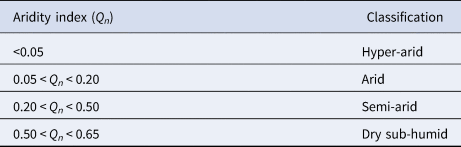
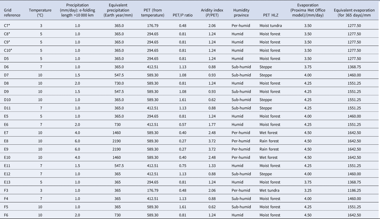
where the aridity index (Q n) is the ratio of annual precipitation, P, to the potential evapotranspiration, PET. Both components are expressed in millimetres. For tidally-locked worlds, with short orbital periods, calculations for the table are extrapolated from 1 to 365 days (the terrestrial year). This provides a means of simple comparison with terrestrial measures. Table 1 indicates the comparative index value with its classification. Table 2 summarizes the output based on these calculations.
Comparison of aridity index values with terrestrial biozones

Daily precipitation rate is divided by PET. Areas with Q n values exceeding 0.65 are not considered arid. Proxima b is largely hyper-arid (polar desert), with rainfall totals less than 1 mm per year.
Holdridge mapping of potential vegetation using an e-folding length for precipitation of 10 000 km

Precipitation
Modelling of precipitation has been performed for aquaplanets (Boutle et al., Reference Boutle, Mayne, Drummond, Manners, Goyal, Lambert, Acreman and Earnshaw2017) but not for planets with varied surface topography. In principle, this could limit the application of climate models to considerations of habitability. However, empirical studies of terrestrial precipitation have uncovered some interesting – and very helpful – relationships.
In areas with abundant vegetation, precipitation remains constant (or even increases) with distance from water sources (oceans, seas and large lakes, Makarieva et al., Reference Makarieva, Gorshkov and Li2009). Areas with sparse vegetation show rapid declines. The distribution of rainfall along storm tracks can be defined by the linear regression:

where P is the precipitation rate, x is the distance from the water source and b is defined by equation (5):

Here, l is the precipitation e-folding length, which assumes values of several hundred kilometres with a terrestrial mean of 600 km. However, the terrestrial average is misleading. Precipitation declines with an e-folding length of 800–900 km across moist, warm temperate regions, with mixed vegetation. For example, l has a value of 830 km across the Eastern seaboard of North America and 860 km across the equivalent region of Eastern China. This value is dwarfed by an e-folding length of 14 000 km for interior North America, with abundant Taiga and mixed forest. Here, there is little decline in precipitation from the Arctic Ocean to the continental interior (Makarieva et al., Reference Makarieva, Gorshkov and Li2009). The same group found no statistically-significant variation in the precipitation rate with distance for the Amazonian and Congo rainforest regions. However, the deep continental river basins of the Ob, Mackenzie, Yenisey and Lena, the e-folding length, l, adopted negative values of −(2, 2, 3 and 4) × 103 km, respectively, indicating modest increases in precipitation, with distance from the Arctic and Atlantic Oceans. Comparison with desertified regions showed a straightforward exponential decrease in precipitation with distance from water sources, with characteristic values of l = ~230–260 km.
Taken together, this indicates that vegetation plays a pivotal role in the preservation and cycling of water on Earth and once present, dominates the effects of moisture transport from distant sources. This agrees with measurements of continental evapotranspiration, which show that 80–90% of terrestrial water flux is through vegetation, not simple evaporation from land surfaces (Jasechko et al., Reference Jasechko, Sharp, Gibson, Birks, Yi and Fawcett2013). These observations allow the direct application of climate models to planets, irrespective of the continental area. On landscapes free of vegetation, the e-folding lengths from terrestrial observations are applicable (with an exponential decline in precipitation with an e-folding length of 230 km). On vegetated surfaces the values for P can be taken directly from the aquaplanet climate models as there is unlikely to be significant variation over long continental stretches.
In summary, the equations outlined above allow us to determine the niche volume of a region, as well as define it in terms of its Holdridge Life-Zone (HLZ) characteristics. The former will be described in a separate paper.
Climate model input and assumptions
A variety of climate models are available for tidally-locked planets with a range of orbital periods (Carone et al., Reference Carone, Keppens and Decin2015; Kopparapu et al., Reference Kopparapu, Wolf, Haqq-Misra, Yang, Kasting, Meadows, Terrien and Mahadeva2016; Haqq-Misra et al., Reference Haqq-Misra, Wolf, Joshi, Zhang and Kopparapu2018). These provide temperature and precipitation, which makes them amenable to further phytoclimatic mapping using the Holdridge criteria. In this paper, we employ the Met Office temperature and precipitation models of Proxima b to produce realistic surface habitability models for Proxima b (Boutle et al., Reference Boutle, Mayne, Drummond, Manners, Goyal, Lambert, Acreman and Earnshaw2017). While we have no idea whether Proxima b has sufficient surface water to support a biosphere, never mind has a biosphere, the output presented in this study demonstrates the suitability of the approach. With relatively few parameters, we can determine the biological potential of exoplanets, irrespective of their host star and orbital parameter.
We should also note that while Holdridge, obviously, only considered the Earth and its vegetation, if we assume that vegetative autotrophs (aka plants) are possible on any world, then the phytoclimatic maps presented here will also delineate the kinds of vegetation possible on different areas of exoplanets. We are, however, making no assumptions about what that vegetation will look like, other than that it will carry out photosynthesis and will transport water via cohesion–tension/transpiration pull. Anything with an active (metabolic) pump for fluids will not be constrained in the same manner. However, on biological grounds, this organism will not be a plant, as it will not be able to support the transport of water through the energy obtained from light via photosynthesis.
It is also worth emphasizing that in choosing Proxima b, we are not making assumptions as to the suitability of red dwarf planets to support biospheres. Proxima b is chosen solely because high-resolution climate data are available, which is then amenable to further analysis (Boutle et al., Reference Boutle, Mayne, Drummond, Manners, Goyal, Lambert, Acreman and Earnshaw2017). The model is applicable to any planet, with sufficient water to support a hydrological cycle. The HLZM has already been successfully applied to the terrestrial biosphere and provides a robust match to observed plant communities (Holdridge, Reference Holdridge1966, other references). Therefore, we assume that the model is directly applicable to asynchronously-rotating planets elsewhere, where sufficient water is present.
Results
Application of Holdridge Life Zones to tidally-locked planets
Two models were used to interpret the biological potential of a wet Proxima b: i.e. one which has not had much of its atmosphere stripped by stellar winds and XEUV (Wheatley et al., Reference Wheatley, Louden, Bourrier, Ehrenreich and Gillon2016; Lingam and Loeb, Reference Lingam and Loeb2018). In the first, the e-folding length is set to greater than 10 000 km and in the second to 250 km. These represent the end-members of the precipitation patterns observed on Earth (Makarieva et al., Reference Makarieva, Gorshkov and Li2009).
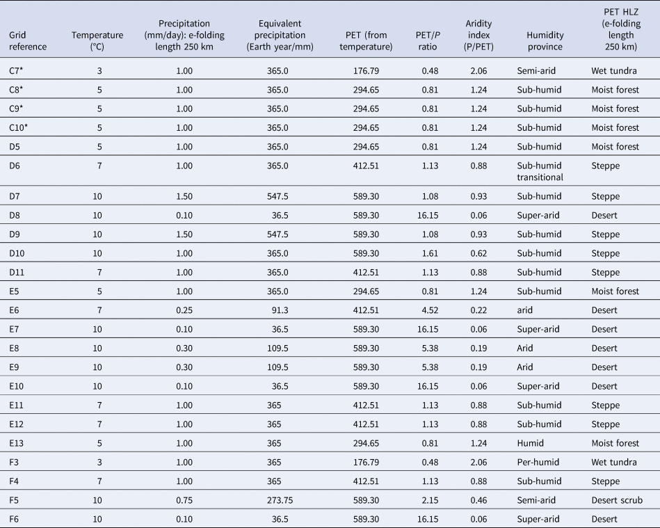
Tables 2 and 3 provide a summary of the HLZM characteristics and input data as it is applied to the habitable regions on the surface of Proxima b. Here, we assume that there is sufficient water available to allow the development of a biosphere. To provide a valid comparison with the original Holdridge criteria, measures of potential evapotranspiration will be determined from temperature alone. However, for comparison, Table 2 provides the evaporation rate (mm/day), averaged for the squares across the model planet. An interesting point is that, for the exception of the areas with the highest temperatures, the Met Office model consistently gives higher rates of evaporation than the potential evapotranspiration rates from Holdridge. However, evapotranspiration requires vegetation and in the Holdridge system, PET is only applicable where the temperature exceeds 4.5–5°C, for the terrestrial biosphere.
Holdridge mapping of potential vegetation using an e-folding length of 250 km

To produce a viable grid output, temperatures are averaged across all of the grid units, except for those highlighted in red, which form the periphery of the region surrounding the sub-stellar point (SSP). Here, the temperatures only exceed the 5°C limit in areas closest to the SSP. The remainder of these blocks is likely to be glaciated (or cold desert), with the model of Bouttle et al. suggesting persistent light snowfall (Boutle et al., Reference Boutle, Mayne, Drummond, Manners, Goyal, Lambert, Acreman and Earnshaw2017). Outside this region, the planet is dry and cold, giving polar desert (hyper-arid) conditions. Freezing fogs may provide some moisture, otherwise any biosphere must be sub-surface if it is to obtain moisture and sufficient warmth to propagate.
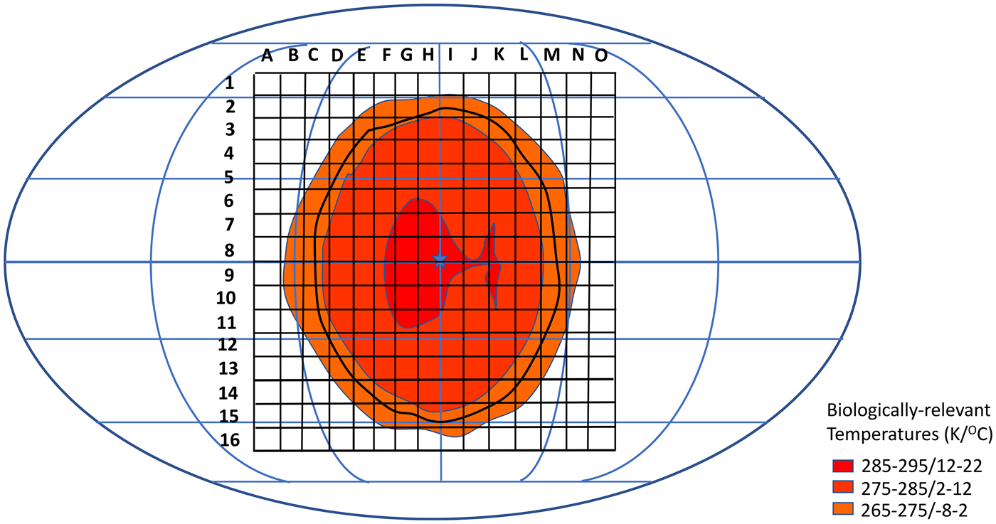
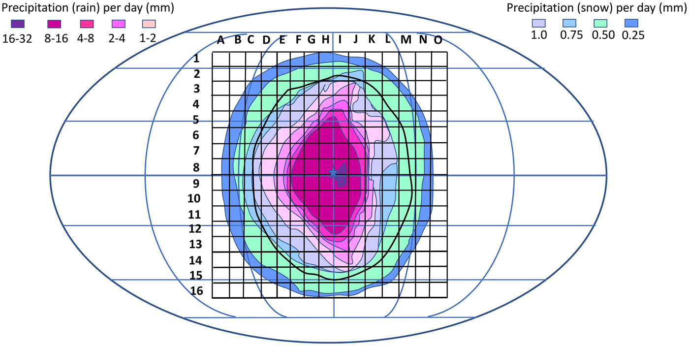
The model output of Bouttle et al. was scaled and gridded to provide averaged temperatures. Each block is ~1300 km wide if we assume that Proxima b has a radius of 1.1-Earths (~7100 km, with a circumference of 45 000 km). Figure 1 shows the grid of biologically-relevant temperatures, while Fig. 2 illustrates the precipitation over the equivalent region.
Simplified Proxima b temperature map from Bouttle et al. Gridding is used to define regions for subsequent analysis. The thick black line marks the edge of our arbitrarily placed supercontinent.

Gridded precipitation plot, adapted from Bouttle et al. This is used in subsequent calculations of the PET/P ratio.

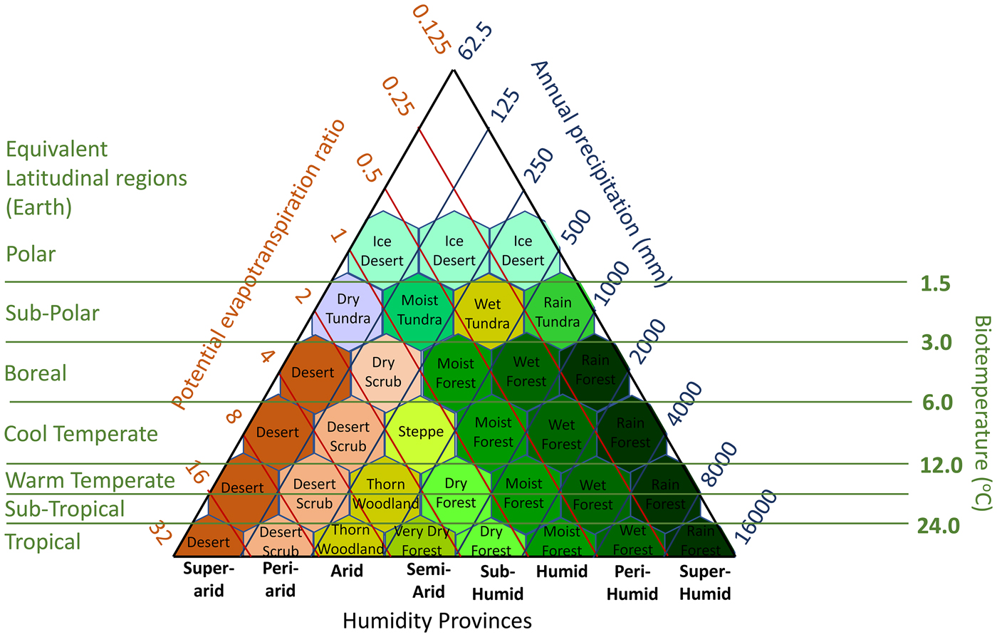
Figure 3 illustrates the HLZs in relation to PET, precipitation and aridity.
HLZs, based on temperature, potential evapotranspiration ratio and precipitation. The system uses very few variables to define the limits to different vegetation regimes on Earth and has shown broad application despite its genesis in tropical ecosystems. Colour coding is the same as used in the subsequent figures.

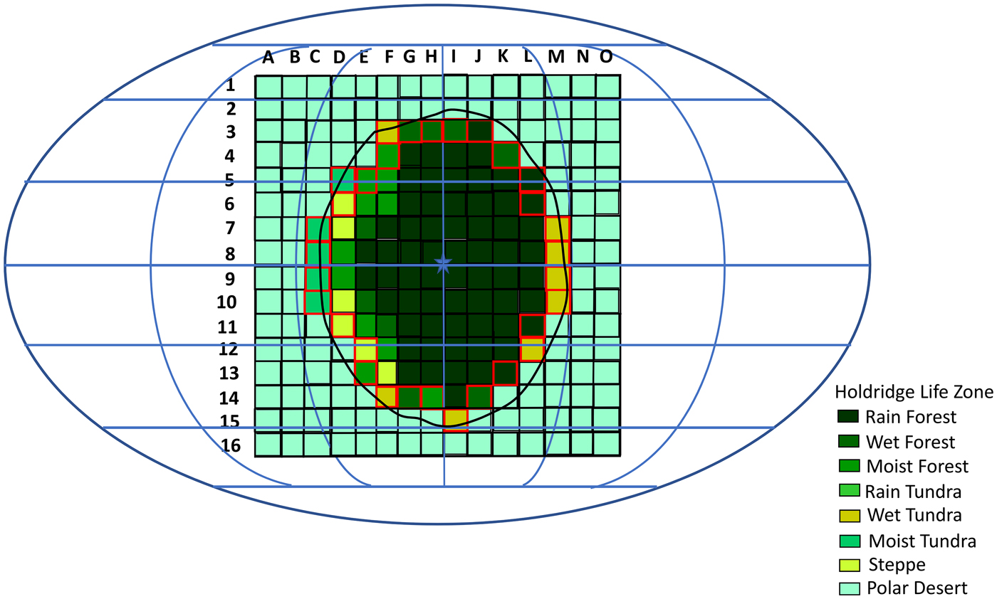
These first-generation models have low resolution, to clearly illustrate the output and also to simplify the analysis. However, the mathematics is straightforward and can be applied to higher resolution gridded data. This would obviously smooth the output and provide a more realistic representation of (potential) biodiversity. However, what these models illustrate is that the principle vegetation types on Proxima b or related, tidally-locked planet, are limited to one area because of tight coupling of temperature and precipitation. This restricts the number of HLZs to a smaller number than found on Earth. Precipitation is primarily expected to be convectional and restricted to the region closest to the SSP. Peripheral regions may have precipitation (perhaps orographic), but these have temperatures that are insufficient for plant growth. Figure 4 illustrates the output in Table 2 in a qualitative manner.
HLZ application to Proxima b with on a hypothetical land surface covering the region where life is possible. We assume that there is sufficient moisture available to supply the land surface through inflowing winds according to Bouttle et al. In this mode, the e-folding length is set to greater than 10 000 km (approximately ten squares) in accordance with terrestrial observations for continental surfaces and precipitation. Despite some decrease in moisture towards the interior, a rain-forest climate is possible. Red peripheral squares have marginal temperatures over much of their surface, limiting the potential for vegetation.

Most of the planets that do have suitable temperatures and rainfall have conditions amenable to the growth of forests. There is a strip around this region that could host either steppe (cool, temperate) conditions or tundra-like biomes. In total, the area that is habitable for complex life is limited to a radius of 7700 km around the SSP, in a roughly circular area of ~186 million km2. The terrestrial surface (that not covered in water) has an area of 131 646 971 km2. While this might imply that Proxima b has a larger habitable land surface, this neglects any realistic distribution of land masses. Obviously, while it is possible that the entire area surrounding the SSP is land, it would be more realistic if the land was distributed in a less favourable arrangement. Therefore, one should always expect that the area of land that is habitable for complex life will be less on synchronously-rotating worlds than those that have asynchronous rotation. This gives a quantitative assessment of the habitability in relation to addressing the Fermi Paradox (Stevenson, Reference Zeng, Sasselov and Jacobsen2018b). With less habitable surface on which complex life can evolve and fill niches, the evolutionary complexity of life on these worlds will always be lower than that it is on asynchronously-rotating planets.
In terms of the kind of forest, conditions are broadly similar to temperate rainforest: 7–22°C; with rainfall varying from 1000 to 5000 mm per annum in the model which has an e-folding length of greater than 10 000 km (Fig. 4).
Continentality
In the first model (Fig. 4), the e-folding length, the distance over which rainfall declines by 50% of the initial value, was set to greater than 10 000 km. Given the dimensions of our super-continent, this expression allows precipitation to follow the Met Office model and allows the landscape to become fully vegetated, if sufficient water was available from external sources (Makarieva et al., Reference Makarieva, Gorshkov and Li2009). Rainfall does not decline with distance to the centre of the region of interest, but follows an increase set by the Met Office model (Boutle et al., Reference Boutle, Mayne, Drummond, Manners, Goyal, Lambert, Acreman and Earnshaw2017). A more modest interpretation, with a flat distribution of rainfall (or one showing a slight increase towards the interior) still produces either wet forest or rain forest across most of the surface. Here, precipitation is held at 1000 mm per Earth-year equivalent (figure, not shown). In both instances, moisture must be recycled efficiently over the interior (van der Ent et al., Reference van der Ent, Savenije, Schaefli and Steele-Dunne2010). This assumes that vegetation is present and will be able to pump significant quantities of moisture back to the atmosphere that precipitate onto the surface (Peel et al., Reference Peel, McMahon and Finlayson2010; Jasechko et al., Reference Jasechko, Sharp, Gibson, Birks, Yi and Fawcett2013; Stan et al., Reference Stan, Neculau, Liliana Zaharia and Ioana-Toroimac2014). Poorly-vegetated surfaces have lower evapotranspiration rates than assumed in Holdridge.
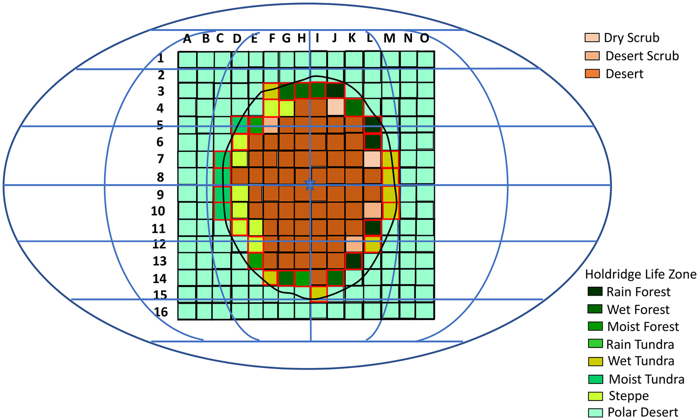
To illustrate this concept, we apply a second model (Fig. 5), where the e-folding length is set to 250 km. This is more applicable to landscapes that are not vegetated on some continental margins on Earth (Makarieva et al., Reference Makarieva, Gorshkov and Li2009). Obviously, rainfall is limited to the peripheral margins of the continental region and the majority of the interior is desert. While precipitation is limited to the periphery, the surface still has a substantial region over which precipitation could support a variety of vegetation types. Again, temperature becomes the limiting factor for plant growth in this model. This is more important in the second model, because areas with sufficient precipitation have temperatures that are marginal for photosynthesis.
The same model as Fig. 4, but with the e-folding length reduced to 250 km (approximately one-quarter square), in accordance with terrestrial observations of some non-vegetated margins. Rainfall decreases promptly across peripheral squares. Therefore, vegetation illustrated is the maximum possible, but likely confined to the outermost 500 km of each square. Interior squares have minimal precipitation. Red peripheral squares have marginal temperatures (2–5°C), limiting the actual area where plant life would be possible.

One must also remember that for the purposes of this paper, the area that has precipitation is assumed to be land, rather than ocean, but flanked on ocean on all sides. In practice, this is unlikely to be true, unless a supercontinent is anchored by some means under the SSP.
Succession and topography
While we are not going to formally address succession, colonization of new surfaces will adapt the surface to match the surrounding landscape in a manner dependent on its altitude. Landscapes at the sea level will populate with the vegetation type illustrated in Figs. 4 or 5. HLZs are also available for biomes at varying altitudes (Holdridge, Reference Holdridge1966, Fig. 3). While we do not consider these in detail here, in general we assume a decrease in temperature of 5–6°C every 300 m or so in dry air and 3°C per 300 m for air that is saturated. The outermost grid cells (those edged in red) will become uninhabitable for plants at only modest altitudes, with the snow line rising from the sea level along the distal edges of the outermost cells to a little over 2400 m near the SSP. We assume that air is fully saturated in all of the grid cells in this estimation. If the air is significantly drier, then the snow line will be correspondingly lower.
One consequence of succession is the change in precipitation over geological timescales. With transpiration rates greatly exceeding evaporation rates at any given temperature, when land is colonized by vegetation as a consequence of evolutionary succession (rather than primary succession) changes in moisture recycling to the local atmosphere, will facilitate the spread of vegetation over all available land. This will lead to the progressive colonization of all land from coastal areas towards the interior as regional humidity levels increase, cloud levels rise and precipitation increases. The radial inflow of air towards the SSP would clearly facilitate this spread towards the interior.
On asynchronously rotating planets, migration of precipitation and vegetation towards the continental interior will follow the regional pattern of airflow, dictated by the relative strength of the Coriolis effect and thermal gradient.
Topography aligned at a steep angle to the prevailing wind, such as the Rockies in relation to the mid-latitudinal westerlies, will create local or regional rain-shadows. The effect varies with the kind of airflow that impacts the windward slope (Siler et al., Reference Siler, Roe and Durran2012). For planets with hemispheric Hadley cells (all synchronously-rotating planets with periods greater than 5 days), radial inflow of air towards the SSP may generate regional rain shadows. However, the effect on continental scales is surprisingly slight with very limited impact on phytoclimatic distribution of species, except where the mountains are particularly high (Botti, Reference Botti2018). However, Kukla et al. use oxygen isotopes to illustrate the effect of significant barriers on the recycling of moisture (Kukla et al., Reference Kukla, Winnick, Maher, Ibarra and Chamberlain2019). These show significant changes in moisture transport across mountain barriers, in a manner consistent with the height and continuity of the barrier. However, while we expect such obstacles to influence moisture transport on real planetary surfaces, quantifying these is beyond the reach of this paper. Comparison of O18 isotopes in terrestrial settings will provide the way forward, in this regard.
Application to asynchronously-rotating planets
Here, the models should follow the terrestrial pattern, with precipitation greatest in equatorial regions and along windward coasts affected by westerly storm tracks. However, transects were not pursued along West–East paths in Makarieva, Gorshkov and Li's research (Makarieva et al., Reference Makarieva, Gorshkov and Li2009), therefore, we need to be a little careful. Examination of the phytoclimatic maps of Europe (Defaut, Reference Defaut1991; Botti, Reference Botti2018) provides some useful empirical data. Aridity as measured by equation (1), broadly follows latitudinal banding, with dry conditions in the south, grading into wetter conditions as we move northwards. This offsets ‘continentality’, where strong seasonal variations in temperature have limited impact on the aridity of the landscape. This implies that the precipitation pattern on asynchronously-rotating planets should, broadly, follow that of the other margins modelled in Makarieva et al., (Reference Makarieva, Gorshkov and Li2009).
Discussion
This paper represents a first attempt to mathematically constrain and model the biological potential of exoplanets. While, we cannot predict the precise evolutionary pathway of any given planet, the fundamental laws that dictate processes, such as evolution through natural selection, or the transport of water in biological systems, are constrained by the underlying physics. In this regard, this paper presents realistic first-generation models that explore the ecological systems that are permitted by climate models. In this regard, the models are applicable to a wide range of planets, irrespective of their host star, orbital parameter or the presence or absence of tidal-locking.
Crucially, the models delineate the kinds of living forms that are possible, using a limited number of climate parameters that are available from a number of studies. Thus, the beauty of these models lies in the simplicity of the underlying science. Importantly, the model assumptions have been extensively validated by a number of terrestrial studies (Holdridge, Reference Holdridge1966; MacMahon and Wieboldt, Reference MacMahon and Wieboldt1978; Yates et al., Reference Yates, Kittel and Cannon2000; Nasir et al., Reference Nasir, Afrasiyab and Athar2015; Tekin et al., Reference Tekin, Tatlh and Koç2018). While there are clear limitations to their application, over regional scales and in diverse environments, the HLZM holds considerable validity. As a first generation run, the climate output from the Proxima b models was gridded and the data used to constrain the possible life zones as defined using the method of Holdridge (Holdridge, Reference Holdridge1966). Subsequent work will be carried out with higher resolution climate data. However, in this instance the resolution of the climate data is sufficient to produce a realistic output.
Some assumptions are made regarding moisture fluxes towards the interior of the continent. Firstly, that there is sufficient moisture blowing inwards towards the SSP. One may question this if the surrounding surface is frozen. However, here, the principle is merely to show what will happen if the moisture is available; not whether the climate model of Bouttle et al. is able to do so.
Secondly, from this starting assumption, to provide a realistic model, sensible ranges of moisture recycling are applied. From empirical measurements, we can determine the efficiency of moisture transportation to the interior of land-masses. Two extreme end-members are used in this study: one where precipitation declines with an e-folding length of 250 km and a second where the value exceeds 10 000 km. In each, the HLZM provides sensible outputs that can be related to terrestrial observations. In practice, the difference in the two model parameters may be due to differences in moisture recycling by terrestrial vegetation; or be down to differences in atmospheric circulation patterns in the terrestrial systems over the regions that Makarieva et al. consider. If the differences in the e-folding lengths are attributable to variation in moisture recycling by vegetation, one should consider the impact of evolutionary succession. In poorly-vegetated areas, moisture recycling may be low, but this will increase over time as vegetation colonizes areas. This may be over decadal timescales, in the case of standard primary succession, or on geological timescales as species evolve to fill the available niches.
Fully, 80–90% of terrestrial water flux is through plants rather than conventional evaporation. Therefore, we should always expect vegetation-free landscapes that are distant from moisture sources to be drier than those that have vegetation (Peel et al., Reference Peel, McMahon and Finlayson2010; Jasechko et al., Reference Jasechko, Sharp, Gibson, Birks, Yi and Fawcett2013; Stan et al., Reference Stan, Neculau, Liliana Zaharia and Ioana-Toroimac2014).
In conclusion, this work provides a realistic framework to consider planetary habitability using a relatively small number of definable quantities, making it a valid and highly applicable basis for further consideration of habitability and evolutionary potential.
Supplementary material
The supplementary material for this article can be found at https://doi.org/10.1017/S1473550419000181.
Acknowledgement
The author would like to thank the anonymous reviewer who made some helpful suggestions, which have improved the structure and accessibility of this article.