1. Introduction
The general turbulence problem is of course far from solved, whether in terms of mathematical and intuitive understanding, or in terms of obtaining a certain accuracy that depends on viscous fluid dynamics. However, turbulent flow is of interest to turbulence researchers because of its wide range of occurrence across many engineering disciplines; thus large amounts of ongoing research are devoted to a better understanding of the complex mechanisms of turbulence.
The whole range of spatial and temporal scales of turbulence can be resolved through a direct numerical simulation (DNS) of the Navier–Stokes equations. However DNS is not possible for all turbulent flow cases because its computational cost makes it infeasible; for this reason, it is only applied to very simple geometrical configurations, such as channel flow, and moderate Reynolds numbers. For more complex situations, Reynolds-averaged Navier–Stokes (RANS) equations, derived, as the name implies, from a statistical averaging of the Navier–Stokes equations, are adopted. One of the main difficulties in the use of this set of equations is represented by the closure problem, that is the addition of empirical (algebraic or differential) relationships to model the Reynolds stresses. Already the fact that a certain number of models are in common use shows that the modelling of these terms can hardly be given a universal form valid for all cases.
The capability of RANS models to predict the behaviour of channel flow has been investigated by a number of researchers, using both numerical and experimental techniques. Patel, Rodi & Scheuerer (Reference Patel, Rodi and Scheuerer1985) considered eight two-equation, ‘low-Reynolds-number’ turbulence models and compared their results with available experimental data. Myong & Kasagi (Reference Myong and Kasagi1990) proposed an improved near-wall
 $k$
–
 ${\it\epsilon}$
turbulence model considering the two characteristic length scales for the dissipation rate, one very near the wall and the other remote from the wall, which were then related to the length scale of turbulent momentum transfer. Several near-wall two-equation models were compared with data obtained from direct numerical simulations at very low Reynolds numbers by Sarkar & So (Reference Sarkar and So1997).
In the present paper a benchmark problem is proposed, simple enough that it can be solved both by an eddy-viscosity model and by DNS: this is the linear response of a turbulent flow’s mean-velocity profile to a steady volume force. Luchini & Charru (Reference Luchini and Charru2010a ,Reference Luchini and Charru b ), while studying the phase lead of shear stress at a channel’s perturbed bottom, provided consistent corrections to the bottom shear stress and pressure gradient arising from slow changes in the water depth. They carried out the analysis of both laminar and turbulent flow in two different ways: a straightforward perturbative expansion of the velocity profile and a consistent section-averaged equation. In particular, under turbulent-flow conditions, RANS equations were closed with a variable eddy viscosity. This model is similar to those typically used in shallow-water flow calculations and derived through consistency with the unperturbed flow (see Jackson & Hunt Reference Jackson and Hunt1975; Jimenez et al. Reference Jimenez, Uhlmann, Pinelli and Kawahara2001). The application of a perturbative expansion to this set of equations to simulate the effect of a slowly variable geometry produced something similar to a forcing term which is only a function of the wall-normal coordinate. The straight-channel flow with a forcing term, however, is a meaningful physical problem in itself, which can be solved independently of its appearance in the context of bottom wall modulations.
Therefore, in this paper a channel flow subject to an external volume force, at moderate but turbulent Reynolds number, will be considered. The DNS solution of this problem will be compared to the corresponding RANS solution closed with the algebraic turbulence model considered by Luchini & Charru (Reference Luchini and Charru2010a ). Since the domain is very simple and the Reynolds number is small, the same problem can be solved in both ways, and the results of a DNS can be compared with those obtained with the above mentioned turbulence model. In particular we shall study the linear response of turbulent flow, the one that can be observed when the amplitude of the applied perturbation is small enough, even though a turbulent flow is a nonlinear system. To do this we shall adapt the method by which Quadrio & Luchini (Reference Quadrio and Luchini2002) and Luchini, Quadrio & Zuccher (Reference Luchini, Quadrio and Zuccher2006) computed the average linear impulse response of a wall-bounded turbulent flow as a function of spatial and temporal separations. In those papers the characterization in the frequency domain is obtained in terms of the response of the system to sinusoidal forcing of varying frequency, or in the time domain as the response to a Dirac function, the former being the Fourier transform of the latter, and the response of the system is written as a convolution integral of the transfer function and the forcing input. Our present case will be actually simpler, since we are only concerned with the steady, zero-frequency, component.
This paper is organized as follows. The benchmark problem will be illustrated in § 2. The laminar solution of the benchmark problem is described in § 3. The eddy-viscosity model and the mean linear response of turbulent flow to a volume force will be discussed in § 4 with the analysis of the results in the constant-flow-rate and constant-pressure-gradient case. The conclusions will be discussed in § 5. Appendix A describes how the linear response to an external volume force is related to Luchini & Charru (Reference Luchini and Charru2010a ,Reference Luchini and Charru b )’s problem of flow past an undulated wall.
2. Flow in a plane channel under an external volume force
The benchmark problem is the calculation of the linear response of turbulent flow to an external volume force in an infinite plane channel. This flow is governed by the Navier–Stokes equations, with the addition of an infinitesimal external volume force
 $\boldsymbol{F}^{\prime }=[{\it\epsilon}F(y),0,0]$
directed in the streamwise direction which is a function of
 $y$
only. The appropriate boundary conditions impose zero velocity at the walls and periodicity in the two homogeneous directions. If the streamwise, wall-normal and spanwise coordinates are respectively x, y and z and
 $\boldsymbol{u}=[u,v,w]$
represents the non-dimensional velocity vector, the incompressible Navier–Stokes (NS) equations can be written as
 $$\begin{eqnarray}\left.\begin{array}{@{}c@{}}\boldsymbol{{\rm\nabla}}\boldsymbol{\cdot }\boldsymbol{u}=0,\\ \displaystyle \frac{\partial \boldsymbol{u}}{\partial t}+\boldsymbol{u}\boldsymbol{\cdot }\boldsymbol{{\rm\nabla}}\boldsymbol{u}=-\boldsymbol{{\rm\nabla}}p+\frac{1}{Re}{\rm\nabla}^{2}\boldsymbol{u}+\boldsymbol{F}^{\prime },\end{array}\right\}\end{eqnarray}$$
where the Reynolds number is based on the half height of the channel and the bulk velocity; in other words the dimensionless height of the channel is
 $2$
.
 ${\it\epsilon}$
is a small constant, finite for numerical purposes but small enough for the limit
 ${\it\epsilon}\rightarrow 0$
to be approached. The boundary conditions at the two walls for the three components of velocity are
 $u=v=w=0$
. The mean flow can be generated in two different ways, by imposing a constant-in-time streamwise pressure gradient (CPG) or a constant-in-time flow rate (CFR); both possibilities will be considered.
The main difference between the two cases is that, in the CPG configurations, wall shear stress after the perturbation remains the same as before (Quadrio & Ricco Reference Quadrio and Ricco2011), unlike what happens in the CFR situations (see Hœpffner & Fukagata Reference Hœpffner and Fukagata2009; Kasagi, Hasegawa & Fukagata Reference Kasagi, Hasegawa and Fukagata2009). Instead of CPG or CFR configurations, a novel approach based on the constant power has been proposed in Frohnapfel, Hasegawa & Quadrio (Reference Frohnapfel, Hasegawa and Quadrio2012) and Hasegawa, Quadrio & Frohnapfel (Reference Hasegawa, Quadrio and Frohnapfel2014).
Four volume-force profiles will be considered:
 $$\begin{eqnarray}\displaystyle (1)\quad F(y) & \hspace{-2.0pt}=\hspace{-2.0pt} & \displaystyle U^{2}(y)-\{U^{2}(y)\},\end{eqnarray}$$
 $$\begin{eqnarray}\displaystyle (2)\quad F(y) & \hspace{-2.0pt}=\hspace{-2.0pt} & \displaystyle -\!\cos ({\rm\pi}y),\end{eqnarray}$$
 $$\begin{eqnarray}\displaystyle (3)\quad F(y) & \hspace{-2.0pt}=\hspace{-2.0pt} & \displaystyle \sin (2{\rm\pi}y),\end{eqnarray}$$
 $$\begin{eqnarray}\displaystyle (4)\quad F(y) & \hspace{-2.0pt}=\hspace{-2.0pt} & \displaystyle \cos (2{\rm\pi}y).\end{eqnarray}$$
 $x$
,
 $z$
and time-mean values are indicated with angular brackets, so
 $U=\langle u\rangle$
, while
 $\{U^{2}\}$
is the mean value in the
 $y$
direction of
 $U^{2}(y)$
.) Sinusoidal symmetric and anti-symmetric forces will be considered insofar as representative of a generic force profile expanded in a Fourier series.
The forcing-term coefficient
 ${\it\epsilon}$
is chosen small enough to have a linear response of the system, but sufficiently large for the response of velocity to be distinguished from the statistical fluctuations typical of turbulent flow. For small
 ${\it\epsilon}$
, a perturbation expansion of the solution can be written as
 $$\begin{eqnarray}U_{1}\simeq U_{0}+{\it\epsilon}{\it\delta}U+o({\it\epsilon}^{2}),\end{eqnarray}$$
where
 $U_{0}(y)$
is the
 $x$
,
 $z$
and time-averaged streamwise velocity when no forcing is applied,
 $U_{1}(y)$
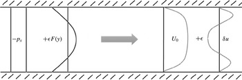
denotes the solution in the perturbed case (see figure 1) and
 ${\it\delta}U(y)$
is the sought-for linear response.
Sketch of the linear response of streamwise velocity to the forcing term (2.3).

All the volume forces in (2.2) are characterized by a
 $y$
-integral calculated on the half height of the channel equal to zero; in fact, the constant part of any possible applied forcing can always be included in the streamwise pressure gradient
 $p_{x}$
. Moreover, let’s consider the averaged streamwise component of the momentum equation in the case of parallel flow (i.e. when the streamwise and the spanwise derivatives are equal to zero)
 $$\begin{eqnarray}0=\frac{\text{d}{\it\tau}}{\text{d}y}-\langle p_{x}\rangle +{\it\epsilon}F(y).\end{eqnarray}$$
The total shear stress
 ${\it\tau}(y)$
is equal to
 $$\begin{eqnarray}{\it\tau}=\frac{1}{Re}\frac{\text{d}\langle u\rangle }{\text{d}y}-\langle u^{\prime }v^{\prime }\rangle ,\end{eqnarray}$$
where
 $u^{\prime }$
and
 $v^{\prime }$
are respectively the streamwise and wall-normal components of the fluctuation velocity vector
 $\boldsymbol{u}^{\prime }=[u^{\prime },v^{\prime },w^{\prime }]$
and
 $\langle u^{\prime }v^{\prime }\rangle$
is one component of the Reynolds stresses. The integral form of (2.4) implies
 $$\begin{eqnarray}{\it\tau}_{w}=-P_{x}+{\it\epsilon}\int _{0}^{1}F(y)\,\text{d}y,\end{eqnarray}$$
where
 ${\it\tau}_{w}=Re^{-1}(\text{d}U/\text{d}y)_{y=0}$
and
 $\langle p_{x}\rangle =P_{x}$
. Equation (2.6) shows that if the force has zero integral the equality between pressure gradient and wall shear stress remains unaffected.
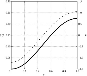
Laminar solution:
 ${\it\delta}U$
——,
 $F$
– – –.

3. Laminar solution
In preparation for the subsequent analysis of turbulent flow, let us start by examining the laminar solution to the problem (2.1). Let us consider the particular case of the volume force relevant to Luchini & Charru (Reference Luchini and Charru2010b ) defined by (2.2a ). In the case of laminar flow, the forcing term (2.2a ) will have the following analytical expression:
 $$\begin{eqnarray}F(y)=U^{2}(y)-\{U^{2}(y)\}=\left(3y-{\textstyle \frac{3}{2}}y^{2}\right)^{2}-{\textstyle \frac{6}{5}}.\end{eqnarray}$$
The laminar mean flow in a plane channel is governed by the Poiseuille solution of (2.1), in which all the nonlinear terms are zero even in presence of a volume force. The Navier–Stokes momentum equation thus simplifies to
 $$\begin{eqnarray}\frac{U_{yy}}{Re}=-P_{x}+{\it\epsilon}F.\end{eqnarray}$$
Since this equation is linear, the streamwise velocity perturbation (
 ${\it\delta}U$
) obeys a similar equation
 $$\begin{eqnarray}\frac{{\it\delta}U_{yy}}{Re}=-{\it\delta}P_{x}+F.\end{eqnarray}$$
In the case of constant pressure gradient,
 ${\it\delta}P_{x}$
is equal to zero. Two boundary conditions are imposed (i.e.
 ${\it\delta}U(y=0)={\it\delta}U(y=2)=0$
), so the solution of (3.3) is
 $$\begin{eqnarray}{\it\delta}U=Re\int _{0}^{y}\left(\int _{0}^{y}F\,\text{d}y\right)\text{d}y.\end{eqnarray}$$
By substituting formula (2.2a
) into (3.4), the expression of
 ${\it\delta}U$
turns out to be
 $$\begin{eqnarray}{\it\delta}U=Re\frac{24y^{2}-30y^{4}+18y^{5}-3y^{6}}{40}.\end{eqnarray}$$
Figure 2 shows that
 ${\it\delta}U$
is everywhere positive and monotonic, despite the volume force being negative in the portion of the channel closest to the wall and has a
 $y$
-integral equal to zero. It follows that a flow rate increase is generated without any resultant applied force or any reaction on the wall. (A similar phenomenon occurs in steady streaming, see Luchini (Reference Luchini2008).) Although at first puzzling, this behaviour is evident from the analytical solution of the problem.
Physically, it is not a priori predictable whether the application of an external volume force with zero
 $y$
-integral will give a positive or a negative contribution to flow rate, because the forcing term is pushing the flow in one direction in a part of the channel and in the opposite direction in the other part. However, from the analytical solution (see (3.5)) of problem (3.3), in laminar flow, it is clear that the calculated flow rate perturbation is positive.
4. Turbulent flow
This section is devoted to the linear response of turbulent flow to an external volume force. This problem is simple enough that it can be solved both by a turbulence model and by DNS. Here we consider an algebraic eddy-viscosity model that is consistent with the mean flow. The mean linear response of several quantities, in particular streamwise velocity, pressure gradient and flow rate, will be compared with those obtained from DNS.
4.1. Eddy-viscosity model
Let’s consider the non-dimensional form of the Reynolds-averaged Navier–Stokes equations (as reported by Pope (Reference Pope2011))
 $$\begin{eqnarray}\boldsymbol{{\rm\nabla}}\boldsymbol{\cdot }(\langle \boldsymbol{u}\boldsymbol{u}\rangle )=-\boldsymbol{{\rm\nabla}}\langle p\rangle +\frac{1}{Re}{\rm\nabla}^{2}\langle \boldsymbol{u}\rangle +\boldsymbol{F}^{\prime }-\boldsymbol{{\rm\nabla}}\boldsymbol{\cdot }(\langle \boldsymbol{u}^{\prime }\boldsymbol{u}^{\prime }\rangle ),\end{eqnarray}$$
where
 $\boldsymbol{u}^{\prime }=[u^{\prime },v^{\prime },w^{\prime }]$
is the fluctuation velocity vector. According to the turbulent-viscosity hypothesis, (4.1) becomes
 $$\begin{eqnarray}\boldsymbol{{\rm\nabla}}\boldsymbol{\cdot }(\langle \boldsymbol{u}\boldsymbol{u}\rangle )=-\boldsymbol{{\rm\nabla}}\left(\langle p\rangle +{\textstyle \frac{2}{3}}k\right)+\boldsymbol{F}^{\prime }-\boldsymbol{{\rm\nabla}}\boldsymbol{\cdot }({\it\nu}_{e}\boldsymbol{{\rm\nabla}}\langle \boldsymbol{u}\rangle ),\end{eqnarray}$$
where
 ${\it\nu}_{e}={\it\nu}_{T}+1/Re$
is the effective viscosity and
 ${\it\nu}_{T}$
represents the eddy viscosity. The closure of these equations, however, require a turbulence model for
 ${\it\nu}_{T}$
and, thus for the shear stress,
 ${\it\tau}$
.
There are several turbulence models from the simpler algebraic viscosity model through the turbulent-kinetic-energy models to the two-equation models (such as
 $k$
–
 ${\it\epsilon}$
models) or the Reynolds-stress-based models (see Wilcox Reference Wilcox1993). The first models are the simplest and easiest to use because they do not involve the resolution of other equations in addition to (4.2) (and they are usually applied in cases of channel or free-shear flows). The more sophisticated models (
 $k$
–
 ${\it\epsilon}$
,
 $k$
–
 ${\it\omega}$
or the Reynolds-stress-based models) are characterized by greater complexity but also an increase of the level of description. Each of these models is characterized by its own expression for the eddy viscosity as a function of some physical quantities (such as
 $k$
,
 ${\it\omega}$
, and so on) which are modelled with additional equations.
According to the
 $k$
–
 ${\it\epsilon}$
model, two model transport equations for the auxiliary quantities turbulent kinetic energy (
 $k$
) and dissipation (
 ${\it\epsilon}$
) are coupled with the RANS equations, i.e.
 $$\begin{eqnarray}\displaystyle & \displaystyle \langle \boldsymbol{u}\rangle \boldsymbol{\cdot }\boldsymbol{{\rm\nabla}}{\it\epsilon}=\boldsymbol{{\rm\nabla}}\boldsymbol{\cdot }\left(\frac{{\it\nu}_{T}}{{\it\sigma}_{{\it\epsilon}}}\boldsymbol{{\rm\nabla}}{\it\epsilon}\right)+C_{{\it\epsilon}1}\frac{{\wp}{\it\epsilon}}{k}-C_{{\it\epsilon}2}\frac{{\it\epsilon}^{2}}{k}, & \displaystyle\end{eqnarray}$$
 $$\begin{eqnarray}\displaystyle & \displaystyle \langle \boldsymbol{u}\rangle \boldsymbol{\cdot }\boldsymbol{{\rm\nabla}}k=\boldsymbol{{\rm\nabla}}\boldsymbol{\cdot }\left(\frac{{\it\nu}_{T}}{{\it\sigma}_{k}}\boldsymbol{{\rm\nabla}}k\right)+{\wp}-{\it\epsilon}, & \displaystyle\end{eqnarray}$$
where
 ${\wp}$
is the rate of production of turbulent kinetic energy and it is defined by equation (5.133) in Pope (Reference Pope2011). In (4.3) and (4.4), the eddy viscosity has the following expression
 $$\begin{eqnarray}{\it\nu}_{T}(y)=c_{{\it\mu}}\frac{k^{2}}{{\it\epsilon}},\end{eqnarray}$$
where
 $c_{{\it\mu}}$
,
 $C_{{\it\epsilon}1}$
and
 $C_{{\it\epsilon}2}$
are adjustable constants that can be derived from data fitting for a wide range of turbulent flows. Pope (Reference Pope2011), in the case of fully turbulent channel flow we simplify the auxiliary equations for
 $k$
and
 ${\it\epsilon}$
to
 $$\begin{eqnarray}\displaystyle & \displaystyle 0=\frac{\text{d}}{\text{d}y}\left(\frac{{\it\nu}_{T}}{{\it\sigma}_{{\it\epsilon}}}\boldsymbol{{\rm\nabla}}\frac{\text{d}{\it\epsilon}}{\text{d}y}\right)+C_{{\it\epsilon}1}\frac{{\wp}{\it\epsilon}}{k}-C_{{\it\epsilon}2}\frac{{\it\epsilon}^{2}}{k}, & \displaystyle\end{eqnarray}$$
 $$\begin{eqnarray}\displaystyle & \displaystyle 0=\frac{\text{d}}{\text{d}y}\left(\frac{{\it\nu}_{T}}{{\it\sigma}_{k}}\frac{\text{d}k}{\text{d}y}\right)+{\wp}-{\it\epsilon}; & \displaystyle\end{eqnarray}$$
so the eddy viscosity defined by (4.5) reduces to a
 $y$
-dependent function and the same happens for other turbulence models.
Following Reynolds & Hussain (Reference Reynolds and Hussain1972), it is also possible to consider the well-known Cess (see Cess Reference Cess1958) analytical approximation for the turbulent eddy viscosity
 $$\begin{eqnarray}{\it\nu}_{e}(y)=\frac{1}{2}+\frac{1}{2}\left[1+\frac{B^{2}Re_{{\it\tau}}}{9}(2y-y^{2})(e-4y+y^{2})^{2}\left[1-\exp \left(\frac{-{\it\eta}Re_{{\it\tau}}}{A}\right)\right]^{2}\right]^{1/2}.\end{eqnarray}$$
The two parameters (
 $A$
and
 $B$
) are derived from a least-square fitting of the mean profile obtained from DNS channel results (see del Alamo & Jimenez Reference del Alamo and Jimenez2006; Hoyas & Jimenez Reference Hoyas and Jimenez2006).
Instead of considering a best fitting of the mean velocity, we decide to use an algebraic eddy-viscosity model (EVM) that is consistent with the unperturbed velocity profile and it is the same as that of Luchini & Charru (Reference Luchini and Charru2010b ) i.e.
 $$\begin{eqnarray}{\it\nu}_{e}(y)=\frac{{\it\tau}_{w}\,(1-y)}{U_{y}},\end{eqnarray}$$
where
 $U_{y}$
is the
 $y$
-derivative of space and time-averaged streamwise velocity and it is obtained from DNS profiles of
 $U$
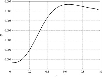
for each Reynolds number. Figure 3 shows the profile of the eddy viscosity versus the wall-normal coordinate, with
 $U$
obtained from DNS data at
 $Re=1700$
. Equation (4.9) was repeatedly used in the past to deduce a turbulent-viscosity diagram from analytical (see Hinze Reference Hinze1975), experimental (see Nezu & Rodi Reference Nezu and Rodi1986) or numerical (see Jimenez et al.
Reference Jimenez, Uhlmann, Pinelli and Kawahara2001) mean-flow velocity profiles because it seems to be the least biased choice.
Eddy-viscosity profile versus the wall-normal coordinate (
 $Re=1700$
).

Since (2.4) is linear, the streamwise velocity perturbation obeys a similar relationship:
 $$\begin{eqnarray}({\it\nu}_{e}(y){\it\delta}U_{y})_{y}=-{\it\delta}P_{x}+F.\end{eqnarray}$$
The approach taken by Jackson & Hunt (Reference Jackson and Hunt1975) is also in the same general class but has an additional factor of two in their equivalent of (4.9) because of the assumed quadratic dependence of stress on velocity. It will be seen that with or without this factor our conclusions are not significantly affected.
Solving (4.10) with the following boundary conditions
 $$\begin{eqnarray}\left.\begin{array}{@{}rcl@{}}{\it\delta}U(0)\,\, & =\,\, & 0,\\ {\it\delta}U_{y}(1)\,\, & =\,\, & 0,\end{array}\right\}\end{eqnarray}$$
gives
 $$\begin{eqnarray}{\it\delta}U_{EVM}=\int _{0}^{y}{\it\nu}_{e}^{-1}\left(\int _{0}^{y}(-{\it\delta}P_{x}+F)\,\text{d}y\right)\text{d}y.\end{eqnarray}$$
In the case of constant pressure gradient,
 ${\it\delta}P_{x}$
is equal to zero.
4.2. Direct numerical simulation of forced flow in a plane channel
This section presents a DNS of channel flow in the presence of volume forcing. The numerical simulations are carried out by Luchini and Quadrio’s DNS pseudospectal solver, the features of which are described elsewhere (Quadrio & Luchini Reference Quadrio and Luchini2006). The computational domain is a periodic box in the
 $x$
and
 $z$
directions. Its dimensions are
 $4{\rm\pi}\times 2{\rm\pi}\times 2$
respectively in the
 $x$
,
 $z$
and
 $y$
directions. The discretization is based on Fourier expansion in the homogeneous directions
 $x$
and
 $z$
and a fourth-order accurate, compact-finite-difference scheme over a variable-spacing mesh in the wall-normal direction. Each component of the velocity vector (
 $u$
,
 $v$
,
 $w$
) is expanded in a truncated Fourier series in the homogeneous directions. For example the streamwise component
 $u$
is represented as
 $$\begin{eqnarray}u(x,z,y,t)=\mathop{\sum }_{l=-n_{x}}^{n_{x}}\mathop{\sum }_{m=-n_{z}}^{n_{z}}\hat{u} _{l,m}(y,t)\,\text{e}^{\text{i}{\it\alpha}x}\,\text{e}^{\text{i}{\it\beta}z},\end{eqnarray}$$
where
 $$\begin{eqnarray}{\it\alpha}=\frac{2{\rm\pi}l}{L_{x}}={\it\alpha}_{0}l;\quad {\it\beta}=\frac{2{\rm\pi}m}{L_{z}}={\it\beta}_{0}m.\end{eqnarray}$$
Here
 ${\it\alpha}_{0}$
and
 ${\it\beta}_{0}$
are the fundamental wavenumbers in the streamwise and spanwise directions. The number of points of the grid respectively in the
 $x$
,
 $z$
and
 $y$
direction are
 $129\times 129\times 65$
.
Time integration of the equations is performed by considering a partially-implicit method: an explicit third-order, low-storage Runge–Kutta method for the integration of the explicit part of the equations, and an implicit second-order Crank–Nicolson scheme is used for the implicit part.
4.3. The mean linear response of turbulent flow
Even though a turbulent flow is a nonlinear phenomenon, a linear response (either in the frequency or the time domain) can be defined for it if the perturbations are small enough. Pioneers of the approach were Hussain & Reynolds (Reference Hussain and Reynolds1970), who measured the response experimentally in the frequency domain at a given spatial separation and for a few frequencies. A few years ago, Quadrio & Luchini (Reference Quadrio and Luchini2002) proposed a method to compute the linear response of the velocity vector in the whole flow field and in time to small external perturbations applied at one wall. A precise definition of the response function can be obtained by using the idea of phase-locked average: after adding a known external forcing to the flow, it is possible to separate the deterministic effect of the forcing from the random background turbulence, even when the latter is bigger in amplitude, by extracting the component of the signal that remains in phase with the forcing and averaging over a long enough period of time. The dynamical behaviour of a turbulent flow can be studied by means of the linear response of the velocity field to external perturbations. The knowledge of such response is useful both for a physical understanding of turbulence and for the set-up of flow-control strategies for technologically important problems. Since with phase locking the response to an arbitrarily small external forcing is well defined (within practical limits), an average linear response function can be introduced that can be characterized either in the frequency domain as the response to sinusoidal forcing of varying frequency, or in the time domain as the response to a Dirac
 ${\it\delta}$
function, the former being the Fourier transform of the latter.
The vectorial nature of wall perturbations makes the response a tensorial quantity, which can be denoted as
 $\unicode[STIX]{x1D60F}_{ij}$
to indicate the
 $i$
th component of the response to an impulsive wall forcing in the
 $j$
th direction. If
 $O(x,y,z,t)$
is the output of the system, and the input
 $I(x,z,t)$
is applied at the channel wall, in a linear system the response function
 $H$
relates input and output according to the convolution integral
 $$\begin{eqnarray}O(x,y,z,t)=-\int _{-\infty }^{+\infty }H(x-x^{\prime },y,z-z^{\prime },t-t^{\prime })I(x,z,t)\,\text{d}x^{\prime }\,\text{d}z^{\prime }\,\text{d}t^{\prime }.\end{eqnarray}$$
Since turbulence fluctuations are large compared to the amplitude of the external perturbation, which must be small enough for the response to be linear and the relation (4.15) to be valid, the definition of
 $H$
cannot be of practical use for its actual measurement. A time average can be used conceptually to define the mean response over repeated applications of the impulsive forcing, and the mean linear response is measured by imposing a volume force weighted by a small coefficient
 ${\it\epsilon}$
, performing a finite difference over
 ${\it\epsilon}$
and averaging over a long enough period of time.
The linear response of the system to the perturbation is represented by the derivative of the output with respect to
 ${\it\epsilon}$
. It can be approximated by a finite difference with a first-order
 $$\begin{eqnarray}{\it\delta}f=\frac{\text{d}f}{\text{d}{\it\epsilon}}\simeq \frac{f_{{\it\epsilon}\not =0}-f_{{\it\epsilon}=0}}{{\it\epsilon}}+o({\it\epsilon})\end{eqnarray}$$
or a second-order approximation
 $$\begin{eqnarray}{\it\delta}f=\frac{\text{d}f}{\text{d}{\it\epsilon}}\simeq \frac{f_{{\it\epsilon}}-f_{-{\it\epsilon}}}{2{\it\epsilon}}+o({\it\epsilon}^{2}),\end{eqnarray}$$
where
 $f$
represents one of the physical quantities considered here (i.e.
 $U$
,
 $P_{x}$
,
 ${\it\tau}_{w}$
or the flow rate
 $Q$
).
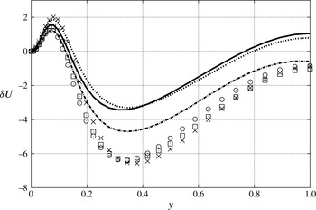
Forward approximation of DNS streamwise velocity perturbations for
 $Re=1450$
: ——,
 ${\it\epsilon}=0.005$
;
 $\times$
,
 ${\it\epsilon}=-0.005$
;
 $\cdots \cdots$
,
 ${\it\epsilon}=0.0025$
; ▫,
 ${\it\epsilon}=-0.0025$
; — ⋅ —,
 ${\it\epsilon}=0.00125$
;
 $\odot$
,
 ${\it\epsilon}=-0.00125$
.

The amplitude of the forcing-term coefficient
 ${\it\epsilon}$
is a delicate parameter, and must be accurately chosen to strike a balance between the linear response of the system and its statistical fluctuations: in our tested range that goes from
 $\pm 0.000625$
to
 $\pm 0.1$
, we empirically observe linear behaviour for
 ${\it\epsilon}=0.00125,0.0025,0.005$
.
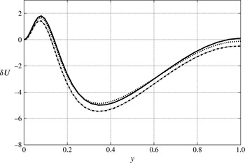
Figure 4 shows the profiles of DNS streamwise velocity perturbations for the most interesting values of
 ${\it\epsilon}$
, as obtained by using the forward approximation (4.16), while figure 5 depicts the same profiles as obtained with the central approximation (4.17). In the use of a forward approximation, the main differences are evident around the minimum of the curves even for cases with the same value of
 ${\it\epsilon}$
but different signs. The central approximation reduces the discrepancies and a linear behaviour is clearly more evident.
The length of computation necessary to obtain a sufficient reduction of statistical error makes it so that the largest part of the present results have been obtained for
 $Re=1450$
and
 $Re=1700$
even if, from a physical viewpoint, higher Reynolds number cases would have been interesting. All the time-averaged physical quantities are defined in the statistically stationary state, that is the state in which all multi-time statistics are invariant under a shift in time while the one-point statistics are independent of time. One of the greatest difficulties encountered in this work is represented by the computational time needed for convergence to a statistically stationary state, which is strongly influenced by the amplitude of the
 ${\it\epsilon}$
constant. By decreasing the value of
 ${\it\epsilon}$
, larger averaging times become necessary to obtain a statistically stationary state. As an example, for a bulk Reynolds number equal to 1450 and friction-velocity Reynolds number
 $Re_{{\it\tau}}=100$
, we observe that the case at
 ${\it\epsilon}=0.00125$
requires a very long calculation time to attain a statistically stationary state (approximately equal to
 $1.2\times 10^{6}$
time steps and a time step size of
 $0.02$
) and it is twice that with
 ${\it\epsilon}=0.0025$
.
By decreasing
 ${\it\epsilon}$
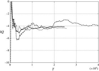
, larger averaging times become necessary to obtain a statistically stationary state. In order to better appreciate the convergence history, let us consider the flow rate perturbation in the case of constant pressure gradient as a function of averaging time
 $T$
, i.e.
 $$\begin{eqnarray}{\it\delta}Q=\frac{1}{T}\int _{0}^{T}\int _{0}^{1}{\it\delta}U\,\text{d}y\,\text{d}t.\end{eqnarray}$$
Figure 6 depicts the profile of
 ${\it\delta}Q$
for the above mentioned values of
 ${\it\epsilon}$
and
 $Re=1450$
. It shows that the case at
 ${\it\epsilon}=0.00125$
needs a longer convergence time for
 ${\it\delta}Q$
with respect to the other two cases.
Central approximation of DNS streamwise velocity perturbations for
 $Re=1450$
: ——,
 ${\it\epsilon}=0.005$
;
 $\cdots \cdots$
,
 ${\it\epsilon}=0.0025$
; — ⋅ —,
 ${\it\epsilon}=0.00125$
.

The convergence history of
 ${\it\delta}Q$
versus averaging time
 $T$
non-dimensionalized with the bulk velocity and the half height of the channel (CPG,
 $Re=1450$
): ——,
 ${\it\epsilon}=0.005$
;
 $\cdots \cdots$
,
 ${\it\epsilon}=0.0025$
; — ⋅ —,
 ${\it\epsilon}=0.00125$
.

4.4. Estimation of the variance of the numerical averaging
Figure 6 only provides a qualitative indication of the time required for the statistically stationary state to be attained. In order to have a more reliable result, it is important to have a quantitative estimation of the variance of all the averaged values. It is possible to verify that, for time series with integrable correlation function, such variances are inversely proportional to
 $\sqrt{T}$
, so they represent an important parameter that can provide a confidence interval for a given
 $T$
(see Hamilton Reference Hamilton1994).
Non-overlapping batch means (NOLBM) is a well-known approach for estimating the variance of averaged values of a discrete time series (see Meketon & Schmeiser Reference Meketon and Schmeiser1984). It is based on the subdivision of the total sample interval into a certain number of parts, whose time averages are called batch means. If
 $\bar{f}$
is the globally averaged value, the estimation of the standard deviation of it can be estimated as
 $$\begin{eqnarray}{\it\sigma}(\bar{f})=\sqrt{\frac{m}{n(b-1)}\mathop{\sum }_{j=1}^{b}(\bar{f}_{i,m}-\bar{f})^{2}},\end{eqnarray}$$
where
 $k$
is the number of contiguous, non-overlapping batches of observations, each of length
 $m$
, derived from the simulation-generated time series (assuming that
 $n=mb$
). For sufficiently large batch size
 $m$
, the batch means
 $$\begin{eqnarray}\bar{f}_{i,m}=\frac{1}{m}\mathop{\sum }_{k=1}^{m}f_{(i-1)m+k}\end{eqnarray}$$
become approximately independent and identically distributed normal random variables. All the results considered here will be accompanied with their corresponding standard deviations. An improved version of this method of estimating variances will be the subject of another paper under development.
5. Results
This section is devoted to the results obtained from the EVM and DNS in the calculation of the perturbation caused by external volume forces, and to their comparison. The constant-flow-rate cases differ from the constant-pressure-gradient configurations because in the latter, the relation between wall shear stress and
 $p_{x}$
remains the same before and after the perturbation, as already stated in § 2.
5.0.1. The constant-flow-rate case
DNS based and EVM calculation of perturbations of streamwise velocity versus the wall-normal coordinate (CFR, volume force 1):
 $\cdots \cdots$
, DNS (
 $Re=1450$
); — ⋅ —, EVM (
 $Re=1450$
);
 $\times$
, DNS (
 $Re=1700$
); ▫, EVM (
 $Re=1700$
).

DNS based and EVM calculation of perturbations of streamwise velocity versus the wall-units coordinate (CFR, volume force 1):
 $\cdots \cdots$
, DNS (
 $Re=1450$
); — ⋅ —, EVM (
 $Re=1450$
);
 $\times$
, DNS (
 $Re=1700$
); ▫, EVM (
 $Re=1700$
).

DNS perturbations of streamwise velocity, pressure gradient and wall shear stress (
 ${\it\delta}u$
,
 ${\it\delta}p_{x}$
and
 ${\it\delta}{\it\tau}$
) are evaluated using (4.17). The forcing term considered is defined by (2.2a
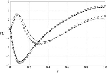
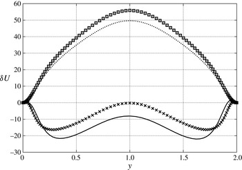
) in § 2. Figure 7 shows the comparison between the DNS and EVM velocity perturbations for two Reynolds numbers of 1450 and 1700: the results obtained with the eddy-viscosity model are very different from those derived from DNS, especially in the portion of the channel closest to the wall (
 $y=0$
), where the DNS response is positive while the EVM curve is negative. These figures also show that
 ${\it\delta}U$
according to DNS changes sign with respect to the forcing
 $F$
in the portion of the channel near to the wall. By increasing the Reynolds number, DNS curves of
 ${\it\delta}U$
tend to move towards the wall.
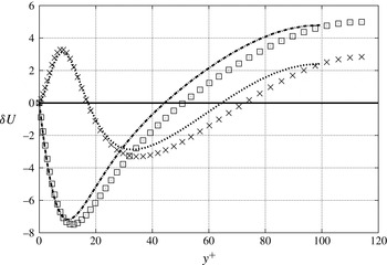
In order to better appreciate the dependence on the Reynolds number, the same curves are also plotted versus the non-dimensional wall distance
 $y^{+}=yu_{{\it\tau}}/{\it\nu}$
: figure 8 shows that there is a part of the channel in which the curves tend to overlap, the wall layer of the channel. Table 1 contains DNS and EVM perturbations of
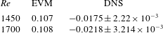
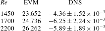
 $p_{x}$
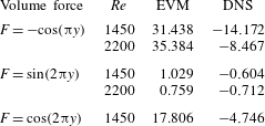
: they are opposite in sign, as well as being of different order of magnitude. The same table contains the values of the standard deviation calculated by using formula (4.19): this parameter gives an estimation of the error produced by the time average. For each Reynolds number, the standard deviation is one order of magnitude lower than the corresponding average value.
5.1. The constant-pressure-gradient case
Results in this section are obtained by keeping pressure gradient the same before and after the perturbation. Contrary to what happens in the constant-flow-rate case, the wall-shear-stress perturbation (
 ${\it\delta}{\it\tau}$
) will then also be zero. This also implies that properties of the turbulence in the wall layer will be mostly unaffected. Figures 9–11 refer to the volume force defined by (2.2a
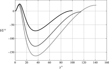
) in § 2. Figure 9 shows that the Reynolds number especially affects the portion of curve closest to the wall; in fact as the Reynolds number increases, curves tend to move towards to the wall. Just as in the constant-flow-rate case, the same curves are plotted versus
 $y^{+}$
in figure 10; here too there is a region where the curves overlap.
DNS-based perturbations of linear response of streamwise velocity in outer units (CPG, volume force 1): ——,
 $Re=1450$
; – – –,
 $Re=1700$
;
 $\cdots \cdots$
,
 $Re=2200$
.

Pressure gradient perturbations
 ${\it\delta}P_{x}$
.

DNS-based perturbations of linear response of streamwise velocity in wall units (CPG, volume force 1): ——,
 $Re=1450$
; – – –,
 $Re=1700$
;
 $\cdots \cdots$
,
 $Re=2200$
.

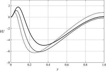
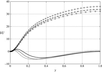
These curves are plotted again in figure 11, but now they are compared with the corresponding curves based on EVM. For all the Reynolds numbers, they only match in the viscous sublayer of the channel closest to the wall where physical viscosity is dominant and the wall shear stress is the same as in laminar flow. DNS and EVM results are completely different in the central part of the channel. In particular, DNS curves change sign along the height of the channel, whereas the EVM profiles are always positive. These results are also confirmed by the perturbations of flow rate
 ${\it\delta}Q$
, which are compared against each other in table 2: once again they are opposite in sign.
DNS and EVM calculation of perturbations of streamwise velocity versus the wall-normal coordinate (CPG, volume force
 $1$
): ——, DNS (
 $Re=1450$
); – – –, DNS (
 $Re=1700$
);
 $\cdots \cdots$
, DNS (
 $Re=2200$
); ▫, EVM (
 $Re=1450$
); ▵, EVM (
 $Re=1700$
);○, EVM (
 $Re=2200$
).

Perturbations of streamwise velocity (CPG, volume force 2): ——, DNS (
 $Re=1450$
);
 $\cdots \cdots$
, EVM (
 $Re=1450$
);
 $\times$
, DNS (
 $Re=2200$
); ▫, EVM (
 $Re=2200$
).

Flow rate perturbations
 ${\it\delta}Q$
.

5.2. Sinusoidal perturbations
From the preliminary results that we obtained with the volume force (2.2a
), we did not find a physical explanation for the trend of (
 ${\it\delta}U$
). In particular, the DNS velocity perturbation is not monotonic in the half height of the channel even though the volume force is an increasing function. Since the volume force (2.2a
) is related to a channel flow, to be more general, we decide to consider sinusoidal symmetric and antisymmetric forces, as representative of the first harmonics of a Fourier series. In this way, we are able to calculate
 ${\it\delta}U$
for a generic function and verify if the DNS velocity perturbation is influenced by the symmetry/antisymmetry of the volume forces.
Figure 12 refers to force (2.2b
), and depicts the profile of
 ${\it\delta}U$
versus the wall-normal coordinate
 $y$
obtained from DNS and EVM. The wall-normal coordinate now goes from one wall to the other in order to observe whether the symmetry of the volume force is inherited by the corresponding velocity profile. Just as before, curves can be overlapped only in the viscous sublayer of the channel closest to the wall, while they are quite different in the central part of the channel.
Figure 13 depicts a profile of
 ${\it\delta}U$
versus the wall-normal coordinate
 $y$
obtained from DNS and EVM when the volume force is (2.2c
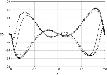
). For all the Reynolds numbers, the curves can be observed to be approximately antisymmetric with respect to the centre of the channel (the slight discrepancy being due to statistical error), owing to the application of an antisymmetric force. Once again they can be overlapped only in the portion of the channel closest to the wall, while they are quite different in its central part.
Figure 14 depicts the profile of
 ${\it\delta}U$
versus the wall-normal coordinate
 $y$
obtained from DNS and EVM in the case of the volume force (2.2d
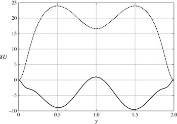
). Curves can be overlapped only in the viscous sublayer of the channel closest to the wall, while they are quite different in the central part of the channel. All these results are also confirmed by DNS-based and EVM calculations of
 ${\it\delta}Q$
, which are compared in table 3: once again they are opposite in sign.
Perturbations of streamwise velocity (CPG, volume force 3): ——, DNS (
 $Re=1450$
);
 $\cdots \cdots$
, EVM (
 $Re=1450$
);
 $\times$
, DNS (
 $Re=2200$
); ▫, EVM (
 $Re=2200$
).

Perturbations of streamwise velocity (CPG, volume force 4): ——, DNS (
 $Re=1450$
);
 $\cdots \cdots$
, EVM (
 $Re=1450$
).

Flow rate perturbations
 ${\it\delta}Q$
.

5.3. Could a different eddy viscosity have matched the DNS results?
The previous sections have demonstrated that the algebraic eddy-viscosity model (4.9) cannot reproduce DNS in calculating the response of turbulent flow to a volume force. However a different eddy viscosity might be able to do it. In order to verify this possibility we can reverse (4.10), and use it to determine an eddy-viscosity profile from the known velocity perturbation provided by DNS:
 $$\begin{eqnarray}{\it\nu}_{e}=\frac{\displaystyle \int _{0}^{y}F\,\text{d}y}{{\it\delta}U_{y,dns}},\end{eqnarray}$$
where
 ${\it\delta}U_{y,dns}$
is the
 $y$
-derivative of
 ${\it\delta}U_{dns}$
and
 $F$
is the volume force of (2.2a
). The numerator of (5.1) is positive for every
 $y$
; since
 ${\it\delta}U_{y,dns}$
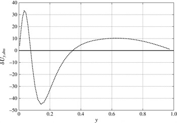
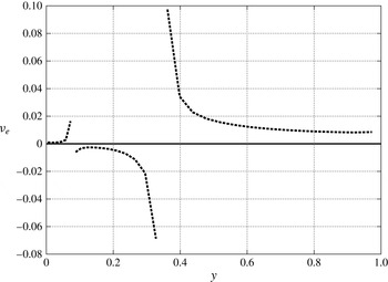
has alternating sign (see figure 15), this would lead to a negative eddy viscosity in some parts of the channel (figure 16), hardly a physically acceptable result. In addition, where
 ${\it\delta}U_{y,dns}$
changes sign (at two points of the channel), the eddy viscosity according to (5.1) tends to infinity. As a conclusion, (5.1) is unacceptable. Conversely, it can also be proved that any non-negative eddy viscosity inserted into (4.10) would produce a monotonically increasing velocity perturbation, and therefore could never approach the observed behaviour of
 ${\it\delta}U_{dns}$
.
 $Y$
-derivative of
 ${\it\delta}U_{dns}$
.

Eddy-viscosity profile generated from
 ${\it\delta}U_{dns}$
.

6. Conclusions
A benchmark problem has been devised simple enough that it allows a head-to-head comparison between the eddy-viscosity model and DNS of the same problem within a family. This is the linear response of turbulent channel flow to a
 $y$
-dependent external volume force. The physical domain is the classical plane channel, bounded by two parallel walls and characterized by two homogeneous directions. The flow has been forced by an external volume force whose integral in the wall-normal direction is zero, because its constant part can always be absorbed in the streamwise pressure gradient. The main aim of this work has been the comparison between the eddy-viscosity model and DNS of the linear response of turbulent flow to an external volume force. Different profiles of forcing have been considered: the volume force described in appendix A and relevant to Luchini & Charru (Reference Luchini and Charru2010b
), and a few cases of sinusoidal forces. Since this is parallel flow, most possible turbulence models would reduce to an algebraic eddy-viscosity model anyway; we have used the one adopted by Luchini & Charru (Reference Luchini and Charru2010b
).
The laminar case of forced plane channel is amenable to a completely analytical solution of the problem. The results have demonstrated that the linear response of streamwise velocity is positive everywhere in the channel and a flow rate is generated with no net reaction.
In the case of turbulent flow, the computation time required for convergence of the results to a statistically stationary state is the limiting factor, and strongly depends on the
 ${\it\epsilon}$
coefficient determining the amplitude of the volume force. Most results have been limited to
 $Re=1450$
and
 $Re=1700$
in order to contain computation time within reasonable limits, although from a physical point of view, higher Reynolds numbers would also have been interesting.
The computational averaging time required to attain a statistically stationary state becomes larger and larger as the
 ${\it\epsilon}$
constant is decreased. The amplitude
 ${\it\epsilon}$
of the forcing term must strike a delicate balance between this effect and linearity of the response of the system: in the range that goes from
 ${\it\epsilon}=0.000625$
to
 ${\it\epsilon}=0.1$
, a linear behaviour has been verified for
 ${\it\epsilon}=0.00125;0.0025;0.005$
. To better assess the reliability of such averaged values obtained over the longer time, an estimation of their variance has been made by the method of NOLBM.
All the results from both EVM and DNS have been calculated both with an imposed constant flow rate and constant pressure gradient in the streamwise direction. In the constant-flow-rate case, DNS perturbations of streamwise velocity are very different from those derived from EVM, especially near the wall, where the DNS profile of
 ${\it\delta}U$
changes sign with respect to the forcing
 $F$
. The same curves have also been plotted versus
 $y^{+}$
in order to verify if there is a wall scaling in their Reynolds-number dependence: in a suitable region near the wall, the two curves do tend to overlap. These differences have been confirmed by the values of
 ${\it\delta}P_{x}$
which turn out to be opposite in sign, as well as being of different order of magnitude. In the constant-pressure-gradient case, the differences between the EVM and DNS profiles of
 ${\it\delta}U$
are even larger than in the constant-flow-rate case. For all the Reynolds numbers, curves overlap only in the viscous sublayer of the channel closest to the wall, where shear stress is exactly the same as the laminar case, while they are very different in the central part of the channel. These results have been confirmed by DNS and EVM calculations of
 ${\it\delta}Q$
: once again they are opposite in sign.
The general outcome of this paper is that no eddy-viscosity model can reproduce DNS in calculating the response of turbulent flow to a volume force. In addition to providing evidence for the particular model tested, it has been demonstrated that it is not possible to generate a new eddy-viscosity model that can reproduce the DNS perturbation curve of streamwise velocity, unless negative and even infinite viscosity is allowed.
Acknowledgements
This work was supported by the INSIST project, and partially by the Institut de Mècanique des Fluides de Toulouse through research invitations.
Appendix A. Connection with the problem of flow past an undulated wall
The linear response of channel flow to an external volume force is linked to the problem of the motion of a fluid past an undulated wall. This last topic is of interest in the context of the dynamics and possible destabilization of an erodible bed. A few relevant papers are the following, in particular in so far as they deal with the degree of linearity of the wall shear stress with respect to the amplitude of the wall oscillations and make comparisons with some turbulence models.
Zilker, Cook & Hanratty (Reference Zilker, Cook and Hanratty1977) made measurements of the shear-stress variation along and the velocity profiles above a wavy wall bounding a turbulent flow for geometries with height-to-length ratios of
 $2{\it\epsilon}/{\it\lambda}=0.0312$
and
 $0.05$
, where
 ${\it\epsilon}$
is the amplitude of the sinusoidal wall modulation and
 ${\it\lambda}$
its wavelength. They observed a linear behaviour for the case of
 $2{\it\epsilon}/{\it\lambda}=0.0312$
, because the shear stress could be described quite well by a single harmonic with a wavelength equal to that of the surface. Moreover they also suggested that the linear behaviour depends on the value of
 ${\it\epsilon}u_{{\it\tau}}/{\it\nu}$
, where
 $u_{{\it\tau}}$
and
 ${\it\nu}$
are, respectively, the wall velocity and the kinematic viscosity, and it is ensured when
 ${\it\epsilon}u_{{\it\tau}}/{\it\nu}<27$
.
Frederick & Hanratty (Reference Frederick and Hanratty1988) used a laser-Doppler velocimeter to obtain measurements of the streamwise velocity over sinusoidal walls characterized by a small amplitude, with
 $2{\it\epsilon}/{\it\lambda}=0.0312$
. These results were compared with numerical calculations based on the Reynolds-averaged Navier–Stokes equations with the van Driest model for the mixing length. They observed that the eddy-viscosity model successfully described very well the wall shear stress and the wall-induced velocity variations, while the velocity field agrees roughly with what is measured. Moreover, they found a threshold value for
 ${\it\epsilon}u_{{\it\tau}}/{\it\nu}$
of
 $12$
, less than the value of
 $27$
suggested by Zilker as a requirement for linear behaviour of a non-separated flow. This difference can be attributed to the use of an eddy-viscosity relationship that gives a good fit of the velocity field for turbulent flow in a flat-walled channel. Abrams (Reference Abrams1979) and McLean (Reference McLean1983) had already noted that turbulence models developed to provide agreement with the results regarding surface shear stress amplitude and phase angles do not correctly predict nonlinear effects observed in the wall shear stress measurements on large amplitude waves.
Henn & Sykes (Reference Henn and Sykes1999) used large-eddy simulation to investigate fully-developed turbulent flow in a channel wherein the lower wall is sinusoidal and
 $2{\it\epsilon}/{\it\lambda}=0.0312$
. The model predictions were close to the measurements in both phase and magnitude, although a little scatter was observed in experimental data. With respect to Frederick & Hanratty (Reference Frederick and Hanratty1988), they found a slightly smaller phase shift between the dominant first harmonic of the wall shear stress and the wall profile. All of the above mentioned papers have observed a phase lead of the wall shear stress relative to the wall modulation. Fitting the data with a two-harmonics Fourier series, Frederick et al. found a phase lead of 51° for the dominant first harmonic; while the LES showed a slightly smaller phase shift of approximately 45°.
Luchini & Charru (Reference Luchini and Charru2010b ) applied a perturbative expansion to the Reynolds-averaged Navier–Stokes equations in order to simulate the effect of a slowly varying wall geometry, by providing consistent corrections to the bottom shear stress and pressure gradient associated with slow changes in the water depth. A key step in the procedure of Luchini & Charru (Reference Luchini and Charru2010b ) was the reduction of the effect of the slowly varying depth to an equivalent volume force. A summary of this procedure now follows.
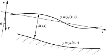
Sketch of the free-surface channel with a variable bottom.

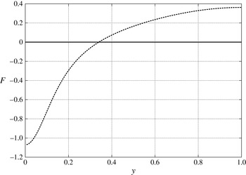
Profile of the volume force relevant to Luchini & Charru (Reference Luchini and Charru2010b
)(
 $Re=1700$
).

Flow in a domain with a slowly varying wall geometry (figure 17) is described by the boundary-layer equations because the transverse velocity, normal to the boundary, is much smaller than the characteristic streamwise velocity. Moreover, it is characterized by a thickness much smaller than the streamwise characteristic length over which the same thickness varies. Under these assumptions, if superscript symbol
 $^{\ast }$
is used for dimensional quantities, the Navier–Stokes equations of turbulent incompressible flow reduce to Prandtl’s boundary-layer equations, i.e.
 $$\begin{eqnarray}\left.\begin{array}{@{}c@{}}u_{x^{\ast }}^{\ast }+v_{y^{\ast }}^{\ast }=0,\\ u_{t^{\ast }}^{\ast }+u^{\ast }u_{x^{\ast }}^{\ast }+v^{\ast }u_{y^{\ast }}^{\ast }+p_{x^{\ast }}^{\ast }={\it\tau}_{y^{\ast }}^{\ast },\\ p_{y^{\ast }}^{\ast }=0,\end{array}\right\}\end{eqnarray}$$
 $u^{\ast }$
and
 $v^{\ast }$
respectively denote the
 $x^{\ast }$
and
 $y^{\ast }$
component of velocity. The boundary conditions are
 $$\begin{eqnarray}u_{y^{\ast }}^{\ast }(x^{\ast },0,t^{\ast })=v^{\ast }(x^{\ast },0,t^{\ast })=u^{\ast }(x^{\ast },-h^{\ast },t^{\ast })=0;\quad v^{\ast }(x^{\ast },-h^{\ast },t^{\ast })=-h_{t^{\ast }}^{\ast }\end{eqnarray}$$
(where
 $h_{t}^{\ast }$
will be zero for the present purposes).
In Luchini & Charru (Reference Luchini and Charru2010b
),
 $h_{x}^{\ast }$
but not necessarily
 $h^{\ast }$
is assumed to be small. At order 0 with respect to
 $h_{x^{\ast }}^{\ast }$
, the solution
 $u^{\ast (0)}$
may be written as
 $u^{\ast (0)}=h^{\ast -1}U^{\ast }(z)$
, where
 $z=y^{\ast }/h^{\ast }(x^{\ast })$
and the prefactor
 $h^{\ast -1}$
is required by continuity.
 $U^{\ast }(z)$
is proportional to
 $1-z^{2}$
in laminar Poiseuille flow, or may more generally be assumed to be whatever the unperturbed velocity profile is in a turbulent flow. At order 1, equation (3.3) of Luchini & Charru (Reference Luchini and Charru2010b
) is obtained from (A 1), i.e.
 $$\begin{eqnarray}{\it\tau}_{y^{\ast }}^{\ast (1)}-{\it\rho}^{\ast -1}P_{x^{\ast }}^{\ast (1)}=u^{\ast (0)}u_{x^{\ast }}^{\ast (0)}+v^{\ast (1)}u_{y^{\ast }}^{\ast (0)}=u^{\ast (0)}u_{x^{\ast }}^{\ast (0)}-u_{y^{\ast }}^{\ast (0)}\int _{0}^{y^{\ast }}u_{x^{\ast }}^{\ast (0)}\,\text{d}y^{\ast }.\end{eqnarray}$$
For the given expression of
 $u^{\ast (0)}=h^{\ast -1}U^{\ast }(z)$
,
 $$\begin{eqnarray}\displaystyle h^{\ast -1}{\it\tau}_{z}^{\ast (1)}-{\it\rho}^{\ast -1}P_{x^{\ast }}^{\ast (1)} & \hspace{-2.0pt}=\hspace{-2.0pt} & \displaystyle -\frac{h_{x^{\ast }}^{\ast }}{h^{\ast 3}}U^{\ast }\,(U^{\ast }+zU_{z}^{\ast })+\frac{h_{x^{\ast }}^{\ast }}{h^{\ast 3}}\,U_{z^{\ast }}^{\ast }\int _{0}^{z^{\ast }}\,(U^{\ast }+zU_{z}^{\ast })\,\text{d}z\nonumber\\ \displaystyle & \hspace{-2.0pt}=\hspace{-2.0pt} & \displaystyle -\frac{h_{x^{\ast }}^{\ast }}{h^{\ast 3}}U^{\ast }\,(U^{\ast }+zU_{z}^{\ast })+\frac{h_{x^{\ast }}^{\ast }\,U_{z}^{\ast }}{h^{\ast 3}}\,zU^{\ast }=-\frac{h_{x^{\ast }}^{\ast }}{h^{\ast 3}}U^{\ast 2}.\end{eqnarray}$$
The closure of this equation was obtained by Luchini & Charru (Reference Luchini and Charru2010b
) through a turbulence model for the shear stress,
 ${\it\tau}^{(\ast 1)}$
. However, (A 4) is also clearly the same that would be obtained at first order by perturbing a straight-channel flow with a volume force proportional to
 $U^{\ast 2}(y)$
. Considering that an additive constant in the right-hand side will be immediately absorbed by the pressure-gradient perturbation
 $P_{x^{\ast }}^{\ast (1)}$
, we may always normalize this equivalent force so as to have zero mean. Therefore the right-hand-side forcing equivalent to a channel-wall perturbation, used elsewhere in this paper, is
 $$\begin{eqnarray}F(y)=U^{2}(y)-\{U^{2}\},\end{eqnarray}$$
(figure 18) where, in a DNS of a plane channel flow with
 $x$
and
 $z$
as the homogeneous directions,
 $U(y)$
is the
 $x$
-,
 $z$
- and time-averaged streamwise velocity and
 $\{\cdot \}$
denotes a mean value in the
 $y$
direction.