



1. Introduction
Let
 $(X,0) \subset \mathbb{C}^N$
be a complex surface germ with an isolated normal singular point at the origin. The link Y of (X, 0) is the smooth 3-manifold
 $Y = X \cap \,S_r^{2N-1}$
obtained by intersecting X with a sphere of small radius
 $r\gt0$
centered at 0. The link Y carries a canonical contact structure given by the distribution of complex tangencies to Y. The contact link
 $(Y, \xi)$
is independent of the choice of r, up to contactomorphism. The link
 $(Y, \xi)$
can also be described as the convex boundary of the negative definite plumbing of symplectic disc bundles over surfaces, given by a neighborhood of the exceptional divisor in any resolution of (X, 0).
In this article, we examine symplectic and Stein fillings of
 $(Y, \xi)$
and their relation to smoothings of surface singularities with the given boundary link. Suppose that
 $\lambda\colon (X, 0) \to (T, 0)$
is a one-parameter smoothing, so that
 $X_t:= \lambda^{-1}(t)$
is smooth for
 $t\neq 0$
. It is known that the diffeomorphism type and the Stein homotopy type of
 $X_t$
is independent of t; we refer to
 $X_t$
as the Milnor fiber associated to the smoothing
 $\lambda$
. Intersecting with a small ball centered at the origin, we can also think of a compact version of the Milnor fiber: this is a compact Stein domain W whose contact boundary is given by
 $(Y, \xi)$
. These, together with the minimal resolution of the singularity, whose symplectic structure can be deformed into a Stein structure by [Reference Bogomolov and de OliveiraBdO97], can be thought of as Stein fillings of algebro-geometric origin. (If the singularity is rational, we do not need to consider the resolution separately, as the corresponding filling arises from the Artin smoothing.) We will refer to these fillings as Milnor fillings, even though the term is often used for singular surface germs in the literature. It is interesting to compare Milnor fillings to the more general Stein fillings of
 $(Y, \xi)$
. These two collections of fillings are known to coincide in certain simple cases, such as lens spaces (arising as links of cyclic quotient singularities) [Reference LiscaLis08, Reference Némethi and Popescu-PampuNP10b], and more generally, links of quotient singularities [Reference Park, Park, Shin and UrzúaPPS+18, Reference Bhupal and OnoBO12], and links of simple elliptic singularities [Reference Ohta and OnoOO03, Reference Ohta and OnoOO05]. However, for general singularities, they can be different [Reference Akhmedov and OzbagciAO14, Reference Akhmedov and OzbagciAO18, Reference Plamenevskaya and StarkstonPS23].
As a first ground of comparison, we prove that the Milnor fillings of a fixed link have bounded topology.
Theorem 1.1.
Let
 $(Y, \xi)$
be the contact link of a normal surface singularity (X,0). Then, the Euler characteristic, the signature,
 $b_2^+$
and
 $b_2^-$
of all Milnor fillings of
 $(Y, \xi)$
are bounded by a constant that depends only on the link.
Note that in the discussion and proof of Theorem 1.1 and related results such as Theorem 1.4, we can focus on Milnor fibers and ignore the minimal resolution since it only adds one element to the set of Milnor fillings, considered up to diffeomorphism. We will be careful to mention the minimal resolution when it is important.
The statement of Theorem 1.1 is manifestly false for general Stein fillings of links; monodromy techniques as in [Reference Baykur and Van Horn-MorrisBV15, Reference Baykur and Van Horn-MorrisBV16, Reference Baykur, Monden and Van Horn-MorrisBMV17, Reference Dalyan, Korkmaz and PamukDKP15] produce collections of Stein fillings with unbounded topology for many non-rational singularities. We will come back to this point shortly.
It is important to note that in Theorem 1.1, we fix the link
 $(Y, \xi)$
, which amounts to fixing only the topological type of the surface singularity. A given topological type may support infinitely many analytic types (X, 0). In fact, this is almost always the case: topological types that support a unique (respectively finitely many) analytic structures satisfy very restrictive constraints on their resolution graphs [Reference LauferLau73]. These are called taut (respectively pseudotaut); most singularities are not (pseudo)taut. For a fixed analytic type (X, 0), there are only finitely many Milnor fibers, but different analytic types may produce non-diffeomorphic Milnor fibers. By [Reference Caubel, Némethi and Popescu-PampuCNP06], all these Milnor fibers induce the unique Milnor-fillable contact structure
 $\xi$
on the link, which in fact can be identified as the boundary of the plumbing of symplectic disc bundles given by the resolution [Reference Gay and StipsiczGS09]. The resulting collection of Milnor fillings may a priori be infinite. We do not know if an infinitude of Milnor fillings can actually exist, but for sandwiched singularities, an important subclass of rational singularities, we are able to prove the finiteness of Milnor fillings, sharpening Theorem 1.1 for this class. Note that most sandwiched singularities are not (pseudo)taut.
Theorem 1.2. The contact link of a sandwiched surface singularity admits only finitely many Milnor fillings, up to diffeomorphism.
The proof is based on a dimensional reduction due to de Jong and van Straten [Reference de Jong and van StratendJvS98]. A sandwiched singularity can be characterized via an associated germ of a singular plane algebraic curve, and the Milnor fibers can be described via appropriate deformations of the curve germ. For curves, the parameter space of the analytic structures in a given topological type is finite-dimensional and much better understood. This enables us to prove Theorem 1.2 by working with the corresponding parameter space for all analytic structures in the given topological type of the singularity.
Moving on to Stein fillings of links, we probe the following problem.
Question 1.3 [Reference NémethiNém99]. For which contact links of normal surface singularities is every Stein filling diffeomorphic to a Milnor filling or the minimal resolution?
As in [Reference Plamenevskaya and StarkstonPS23], we are going to call a Stein filling of a link unexpected if it is not diffeomorphic to any Milnor filling or the minimal resolution, though a takeaway from our work here will be that one should generally ‘expect the unexpected’ in this context.
The examples of unexpected fillings we build in this article will come from monodromy factorizations through a variety of manipulations. Recall that a factorization of the monodromy of the supporting open book on a contact 3-manifold into a product of positive Dehn twists gives rise to a Lefschetz fibration. Provided all the Dehn twist curves in the factorization are homologically essential curves on the fiber, the allowable Lefschetz fibration carries a Stein structure and provides a filling of the contact manifold.
Theorem 1.1 implies that whenever the link admits a family of Stein fillings with unbounded topology, all but finitely many of these fillings will be unexpected. Examples of monodromies with arbitrarily long factorizations given in [Reference Baykur and Van Horn-MorrisBV16, Reference Baykur, Monden and Van Horn-MorrisBMV17, Reference Dalyan, Korkmaz and PamukDKP15] produce Stein fillings with arbitrarily high Euler characteristic. This approach works for a large family of singularities with dual-resolution graphs as in the next theorem. Every normal surface singularity has a good resolution where all exceptional curves are smooth, and all intersections between exceptional curves occur in transverse double points only.
Theorem 1.4. Suppose that (X, 0) is a normal surface singularity with a good resolution such that:
-
(i) for every irreducible exceptional curve E, its self-intersection
 $E \cdot E$
and the number a(E) of intersections with the other exceptional curves satisfy the inequality (1.1)
\begin{equation} a(E) \leqslant - E \cdot E;\end{equation}
-
(ii) there is an exceptional curve
$E_0$
of genus
$g\geqslant 4$
such that
$- E_0 \cdot E_0 \leqslant 2g -4$
. -
(iii) Then, the link
$(Y, \xi)$
of (X, 0) has infinitely many Stein fillings that are not homotopy equivalent to any Milnor fibers of any normal surface singularities with the given link. For an infinite family of graphs, there are such Stein fillings with
$b_1=0$
.


A deep result of Greuel and Steenbrink [Reference Greuel and SteenbrinkGS83] tells us that any Milnor fiber W of a normal surface singularity has vanishing first Betti number, which gives a way to argue that certain Stein fillings cannot come from Milnor fibers [Reference Akhmedov and OzbagciAO14]. Many of our unexpected fillings pass the Greuel–Steenbrink test.
The proof of Theorem 1.1 is based on the classical formulas of Laufer, Durfee and Wahl [Reference DurfeeDur78, Reference LauferLau77b, Reference SteenbrinkSte83, Reference WahlWah81] expressing the Euler characteristic and signature of Milnor fibers in terms of the geometric genus of the singularity. The geometric genus depends on the analytic structure, and thus in general is not determined by the link, but it satisfies topological upper bounds that yield the result for all Milnor fillings. These upper bounds, and therefore those of Theorem 1.1, can be computed from the resolution graph in specific examples. We can get explicit unexpected fillings in Theorem 1.4 by producing monodromy factorizations that violate these bounds. A simple family is the hypersurface singularity
 $\{x^p+y^p+z^p=0\} \subset \mathbb{C}^3$
. When
 $p\geqslant 5$
, its minimal resolution has an exceptional divisor consisting of a single curve E of genus
 $g=\frac12(p-1)(p-2)\gt2$
, with self-intersection
 $-b=-p$
. The link is the total space of an oriented
 $S^1$
-bundle over
 $\Sigma_g$
with Euler number
 $-b$
, equipped with the Boothby–Wang contact structure, which is supported by an open book whose page has genus g and b boundary components, and the monodromy is a boundary multitwist. This monodromy admits arbitrarily long factorizations into Dehn twists along homologically essential curves [Reference Baykur, Monden and Van Horn-MorrisBMV17], generating an infinite family of unexpected fillings with arbitrarily large topology.
The singularities in Theorem 1.4 are all non-rational, due to the presence of the higher-genus exceptional curves. For links of rational singularities, which are defined as singularities of geometric genus
 $p_g=0$
, the topology of general Stein fillings is quite restricted. From the topological perspective, these links are characterized as L-spaces in the sense of Heegaard Floer or monopole Floer homology [Reference NémethiNém17]. In this case, all Stein, and more generally, all minimal symplectic fillings are known to be negative definite, with uniformly bounded topology [Reference Ozsváth and SzabóOS04, Reference StipsiczSti03]. Nonetheless, unexpected fillings often exist, even in the most restricted case of rational singularities with reduced fundamental cycle, which can be characterized by having contact links supported by planar open books [Reference Némethi and TosunNT10, Reference Ghiggini, Golla and PlamenevskayaGGP20]. For links of such singularities, unexpected fillings were constructed in [Reference Plamenevskaya and StarkstonPS23]. (Note that in that paper, the unexpected fillings were distinguished from the Milnor fibers only relative to certain boundary data, but one can detect them in the absolute sense by using standard facts on the mapping-class group of the link, [Reference Plamenevskaya and StarkstonPS25].) Some of these unexpected fillings and Milnor fibers are simply connected and have negative definite intersection forms of the same rank.
The next interesting class is minimally elliptic singularities, which are Gorenstein singularities of geometric genus
 $p_g=1$
. If we additionally assume that the link is a rational homology sphere, then the links of such singularities are almost L-spaces in the terminology of Heegaard Floer or monopole Floer homology, and by the work of Lin [Reference LinLin20], the indefinite Stein fillings of each link all have the same Euler characteristic and signature. Lin’s results do not cover the negative-definite case, and it is intriguing that we can find such unexpected fillings distinguished by the rank of their intersection forms, using further constraints on the topology of Milnor fibers due to Laufer.
Theorem 1.5. There are infinite families of minimally elliptic singularities whose links admit Stein fillings that cannot be homotopy equivalent to a Milnor fiber or the minimal resolution. The examples include non-smoothable cusp singularities and triangle singularities.
Minimally elliptic singularities with reduced fundamental cycle (in their minimal resolution) are known to fall into three special subclasses of singularities: simple elliptic, cusp, and triangle singularities. In the case of simple elliptic singularities, which by definition have a resolution with a single exceptional curve of genus 1, every minimal symplectic filling of the contact link is diffeomorphic to a Milnor fiber or the minimal resolution by the work of Ohta and Ono [Reference Ohta and OnoOO05]. Thus, they constitute a class with a positive answer to Question 1.3. In contrast, we establish that there are many links of non-smoothable cusp singularities (which therefore admit no Milnor fibers) that admit Stein fillings not diffeomorphic to the minimal resolution, as well as many links of (smoothable) triangle singularities that also admit unexpected Stein fillings.
Upon closer examination, however, one notices that at least some of our examples in Theorem 1.5 could still be expected from the algebro-geometric viewpoint. Indeed, as symplectic fillings, these manifolds are obtained by symplectic rational blowdown, and it is plausible that on the algebraic side they can be generated via P-resolutions [Reference KollárKol91]. (This was pointed out to us by Paul Hacking.) It would be interesting to know if Theorem 1.1 extends to this case, that is, if the collection of fillings generated by P-resolutions has bounded topology.
In all the examples of unexpected Stein fillings discussed above for rational and minimally elliptic singularities, where we know that the Stein fillings of the links necessarily have uniformly bounded topology, we only had a finite collection of examples for each given link. This brings up the more general question of whether any contact 3-manifold with uniform bounds on the topology of its Stein fillings can have only finitely many Stein fillings, up to diffeomorphism [Reference Baykur and Van Horn-MorrisBV15]. Infinite collections of fillings for links of rational singularities seem particularly hard, or perhaps impossible to generate.
Question 1.6. Is there a link of rational singularity that admits infinitely many, pairwise non-diffeomorphic Stein fillings? Minimal symplectic fillings?
We may more generally ask if there are any L-spaces that admit infinitely many Stein fillings; no examples are known. Finiteness results are only available for some special cases, such as lens spaces, where fillings have been fully classified [Reference LiscaLis08]. Otherwise, the question is open even for rational singularities with reduced fundamental cycle.
Instead of Stein fillings, one may more generally consider minimal symplectic fillings. For some classes of contact 3-manifolds, such as the planar ones, the collections of Stein fillings and minimal symplectic fillings coincide (we consider fillings up to a diffeomorphism). In particular, all minimal symplectic fillings of lens spaces are given by Milnor fibers. However, in general, minimal symplectic fillings are much easier to generate: even in the minimally elliptic case when Stein fillings have bounded topology, we can easily construct symplectic fillings with arbitrarily large Euler characteristics. These can be obtained by taking a symplectic fiber sum [Reference GompfGom95] along an embedded symplectic torus of square zero in a Stein filling W of
 $(Y, \xi)$
, where minimality can be argued using [Reference UsherUsh06] and [Reference Lisca and MatičLM97]. Moreover, one can perform knot surgery [Reference Fintushel and SternFS98] with fibered knots along such torus to produce exotic copies. It is worth noting that this construction does not work for rational singularities; the presence of a square zero symplectic torus in a Stein filling W implies that W has an indefinite intersection form, which cannot be the case when the singularity is rational. This fact, together with the relation to taut foliations discussed below, underscores the challenge in getting potential examples for Question 1.6.
The existence of infinite collections of minimal symplectic fillings is related to taut foliations and the L-space conjecture [Reference BoyerBGW13], as we were reminded by Jeremy Van Horn-Morris. A link of a normal surface singularity is an L-space if and only if the singularity is rational [Reference NémethiNém17]. The L-space conjecture was proved in [Reference Hanselman, Rasmussen, Rasmussen and WatsonHRR+20, Reference RasmussenRas17] for all graph manifolds; it follows that link Y carries always a taut foliation in the non-rational case. One can then get a symplectic structure on
 $Y \times [-1, 1]$
and cap off
 $Y \times \{-1\}$
by a concave filling à la Eliashberg [Reference EliashbergEli04], which results in a (convex) symplectic filling for
 $Y \times \{1\}$
. Moreover, one can use different concave fillings (with arbitrarily large Euler characteristics) to get infinitely many different minimal symplectic fillings. (In general, one needs to check that the canonical contact structure on the link is obtained as a perturbation of the taut foliation. This would be automatic in examples where the tight contact structure is unique, e.g. for
 $Y=\Sigma(2, 3, 6m+1)$
, see [Reference Mark and TosunMT18]. For Seifert fibered spaces over
 $S^2$
, one can use a transverse taut foliation to get a transverse contact structure
 $\xi$
, see [Reference Lisca and StipsiczLS07], so
 $\xi$
must be canonical by [Reference Caubel, Némethi and Popescu-PampuCNP06].)
It is often conjectured that planar contact 3-manifolds admit only finitely many minimal symplectic fillings, up to symplectic deformation [Reference Lisi and WendlLW21]. One might conjecture that finiteness of fillings generally holds for all rational singularities, or even for all L-spaces.
1.1 Organization of the paper
We discuss the constraints on the topological invariants of Milnor fibers in § 2 and prove Theorem 1.1. We prove Theorem 1.4 in § 3 and present, for certain families of links, explicit examples of non-Milnor Stein fillings with arbitrarily large topology. Section 4 is where we consider the minimally elliptic singularities and construct many examples of unexpected Stein fillings to prove Theorem 1.5. In § 5, we show that there are finitely many Milnor fillings of a sandwich singularity, proving Theorem 1.2.
2. Proof of Theorem 1.1
We first recall some useful inequalities that follow from the exact sequence of the pair
 $(W, \partial W)$
, where W is a Stein filling of the link
 $Y= \partial W$
. Since W is Stein and so
 $H_3(W)=0$
and
 $H_1(W, \partial W)= H^3(W)=0,$
we have
 \begin{align*}0 \rightarrow H_3(W, \partial W) \stackrel{\partial_*}{\longrightarrow} H_2 (\partial W) \stackrel{i_*}{\longrightarrow} H_2(W) \longrightarrow H_2 (W, \partial W) \longrightarrow H_1 (\partial W) \longrightarrow H_1 (W) \rightarrow 0.\end{align*}
Then,
 \begin{equation}b_1(W)\leqslant b_1(\partial W) = b_1(Y).\end{equation}
Furthermore, the intersection form
 $Q_W$
is zero on
 $i_*(H_2(\partial W))$
, and, moreover, by the Poincaré–Lefschetz duality,
 $i_*(H_2(\partial W))$
is the maximal subspace of
 $H_2(W)$
where
 $Q_W$
is zero. Therefore,
 \begin{equation}b_2^0(W)= \operatorname{rk} i_*(H_2(\partial W))=\operatorname{rk} H_2(\partial W) - rk H_3 (W, \partial W) = b_1(\partial W) - b_1(W);\end{equation}
we used the fact that
 $\partial_*$
is injective. It follows that
 \begin{equation} b_2^0(W) \leqslant b_1(Y)\end{equation}
for every Stein filling of the link Y. When W is a Milnor fiber,
 $b_1(W)=0$
by [Reference Greuel and SteenbrinkGS83], so in that case
 \begin{equation}b_2^0(W)=b_1(Y).\end{equation}
We are going to use the following result of Stipsicz [Reference StipsiczSti03] providing uniform bounds on the topology of arbitrary Stein fillings.
Proposition 2.1 [Reference StipsiczSti03, Theorem 1.4]. For a given contact 3-manifold
 $(Y, \xi)$
, the quantity
 $2\chi(W)+3 \sigma(W)$
is bounded below as W ranges over all Stein fillings of
 $(Y, \xi)$
.
Remark 2.2. If
 $(Y, \xi)$
is given by an open-book decomposition, and one considers a family of Stein fillings given by monodromy factorizations, it is possible to give explicit bounds in the above statement. For example, let
 $Y_{g,b}$
be an oriented
 $S^1$
-bundle over
 $\Sigma_g$
with Euler number
 $-b$
with its Boothby–Wang contact structure, as at the end of the previous section. It is supported by the open book with page
 $\Sigma_g^b$
and monodromy the boundary multitwist
 $\Delta$
in the mapping class group
 $\operatorname{Mod}(\Sigma_g^b)$
. Capping off every boundary component of this open book a là Eliashberg [Reference EliashbergEli04], we obtain a symplectic cobordism to a
 $\Sigma_g$
-bundle over
 $S^1$
with trivial monodromy. The latter can be symplectically capped off with a symplectic trivial
 $\Sigma_g$
-bundle over
 $\Sigma_1^1$
. This way, we generated a concave cap
 $\mathcal{C}$
for
 $Y_{g,b}$
. Now, let X be a genus
 $g \geqslant 4$
allowable Lefschetz fibration over
 $D^2$
which has the boundary open book with monodromy
 $\Delta$
in
 $\operatorname{Mod}(\Sigma_g^b)$
with vanishing cycles on
 $\Sigma_g^b$
that map to homologically essential curves under an embedding
 $\Sigma_g^b \hookrightarrow \Sigma_g$
. Then, the cap
 $\mathcal{C}$
extends this fibration to a relatively minimal symplectic Lefschetz fibration on
 $Z:=X \cup \mathcal{C}$
over
 $T^2$
. Since
 $g \geqslant 2$
, we already have
 $b_2^+(\mathcal{C})\gt1$
, so
 $b_2^+(Z)\gt1$
. And since a relatively minimal Lefschetz fibration over a positive-genus surface is always minimal [Reference StipsiczSti00], it now follows from Taubes [Reference TaubesTau95] that
 $c_1^2(Z) \geqslant 0$
. Here, we have
 \[c_1^2(\mathcal{C})= 2 \chi(\mathcal{C}) +3 \sigma(\mathcal{C})=2(b+2g-2)+0=2(2g+b-2) . \]
It follows from
 $c_1^2(Z)=c_1^2(X)+c_1^2(\mathcal{C})$
that
 \begin{equation} c_1^2(X) = 2 \chi(X) + 3 \sigma(X) \geqslant -2(2g+b-2)\end{equation}
for these special Stein fillings. A similar argument can be used more generally, to find explicit bounds for
 $2\chi(W) + 3 \sigma(W)$
whenever one starts an explicit open-book monodromy for
 $Y=\partial W$
.
Now, we turn to the situation where a Stein filling is given by a Milnor fiber. In this case, there are further constraints on topology: topological invariants of Milnor fibers of smoothings of a normal surface singularity (X, 0) have a subtle relation to analytic invariants of its resolution, namely to geometric genus. We assume that
 $\tilde{X} \to X$
is a good resolution. The geometric genus of a normal surface singularity is defined as
 \begin{align*}p_g= h^1(\tilde{X}, \mathcal{O}_{\tilde{X}});\end{align*}
it is known that
 $p_g$
is independent of the choice of the resolution, see [Reference NémethiNém22]. Let
 $\mu= \text{rank}\, H_2 (W)=b_2(W)$
denote the Milnor number of W, write
 $\mu(W)= b_2(W)= b_2^+(W) + b_2^-(W) + b_2^0(W)$
, and let
 $\sigma(W)= b_2^+(W) - b_2^-(W)$
denote the signature of W.
Proposition 2.3 (See [Reference DurfeeDur78, Reference LauferLau77b, Reference SteenbrinkSte83]; see also [Reference WahlWah81]). The Milnor fiber W of a smoothing of a normal surface singularity (X, 0) with link Y satisfies
 \begin{align} 2 p_g & = b_2^0(W)+b_2^+(W),\end{align}
 \begin{align} 4 p_g & = \mu(W) + \sigma(W) + b_1(Y).\end{align}
If the singularity is Gorenstein, then
 \begin{align} \mu(W) & = 12 p_g+Z_K^2+ |\mathcal{V}|-b_1(Y), \end{align}
 \begin{align} \sigma(W) & = - 8 p_g - Z_K^2 - |\mathcal{V}|,\end{align}
where
 $|\mathcal{V}|$
is the number of vertices in the given resolution graph, and
 $Z_K$
is the canonical cycle of the resolution, defined by (3.1).
The two equalities (2.6) and (2.7) are equivalent by (2.4), and the formula (2.9) follows from (2.8) and (2.7). The first formulas were obtained by Laufer [Reference LauferLau77b] for the case of a hypersurface singularity, where one applies the Hirzebruch–Riemann–Roch theorem to compute and compare the analytic Euler characteristic of the closed smooth complex manifolds given by the compactification of the singular surface and the Milnor fiber in
 $\mathbb{C}\mathbb{P}^3$
, and a similar compactification of the resolution. The general case is based on the same strategy together with a globalization result [Reference LooijengaLoo84] that allows us to realize the smoothing in a compact space.
It is important to note that the geometric genus is an analytic invariant: in general,
 $p_g$
is not determined by the link Y and depends on the analytic type of (X, 0). In certain special cases, however, the
 $p_g$
is determined by topology and can be read off directly from the resolution graph. This is the case, for example, for rational singularities (
 $p_g=0$
), or in the case of minimally elliptic singularities (
 $p_g=1$
and (X,0) Gorenstein). In the general case, even though the value of
 $p_g$
can vary for the singularities with the same link, there are combinatorial upper bounds for
 $p_g$
in terms of the resolution graph [Reference Némethi and OkumaNO17, Reference NémethiNém22] (see also § 3).
Proposition 2.4 [Reference NémethiNém22, § 6.8.B]. For a fixed link Y, there exists a number
 $M\gt0$
such that
 $p_g\leqslant M$
for every analytic singularity type (X, 0) with link Y.
We can now prove Theorem 1.1.
Proof of Theorem 1.1. This is an immediate corollary of Propositions 2.1, 2.3 and 2.4. Indeed,
 \begin{align*} 2 \chi(W)+ 3 \sigma(W) = 5 b_2^+(W) - b_2^-(W) + 2 b_2^0(W) - 2b_1(W) +2, \end{align*}
and by Proposition 2.1 this quantity is bounded below. On the other hand, by Propositions 2.3, 2.4 and formulas (2.1) and (2.3), we know that
 $b_1(W)$
,
 $b_2^+(W)$
and
 $b_2^0(W)$
are both bounded above. Therefore,
 $b_2^-(W)$
must be bounded above as W ranges over all possible Milnor fibers W. It follows that the Euler characteristic and signature of all Milnor fillings of
 $(Y, \xi)$
must also be bounded.
Remark 2.5. The following observation, which is a consequence of Proposition 2.1, is due to Stipsicz [Reference StipsiczSti03]: if
 $b_2^+$
can be controlled for a family of Stein fillings of
 $(Y, \xi)$
, then
 $b_2^-$
is also bounded, and therefore this family has bounded Euler characteristic and signature. For example, the principle applies if
 $(Y, \xi)$
admits a planar open book or is an L-space: then
 $b_2^+=0$
for gauge-theoretic reasons, and thus all fillings have bounded topology. As we observe,
 $b_2^+$
is uniformly bounded for Milnor fillings of a given link.
3. Proof of Theorem 1.4 and examples
We start with the proof of our theorem, which will allow us to generate unexpected Stein fillings with arbitrarily large topology.
Proof of Theorem 1.4. We use the results of Gay and Mark [Reference Gay and MarkGM13] to construct an open-book decomposition of the link
 $(Y, \xi)$
. Guided by the dual-resolution graph of the singularity, we build the page of the open book as follows. For an irreducible exceptional curve E in the resolution, take a connected surface
 $S_E$
of genus g(E) with
 $-a(E) - E \cdot E$
boundary components. The latter quantity is non-negative by hypothesis (i) of the theorem. Whenever two exceptional curves intersect, we form the connected sum of the corresponding surfaces: in other words, connected sum necks correspond to the edges of the dual-resolution graph. The resulting connected sum of all surfaces
 $S_E$
gives the page S. The monodromy of the open book is the product of positive Dehn twists given by a boundary twist along each boundary component of S and a twist along each connected sum neck. See Figure 1.
The Gay–Mark open book for the resolution of a non-rational singularity which admits infinitely many unexpected fillings. The monodromy is the product of positive Dehn twists along the given curves. The shaded subsurface of genus
 $g=4$
with
 $b=4$
boundary components is the one where the arbitrarily long positive factorizations are supported.

By construction and due to hypothesis (ii) of the theorem, the page of the open book has a subsurface
 $S_0$
of genus
 $g\geqslant 4$
fixed by the monodromy of the open book. The restriction of the monodromy to
 $S_0$
is the boundary multitwist. Because, for
 $b= - E_0 \cdot E_0$
, we have
 $b \leqslant 2g -4$
by assumption, the results of [Reference Baykur, Monden and Van Horn-MorrisBMV17] yield arbitrarily long monodromy factorizations of the boundary multitwist on
 $S_0$
. It follows that the monodromy of the open book supporting
 $(Y, \xi)$
also has arbitrarily long factorizations, and this is reflected in their
 $b_2(W)$
, so the corresponding Lefschetz fibrations give an infinite family of Stein fillings with unbounded Euler characteristic. By Theorem 1.1, only finitely many of these can be realized by Milnor fibers.
In the remaining part of this section, we are going to describe some concrete Stein fillings of links of normal surface singularities that cannot be Milnor fibers by invoking Theorem 1.4. To this end, we show how to find explicit values for the bounds of Propositions 2.1 and 2.4, and compute the relevant invariants in concrete examples.
3.1 Geometric genus bounds
First, we recall the bounds for the geometric genus from [Reference NémethiNém22, § 6.8.B]. These bounds are constructive and can be explicitly computed in our examples. For a more self-contained exposition, we review the relevant material from [Reference NémethiNém22, § 6.8.B].
Fix a good resolution
 $\tilde{X}$
of (X, 0), with dual-resolution graph
 $\Gamma$
whose vertices
 $v\in \Gamma$
correspond to exceptional curves
 $E_v$
,
 $v\in \Gamma$
. Let
 $g_v$
be the genus of
 $E_v$
.
The lattice
 $L = H_2(\tilde{X}, \mathbb{Z})$
is freely generated over
 $\mathbb{Z}$
by the classes of
 $E_v$
,
 $v \in \Gamma$
; its intersection form is negative definite. Let
 $L' = H^2(\tilde{X}, \mathbb{Z}) = H_2(\tilde{X}, \partial \tilde{X}, \mathbb{Z})$
be the dual lattice; L’ can be identified with
 $\mathrm{Hom} (L, \mathbb{Z})$
. Extending the intersection form on L to
 $L \otimes \mathbb{Q}$
, we can think of
 $\mathrm{Hom} (L, \mathbb{Z})$
as the set of elements
 $l' \in L\otimes \mathbb{Q}$
such that
 $(l', l) \in \mathbb{Z}$
. Thus, we will identify L’ with a sublattice of
 $L \otimes \mathbb{Q}$
and write its elements as rational linear combinations of the generators
 $E_v$
.
Let
 $Z_K= -c_1 (\Omega_{\tilde{X}}^2) \in L'$
be the canonical cycle of the resolution. The cycle
 $Z_K$
satisfies the adjunction relations
 \begin{equation}Z_K E_v = {E_v}\cdot E_v +2 - 2 g_v, \quad v \in \Gamma,\end{equation}
and is in fact uniquely determined by these relations as a rational linear combination of classes
 $E_v$
, since the intersection form corresponding to
 $\Gamma$
is negative definite. It is known (see [Reference NémethiNém22, Example 6.3.4]) that all coefficients of
 $Z_K$
are positive if
 $\tilde{X}$
is a minimal good resolution and if (X, o) is not a rational double point. For rational double points, the minimal resolution is good,
 $Z_K=0$
, and
 $p_g=0$
. Let
 $\lfloor Z_k \rfloor \in L$
be the integral cycle given by the floor of
 $Z_K \in L'$
; the floor of a rational cycle
 $Z=\sum r_v E_v$
is defined as
 $\lfloor Z \rfloor = \sum \lfloor r_v \rfloor E_v$
, where
 $\lfloor r_v \rfloor$
stands for the greatest integer less than or equal to
 $r_v \in \mathbb{Q}$
.
In what follows, we use short exact sequences of the form
 \begin{align} 0 & \longrightarrow \mathcal{O}_{\tilde{X}}(-Z) \longrightarrow \mathcal{O}_{\tilde{X}} \longrightarrow \mathcal{O}_{Z} \longrightarrow 0, \end{align}
 \begin{align} 0 & \longrightarrow \mathcal{O}_{F}(-E) \longrightarrow \mathcal{O}_{F+E} \longrightarrow \mathcal{O}_{E} \longrightarrow 0\end{align}
for effective non-zero divizors Z, E, and F on
 $\tilde{X}$
. Here, as usual,
 $\mathcal{O}_{F}(-E)$
stands for
 $\mathcal{O}_{\tilde{X}}(-E)|_F= \mathcal{O}_{\tilde{X}}(-E)/\mathcal{O}_{\tilde{X}}(-E-F)$
, and
 $\mathcal{O}_{\tilde{X}}(-Z)$
is the sheaf of holomorphic functions vanishing to order at least
 $n_i$
along each irreducible component
 $E_i$
of
 $Z=\sum_i n_i E_i$
. These exact sequences follow from the definition of the structure sheaves. We will also use the fact that
 \begin{equation}H^{\geqslant 2}(\mathcal{O}_{\tilde{X}}(-Z))=0, \quad H^{\geqslant 2}(\mathcal{O}_{F}(-E))=0,\end{equation}
because higher cohomologies vanish for sheaves of holomorphic sections of line bundles on complex curves, and, more generally, on one-dimensional complex spaces, and in the case of
 $\tilde{X}$
it follows from the Formal Function Theorem, see e.g. [Reference NémethiNém22, § 6].
Lemma 3.1. The geometric genus of (X, 0) can be expressed as
 \begin{equation}p_g=h^1(\tilde{X}, \mathcal{O}_{\lfloor Z_K \rfloor}).\end{equation}
Proof. Consider the short exact sequence of sheaves
 \begin{align*}0 \longrightarrow \mathcal{O}_{\tilde{X}}(-\lfloor Z_K \rfloor) \longrightarrow \mathcal{O}_{\tilde{X}} \longrightarrow \mathcal{O}_{\lfloor Z_K \rfloor} \longrightarrow 0.\end{align*}
From the cohomological long exact sequence, we have
 \begin{align*}\cdots \longrightarrow H^1 ( \mathcal{O}_{\tilde{X}}(-\lfloor Z_K \rfloor) ) \longrightarrow H^1( \mathcal{O}_{\tilde{X}}) \longrightarrow H^1 (\mathcal{O}_{\lfloor Z_K \rfloor}) \longrightarrow H^2 (\mathcal{O}_{\tilde{X}}(-\lfloor Z_K \rfloor)) \longrightarrow \cdots.\end{align*}
By (3.4), we get zero on the right; we also have
 $H^1 ( \mathcal{O}_{\tilde{X}}(-\lfloor Z_K \rfloor) )=0$
by the Generalized Grauert–Riemenschneider Vanishing Theorem, see [Reference NémethiNém22, § 6.4]. Therefore,
 $p_g=h^1(\mathcal{O}_{\tilde{X}})= h^1(\mathcal{O}_{\lfloor Z_K \rfloor})$
.
We can now estimate
 $h^1(\lfloor Z_K \rfloor)$
via a dévissage-type argument. Consider a path in the lattice L from 0 to
 $\lfloor Z_K \rfloor$
, that is, take a sequence of integral cycles
 $\{l_i\}\in L$
such that
 \begin{align*}l_0=0, \quad \dots, \quad l_{i+1}=l_i+E_{v_i}, \quad \dots, \quad l_t= \lfloor Z_K \rfloor,\end{align*}
where
 $E_{v_i}$
is the basis element of L corresponding to some
 $v_i \in \Gamma$
. (We also denote by
 $l_i$
the corresponding effective divisor in
 $\tilde{X}$
.) Writing
 $\mathcal{O}_{l_i}= \mathcal{O}_{\tilde{X}}|_{l_i}$
, we have short exact sequences at each step,
 $i=0, \dots, t-1$
,
 \begin{align*}0 \longrightarrow \mathcal{O}_{E_{v_i}}(-l_i) \longrightarrow \mathcal{O}_{l_{i+1}} \longrightarrow \mathcal{O}_{l_i} \longrightarrow 0,\end{align*}
and the corresponding long exact sequences in cohomology,
 \begin{align*}\cdots\longrightarrow H^0(\mathcal{O}_{l_i} ) \longrightarrow H^1(\mathcal{O}_{E_{v_i}}(-l_i) )\longrightarrow H^1(\mathcal{O}_{l_{i+1}} ) \longrightarrow H^1 (\mathcal{O}_{l_i} ) \longrightarrow H^2 (\mathcal{O}_{E_{v_i}}(-l_i) ) \longrightarrow \cdots.\end{align*}
Since
 $H^2 (\mathcal{O}_{E_{v_i}}(-l_i) )=0$
, we get
 \begin{equation}h^1(\mathcal{O}_{l_{i+1}})- h^1(\mathcal{O}_{l_i}) \leqslant h^1 (\mathcal{O}_{E_{v_i}}(-l_i)).\end{equation}
Here,
 $E_{v_i}$
is a smooth curve of genus
 $g_{v_i}$
, and
 $\mathcal{O}_{E_{v_i}}(-l_i)$
is the sheaf of sections of a line bundle of degree
 $d_i = - l_i \cdot E_{v_i}$
on
 $E_{v_i}$
. Recall that for a line bundle L of degree d on a smooth curve C of genus g, we have the following inequalities:
 \begin{align*}h^1(L) \left\{\begin{array}{l@{\quad}l}=g-d-1 &\mbox{if}\ d\leqslant -1,\\ \leqslant g-\lceil d/2\rceil & \mbox{if} \ 0 \leqslant d\leqslant 2g-2,\\=0 & \mbox{if}\ 2g-1\leqslant d.\end{array}\right.\end{align*}
Indeed, by Riemann and Roch,
 $h^1(L)=h^0(L)+g-d-1$
. In particular, if
 $d\leqslant -1$
, then
 $h^0(L)=0$
and
 $h^1(L)=g-d-1$
. If
 $0\leqslant d\leqslant 2g-2$
, then
 $h^0(L)\leqslant 1+\lfloor d/2\rfloor$
by Clifford’s Theorem (see e.g. [Reference Arbarello, Cornalba, Griffiths and HarrisACG+85, p. 107]). On the other hand, for any d,
 $h^1(C, L)= h^0(C, L^{-1}\otimes K_C)$
by the Kodaira–Serre duality, where
 $K_C$
is the canonical bundle of C with degree
 $2g-2$
. Hence, if
 $d\geqslant 2g-1$
, then
 $\mathrm{deg}(L^{-1}\otimes K_C)\lt0$
and
 $h^0(L^{-1}\otimes K_C)=0$
.
In particular, along our path:
 \begin{align*}h^1 (\mathcal{O}_{E_{v_i}}(-l_i)) \leqslant B_i := \left\{\begin{array}{l@{\quad}l}g_{v_i}-d_i-1 &\mbox{if} \ d_i\leqslant-1,\\g_{v_i}-\lceil d_{i}/2\rceil& \mbox{if} \ 0\leqslant d_i\leqslant 2g_{v_i}-2,\\0 & \mbox{if}\ 2g_{v_i}-1\leqslant d_i.\end{array}\right.\end{align*}
Now add the inequalities (3.6) for all
 $0\leqslant i\lt t$
to get
 \begin{equation}p_g= h^1(\lfloor Z_K \rfloor) \leqslant \sum_{i=0}^{t-1} B_i.\end{equation}
Note that the resulting bound (3.7) depends only on the resolution graph but not on the analytic structure. The bound from the right-hand side of (3.7) depends also on the choice of the path; with special, well-chosen paths we can realize sharper bounds.
The bound (3.7) is not very sharp in general; this weakness usually occurs when some of the genera
 $g_v$
are non-zero. However, if the link is a rational homology sphere, then in many cases the bound (3.7) is optimal, that is, for a well-chosen path, the topological right-hand side can be realized as the geometric genus of a (very special) analytic structure. See § 11.3.A or Corollary 11.6.11 of [Reference NémethiNém22].
Example 3.2. Consider the case where the minimal resolution has a unique exceptional curve E of genus g with self-intersection
 $-b$
, where
 $g, b\geqslant 1$
. This is the simplest case of Theorem 1.4, where for
 $b\leqslant 2g -4$
we are able to generate infinitely many Stein fillings. From (3.1), we have
 \begin{align*}Z_K = \frac{2g-2+b}{b}\, E, \quad \lfloor Z_K \rfloor =\bigg(\bigg\lfloor \frac{2g-2}b \bigg\rfloor +1\!\bigg) E.\end{align*}
The upper bound as in (3.7) is then obtained from the path
 \begin{align*}0, E, 2E, \dots, \bigg(\bigg\lfloor \frac{2g-2}b \bigg\rfloor +1\!\bigg) E.\end{align*}
Then we apply (3.7), where at the ith stage we consider the line bundle of degree
 $d_i=-(i E)\cdot E = bi $
on E,
 $0\leqslant i\leqslant \lfloor(2g-2)/b\rfloor$
. Note that
 $d_i=ib \leqslant 2g-2$
. Therefore,
 \begin{equation}p_g \leqslant\sum_{i=0}^{\lfloor(2g-2)/b\rfloor} \bigg(g-\bigg\lceil\frac{ib}{2}\bigg\rceil\bigg).\end{equation}
The reader is invited to compute the bound for some specific values of b and g. For example, if
 $b=1$
, then we obtain
 $p_g\leqslant g^2$
. If
 $b=2$
, then
 $p_g\leqslant (g^2+g)/2$
.
When
 $g\gt3$
and
 $b=2g-4$
(the maximum value of b where we will be able to produce an infinitude of fillings), the sum (3.7) comes from the path 0, E, 2E and has only two terms:
 $B_0=g$
and
 $B_1=2$
. Hence,
 \begin{equation}p_g \leqslant B_0 +B_1 = g+2.\end{equation}
If
 $g=3$
and
 $b=2g-4=2$
, then
 $p_g\leqslant B_0+B_1+B_2=3+2+1=6$
.
A straightforward computation shows that for any such
 $b,g\geqslant 1$
, the following inequality holds:
 \begin{equation}p_g \leqslant \sum_{i=0}^{t-1} B_i \leqslant g^2.\end{equation}
3.2 Computing topological invariants
To constrast these bounds with Proposition 2.3 and pinpoint specific Stein fillings that cannot come from Milnor fibers, we compute the topological invariants for a particular family of Stein fillings we will describe explicitly, through allowable Lefschetz fibrations they are equipped with. We focus on the examples where the link is an
 $S^1$
-bundle over a surface, with its Boothby–Wang structure. As noted earlier, in this case, we have a compatible open book with page
 $\Sigma_g^b$
, a compact genus-g surface with b boundary components, and the monodromy is the boundary multitwist
 $\Delta:=t_{\delta_1} \cdots t_{\delta_{b}}$
. We assume that
 $g \geqslant 4$
,
 $b \geqslant 1$
, and
 $b \leqslant 2g-4$
. We will describe the allowable Lefschetz fibrations on our Stein fillings via their monodromy factorizations coming from [Reference Baykur, Monden and Van Horn-MorrisBMV17] and compute the invariants of these fillings.
For a product P of positive Dehn twists in
 $\operatorname{Mod}(\Sigma_g^b)$
, let the length
 $|P|$
be the number of Dehn twist factors in P. Recall that for any Dehn twist
 $t_c$
and
 $ \phi \in \operatorname{Mod}(\Sigma_g^b)$
, the conjugate of the Dehn twist
 $t_c^\phi=\phi \, t_c \, \phi^{-1}=t_{\phi(c)}$
. In particular, for a product P of positive Dehn twists,
 $P^\phi$
is also a product of positive Dehn twists with
 $|P^\phi|=|P|$
.
We are going to describe factorizations of the multitwist
 $\Delta$
into arbitrarily large numbers of positive Dehn twists in
 $\operatorname{Mod}(\Sigma_g^b)$
. We begin with the maximal case
 $b=2g-4$
, where in our factorizations, each Dehn twist curve c will satisfy the following additional property: under an embedding of
 $\Sigma_g^b \hookrightarrow \Sigma_g^{b'}$
, the curve
 $c \subset \Sigma_g^b$
maps to a homologically essential curve in
 $\Sigma_g^{b'}$
, for any
 $b' \leqslant b$
. (Clearly, this then holds for any embedding.) One can view the embedding as capping off some of the boundary components of
 $\Sigma_g^b$
with discs to get
 $\Sigma_g^{b'}$
.
Let
 $c_i, d, e, x_j, \delta_j$
be the curves on
 $\Sigma:=\Sigma_g^{2g-4}$
as shown in Figures 2 and 3, and let
 $d_k, e_k, f_k$
be the curves
 \begin{align*}& d_k=t_{c_{k-3}}^{-1}t_{c_{k-2}}^{-1}t_{c_{k-1}}^{-1}(c_k),\\& e_k=t_{c_{k-3}} t_{c_{k-2}} t_{c_{k-1}}(c_k), & \\& f_k=t_{c_{k-5}}t_{c_{k-4}}t_{c_{k-3}}t_{c_{k-2}}t_{c_{k-1}}(c_k),&\end{align*}
whenever the indices are well-defined. With these in mind, we consider the following products of positive Dehn twists:
 \begin{align*}\psi&:= t_{c_4} t_{c_3} t_{c_2} t_{c_1} t_{c_5} t_{c_4} t_{c_3} t_{c_2} t_{c_6} t_{c_5} t_{c_4} t_{c_3} t_{c_7} t_{c_6} t_{c_5} t_{c_4}, \\A_m&:= (t_{c_4} t_{c_3} t_{c_2} t_{c_1} t_{c_1} t_{c_2} t_{c_3} t_{c_4} t_{c_4} t_d t_{c_3} t_{c_4})^{t_{c_3}^{-m}t_e^m}((t_{c_1} t_{c_2} t_{c_3})^2 t_{c_2} t_{c_1} t_{c_3} t_{c_2})^m,\text{ } m \in \mathbb{N},\\B&:=t_{(t_{c_4} t_d t_{c_3} t_{c_4})^{-1}(c_5)} t_{c_2} t_{(t_{c_5}t_{c_4})^{-1}(c_6)} t_d t_{t_{c_4}^{-1}(c_3)} t_{c_7} t_{(t_{c_5}t_{c_4})^{-1}(c_6)} t_d t_{t_{c_4}^{-1}(e)} \, t_{c_5} t_{c_3} t_{c_4} t_{c_2} t_{c_3}, \\C&:= (t_{d_{10}} t_{d_{11}} {\kern-1pt}\cdots t_{d_{2g+1}}) \, (t_{e_{2g+1}} {\kern-1pt}\cdots t_{e_9} t_{e_8}), \\D&:=D_0^2 \, (t_{x_1} t_{x_2} {\kern-1pt}\cdots t_{x_{g-2}}) \, (t_{x_{g-1}} t_{x_g} {\kern-1pt}\cdots t_{x_{2g-4}}) \, (t_{f_9} t_{f_8} t_{f_7} t_{f_6} ),\end{align*}
where in the last product,
 $D_0:=t_{c_1} t_{c_2} t_{c_3}$
for even g and
 $D_0:=t_{c_3} t_{c_2} t_{c_1}$
for odd g.
The curves
 $c_i, d, e$
on
 $\Sigma_g^{2g-4}$
with boundary components
 $\delta_j$
.

The curves
 $x_j$
drawn on the two subsurfaces of
 $\Sigma_g^{2g-4}$
containing all the boundary components.

It was shown in [Reference Baykur, Monden and Van Horn-MorrisBMV17, Proof of Theorem 9] that, for
 $\Sigma=\Sigma_g^{2g-4}$
, the following hold:
 \begin{equation}P_m:=A_m B \,C \,D^\psi = \Delta \quad \text{in}\, \operatorname{Mod}(\Sigma) \quad \text{for all } m \in \mathbb{N} .\end{equation}
Counting the Dehn twists in the factorization, we see that
 $|P_m|=6g+10m+18$
. Observe that as we cap off
 $\partial \Sigma$
with discs, each one of the Dehn twist curves of the positive factorization
 $P_m$
of
 $\Delta$
maps to a non-separating curve in
 $\Sigma_g$
; so its image remains homologically essential under any embedding
 $\Sigma=\Sigma_g^{2g-4} \hookrightarrow \Sigma_g^{b'}$
for
 $1 \leqslant b' \leqslant 2g-4$
, satisfying the additional property we asked for. In particular, the Lefschetz fibration
 $X_m$
over the disc with monodromy factorization (3.11) is allowable, and yields a Stein filling of the contact boundary
 $Y:=\partial X_m$
, taken with the contact structure compatible with the fixed-boundary open book.
Next, we calculate the homology groups of the Stein fillings
 $X_m$
given by (3.11).
3.2.1 First homology
We will show that
 $H_1(X_m)=0$
for each
 $m \in \mathbb{N}$
. We have
 $G:=H_1(X_m) = H_1(\Sigma) / N$
, where
 $N \leqslant H_1(\Sigma)$
is generated by the homology classes of the vanishing cycles of the monodromy factorization of
 $X_m$
. Note that the homology classes of the curves
 $\{ c_i, \delta_j\}$
, taken with auxiliary orientations, generate
 $H_1(\Sigma)$
. So, to prove our claim, it suffices to show that there is a collection of monodromy curves
 $ \{v_k\}$
whose homology classes generate those of all
 $c_i$
,
 $\delta_j$
in
 $H_1(\Sigma)$
, or equivalently, by arguing that the images of
 $[c_i], [\delta_j]$
in the quotient
 $H_1(\Sigma) / \langle \{[v_k]\} \rangle$
will all be trivial. By a slight abuse of notation, whenever
 $x \in H_1(\Sigma)$
can be seen to be generated by
 $ \{[v_k]\}$
, we are going to say that
 $x=0$
in G.
Since the order of the Dehn twists in the monodromy factorization here is irrelevant, we can carry out our calculation for both odd- and even-genus g at the same time, as the two cases only differ by the order of the Dehn twists in the subproduct
 $D_0$
. Also, without explicitly mentioning it after the first few instances, we are going to repeatedly appeal to the Picard–Lefschetz formula whenever a monodromy curve is expressed as the image of a curve under a mapping class that is expressed as a product of (possibly negative) Dehn twists.
From the monodromy curves
 $c_1, c_2, c_3$
of
 $A_m$
and
 $c_4, c_5, c_7, d$
of B, we immediately have
 $[c_i]=0$
for
 $i=1, 2,3,4,5$
and 7, and
 $[d]=0$
in G. (When
 $m=0$
, the curves
 $c_1, c_2, c_3$
are in the now trivially conjugated factor of
 $A_m$
.) Moreover, by Picard and Lefschetz, the homology class of the monodromy curve
 $(t_{c_5}t_{c_4})^{-1}(c_6)$
of B is equal to
 $[c_6] + x$
in
 $H_1(\Sigma)$
for some
 $x \in \langle [c_4], [c_5]\rangle$
, and since
 $x=0$
in G, we conclude that
 $[c_6]=0$
in G too. Similarly, the monodromy curve
 $t_{c_4}^{-1}(e)$
of B yields
 $[e]=0$
in G. Next, applying Picard–Lefschetz to each monodromy curve
 $e_i=t_{c_{i-3}} t_{c_{i-2}} t_{c_{i-1}}(c_i)$
in C, we see that
 $[e_i]=[c_i]+x$
for some
 $x \in \langle [c_{i-3}], [c_{i-2}], [c_{i-1}] \rangle$
. Since we already have
 $[c_i]=0$
for all
 $i=1, \ldots, 7$
, using the monodromy curves
 $e_8, \ldots , e_{2g+1}$
, we inductively see that
 $[c_i]=0$
also for
 $i=8, \ldots, 2g+1$
.
Therefore, we have
 $[c_i]=0$
for all
 $i=1, \ldots, 2g+1$
and
 $[d]=[e]=0$
in G. Now, the homology classes of the monodromy curves
 $x_j$
in
 $D^\psi$
are all of the form
 $[x_j] +x$
for
 $x \in \langle \{[c_i]\} \rangle$
, since the conjugating mapping class
 $\psi \in \langle \{t_{c_i}\} \rangle$
. So we also get
 $[x_j]=0$
for all
 $j=1, \ldots, 2g-4$
. Orienting
 $\{x_j\}$
and
 $\{\delta_j\}$
suitably, we have
 \[[x_j]=\begin{cases} [d]+[\delta_j]& \text{if } j=1, \ldots , g-2, \\ [e]+[\delta_j]& \text{if } j=g-1, \ldots, 2g-4.\end{cases} \]
Since
 $[x_j]=[d]=[e]=0$
, it follows that
 $[\delta_j]=0$
in G for all
 $j=1 ,\ldots, 2g-4$
.
Hence, all the generators
 $[c_i]=[\delta_j]=0$
in G, so
 $H_1(X_m)=0$
.Footnote
1
3.2.2 Second homology
First of all, we have
 $H_1(X_m, Y)=0$
, since
 $H_1(X_m)=0$
and Y is connected. By the universal coefficients theorem and Poincaré–Lefschetz duality, we conclude that
 $H_2(X_m)$
has no torsion.
Since
 $|P_m|=6g+10m+18$
is the number of nodes
 $\ell$
in
 $X_m$
, we calculate the Euler characteristic of
 $X_m$
as
 \[ \chi(X_m)=\chi(D^2)\, \chi (\Sigma_g^{2g-4}) + \ell=6-4g+(6g+10m+18)=2g +10m+24 . \]
Since
 $X_m$
admits a 2-handlebody, we also have
 \[\chi(X_m)= b_0(X_m) - b_1(X_m)+b_2(X_m) = 1+ b_2(X_m) . \]
It follows that
 $H_2(X_m) \cong \mathbb{Z}^{2g +10m+23}$
.
By (2.2), we have
 $b_2^0(X_m)=b_1(Y)-b_1(X_m)= b_1(Y)$
. Here,
 $-Y$
is diffeomorphic to an
 $S^1$
-bundle
 $\Sigma_g$
with Euler number
 $b=2g-4 \neq 0$
. (Note that
 $-Y$
is the boundary of the tubular neighborhood of a regular fiber
 $\Sigma_g$
transversally intersecting
 $2g-4$
disjoint
 $(-1)$
-spheres; the claim follows from blowing down the
 $(-1)$
-spheres in the usual Kirby diagram for the boundary of this plumbed 4-manifold.) So,
 $H_1(Y) \cong \mathbb{Z}^{2g} \oplus \mathbb{Z}_b$
. Thus,
 $b_2^0(X_m)=2g$
, so the rank of the maximal non-degenerate subspace of
 $H_2(X_m)$
with respect to the intersection form is
 $b_2(X_m)-b_2^0(X_m)=10m+23$
.
In order to calculate the signature of
 $X_m$
, let us first calculate the signature of the associated Lefschetz pencil
 $\widehat{X}_m$
prescribed by the (same) monodromy factorization (3.11). We calculate the latter following the approach in [Reference Endo and NagamiEN05]: take the infinite presentation of
 $\operatorname{Mod}(\Sigma_g^b)$
with generators as all Dehn twists along homotopically essential curves, and then
 $\sigma(\widehat{X}_m)$
is the algebraic sum of the signatures of the relators involved in the derivation of (3.11) from the trivial word. As we examine the derivation of the relation (3.11) in [Reference Baykur, Monden and Van Horn-MorrisBMV17], we see that the only relators with non-trivial signature contributions employed here are odd-chain relators (of different lengths and some are inverses) and a pair of daisy relators, each of which are derived from
 $(g-3)$
lantern relators. Denoting a length-k chain relator by
 $C_k$
and the lantern relator by L, we have
 \begin{eqnarray*}\sigma(\widehat{X}_m)&=&\sigma(C_{2g+1})+\sigma(C_{2g-3}^{-1})+(g-2)\sigma(C_{3}^{-1}) +m\sigma(C_3) + (2g-6) \sigma(L)\\&=& -2g(g + 2)+ 2(g-2)g+(g-2-m)\,6+(2g-6)\\&=& -6m-18 .\end{eqnarray*}
As
 $X_m$
is the complement of a regular fiber of self-intersection
 $b=2g-4\gt0$
in the pencil
 $\widehat{X}_m$
, by Novikov additivity, we have
 \[\sigma(X_m)=\sigma(\widehat{X}_m)-1=-6m-19. \]
Combining
 $b_2^+(X_m)+b_2^-(X_m)=10m+23$
and
 $b_2^+(X_m)-b_2^-(X_m)=-6m-19$
, we then get
 $b_2^+(X_m)=2m+2$
and
 $b_2^-(X_m)=8m+21$
.
Moreover, we can easily see that
 $X_m$
has odd intersection form. This follows from the observation that the monodromy factorization (3.11) is Hurwitz equivalent to another factorization of the form
 \begin{equation*} t_{c_1}t_{c_3} t_d P'_m = \Delta \quad \text{in}\, \operatorname{Mod}(\Sigma) \quad \text{for all } m \in \mathbb{N},\end{equation*}
which is simply obtained by conjugating away all Dehn twists other than
 $t_{c_1}, t_{c_3}, t_d$
that appear in the original factorization. Clustering these three vanishing cycles on the same fiber, we get another Lefschetz fibration whose total space is still
 $X_m$
, but now it has a reducible fiber component
 $\Sigma' \cong S^2$
, which is obtained by pinching these three vanishing cycles. As the fiber framing of each Lefschetz 2-handle is
 $-1$
, the surface
 $\Sigma'$
has self-intersection
 $-3$
.
Hence,
 $Q_{X_m}$
is indefinite and odd, and over
 $\mathbb{R}$
,
 \[Q_{X_m}{\kern-1.2pt}\otimes\mathbb{R} \cong (2m+2)\langle 1 \rangle \oplus (8m+21) \langle -1 \rangle \oplus (2g) \langle 0 \rangle . \]
More generally, let
 $X_{g,b, m}$
denote the allowable Lefschetz fibration of genus
 $g \geqslant 4$
with monodromy factorization
 \begin{equation*}P_{g, b,m}:=A_m B \,C \,D^\psi = \Delta \quad \text{in}\,\operatorname{Mod}(\Sigma_g^{b}) \quad \text{for all } m, b \in \mathbb{N}\text{ with } 1 \leqslant b \leqslant 2g-4 ,\end{equation*}
where for simplicity we use the same letters for the images of the products of Dehn twists in (3.11) under the homomorphism induced by the embedding
 $\Sigma_g^{2g-4} \hookrightarrow \Sigma_g^b$
and
 $\Delta$
is the boundary multitwist on
 $ \Sigma_g^b$
. These are Stein fillings of the contact 3-manifold
 $Y_{g,b}$
taken with the contact structure compatible with the boundary open book with monodromy
 $\Delta \in \operatorname{Mod}(\Sigma_g^b)$
. From our calculations above for the maximal case
 $X_m=X_{g, 2g-4, m}$
, we easily conclude that
 $H_1(X_{g, b, m})=0$
as well and
 \begin{equation} Q_{X_{g,b,m}}{\kern-1.2pt}\otimes\mathbb{R} \cong (2m+2)\langle 1 \rangle \oplus (2g-b+8m+17) \langle -1 \rangle \oplus (2g) \langle 0 \rangle .\end{equation}
Example 3.3 For the fillings
 $X_{g,b,m}$
of
 $Y_{g,b}$
discussed above, we can now contrast the invariants we calculated with the bounds for geometric genus and the formulas of Proposition 2.3.
We have
 $b_2^0(X_{g,b,m})=2g$
and
 $b_2^+(X_{g,b,m})=2m+2$
, thus, if
 $X_{g,b,m}$
is a Milnor fiber, we must have
 $2p_g=2g+2m+2$
. Since, by (3.10), we know that
 $p_g \leqslant g^2$
,
 $X_{g,b,m}$
cannot be a Milnor filling for
 $m\gt g^2-g-1$
. If
 $g\gt3$
and
 $b=2g -4$
, then
 $p_g \leqslant g+2$
by (3.9), so taking
 $m\gt1$
will ensure that
 $X_{g,2g-4,m}$
is not a Milnor fiber.
It might be worth noting that, alternatively, we can avoid the signature calculation by combining (2.5), (2.7) and (3.10) to show that
 \begin{align*}\chi(W) \leqslant 12 g^2 - 2g + 2b -1\end{align*}
for all Milnor fillings, and therefore
 $X_{g,b,m}$
cannot be a Milnor fiber when
 $10m\gt12g^2 -6g+3b -21$
. Similarly, for the case
 $b=2g -4$
this argument gives a bound
 $\chi \leqslant 12 g^2+2g-9 $
, and it follows that
 $X_{g,2g-4,m}$
is an unexpected filling for
 $10m\gt12 g^2-33$
. This simpler calculation gives a larger bound for m compared to the bound obtained in the previous paragraph, but it has the advantage of generalizing easily to handle other examples covered by Theorem 1.4.
The minimal resolution for a surface singularity with link
 $Y_{g, b}$
has a unique exceptional curve E of genus g with self-intersection
 ${-}b$
. By [Reference Gay and MarkGM13], a compatible Lefschetz fibration for the corresponding Stein filling has the fiber
 $\Sigma^g_b$
, with the monodromy factorization corresponding to the boundary Dehn twists in the multitwist
 $\Delta=t_{\delta_1} \cdots t_{\delta_{b}}$
, so that
 $b_2=1$
. It is then clear that the fillings that correspond to non-trivial factorizations we constructed above cannot be diffeomorphic to the minimal resolution, and thus are not in the set of Milnor fillings.
4. Unexpected fillings for minimally elliptic singularities
Minimally elliptic singularities are Gorenstein singularities of geometric genus
 $p_g=1$
. They also admit a topological definition, in terms of the minimal resolution
 $\tilde{X}$
, as follows. Let L be the homology lattice of the 4-manifold with boundary given by the resolution, with the basis given by the homology classes of the irreducible exceptional curves
 $E_v$
,
 $v \in \Gamma$
. We use the same notation as in § 3.1, but emphasize that one needs to take the minimal (not minimal good) resolution for the topological characterization (so
 $\Gamma$
will just stand for the set of vertices). We recall the definition of Artin’s fundamental cycle of the singularity, denoted
 $Z_{\rm min} \in L$
. (This definition will hold in any resolution.) Consider the set of divisors
 \begin{align*}\bigg\{\! Z= \sum_{\substack{v \in \Gamma, \\ m_v \geqslant 0}} m_v E_v\in L\ | \ Z \cdot E_v \leqslant 0 \text{ for all } E_v \!\bigg\}.\end{align*}
This set has a partial order, defined by
 $\sum m_v E_v \geqslant \sum n_v E_v$
if
 $m_v \geqslant n_v$
for all v. There is a unique non-zero minimal element
 $Z_{\rm min}$
with respect to this partial order, called the fundamental cycle. Since the exceptional divisor is connected, we must have
 $Z_{\rm min} \geqslant \sum_{v \in \Gamma} E_v$
.
The Riemann–Roch function
 $\chi: L \to \mathbb{Z}$
is given by
 \begin{align*}\chi(D) = (-D \cdot D + D\cdot Z_K)/2,\end{align*}
where
 $Z_K= -c_1 (\Omega_{\tilde{X}}^2)$
is the canonical class. (Formula (3.1) is valid whenever all the irreducible exceptional curves
 $E_v$
are smooth, which will be the case for all our examples, although it may not hold in general.) A cycle
 $C\in L$
,
 $C\gt0$
is called minimally elliptic if
 $\chi(C)=0$
, and
 $\chi(l)\gt0$
for each
 $l\in L$
such that
 $0\lt l\lt C$
. The singularity is minimally elliptic if
 $Z_{\rm min}$
is a minimally elliptic cycle.Footnote
2
The topological characterization of minimally elliptic singularities implies that every analytic singularity of the same topological type will be minimally elliptic. This property is important to us, as it allows us to control all Milnor fillings for the given link, even if they come from different analytic singularities. (For example, the graph in Figure 4 has a valence-4 vertex when
 $n=1$
, therefore the corresponding topological type admits infinitely many compatible analytic structures.) In particular, all compatible analytic types are Gorenstein and share the same
 $p_g=1$
. If the link is a rational homology sphere, then by (2.8) and (2.9), any Milnor fiber W of a minimally elliptic singularity satisfies
 \begin{equation} b_2^+(W)=2. \end{equation}
Francesco Lin showed that all Stein fillings that are not negative definite have the same intersection forms as Milnor fibers, in particular, they also satisfy (2.8) and (2.9).
Minimally elliptic singularities with unexpected fillings.

Proposition 4.1 [Reference LinLin20]. Let
 $(Y, \xi)$
be the contact link of a minimally elliptic surface singularity with
 $b_1(Y)=0$
. Then, all Stein fillings of
 $(Y, \xi)$
that are not negative definite have an even intersection form with
 $b_2^+=2$
and
 $b_2^-=8h+10$
for some fixed
 $h \in \mathbb{Z}$
.
Proof. Lin proves the result in a more general context, for contact 3-manifolds
 $(Y, \xi)$
whose reduced monopole Floer homology has rank 1 in the
 $Spin^c$
structure
 $\mathfrak{s}_{\xi}$
induced by
 $\xi$
, where
 $\mathfrak{s}_{\xi}$
is required to be self-conjugate. The hypothesis on reduced homology is satisfied for links of minimally elliptic singularities due to isomorphisms between the monopole Floer and Heegaard Floer homologies (see [Reference TaubesTau10, Reference Colin, Ghiggini and HondaCGH11, Reference Kutluhan, Lee and TaubesKLT20] and their sequels) and between Heegaard Floer homology and lattice cohomology [Ném05, Reference ZemkeZem23]. This is because the reduced lattice cohomology is known to have rank 1 in the canonical
 $Spin^c$
structure (and zero in all other
 $Spin^c$
structures). When orientations and grading shifts are taken into account, one sees that the minimally elliptic links are of ‘Type II’ in the terminology of [Reference LinLin20]. The canonical
 $Spin^c$
structure on Y can be seen to be self-conjugate because it is the unique
 $Spin^c$
-structure with non-vanishing reduced homology.
Lin’s results do not extend to negative-definite fillings, and we will indeed produce such unexpected Stein fillings with intersection forms different from that of the minimal resolution. By (2.8) and (2.9), the Euler characteristic and signature are the same for all the Milnor fibers. The minimal resolution may have different invariants, but it suffices to construct three or more Stein fillings with different invariants to find an unexpected filling. Below, we produce these as allowable Lefschetz fibrations, using monodromy factorization.
4.1 An infinite family of minimally elliptic links
Consider the family of minimally elliptic singularities prescribed by the dual-resolution graphs in Figure 4, with
 $n=2k+1$
vertices in the
 $(-2)$
-chain. These are of the form
 $A_{n, ***}$
in Laufer’s notation [Reference LauferLau77a].
The fundamental cycle here is
 $Z_{\rm min}= Z_K=(1, 1, 2, 2, \dots, 2, 2, 1, 1)$
, where
 $Z_{\rm min}$
has coefficient 1 on each end vertex of the graph and coefficient 2 on each vertex in the chain of the n vertices with weights
 $-2$
.
To get an open-book decomposition of the link, we use Bhupal’s algorithm in [Reference BhupalBhu09, Reference BhupalBhu21]. The link Y is obtained by plumbing circle bundles over spheres, as dictated by the resolution graph. Bhupal’s procedure gives an open book whose binding is the union of a certain number of the fibers of these circle bundles, according to the numerical data from the intersection form of the resolution and the fundamental cycle. By [Reference Neumann and PichonNP07, Reference PichonPic01], this open book arises from a Milnor-type fibration associated to a holomorphic function vanishing at the isolated singular point of a germ of an appropriate analytic surface (X,0), such that Y is the link of (X, 0). Uniqueness results of [Reference Caubel, Némethi and Popescu-PampuCNP06, Reference Caubel and Popescu-PampuCP04] then imply that the open book is compatible with the canonical contact structure on Y.
In Bhupal’s algorithm, the page of the open book is built out of subsurfaces that correspond to the individual exceptional curves. (In our situation, all exceptional curves have
 $g=0$
, although sometimes the algorithm works more generally.) When the good vertex condition (1.1) is satisfied, each subsurface has the same genus as the corresponding exceptional curve, with the number of holes determined by the Euler number and the valency of the vertex in the graph, and these subsurfaces form the page as dictated by the graph, see also [Reference Gay and MarkGM13, Reference Etgü and OzbagciEO06]. When we have a bad vertex, that is a vertex violating the condition (1.1), the subsurfaces are coverings of the exceptional spheres with punctures; the number of sheets is determined by the corresponding coefficient of
 $Z_{\rm min}$
. In this construction, the monodromy of the resulting open book is presented as a product that may contain fractional multitwists. Under favorable circumstances, the latter can be expressed as a product of positive Dehn twists. For further details of the algorithm, we refer the reader to [Reference BhupalBhu09, Reference BhupalBhu21].
Applying this algorithm, we get a compatible open book on the link
 $(Y_k, \xi_k)$
with monodromyFootnote
3
 \begin{equation}\phi= t_{\delta_1} t_{\delta_2} t_{\delta_3} t_{a_1}^k t_{a_3}^kt_{a_1} t_{a_3} t_{b} t_{a_2} t_{a_3} t_{b} \quad \text{in}\, \operatorname{Mod}(\Sigma_1^3) ,\end{equation}
where the monodromy curves are as shown in Figure 4.
For each n, we can produce three Stein fillings
 $\{X_i\}$
with different second Betti numbers. Each Stein filling will have
 $H_1(X_i)=0$
, as is easily seen by the monodromy curves generating the first homology of the page in each case, so
 $b_2(X_i)=\chi(X_i)-1$
is determined by the number of Dehn twist curves in the factorization.
The filling
 $X_1$
is given by the allowable Lefschetz fibration with monodromy factorization as above. We have
 $b_2(X_1)= n+4$
, which matches
 $b_2$
of the minimal resolution. Next is the filling
 $X_2$
, given by the allowable Lefschetz fibration whose monodromy factorization is obtained from (4.2) by the star relation (the elliptic pencil monodromy with three base points): we replace the
 $t_{\delta_1} t_{\delta_2} t_{\delta_3}$
factor by
 $(t_{a_1} t_{a_2} t_{a_3} t_{b})^3$
. Then,
 $b_2$
increases by 9, so
 $b_2(X_2)= n+13$
, which matches the
 $b_2$
of a Milnor fiber (here we computed
 $Z_K^2=-3$
and used (2.8)). Finally, we obtain the filling
 $X_3$
by applying a lantern substitution to (4.2): we replace the Dehn twists around the curves
 $\{a_1, a_3, \delta_2, \delta_3\}$
by three other positive Dehn twists. Here the presence of the boundary component
 $\delta_1$
ensures that all three of the new curves are also homologically essential on
 $\Sigma_1^3$
. The corresponding Stein filling has
 $b_2(X_3)=n+3$
and thus cannot be a Milnor filling or the resolution.
4.2 Triangle singularities
A special class of minimal elliptic singularities are the triangle singularities
 $D_{p,q,r}$
, also known as Dolgachev singularities. These are characterized by three rational curves transversally intersecting at one point, with a resolution graph as shown in Figure 5, where
 ${1}/{p}+{1}/{q}+{1}/{r} \lt1$
and
 $r \geqslant q \geqslant p \geqslant 2$
.
A family of smoothable triangle singularities and the monodromy curves for the open book on the link.

A triangle singularity
 $D_{p,q,r}$
is known to be smoothable if and only if
 $p+q+r \leqslant 22$
and
 $(p,q,r) \neq (2,10,10)$
(see [Reference LooijengaLoo83, Reference PinkhamPin83]). We consider the family
 $D_{4,4,4+k}$
, for
 $k=0, \ldots, 6$
, where
 $k=0$
is the hypersurface singularity
 $\{x^4-y^3-z^3=0\} \subset \mathbb{C}^3$
.
Label the vertices in the resolution graph in Figure 5 so that the central vertex comes first and the one with weight
 $4+k$
comes last. The fundamental cycle is
 $Z= (3, 1, 1, 1)$
. Applying Bhupal’s algorithm, we see that the link
 $(Y_k, \xi_k)$
is supported by an open book with monodromy
 \begin{equation}\phi= t_{\delta_1} t_{\delta_2} \cdots t_{\delta_{3+k}} t_{a_1}t_{a_2} t_{a_3} t_b \quad \text{in}\, \operatorname{Mod}(\Sigma_1^{3+k}) ,\end{equation}
where the monodromy curves are as shown in Figure 5. Here, the subsurfaces that make up page
 $\Sigma_1^{3+k}$
of the open book are
 $\Sigma_1^3$
corresponding to the central vertex (as a 3-fold cover of
 $\Sigma_0^3$
in the algorithm), two copies of
 $\Sigma_0^2$
corresponding to the vertices with weights
 $(-4)$
, and
 $\Sigma_0^{k+2}$
corresponding to the last vertex. The resulting page is
 $\Sigma_1^{3+k}$
. The algorithm yields a monodromy expression with
 ${2\pi}/{3}$
-fractional multitwist along the boundary components of the subsurface
 $\Sigma_1^3$
, which can be rewritten as shown using the star relation above.
Once again, we obtain three Stein fillings for each link
 $(Y_k, \xi_k)$
with distinct second Betti numbers. As before, we easily see that
 $H_1(X_i)=0$
and compute
 $b_2$
from the number of Dehn twist curves in the factorization.
Let the filling
 $X_1$
be given by the allowable Lefschetz fibration with monodromy factorization (4.3), which has
 $b_2(X_1)=3$
, matching
 $b_2$
of the minimal resolution. Next is the filling
 $X_2$
, given by the allowable Lefschez fibration whose monodromy factorization we derive from (4.3) by substituting the factor
 $t_{\delta_1} t_{\delta_2} \cdots t_{\delta_{3+k}}$
with 12 Dehn twists along homologically essential curves, coming from the monodromy of an elliptic pencil with nine base points [Reference Baykur, Monden and Van Horn-MorrisBMV17]. (For
 $k \gt 6$
, there is no such pencil.) Here,
 $b_2(X_2)= 12-k$
, which agrees with
 $b_2$
of the Milnor fiber(s). Lastly, we obtain the filling
 $X_3$
by applying a lantern substitution to (4.3) as before: we replace the Dehn twists around the curves
 $\{a_1, a_3, \delta_1, \delta_2\}$
by three other positive Dehn twists. So,
 $b_2(X_3)=2$
, and this filling is unexpected.
Remark 4.2. There are smoothable triangle singularities where unexpected fillings detected by the Euler characteristic as above do not exist: for the contact link
 $Y=\Sigma(2, 3, 7)$
of the hypersurface singularity
 $\{x^2+y^3+z^7=0\} \subset \mathbb{C}^3$
(a triangle with 2,3,7 legs), every negative-definite Stein filling has the same intersection form as the minimal resolution [Reference Etnyre and GollaEG22, Theorem 1.19].
4.3 Non-smoothable cusp singularities
Rational surface singularities are always smoothable, and the Milnor fiber for one of the smoothings is diffeomorphic to the minimal resolution. In the minimally elliptic case, a new phenomenon appears: some of the singularities in this class are non-smoothable.
The following dual-resolution graphs correspond to cusp singularities. The graph is a cycle with r vertices corresponding to exceptional curves of genus 0, and the self-intersections of the exceptional curves are the integers
 $-a_i$
, where
 $a_i\geqslant 2$
for all
 $i=1, \dots, r$
, and
 $a_j\geqslant 3$
for some j. See Figure 6.
The minimal resolution graph for a cusp singularity.

By [Reference WahlWah81], a singularity in this family is not smoothable whenever
 $m\gt r+9$
, where the multiplicity m is given by
 $\sum_{i=1}^r (a_i-2)$
. We consider non-smoothable cusp singularities with
 \begin{equation} \sum_{i=1}^r (a_i-3) \gt9. \end{equation}
The non-smoothable cusp singularities are taut, that is, there is only one analytic structure compatible with the given resolution graph. For this analytic structure, there are no smoothings and thus no Milnor fibers. The only Milnor filling in this case is given by the minimal resolution. We can construct unexpected fillings for many of these links.
Theorem 4.3.
For any given
 $N\gt0$
, there exists a non-smoothable cusp singularity as above whose link admits at least N Stein fillings with different
 $b_2$
.
Proof. A compatible open book for the contact link is constructed from the resolution graph of Figure 6 using [Reference Gay and MarkGM13, Theorem 1.1]. (Also see [Reference Bhupal and OzbagciBO14].) Indeed, [Reference Gay and MarkGM13] describes a compatible Lefschetz fibration for the symplectic plumbing given by the minimal resolution. The fiber of the Lefschetz fibration is a torus, with subsurfaces given by punctured spheres that correspond to the exceptional curves. The monodromy is given by the product of positive Dehn twists around the necks connecting these subsurfaces, together with positive boundary twists around each puncture. The total number of vanishing cycles on the boundary of the subsurface corresponding to the ith exceptional curve equals
 $a_i$
. If
 $a_i=2$
, then the corresponding subsurface is an annulus with no additional punctures (resulting in two parallel vanishing cycles). See Figure 7.
An open book for the link of a cusp singularity has genus 1; each exceptional curve of self-intersection
 $-a_i$
corresponds to a cylindrical subsurface of the page with
 $a_i-2$
punctures. When
 $a_i=2$
, the subsurface is an annulus with no punctures. The monodromy is the product of the positive Dehn twists around the punctures and the meridianal curves separating the subsurfaces. Left: an open book for the cusp with
 $a_1=4, a_2=6, a_3=4, a_4=5, a_5=4, \dots$
. Right: an open book for the cusp with
 $a_1=8, a_2=a_3=2, a_4=5, a_5=a_6=\dots=a_{9}=2$
.

Under favorable numerical conditions on
 $\{a_i\}$
, the monodromy admits different positive factorizations, which allows us to generate different Stein fillings. If
 $a_i=4$
, then the page contains a subsurface given by a sphere with four punctures, with boundary Dehn twists around each puncture; we can apply the lantern substitution to the product of these four Dehn twists. Suppose that
 $a_i=4$
for all i, with
 $r\gt\max\{2N+1,9\}$
. Then at least N lantern substitutions can be performed on pairwise disjoint subsurfaces; different numbers of such substitutions yield Stein fillings with different
 $b_2$
since each lantern substitution lowers
 $b_2$
by one.
Additional lantern substitutions are often possible, and under other numerical hypotheses, one may be able to use generalized lantern relations (e.g. the monodromy factorization illustrated on the right of Figure 7 allows for daisy substitutions [Reference Baykur, Monden and Van Horn-MorrisBMV17]).
Remark 4.4. The lantern substitution in the monodromy factorization of a Lefschetz fibration is equivalent to symplectic rational blowdown of the
 $(-4)$
rational curve [Reference Endo and GurtasEG10]: we replace the subgraph corresponding to the resolution of the cone on the
 $(-4)$
curve by its Milnor fiber with
 $b_2=0$
. The rational blowdown is seen in the resolution graph; our Lefschetz fibration argument demonstrates that we get a Stein (rather than just symplectic) filling as a result. Certain other monodromy substitutions, such as the daisy substitution, are equivalent to blowdown along more complicated plumbings [Reference Endo, Mark and Van Horn-MorrisEMV11]. Moreover, the blowdown and the monodromy substitutions are equivalent as symplectic operations [Reference Gay and MarkGM13]. It is quite plausible that the fillings obtained via generalized rational blowdown can be obtained from P-resolutions of the corresponding singularity, but we will not pursue this direction in the present article.
5. Milnor fibers of sandwiched singularities
The main result of this section is the following.
Theorem 5.1.
Let
 $(Y,\xi)$
be the link of a sandwiched singularity equipped with its canonical contact structure. Then
 $(Y,\xi)$
admits only finitely many Milnor fillings. More precisely, the set of Milnor fibers associated to all the smoothings of all analytic realizations of the topological type identified by Y is finite.
The proof has several steps. To describe smoothings and the corresponding Milnor fibers, we rely on de Jong and van Straten’s construction [Reference de Jong and van StratendJvS98], which allows us to reduce the question to certain deformations of curves.
5.1 Smoothings of sandwiched singularities
We closely follow [Reference de Jong and van StratendJvS98]. Let us fix a possible topological type of a sandwiched singularity. It is characterized by its minimal resolution graph
 $\Gamma$
, which is a ‘sandwiched graph’. This means that
 $\Gamma$
is connected and it can be completed by several
 $(-1)$
vertices
 $\{F_i\}_{i=1}^r$
(and the supporting edges) such that the completed graph is smooth: it can be blown down to the empty graph. Let us regard the completed graph as the dual graph of an exceptional curve, and add to each
 $F_i$
a generic curvetta
 $\widetilde{C}_i$
, which is a small complex disc transverse to
 $F_i$
. In the language of graphs, each curvetta is represented by an arrowhead supported by the
 $F_i$
; in this way we get a graph
 $\widetilde{\Gamma}$
. (For the correspondence between dual graphs and exceptional curves of resolutions, see e.g. [Reference NémethiNém99, Reference NémethiNém22].) Then, in this geometric presentation, if we blow down all the exceptional curves, the image of
 $\bigcup_{i=1}^r \widetilde{C}_i$
will be a plane-curve singularity
 $(C,0)=\bigcup_i (C_i,0)$
, with r local irreducible components, such that
 $\widetilde{\Gamma}$
is its embedded resolution graph. There can be several combinatorial ways to complete the graph
 $\Gamma$
by the
 $(-1)$
vertices as above. We fix one such combinatorial choice; this will provide the graph
 $\widetilde{\Gamma}$
. Then, the equisingularity type of (C,0) (i.e. its embedded topological type) is independent of all the other choices; it depends only on
 $\widetilde{\Gamma}$
.
One can proceed in the opposite order as well. We start with a decorated isolated curve singularity (C,l). Here, (C,0) is an isolated plane curve singularity, and each component
 $(C_i,0)$
of (C,0) is decorated by an integer
 $l_i$
,
 $i=1, \dots, r$
. We consider the minimal embedded resolution graph
 $\widetilde{\Gamma}_{\rm min}$
of (C,0) and then, for every i, we blow up several times the intersection point of the strict transform of
 $(C_i,0)$
with the exceptional curve (the number of blowups is determined from
 $l_i$
and
 $\widetilde{\Gamma}_{\rm min}$
; for details, see [Reference de Jong and van StratendJvS98]). In this way, we obtain
 $\widetilde{\Gamma}=\widetilde{\Gamma}(l)$
. Then, the non-
 $(-1)$
-vertices form the resolution graph
 $\Gamma$
of the constructed sandwiched singularity. In particular, the equisingularity type of (C,0) and l determines the topological type of the sandwiched singularity (X,0), and the analytic type of (C,0) and l determines the analytic type of (X,0).
This shows that, if we consider all the decorated analytic plane-curve germs with fixed equisingularity type, as determined by
 $\widetilde{\Gamma}(l)$
, then the de Jong–van Straten construction provides all the analytic sandwiched singularities with topological type fixed by their common resolution graph
 $\Gamma$
.
Next, we connect smoothings of (X,0) with deformations of (C,l): picture deformations of (C,l) provide smoothing components of (X,0). Let us fix a decorated germ (C,l). A one-parameter deformation of (C,l) consists of a one-parameter
 $\delta$
-constant deformation
 $\{C_t\}_t$
of (C,0) and a flat deformation
 $\{l_t\}_t$
of the scheme associated to l. This deformation is a ‘picture deformation’ if, for
 $t\not=0$
, the divisor
 $l_t$
is reduced. In such a case,
 $C_t$
for
 $t\not=0$
can have only ordinary m-tuples as singularities. A part of the (reduced) points of
 $l_t$
must sit in these m-tuples
 $(m\geqslant 2$
), and there might be some other free reduced points supported on smooth points of
 $C_t$
. Such a picture deformation generates a smoothing of (X,0), hence a Milnor fiber.
Let us recall an important property of a deformation
 $(\Sigma,0) \stackrel{\pi}{\rightarrow} (T,0)$
of (C,0) over a smooth one-dimensional germ (T,0). Let
 $\widetilde{C}$
be the normalization of (C,0) (as a smooth multigerm, which can be identified with r small discs). By a characterization of Teissier [Reference TeissierTei80] (see also [Reference Chiang-Hsieh and LipmanCL04]), a deformation
 $\pi$
is
 $\delta$
-constant if and only if the normalization morphism of
 $\Sigma$
has the form
 $\tilde{C}\times T\to \Sigma$
, and it is the simultaneous normalization of the fibers of
 $\pi$
. In particular, if one has a
 $\delta$
-constant embedded deformation of a germ of plane curve (C,0) such that the general fiber
 $C_t$
has only ordinary multiple points, then after a choice of a Milnor representative of the morphism, the general fibers are immersed discs in the 4-ball (in
 $\mathbb{C}^2$
); their number is the number of local irreducible components of (C,0) (see e.g. [Reference Némethi and Popescu-PampuNP10a, 2.2]).
5.2 Fixing the topological type and combinatorial data
We consider the family of all the decorated analytic plane-curve germs with fixed equisingularity type and constant decorations. Since the picture deformations of any fixed member of the family provide all the smoothings of the corresponding sandwiched singularity, we will obtain all the Milnor fibers of all analytic structures (supported by a fixed topological type) when we consider all the deformations of all the members.
If we consider a deformation of (C,0) and fix a small Milnor ball
 $B^\epsilon \subset \mathbb{C}^2$
centered at the origin, then for
 $|t|$
small, the singularities of
 $C_t $
and the support of
 $l_t$
sit in
 $B^\epsilon$
, and
 $C_t$
intersects
 $\partial B^\epsilon$
transversely. For
 $t\not=0$
, they provide a topological picture: the union of immersed discs
 $C_{t,i}$
in
 $B^\epsilon$
, which intersect each other and themselves along certain m-tuples. From this embedded data
 $(C_{t,i}, l_{t,i})_i \subset B^\epsilon$
one constructs the Milnor fiber of the smoothing.
Proposition 5.2 [Reference de Jong and van StratendJvS98, Proposition 5.1]. The Milnor fiber associated to a picture deformation
 $(C_t, l_t)$
is obtained by blowing up
 $B^\epsilon$
at all the points
 $l_{t, i}$
and taking the complement of the union of the strict transforms of
 $C_{t, i}$
.
Since we are interested in fillings of the link
 $(Y, \xi)$
, we usually consider the compact version of the Milnor fiber, which is the complement of small tubular neighborhoods of the strict transforms in a closed Milnor ball. (Technically, this construction produces a manifold with corners; we will assume that the corners are smoothed.)
Combinatorially, the intersections of the immersed discs
 $C_{t,i}$
and the positions of the points
 $l_{t,i}$
are encoded by an incidence matrix of size
 $r \times \#\{$
points
 $\}$
with non-negative entries
 $v_{ij}$
, where
 $v_{ij} $
is the multiplicity of the branch
 $C_{t,i}$
at the point
 $p_j$
. These entries satisfy several identities (cf. [Reference de Jong and van StratendJvS98, p. 484]), e.g. for all i:
 \begin{equation}\sum_j v_{ij}(v_{ij}-1)=2\delta(C_i,0) \quad \mbox{or} \quad \sum_j v_{ij}=l_i.\end{equation}
Denote the set of possible decorated embedded topological types
 $(C_{t,i}, l_{t,i})_i \subset B^\epsilon$
by
 $\mathcal{E}$
, the set of incidence matrices by
 $\mathcal{I}$
, and the set of Milnor fibers by
 $\mathcal{F}$
(all realized by analytic deformations). Then, the construction [Reference de Jong and van StratendJvS98, Proposition 5.1] provides a map
 $\beta : \mathcal{E}\to \mathcal{F}$
, and
 $\alpha:\mathcal{E}\to \mathcal{I}$
associates the combinatorial incidence matrix
 $(v_{ij})_{ij}$
to a decorated embedded topological type
 $(C_{t,i}, l_{t,i})_i \subset B^\epsilon$
(i.e. to a picture deformation), cf. [Reference de Jong and van StratendJvS98, 4.3].
Let us make the following observation regarding the maps
 $\alpha$
and
 $\beta $
above. Since the graph
 $\widetilde{\Gamma}(l)$
is fixed, and hence the embedded topological type of (C,0) is fixed, its delta invariant
 $\delta$
and Milnor number
 $\mu$
are fixed as well. Furthermore, each
 $l_i$
is also fixed. This shows that the set
 $\mathcal{I}$
is finite. Indeed, we can define the set of possible combinatorial incidence matrices
 $\mathcal{I}_{\rm comb}$
satisfying (say) the identities as in (5.1), then
 $\mathcal{I}_{\rm comb}$
is finite by (5.1), and the analytically realized matrices
 $\mathcal{I}$
form a subset of
 $\mathcal{I}_{\rm comb}$
.
What is not immediate is that the cardinality of
 $\alpha^{-1}(I)$
(
 $I\in\mathcal{I}$
) is finite. In principle, we can imagine many different decorated immersed discs with the very same combinatorial incidence matrix. Even more, starting from a concrete immersion, one can even try to construct, by surgeries, many others with unmodified incidence matrix and unmodified boundary of the filling.
On the other hand, it is worth pointing out that the main result of [Reference Némethi and Popescu-PampuNP10a] implies that for
 $I_1, \, I_2\in\mathcal{I}$
,
 $I_1\not=I_2$
,
 $\beta(\alpha^{-1}(I_1))\cap \beta(\alpha^{-1}(I_2))=\emptyset$
. Hence, Milnor fibers corresponding to different incidence matrices are different (up to diffeomorphism fixing certain boundary data). In particular,
 $\#\mathcal{F} \geqslant \#\mathcal{I}$
. We wish to complete this lower bound by proving that
 $\mathcal{F}$
, in fact, is finite. (It will follow from the proof that the set
 $\mathcal{E}$
is also finite.)
5.3 A parameter space of curves
We would like to consider possible analytic structures of decorated curve germs (C,l) with fixed topology
 $\widetilde{\Gamma}(l)$
. To construct a parameter space, it is helpful to globalize the local curves into projective ones. It is known that for any plane-curve singularity (C,0), there exists
 $d_0$
sufficiently large (depending on the topological type of (C,0)) such that, for any
 $d\geqslant d_0$
, there exists a projective plane curve of degree d with only one singular point analytically equivalent to (C,0), see e.g. [Reference Greuel, Lossen and ShustinGLS18, Corollary 4.5.15] or [Reference Greuel, Lossen and ShustinGLS18, § 1.1.3.5]. In fact, even the irreducibility of the projective curve is guaranteed [Reference Greuel, Lossen and ShustinGLS18, Theorem 4.6.4].
Next, note that if (C,0) has Milnor number
 $\mu$
(determined by its embedded topological type), then the equation of (C,0) is
 $(\mu+1)$
-determined. This means that for any
 $k\geqslant \mu+1$
, the analytic type is determined by the k-jet of the equation, see e.g. [Reference Arnold, Goryunov, Lyashko and Vasil’evAGL+98, p. 14]. Furthermore, the universal deformation space of
 $(f=0,0) =(C,0)$
has finite dimension
 $\tau\leqslant \mu$
, and it has the form
 $f+\sum_{j=1}^\tau t_jg_j $
, where
 $t_j\in(\mathbb{C},0)$
and
 $\{g_j\}_j$
induce a basis of the Tjurina algebra
 $T(f):=\mathbb{C}\{x,y\}/(f, \partial f/\partial x, \partial f/\partial y)$
of dimension
 $\tau$
. Note that if we add to
 $g_j$
a monomial of degree larger than
 $\mu$
, then its class in T(f) will not change. This shows that, for any analytic type (C,0), one can find
 $ \tau$
polynomials
 $g_j$
, all with degrees bounded by
 $\mu$
, such that
 $f+\sum_{j} t_jg_j $
is a versal deformation of
 $f=0$
, hence it ‘contains’ all the deformations of (C,0).
Let us consider now the space
 $\mathcal{C} =\mathbb{C}\mathbb{P}^M$
of all projective curves in
 $\mathbb{C}\mathbb{P}^2$
of degree d, for d sufficiently large (
 $M=d(d+3)/2$
). By the above discussion, any local analytic singularity with graph
 $\widetilde{\Gamma}(l)$
appears as a singularity of a projective curve
 $\bar{C}\in \mathcal{C}$
; also, the neighborhood of
 $\bar{C}$
in
 $\mathcal{C}$
serves as a versal deformation of
 $\bar{C}$
. In this way, all the local analytic types of plane singular germs with topology identified by
 $\widetilde{\Gamma}(l)$
, and all their deformations, can be realized inside
 $\mathcal{C}$
.
Let
 $\mathcal{C}(\Gamma)$
be the set of all curves
 $\bar{C}\in \mathcal{C}$
such that
 $\bar{C}$
has exactly one singular point of embedded topological type
 $\widetilde{\Gamma}(l)$
. Then,
 $\mathcal{C}(\Gamma)$
is a non-empty quasiprojective variety in
 $\mathcal{C}$
(see e.g. [Reference Greuel, Lossen and ShustinGLS18, pp. 59--61]). By [Reference WahlWah74], for any fixed
 $(C,0)\subset (\mathbb{C}^2,0)$
, the strata ES parameterizing the equisingular deformations of (C,0) inside the semiuniversal deformation space is a smooth subvariety. Since our parameter space is versal for any (C,0), the same property holds:
 $\mathcal{C}(\Gamma)$
is a smooth quasiprojective subvariety of
 $\mathcal{C}$
(see also [Reference Greuel, Lossen and ShustinGLS18, p. 61]). Moreover, by [Reference Greuel, Lossen and ShustinGLS18, Theorem 4.6.4],
 $\mathcal{C}(\Gamma)$
is even irreducible (a fact which will not be used here).
Consider the universal family
 $\mathcal{U}= \{(\bar{C},p)\in\mathcal{C}\times \mathbb{C}\mathbb{P}^2\,:\, p\in \bar{C}\}$
, the first projection
 $q:\mathcal{C}\times \mathbb{C}\mathbb{P}^2\to \mathcal{C}$
given by
 $(\bar{C},p)\mapsto \bar{C}$
, and its restriction to
 $\mathcal{U}$
,
 $q_{\mathcal{U}}:\mathcal{U}\to\mathcal{C}$
. Set
 $\mathcal{U}(\Gamma):= q_{\mathcal{U}}^{-1}(\mathcal{C}(\Gamma))\subset \mathcal{U}$
. Then, the restriction
 $q_{\mathcal{U}}:\mathcal{U}(\Gamma)\to \mathcal{C}(\Gamma)$
admits an algebraic section,
 $\bar{C}\mapsto (\bar{C},p_{\bar{C}})$
, where
 $p_{\bar{C}}$
is the unique singular point of
 $\bar{C}$
. Let us denote by
 $\mathcal{P}(\Gamma)$
this image
 $(\bar{C}, p_{\bar{C}})_{\bar{C}\in \mathcal{C}(\Gamma)}$
in
 $\mathcal{U}(\Gamma)$
. Then,
 $\mathcal{P}(\Gamma)\to \mathcal{C}(\Gamma)$
is an isomorphism and
 $\mathcal{P}(\Gamma)$
is a smooth subvariety of
 $\mathcal{C}\times \mathbb{C}\mathbb{P}^2$
.
5.4 Uniform Milnor radius
Now, a decorated-curve germ (C,l) with fixed topology
 $\widetilde{\Gamma}(l)$
corresponds to a point
 $C \in \mathcal{C}(\Gamma)$
with appropriate decoration. Given a choice of picture deformation
 $(C_t, l_t)$
of (C, l), the Milnor fiber of the corresponding smoothing is obtained from a Milnor ball
 $B^\epsilon$
of C as in Proposition 5.2. The radius
 $\epsilon$
of the Milnor ball a priori depends on C. We will need to be able to choose a uniform radius in a neighborhood of
 $C \subset \mathcal{C}(\Gamma)$
; then, a uniform positive radius can be found over any subset of
 $\mathcal{C}(\Gamma)$
with compact closure. The existence of a uniform radius is guaranteed by the following local argument (it is ‘classical’, but far from trivial).
Lemma 5.3.
Fix
 $C \in \mathcal{C}(\Gamma) \subset \mathbb{C}\mathbb{P}^M$
. Then there is a (Euclidean) neighborhood
 $V \subset \mathcal{C}(\Gamma)$
of C and
 $\epsilon_0\gt0$
such that, for every
 $\bar{C} \in V$
and
 $\epsilon \leqslant \epsilon_0$
, the curve
 $\bar{C}$
intersects
 $\partial B^\epsilon(p_{\bar{C}})$
transversely.
Proof. First, we note that for a deformation of an isolated plane-curve singularity with constant embedded topological type, or with constant Milnor number, the multiplicity is also constant. This happens because the topological type determines the Puiseux pairs of the components, hence the multiplicity as well. Then, Teissier’s
 $\mu^*$
-sequence (in this curve case, it consists of the Milnor number and the multiplicity) is constant, which shows that locally, over small balls of
 $\mathcal{P}(\Gamma)$
, the total space
 $\mathcal{U}$
of the family is Whitney equisingular along the stratum
 $\mathcal{P}(\Gamma)$
of singular points [Reference TeissierTei73]. On the other hand, a non-constant Milnor radius violates Whitney condition (b): take as a sequence of secants the origin joined with the tangency point with the sphere. Indeed, assume that a uniform Milnor radius does not exist. This means that there exists a sequence
 $\{\bar{C}_n\}_n $
in
 $\mathcal{C}(\Gamma)$
with limit
 $\lim_n\bar{C}_n= C \in\mathcal{C}(\Gamma)$
, and a sequence
 $\{\epsilon_n\}_n$
,
 $\epsilon_n\gt0$
,
 $\lim_n \epsilon_n=0$
, such that
 $q^{-1}(\bar{C}_n)$
is tangent to
 $\partial B_{\epsilon_n}$
at a point
 $p_n $
with
 $\lim_n p_n=p_C$
. Then, one can take the secant lines
 $\overline{p_{\bar{C}_n}p_n}$
. Since the tangent space
 $T_{p_n}q^{-1}(\bar{C}_n)$
is contained in
 $T_{p_n}\partial B_{\epsilon_n}$
, we have the orthogonality
 $\overline{p_{\bar{C}_n}p_n} \perp T_{p_n}q^{-1}(\bar{C}_n)$
. In particular, the inclusion
 $\lim_n \overline{p_{\bar{C}_n}p_n}\subset \lim_n T_{p_n}q^{-1}(\bar{C}_n)$
, formulated by Whitney condition (b), cannot hold.
Hence, constancy of the
 $\mu^*$
-sequence implies the existence of the uniform Milnor radius. For more details, see also [Reference Buchweitz and GreuelBG80, p. 261 and Theorem 5.3.1] and the corresponding references therein.
It may be helpful to note that the lemma admits an elementary proof if all the irreducible components of the germ C are smooth (in the de Jong–van Straten setting, such decorated germs correspond to rational surface singularities with reduced fundamental cycle). In this case, the existence of a uniform Milnor radius follows simply from smoothness of individual branches and transversality.
In the subsequent steps, we will consider picture deformations of the curves C inside these Milnor balls. Different combinations of m-tuple singularities of picture deformations give a stratification of the corresponding space of curves. We will show that the corresponding Milnor fibers look the same within a component of a fixed stratum (more precisely, they form a
 $C^{\infty}$
locally trivial fibration). Finiteness of the set of Milnor fillings will then follow from finiteness of the related stratification.
5.5 Curves with m-tuple singularities: stratification
Consider
 \begin{align*}\mathcal{S}=\{\bar{C}\in\mathcal{C}\,:\, \bar{C} \ \text{has only } \textit{m} \text{-tuple type singularities}\}.\end{align*}
The space
 $\mathcal{S}$
has an interesting stratification: it decomposes into several disjoint strata
 $\mathcal{S}_{\overline{m}}$
according to the type
 $\overline{m}=(m_1, m_2, \dots)$
of the singular points. In fact, we consider only those strata of
 $\mathcal{S}$
which appear in the neighborhood of
 $\mathcal{C}(\Gamma)$
, that is, their closure intersects
 $\mathcal{C}(\Gamma)$
non-trivially. Furthermore, we assume, for any such component, that they represent
 $\delta$
-constant deformations of certain points of
 $\mathcal{C}(\Gamma)$
. In other words, there exists a real-analytic path
 $\gamma:[0, \tau]\to\mathcal{C}$
,
 $\gamma(0,\tau]\in \mathcal{S}_{\overline{m}}$
,
 $\gamma(0)\in \mathcal{C}(\Gamma)$
, such that
 $\gamma(t)$
is a
 $\delta $
-constant deformation of
 $\gamma(0)$
, with m-tuple singularities of type
 $(m_1,m_2,\ldots)$
, so that the type is constant for
 $t\not=0$
. This shows that the constant delta value of the strata
 $\mathcal{C}(\Gamma)$
bounds the possible collection
 $(m_1, m_2, \ldots)$
, since
 $\sum_i m_i(m_i-1)/2=\delta$
.
Since all the
 $m_i$
values are bounded, if we choose d (the degree of the curves from
 $\mathcal{C}$
) sufficiently large, then each
 $\mathcal{S}_{\overline{m}}$
is quasiprojective, and in fact it is smooth, cf. [Reference Greuel, Lossen and ShustinGLS18, Chapter 4]. Moreover, the number of irreducible, or connected, components of any
 $\mathcal{S}_{\overline{m}}$
is finite.
If (C,0) itself is an m-tuple, then
 $\mathcal{C}(\Gamma)$
is such a stratum
 $\mathcal{S}_{\overline{m}}$
, with only one entry
 $m_i$
which is
 $m=r$
.
In general, the varieties
 $\{\mathcal{S}_{\overline{m}}\}_{\overline{m}}$
form an interesting stratification, e.g.
 $\mathcal{S}_{(3)}$
sits in the closure of
 $\mathcal{S}_{(2,2,2)}$
. But we emphasize again: m-tuple points parameterized by a fixed component of
 $\mathcal{S}_{\overline{m}}$
do not merge, do not split, and their number is constant.
It can happen that the closure of a certain
 $\mathcal{S}_{\overline{m}}$
contains all
 $\mathcal{C}(\Gamma)$
. This means that any analytic germ of
 $\mathcal{C}(\Gamma)$
admits a
 $\delta$
-constant deformation of that type
 $\overline{m}$
. But it can also happen that the closure of a certain
 $\mathcal{S}_{\overline{m}}$
contains only a proper subspace of
 $\mathcal{C}(\Gamma)$
. This means that only certain restricted analytic germs of
 $\mathcal{C}(\Gamma)$
admit
 $\delta$
-constant deformations of that type
 $\overline{m}$
. See [Reference de Jong and van StratendJvS98, p. 501] for a concrete example.
5.6 Local triviality over strata
We focus on a stratum
 $\mathcal{S}_{\overline{m}}$
for a fixed choice of
 $\overline{m}$
. We will consider two cases, as the setup is slightly different: (1)
 $\mathcal{S}_{\overline{m}} = \mathcal{C}(\Gamma)$
and (2)
 $\mathcal{S}_{\overline{m}}\not= \mathcal{C}(\Gamma)$
. In the first case, (C,0) must be an m-tuple, and
 $\overline{m}=(m)$
, where
 $m=r$
. In the second case,
 $\mathcal{S}_{\overline{m}}\cap \mathcal{C}(\Gamma)=\emptyset$
, but the intersection of the closure of
 $\mathcal{S}_{\overline{m}}$
with
 $\mathcal{C}(\Gamma)$
must be non-empty (see the definition of the strata
 $\mathcal{S}_{\overline{m}}$
).
Take
 $C \in \mathcal{C}(\Gamma)$
, and assume for convenience that
 $p_{C}=0$
. Let
 $\epsilon\gt0$
and let a neighborhood
 $V\subset \mathcal{C}(\Gamma)$
of C be as in Lemma 5.3, so that
 $B^\epsilon= B^\epsilon(0)$
is a Milnor ball for every curve in V. We fix this
 $B^\epsilon \subset \mathbb{C}^2 \subset \mathbb{C}\mathbb{P}^2$
.
In Case (1), we consider the projection
 \begin{equation} (V \times B^\epsilon, (V \times B^\epsilon) \cap \mathcal{U}) \stackrel{q}{\to} V.\end{equation}
In Case (2), we can find a neighborhood
 $W= W_{C}$
of C in the space
 $\mathcal{C}$
such that for every
 $\bar{C} \in W$
, all singular points of
 $\bar{C}$
are contained in the interior of
 $B^\epsilon$
, and the intersection of
 $\bar{C}$
and
 $\partial B^\epsilon$
is transverse. (Here and below,
 $B^\epsilon$
is the closed ball.) We then consider the projection
 \begin{equation} ((W \cap \mathcal{S}_{\overline{m}}) \times B^\epsilon, ((W \cap \mathcal{S}_{\overline{m}}) \times B^\epsilon) \cap \mathcal{U}) \stackrel{q}{\to} W \cap \mathcal{S}_{\overline{m}}.\end{equation}
In each case, the fiber over the curve
 $C_t$
representing a point in V respectively
 $W\cap \mathcal{S}_{\overline{m}}$
is
 $(B^\epsilon, C_t \cap B^\epsilon)$
. We would like to show that the fibration (5.2) respectively (5.3) is locally trivial in the appropriate sense. More precisely, for a picture deformation
 $C_t$
endowed with a decoration, we need to understand the fibration obtained by the procedure of constructing smoothings and Milnor fibers of the corresponding surface singularities, as in Proposition 5.2. Case (1) is the easier of the two, and we will comment on it after treating Case (2) in detail. We now assume that
 $\mathcal{S}_{\overline{m}}\not= \mathcal{C}(\Gamma)$
, and W is chosen as above.
By our assumptions, every
 $C_t \in W \cap \mathcal{S}_{\overline{m}}$
has the same
 $\delta$
as (C,0), all its singular points are m-tuples, these singular points are in
 $B^\epsilon$
, and
 $C_t$
intersects
 $\partial B^\epsilon$
transversely.
Then,
 $C_t$
can be completed to a picture deformation
 $(C_t,l_t)$
. The points of
 $l_t$
supported at the singular points are determined by
 $C_t$
; the other (free) points, still sitting in the interior of
 $B^\epsilon$
, are distributed on the regular part of the components
 $C_{i,t}$
. The number of free points on each
 $C_{i,t}$
, say
 $l_{i,t}'$
, is fixed from the combinatorics. Indeed, if
 $p_j$
are the singular points of
 $C_t$
and
 $v_{ji}'$
is the multiplicity of
 $C_{t,i}$
at
 $p_j$
, then
 $l_{i,t}'=l_i-\sum_j v_{ij}'$
.
Each completion provides a picture deformation, hence an element of
 $\mathcal{E}$
(decorated immersed discs in
 $B^\epsilon$
). By Proposition 5.2, if we blow up
 $B^\epsilon$
at the points of the support of
 $l_t$
and delete the strict transform of the curves
 $\{C_{i,t}\}_i$
, we get the Milnor fiber of the corresponding picture deformation (or of the corresponding smoothing).
Regarding these blowups, we proceed in two steps. First, we blow up the singular points of
 $C_t$
. As a byproduct of this step, we will also prove the appropriate local triviality of the map q from (5.3). Then, as a second step, we blow up the free points as well. Denote the set of singular points of
 $((W \cap \mathcal{S}_{\overline{m}}) \times B^\epsilon) \cap \mathcal{U}$
by
 $\rm{Sing}_{\overline{m}}$
.
In order to prove the local triviality of q from (5.3), for any point
 $\bar{C}_0$
of the base
 $W \cap \mathcal{S}_{\overline{m}}$
we have to find a small ball (or a contractible open set)
 $W' \subset W \cap \mathcal{S}_{\overline{m}}$
in the base space which contains
 $\bar{C}_0$
, such that q is trivial over W’. We choose W’ as follows.
By construction, the number of singular points in any fiber
 $q^{-1}(\bar{C})\cap B^\epsilon$
is the same, say k. In particular, the restriction
 $ q:\mathrm{ Sing}_{\overline{m}}\to W \cap \mathcal{S}_{\overline{m}}$
is an unramified k-covering. This can be seen as follows. First, note that the restriction of q to
 $\mathrm{Sing}_{\overline{m}}$
is quasi-finite (i.e. any fiber is a finite set). Since this restriction is proper, it is even a finite morphism. Therefore, it is a branched covering. However, since all the fibers have the same cardinality, the critical (branched) locus is empty; for details, see [Reference Dethloff and GrauertDG94, p. 186]. Hence the restriction of q to
 $\mathrm{Sing}_{\overline{m}}$
is a regular unbranched covering. From this also follows that Sing_m itself is smooth (see also below).
We choose W’ contractible and so small that this regular (analytic) covering over W’ is trivial.
We wish to show the triviality of
 \begin{equation} (W' \times B^\epsilon, (W' \times B^\epsilon) \cap \mathcal{U}) \stackrel{q}{\to} W'.\end{equation}
From the choice of W’, the covering
 $(W' \times B^\epsilon) \cap \mathrm{Sing}_{\overline{m}}$
over W’ is trivial, hence it has k regular sections
 $s_i: W' \to (W' \times B^\epsilon) \cap \mathrm{Sing}_{\overline{m}}$
,
 $1\leqslant i\leqslant k$
, so that
 $q\circ s_i=\mathrm{id}_{W'}$
.
Since W’ is smooth, the image
 $s_i(W') $
is also smooth, and
 $s_i$
and q realize complex analytic isomorphisms between W’ and
 $s_i(W')$
. Now,
 $\bigcup_i s_i(W')$
is a smooth complex analytic subspace of complex codimension two in a smooth complex analytic space
 $W' \times B^\epsilon$
. We blow up this subspace and denote the total space by
 $\mathcal{B}(W')$
, the blowup projection by b,
 $q\circ b=\widetilde{q}$
, the exceptional divisor by
 $\widetilde{E}$
, and the strict transform of
 $(W' \times B^\epsilon) \cap \mathcal{U}$
by
 $\widetilde{St}(W')$
. Since all singular points of the curves from W’ are m-tuples, the strict transform
 $\widetilde{St}(W')$
is smooth, and it intersects the smooth subspace
 $\widetilde{E}$
transversely.
Over a point
 $p\in W'$
representing a curve with m-tuple singularities,
 $\widetilde{q}^{-1}(p)$
is the blowup of
 $B^\epsilon$
at the singular points of the curve p,
 $\widetilde{q}^{-1}(p)\cap \widetilde{E}$
consists of k copies of
 $\mathbb{C}{\mathbb P}^1$
which are the exceptional curves of this blowup of
 $B^\epsilon$
,
 $\widetilde{q}^{-1}(p)\cap \widetilde{St}(W')$
is the strict transform of the curve
 $p \cap B^\epsilon$
, and
 $\widetilde{q}^{-1}(p)\cap \widetilde{St}(W')\cap \widetilde{E}$
consists of
 $\sum_jm_j$
points corresponding to the type of the m-tuples. Furthermore,
 $\widetilde{St}(W')$
intersects
 $\partial\mathcal{B}(W')$
transversely as well.
Then, using the transversality and an Ehresmann-type argument (see below), we obtain that
 \begin{equation}(\mathcal{B}(W'), \partial \mathcal{B}(W'), \widetilde{E}, \partial \mathcal{B}(W')\cap \widetilde{St}(W'), \widetilde{E}\cap \widetilde{St}(W'))\to W'\end{equation}
is a
 $C^\infty$
locally trivial fibration of 5-tuples of spaces over W’. But W’ being contractible, this is in fact a trivial smooth fibration.
By an Ehresmann-type argument, we mean the following. The classical Ehresmann theorem asserts that a proper submersion between two closed smooth manifolds is a
 $C^\infty$
locally trivial fibration [Reference DundasDun18, § 8.5]. There are versions of this result for manifolds with boundary (the restriction of the map to the boundary is required to be a submersion), as well as for the relative case (see e.g. [Reference Neumann and PichonNP20, Theorem 1.2.16], [Mat20]). Because the construction involves the projection
 $\tilde{q}$
which is tautologically a submersion, and transversality ensures that all intersections are smooth submanifolds, it is not hard to see that the Ehresmann hypotheses are satisfied for the 5-tuple of (5.5), as well as in our subsequent applications of a similar argument. We leave the details to the reader.
A similar argument works in Case (1), but since each curve
 $\bar{C} \in V$
is an m-tuple, there is only one singular point to blow up in each fiber. We obtain a
 $C^\infty$
locally trivial fibration of 5-tuples of spaces over V,
 \begin{equation}(\mathcal{B}(V), \partial \mathcal{B}(V), \widetilde{E}, \partial \mathcal{B}(V)\cap \widetilde{St}(V), \widetilde{E}\cap \widetilde{St}(V))\to V.\end{equation}
Blowing down the locally trivial fibrations (5.6) and (5.5), we can get local triviality statements for (5.3) and (5.2). The local triviality for (5.2) means the following. The first entry of the total space of the pair is smooth (and the fiber, the ball, as well), so in this case the usual definition works (of course, this is just a product fibration). The fiber of the second entry consists of
 $m=r$
embedded discs with m-tuple singularities. Here, at the smooth points it behaves as a usual smooth locally trivial fibration, and at the singular points all the branches (automatically smooth) behave as smooth locally trivial fibration, and additionally, the tangent lines at the singular points remain distinct. (This follows from local triviality of (5.6) and properties of blowdown.) Local triviality of (5.3) holds in a similar sense: the fiber of the second entry consists of the union of immersed discs, we have the usual
 $C^\infty$
local triviality at smooth points, and at each of the m-tuple singularities each branch individually behaves as a smooth locally trivial fibration, and the tangent lines to the branches are distinct. In particular, this implies that the fibrations (5.3) and (5.2) are topologically trivial, and away from the singularities they are smoothly trivial. Note that they cannot be smoothly trivial everywhere, in general: it is well known that even in the case of a 4-tuple of lines, there is an additional smooth invariant, the cross ratio.
5.7 Back to the decorations of the picture deformation
To complete the construction of Milnor fibers from a picture deformation
 $C_t$
, we need to perform the additional blowups at the free points. We proceed as above, blowing up a family of free points in a fibration (we explain Case (2), and Case (1) is similar).
Let us fix
 $W' \subset W \cap \mathcal{S}_{\overline{m}}$
as above (and the fibration over it with all its properties already proved). Let
 $C_t$
and
 $C_{t'}$
be the curves corresponding to two points of W’. Let us complete these curves with decorations, that is with free points
 $\{a_{t,j}\}_j\subset C_t$
and
 $\{a_{t',j}\}_j\subset C_{t'}$
. (The other decoration points are the singular points, discussed in the previous subsection.) The number of free points on
 $C_{i,t}$
and
 $C_{i,t'}$
agree: it is
 $l'_{i,t}$
.
We claim that there exist smooth sections
 \begin{align*}s_{i,j}:W' \to (W' \times B^\epsilon) \cap \mathcal{U}, \quad 1\leqslant j\leqslant l'_{i,t}\end{align*}
such that
 $s_{i,j}(t'')$
are free decoration points on the curve
 $q^{-1}(t'')\cap \mathcal{U}$
, and over the points t and t’ we have
 $\{s_{i,j}(t)\}_j=\{a_{t,j}\}_j\subset C_t$
and
 $\{s_{i,j}(t')\}_j=\{a_{t',j}\}_j\subset C_{t'}$
.
This follows from the fact that, for any i, the space
 $(C_{i,t}\cap B^\epsilon) \setminus \mathrm{Sing }[C_{i,t}]$
is a smooth connected manifold embedded smoothly in the smooth ambient space, and small tubular neighborhoods of these manifolds do not intersect each other. ‘Moving’ the free points on this smooth curve can be realized by a smooth flow which is identity in the complement of these tubular neighborhoods, and flows non-trivially in the tubes (similarly to e.g. [Reference MilnorMil97, pp. 22--23]). Let
 $s_{i,j}(W')$
denote the smoothly embedded image of
 $s_{i,j}$
.
We wish to make the following comment. In the case of singular points of
 $C_t$
, the sections
 $s_i$
(
 $1\leqslant i\leqslant k$
) are complex analytic (or algebraic), but the above construction of the section of
 $s_{i,j}$
provides ‘only’ a smooth embedding. In fact, in the theory of de Jong and van Straten, the moving free points also appear as the support of an analytic/algebraic scheme, hence if we repeat their construction over the parameter space
 $\mathcal{S}_{\overline {m}}$
, we could even obtain that the sections
 $s_{i,j}$
are complex analytic, or algebraic. However, we will avoid this technical part and stay with the smooth case, which is still perfectly enough for smooth local triviality of the obtained fibrations and smooth identification of the Milnor fiber.
Hence, in this case,
 $W' \times B^\epsilon$
is a smooth complex analytic space and
 $\bigcup_{i,j} s_{i,j}(W')$
are smooth
 $C^\infty$
(disjoint) subspaces of real codimension four. We blow up
 $W' \times B^\epsilon$
along
 $\bigcup_is_i(W') $
(analytically) as in the previous subsection, and also along
 $\bigcup_{i,j}s_{i,j}(W') $
smoothly. (Recall that the blowup of a complex surface S can be performed at a point in the smooth category as well, e.g. as a smooth surgery, resulting in
 $S\#\overline{\mathbb{C}\mathbb{P}^2}$
. This can be done in smooth families as well.) Let us denote the total space of this additional blowup by
 $\mathcal{B}_b(W')$
instead of the previous
 $\mathcal{B}(W')$
, and adopt all the previous notation. Then, by an identical argument, we get that
 \begin{equation}\widetilde{q}_b\,:\, (\mathcal{B}_b(W'), \partial \mathcal{B}_b(W'), \widetilde{E}_b, \partial \mathcal{B}_b(W')\cap\widetilde{St}_b(W'), \widetilde{E}_b\cap \widetilde{St}_b(W'))\to W' \end{equation}
is a
 $C^\infty$
(locally) trivial fibration of 5-tuples of spaces over W’.
5.8 The Milnor fibers of picture deformations
We are ready to prove finiteness of the set of Milnor fillings of the link of a sandwiched singularity (X, 0). We fix a decorated germ (C, l) that corresponds to (X, 0) as in § 5.2, and consider the space of curves
 $\mathcal{C}(\Gamma)$
as in § 5.3. Fix a stratum
 $\mathcal{S}_{\overline{m}} \neq \mathcal{C}(\Gamma)$
whose closure intersects
 $\mathcal{C}(\Gamma)$
. (Again, we consider Case (2) of § 5.6; Case (1) is similar but easier.) Suppose that
 $(C_t, l_t)$
is a picture deformation of a curve
 $C_0 \in \mathcal{C}(\Gamma)$
, such that
 $C_t \in \mathcal{S}_{\overline{m}}$
. If we fix
 $\epsilon\gt0$
, the ball
 $B^\epsilon$
centered at the singular point
 $p_{C_0}$
of
 $C_0$
, and
 $W_0= W_{C_0}$
as in § 5.6, then
 $C_t \in W_0 \cap \mathcal{S}_{\overline{m}}$
for small t, so that all the singular points of
 $C_t$
lie in
 $B^\epsilon$
, and
 $C_t$
is transverse to
 $\partial B^\epsilon$
. Applying Proposition 5.2 to
 $(B^\epsilon, C_t \cap B^\epsilon)$
with the decoration
 $l_t$
, we get the Milnor fiber of the smoothing corresponding to
 $(C_t, l_t)$
. This Milnor fiber, associated to the picture deformation
 $C_t$
and the free decorations
 $\{a_{t,j}\}_j$
, can be constructed from the fibration
 $\widetilde{q}_b$
of (5.7), assuming that
 $C_t\in W'$
: we delete
 $\widetilde{St}_b(W') \cap (\widetilde{q}_b)^{-1}(C_t)$
(or its small tubular neighborhood) from
 $(\widetilde{q}_b)^{-1}(C_t)$
. The (local) triviality of (5.7) implies that if we apply the same construction in the fiber
 $(\widetilde{q}_b)^{-1}(C_{t'})$
where
 $C_{t'}\in W'$
for a decorated curve
 $(C_{t'}, l_{t'})$
, then the resulting 4-manifold with boundary
 $M_{(C_{t'}, l_{t'})}$
will be diffeomorphic to the Milnor fiber associated to
 $(C_t, l_t)$
. Here, we need to point out a technicality:
 $M_{(C_{t'}, l_{t'})}$
is constructed by applying the procedure of Proposition 5.2 to
 $(B^\epsilon, C_{t'} \cap B^\epsilon)$
, where the ball
 $B^\epsilon = B^\epsilon(p_{C_0})$
depends on the curve
 $C_0$
. Strictly speaking, Proposition 5.2 says that if
 $(C_{t'}, l_{t'})$
is a picture deformation of another germ
 $(C_0', l')$
, then we need to choose a Milnor ball
 $B^{\epsilon'}(p_{C'_0})$
and apply the procedure to this ball (assuming that t’ is small enough so that all singularities of
 $C_{t'}$
are contained in
 $B^{\epsilon'}(p_{C'_0})$
, and
 $C_{t'}$
is transverse to the boundary of this ball). However, since the same assumption is satisfied for
 $B^\epsilon(p_{C_0})$
and
 $B^{\epsilon'}(p_{C'_0})$
, it is easy to see that the resulting 4-manifolds are diffeomorphic (use an interpolating family of balls satisfying the same condition). Therefore,
 $M_{(C_{t'}, l_{t'})}$
is indeed diffeomorphic to the Milnor fiber associated to the picture deformation
 $(C_{t'}, l_{t'})$
of
 $(C_0', l')$
.
We can now finish the proof as follows. For each
 $\bar{C} \in \mathcal{C}(\Gamma)$
, we choose an open set
 $W_{\bar{C}}$
as in § 5.6, then
 $\mathcal{N=}\bigcup_{\bar{C} \in \mathcal{C}(\Gamma)} W_{\bar{C}}$
is an open tubular neighborhood of
 $\mathcal{C}(\Gamma)$
. For a fixed one-parameter picture deformation
 $(C_t, l_t)$
, all values of t produce smoothings with diffeomorphic Milnor fibers, so we know that every Milnor fiber has a representative that comes from a curve in some connected component of
 $\mathcal{S}_{\overline{m}}\cap\mathcal{N}$
, for some stratum
 $\mathcal{S}_{\overline{m}}$
, such that the closure of this component intersects
 $\mathcal{C}(\Gamma)$
. Taking a smaller
 $\mathcal{N}$
of the same form, we can assume the closure of each component of
 $\mathcal{S}_{\overline{m}}\cap\mathcal{N}$
intersects
 $\mathcal{C}(\Gamma)$
, for all the strata
 $\mathcal{S}_{\overline{m}}$
. For each fixed stratum
 $\mathcal{S}_{\overline{m}} \neq \mathcal{C}(\Gamma)$
and two decorated curves
 $(C_t, l_t)$
and
 $(C_{t'}, l_{t'})$
that lie in the same connected component
 $\mathcal{S}_{\overline{m}}\cap \mathcal{N}$
, the Milnor fillings that correspond to
 $(C_t, l_t)$
and
 $(C_{t'}, l_{t'})$
are diffeomorphic by a local triviality argument as above. Now, we observe that for each
 $S_{\overline{m}}$
there are only finitely many connected components of
 $S_{\overline{m}} \cap \mathcal{N}$
. Indeed, since every
 ${\mathcal S}_ {\overline{m}}$
is quasiprojective, it has finitely many irreducible (or connected) components. Assume that
 ${\mathcal S}_ {\overline{m}}\not= {\mathcal C}(\Gamma)$
. Let
 ${\mathcal S}'_ {\overline{m}}$
be one of the irreducible components of
 ${\mathcal S}_ {\overline{m}}$
. Write
 $X= \overline {{\mathcal S}'_ {\overline{m}}} \cap {\mathcal C}(\Gamma) $
. It is a quasiprojective space; let
 $X=\bigcup_i X_i$
be its irreducible decomposition (which is finite). Set
 $ \dim X_i= d_i$
and intersect
 $X_i$
with a generic
 $d_i$
-codimensional linear germ (cut)
 $L_i$
and write
 $L_i\cap X_i=p_i$
. Then, the union of germs
 $ (\overline {{\mathcal S}'_ {\overline{m}}}\cap L_i,p_i) $
intersects each irreducible component of
 $ {\mathcal S}_ {\overline{m}}\cap {\mathcal N} $
(for
 ${\mathcal N}$
small). But each germ
 $ (\overline {{\mathcal S}'_ {\overline{m}}}\cap L_i,p_i) $
has finitely many analytic local irreducible components, because the local analytic ring
 ${\mathcal O}_{{\mathcal C},p_i} $
is Noetherian. Now, since there are only finitely many possible
 $\overline{m}$
types and therefore finitely many strata
 $\{S_{\overline{m}}\}_{\overline{m}}$
, we conclude that the number of possible Milnor fibers (up to diffeomorphism) is finite.
Acknowledgements
We thank Paul Hacking and Jeremy Van Horn-Morris for some interesting discussions, and Jie Min for his comments on the first version of this article. We are grateful to Kouichi Yasui for pointing out a gap in the first version. The authors would like to thank the organizers of the Nantes workshop on ‘Complex and symplectic curve configurations’ in December 2022, where this collaboration was initiated. We are also grateful for the generous support and the excellent research environment provided by the Erdös Center during the Budapest special semester on ‘Singularities and low dimensional topology’ in Spring 2023.
Conflicts of interest
None.
Financial support
RIB was supported by NSF grant DMS-2005327. AN was supported by NKFIH Grant ‘Élvonal (Frontier)’ KKP 144148. OP was supported by NSF grants DMS-2304080 and DMS-1906260.
Journal information
Compositio Mathematica is owned by the Foundation Compositio Mathematica and published by the London Mathematical Society in partnership with Cambridge University Press. All surplus income from the publication of Compositio Mathematica is returned to mathematics and higher education through the charitable activities of the Foundation, the London Mathematical Society and Cambridge University Press.


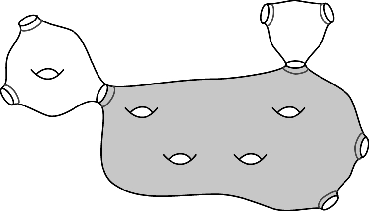
 g=4
 b=4
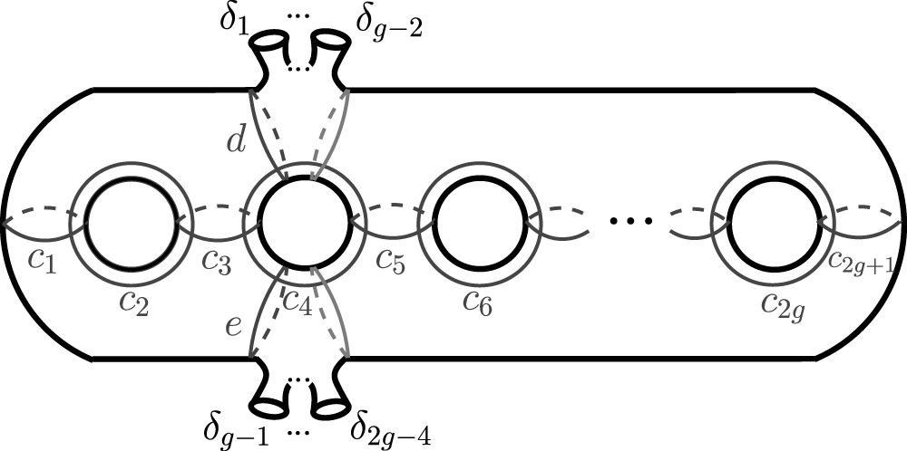
 ci,d,e
 Σg2g−4
 δj
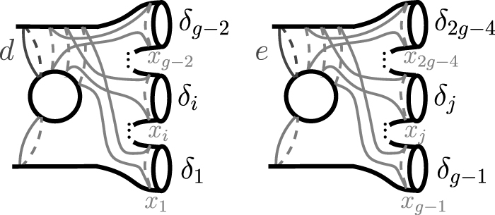
 xj
 Σg2g−4
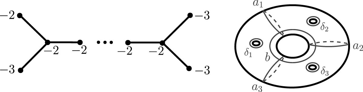
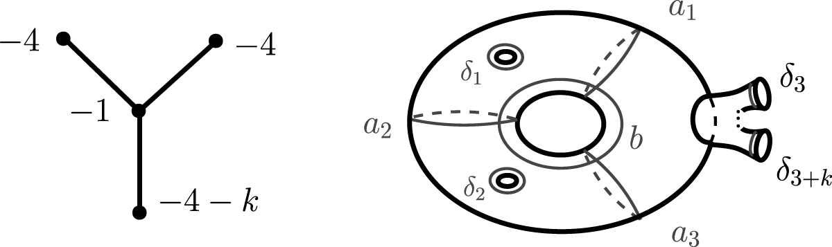
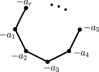
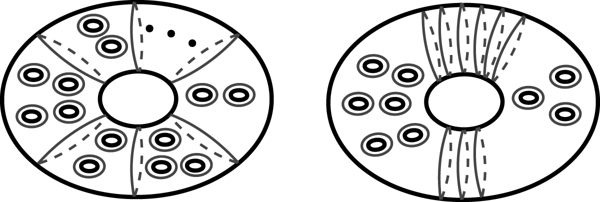
 −ai
 ai−2
 ai=2
 a1=4,a2=6,a3=4,a4=5,a5=4,…
 a1=8,a2=a3=2,a4=5,a5=a6=⋯=a9=2


