



1. Introduction
The secondary driver was first proposed by Henshall (Reference Henshall1956) and evaluated experimentally by Stalker & Plumb (Reference Stalker and Plumb1968). It is normally used in expansion tubes to increase the shock strength through the test gas for high-enthalpy, superorbital conditions, and consists of an additional section of helium between the primary diaphragm and the shock tube. The theoretical principles of this mode of operation are well established (Morgan & Stalker Reference Morgan and Stalker1991; Morgan Reference Morgan, Ben-Dor, Igra and Elperin2001a ); however, its effective implementation in an expansion tube is non-trivial for two reasons: firstly, the device increases the already large number of facility variables which must each be configured to achieve the desired test condition; secondly, for certain parts of the facility operating envelope, it can introduce complex secondary wave processes (Gildfind et al. Reference Gildfind, Morgan, McGilvray and Jacobs2014).
This study was motivated by recent experimentation with scramjet flow conditions using the The University of Queensland’s X2 expansion tube (Gildfind et al. Reference Gildfind, Morgan, McGilvray and Jacobs2014). Expansion tube operation of scramjet flow conditions typically leads to a drop in sound speed across the driver/test gas interface (referred to as ‘under-tailored’ operation), which has been shown to promote transmission of driver disturbances to the test gas, leading to unacceptable noise levels in the final test flow (Paull & Stalker Reference Paull and Stalker1992). For these conditions a secondary driver has previously been suggested (Morgan & Stalker Reference Morgan and Stalker1991) as a means to ensure that sound speed increases across this interface (‘over-tailored’ operation).
However, in the X2 scramjet flow condition experiments, it was found that traditional analytical techniques did not accurately predict the actual facility response for this configuration. This was attributed to close coupling of driver wave processes; however, the broader implications of this issue were not explored. The present study now examines this issue from an operational perspective, in order to establish exactly how the secondary driver affects facility response across its entire operating envelope. In doing so, the aim is to explain the unpredictable behaviour, and to develop robust guidelines for using this operating mode.
The study begins with an ideal gas analysis of a generic expansion tube across its entire practical operating envelope, using air as the test gas. A specific study of UQ’s medium-sized X2 expansion tube is then performed, using equilibrium chemistry, in order compare the purely theoretical predictions with an actual facility. Numerical and experimental studies of X2 are finally used to establish which parts of the operating envelope can be accurately modelled with traditional analytical techniques, which parts require higher-fidelity numerical simulation, and the reasons for these differences are explained. Based on this wide-ranging study, general conclusions are drawn about how the response of a secondary driver changes across the entire operating envelope of an expansion tube facility, thereby providing a comprehensive and unambiguous guide to its effective implementation for expansion tubes in general.
2. Free-piston-driven expansion tubes
Free-piston-driven expansion tubes can produce the highest enthalpy and highest total pressure test flows of any type of wind tunnel test facility currently in operation. This potential has already been widely utilised for simulation of superorbital planetary entry flows up to
 $20~\text{km}~\text{s}^{-1}$
(for example, Morgan & Stalker Reference Morgan and Stalker1991; Neely & Morgan Reference Neely and Morgan1994; Jacobs Reference Jacobs2011; Capra & Morgan Reference Capra and Morgan2012; Eichmann Reference Eichmann2012; Porat et al.
Reference Porat, Zander, Morgan and McIntyre2013; Sheikh et al.
Reference Sheikh, Jacobs, Laux, Morgan and McIntyre2013; James et al.
Reference James, Gildfind, Morgan and McIntyre2014), and their multi-gigapascal total pressure capability also makes these facilities uniquely capable of simulating the high-Mach-number flight conditions associated with scramjet access-to-space (McGilvray, Morgan & Jacobs Reference McGilvray, Morgan and Jacobs2010; Gildfind, Sancho & Morgan Reference Gildfind, Sancho and Morgan2013; Gildfind et al.
Reference Gildfind, Morgan, McGilvray and Jacobs2014). Both applications provide the context for this current paper.
Figure 1 shows the configuration of a basic free-piston-driven expansion tube, along with an idealised
 $x{-}t$
diagram of the flow processes which occur during its operation. Compressed air from a high-pressure reservoir accelerates a massive piston down the driver/compression tube, which is sealed from the driven tube by a steel primary diaphragm. Between the piston and the diaphragm is a light driver gas such as helium, or a mixture of helium and argon. The piston accelerates across most of its stroke, reaching speeds of between 100 and
 $300~\text{m}~\text{s}^{-1}$
, and accumulates significant kinetic energy. Towards the end of the piston stroke, the driver gas compression ratio begins to rise rapidly. The piston transfers its kinetic energy to the driver gas, increasing the driver gas pressure and temperature until the steel diaphragm ruptures, whereupon the driver gas expands into the driven tube.
Idealised distance–time (
 $x{-}t$
) diagram showing flow processes for a basic expansion tube: s
 $=$
shock; rs
 $=$
reflected shock; cs
 $=$
contact surface; sx
 $=$
steady expansion; usx
 $=$
unsteady expansion;
 $u+a=\text{reflected}$
characteristic.

The driven tube has a smaller diameter and runs continuously from the primary diaphragm through to the test section. This tube can be partitioned into a series of shorter sections using thin (typically) Mylar film diaphragms. Each section can be operated with gases of different composition and initial fill pressure. In basic expansion tube mode, the driven tube is partitioned with a single diaphragm, referred to as the secondary diaphragm in figure 1. The test gas is located between the primary and secondary diaphragms, in the section referred to as the shock tube. The section of tube downstream of the secondary diaphragm – the acceleration tube – runs through to the test section, and is initially at very low pressure. Experiments take place at the exit of this tube.
The driver gas pressure and temperature are, respectively, tens of megapascals and thousands of Kelvin when the primary diaphragm ruptures. The expanding driver gas drives a strong shock through the test gas, compressing it and accelerating it towards the test section. When the hot and high-pressure test gas impacts the thin secondary diaphragm, its speed is typically between 1 and
 $6~\text{km}~\text{s}^{-1}$
. The secondary diaphragm disintegrates, exposing the test gas to the low pressure (of the order of 100–102 Pa) of the downstream acceleration tube. This sudden drop in pressure causes the test gas to undergo a strong unsteady expansion, accelerating it to the final test flow velocity.
When a supersonic flow undergoes an unsteady expansion, both its total pressure and total temperature increase. Since the test gas is not stagnated during this process, expansion tubes do not suffer from the total pressure and temperature limits of facilities which do stagnate the test gas, such as reflected shock tunnels (RSTs) (Bakos & Erdos Reference Bakos and Erdos1995), and dissociation and radiative losses are similarly avoided (Bakos, Morgan & Tamagno Reference Bakos, Morgan and Tamagno1992; Morgan Reference Morgan, Ben-Dor, Igra and Elperin2001a ). However, since only part of the test gas can be expanded to the required test condition, test times are short in comparison to RST facilities of equivalent size (Morgan Reference Morgan, Ben-Dor, Igra and Elperin2001a ).
Inspecting regions 1, 2 and 5–7 in figure 1, when the secondary diaphragm is ruptured, the region 2 gas undergoes an unsteady expansion which is bounded by the initial fill pressure in the acceleration tube,
 $p_{5}$
. Ignoring processes upstream of the shock tube for now, and making ideal gas assumptions, it follows that any given test flow condition (i.e. region 7) will be defined by a single pair of shock speeds through the shock and acceleration tubes, and the ratio of fill pressures
 $p_{5}/p_{1}$
; the static pressure of the final test flow will then depend on the initial shock tube fill pressure,
 $p_{1}$
. The fundamental purpose of the driver is therefore to generate a shock of the required strength, through a test gas at the required
 $p_{1}$
. If an appropriate
 $p_{5}$
is set, then the test gas will expand to the required condition. These general trends are qualitatively observed even when real gas effects become important.
In practice, many other aspects of the facility configuration also affect the eventual performance which can be achieved. For example, the effect of boundary layers on the core flow size and final test flow velocity, which was first characterised by Duff (Reference Duff1959) and later quantified by Mirels (Reference Mirels1963a ,Reference Mirels b ), is more significant for relatively slender tubes and lower density gases. The effective ‘holding time’ of the free-piston driver – i.e. the amount of time at which driver pressure is held at relatively high levels – can also significantly impact test flow properties if it is insufficient (Gildfind et al. Reference Gildfind, Morgan, McGilvray, Jacobs, Stalker and Eichmann2011). However, while factors such as these can potentially impose significant limitations on the performance of a facility, they are secondary in nature and can often be accounted for with careful tuning of the given facility at hand. On the other hand, the factor which most affects the fundamental performance of a facility is the state of the driver gas – in terms of sound speed and pressure – when the primary diaphragm ruptures.
2.1. Expansion tube driver requirements
Morgan & Stalker (Reference Morgan and Stalker1991) and Morgan (Reference Morgan, Ben-Dor, Igra and Elperin2001a
,Reference Morgan, Ben-Dor, Igra and Elperin
b
) have extensively investigated the driver requirements for shock tunnel and expansion tube operation, particularly for expansion tubes operating at superorbital flight conditions. Referring to figure 1, and noting that across the interface the speed of the expanded driver gas,
 $u_{3}$
, equals the post-shock test gas velocity,
 $u_{2}$
, Morgan (Reference Morgan, Ben-Dor, Igra and Elperin2001b
) normalised this velocity by the unexpanded driver gas sound speed,
 $a_{4}$
:
 $$\begin{eqnarray}Ma_{3}^{\ast }=u_{3}/a_{4}.\end{eqnarray}$$
 $Ma_{3}^{\ast }$
is termed the ‘driver equivalent Mach number’ (Morgan Reference Morgan, Ben-Dor, Igra and Elperin2001b
). By using velocity instead of driven shock Mach number, and by non-dimensionalising
 $u_{3}$
in terms of
 $a_{4}$
, the pressure ratio
 $p_{3}/p_{4}$
becomes independent of the driven gas composition (Morgan Reference Morgan, Ben-Dor, Igra and Elperin2001b
). Using a perfect gas analysis, where
 ${\it\gamma}$
is the ratio of specific heats, Morgan arrived at the following driver relation:
 $$\begin{eqnarray}\frac{p_{3}}{p_{4}}=\left[F_{1}-Ma_{3}^{\ast }\frac{({\it\gamma}_{4}-1)}{2}\right]^{2{\it\gamma}_{4}/({\it\gamma}_{4}-1)},\end{eqnarray}$$
where:
 $$\begin{eqnarray}F_{1}=\left\{\left[1+\frac{{\it\gamma}_{4}-1}{2}Ma_{4^{\prime \prime }}^{2}\right]^{-0.5}\left[1+\frac{{\it\gamma}_{4}-1}{2}Ma_{4^{\prime \prime }}\right]\right\}.\end{eqnarray}$$
 $F_{1}$
is a parameter which accounts for the geometric transition from the driver to driven tubes. In figure 1,
 $Ma_{4^{\prime \prime }}=1$
; the flow is choked since there is a significant area change, and this is also the highest performance arrangement at the tube transition (Morgan Reference Morgan, Ben-Dor, Igra and Elperin2001b
).
Equation (2.2) indicates the extent to which the driver gas must expand, from its initial pressure,
 $p_{4}$
, to
 $p_{3}$
(which is equal to the post-shock pressure, i.e.
 $p_{3}=p_{2}$
), to achieve a given
 $Ma_{3}^{\ast }$
, and is plotted in figure 2. These results are for a facility with an area change at the driver, therefore
 $Ma_{4^{\prime \prime }}=1$
. Morgan (Reference Morgan, Ben-Dor, Igra and Elperin2001b
) notes that the maximum possible
 $Ma_{3}^{\ast }$
is achieved in the limiting case, when the driver gas expands to zero pressure; i.e.
 $p_{3}/p_{4}=0$
. Solving for
 $Ma_{3}^{\ast }$
:
 $$\begin{eqnarray}Ma_{3}^{\ast }=2F_{1}/({\it\gamma}_{4}-1).\end{eqnarray}$$


For
 ${\it\gamma}_{4}=5/3$
and
 $Ma_{4^{\prime \prime }}=1$
, equation (2.4) gives
 $Ma_{3}^{\ast }=3.46$
; for helium at room temperature (300 K) this corresponds to
 $u_{3}=3536~\text{m}~\text{s}^{-1}$
; for helium at 5000 K, which represents a free-piston driver operating at a high compression ratio,
 $u_{3}=11\,150~\text{m}~\text{s}^{-1}$
. However, observing figure 2, it can be seen that the ratio
 $p_{3}/p_{4}$
drops rapidly for
 $Ma_{3}^{\ast }>2$
; Morgan (Reference Morgan, Ben-Dor, Igra and Elperin2001a
) notes that pressure recovery becomes too low beyond this point; the implications are test gas densities which are impractically low, and test flows which become overwhelmed by viscous effects (Mirels Reference Mirels1963a
,Reference Mirels
b
).
A practical limit of
 $Ma_{3}^{\ast }=2$
corresponds to intermediate test gas flow velocities (region 2 in figure 1) of
 $2038~\text{m}~\text{s}^{-1}$
and
 $6445~\text{m}~\text{s}^{-1}$
for a helium driver at 300 K and 5000 K, respectively; this, in turn, sets a limit on final test flow velocity as well, since there are limits to the enthalpy and total pressure increases which are possible across the unsteady expansion (Morgan (Reference Morgan, Ben-Dor, Igra and Elperin2001a
) quoting Lucasiewicz (Reference Lucasiewicz1973) notes that up to a doubling of flow velocity can typically be achieved across an unsteady expansion). While these calculations are perfect gas estimates, they nevertheless provide an indication of the fundamental limitations of this type of driver arrangement.
2.2. Expansion tube operation with a shock-heated secondary driver
Figure 3 shows an idealised
 $x{-}t$
diagram of the flow processes which occur for an expansion tube operating with a secondary driver. To enable this mode, a second thin Mylar diaphragm is used to locate a volume of helium gas between the primary diaphragm and the test gas. This is termed the secondary diaphragm; the downstream diaphragm separating the test and accelerator gases becomes the tertiary diaphragm.
Idealised distance–time (
 $x{-}t$
) diagram showing flow processes for an expansion tube with secondary driver and unsteady expansion at secondary diaphragm: s
 $=$
shock; rs
 $=$
reflected shock; cs
 $=$
contact surface; sx
 $=$
steady expansion; usx
 $=$
unsteady expansion;
 $u+a=\text{reflected}$
characteristic.

This additional tube section is referred to as a secondary driver because it becomes the driver for the actual test gas (the combination of primary and secondary drivers is then referred to as a ‘compound driver’). If this section of tube has a sufficiently low initial fill pressure, shock processing of its helium can raise its temperature,
 $T_{sd2}$
, and therefore sound speed,
 $a_{sd2}$
, far above the equivalent values of the expanded primary driver gas,
 $T_{sd3}$
and
 $a_{sd3}$
. When
 $a_{sd2}>a_{sd3}$
, the secondary driver is said to be ‘over-tailored’. This can result in the secondary driver generating a stronger shock through the test gas than the primary driver would be able to by itself; this performance increasing potential was the motivation for initial work with these devices, and has previously been analysed and confirmed experimentally (Henshall Reference Henshall1956; Stalker & Plumb Reference Stalker and Plumb1968; Morgan & Stalker Reference Morgan and Stalker1991; Neely & Morgan Reference Neely and Morgan1994; Morgan Reference Morgan1997, Reference Morgan, Ben-Dor, Igra and Elperin2001a
).
Figure 4 (from Morgan Reference Morgan, Ben-Dor, Igra and Elperin2001a
) compares the pressure recovery,
 $p_{3}/p_{4}$
, as a function of
 $Ma$
, for three different driver options. Taking into account practical limitations of facility operation, Morgan (Reference Morgan, Ben-Dor, Igra and Elperin2001a
) determined that a compound driver can extend the maximum practical driver equivalent Mach number from 2 to 4. This therefore opens up the possibilities of simulating flight enthalpies to
 $20\,000~\text{m}~\text{s}^{-1}$
and beyond – for example, return from missions to the Far Solar System (entry to Earth’s atmosphere at speeds up to
 $16\,000~\text{m}~\text{s}^{-1}$
), or entry to the gas giants (atmospheric entry at speeds exceeding
 $20\,000~\text{m}~\text{s}^{-1}$
) – and is why this operating regime is referred to as ‘superorbital’ expansion tube operation. This superorbital mode was first demonstrated by Morgan & Stalker (Reference Morgan and Stalker1991), who achieved shock speeds up to
 $18.7~\text{km}~\text{s}^{-1}$
; Neely & Morgan (Reference Neely and Morgan1994) further developed the concept, with test flows up to
 $13~\text{km}~\text{s}^{-1}$
.
Pressure recovery,
 $p_{3}/p_{4}$
, as a function of driver equivalent Mach number,
 $Ma_{3}^{\ast }$
, for different driver options (adapted from Morgan Reference Morgan, Ben-Dor, Igra and Elperin2001a
).

2.3. Secondary driver as acoustic buffer
The first experiments with expansion tubes, which took place in the 1960s and 1970s in the United States, had in common the disappointing feature that most test flows had unacceptable levels of noise (Jones Reference Jones1965; Norfleet, Lacey & Whitfield Reference Norfleet, Lacey and Whitfield1965; Spurk Reference Spurk1965; Miller Reference Miller1977; Miller & Jones Reference Miller, Jones, Archer and Milton1983). Miller (Reference Miller1977), who conducted the first extensive expansion tube study with the NASA Langley Expansion Tube/Tunnel, would later note that only a very narrow range of suitably steady test flows could be achieved (Miller & Jones Reference Miller, Jones, Archer and Milton1983).
In the 1980s, The University of Queensland (UQ) was contracted by NASA Langley to investigate expansion tube operation with a free-piston driver (Stalker Reference Stalker and Kim1990). Paull, Stalker & Stringer (Reference Paull, Stalker and Stringer1988) undertook a systematic study with the new TQ facility to identify the reasons for the test flow unsteadiness which had been observed in the earlier expansion tube experiments. Paull & Stalker (Reference Paull and Stalker1992) would eventually categorise test flows as being either high enthalpy or low enthalpy, and determined that test flow noise was associated with the low-enthalpy flows.
Paull & Stalker (Reference Paull and Stalker1992) analysed the effect of the unsteady expansion on noise in the test gas, and found that the sound speed drop through the unsteady expansion had the effect of focusing the frequency components of lateral acoustic waves into a narrow bandwidth of frequencies, which would later appear as strong disturbances in the test flow. While this phenomenon was present for both high- and low-enthalpy conditions, the high-enthalpy test flows were relatively free from disturbances because the test gas had low levels of noise prior to the unsteady expansion. The critical next step was to determine that, for high-enthalpy conditions, the test gas was relatively free of noise because the sound speed of the shock-processed test gas,
 $a_{2}$
in figure 1, was higher than the sound speed of the expanded driver gas,
 $a_{3}$
(Paull & Stalker Reference Paull and Stalker1992).
The driver gas expansion through the driver area change and primary diaphragm is a fundamental source of lateral wave disturbances (radial disturbances in an axisymmetric facility) (Jacobs Reference Jacobs1994). Jacobs (Reference Jacobs1994) performed numerical simulations of the NASA Langley facility and showed that these radial disturbances could indeed propagate into the test gas. The principal conclusion from the Paull & Stalker (Reference Paull and Stalker1992) work was that it was necessary to operate an expansion tube in an over-tailored configuration (
 $a_{2}/a_{3}>1.25$
was suggested) in order to achieve an ‘acoustic buffer’ against driver gas disturbances.
The acoustic buffer requirement clearly has implications for expansion tube operation at lower enthalpies; Morgan (Reference Morgan, Ben-Dor, Igra and Elperin2001a
) determined that operating a basic expansion tube with
 $a_{2}/a_{3}>1.25$
would require
 $Ma_{3}^{\ast }>1.4$
. While it becomes possible to use alternative facilities, such as RSTs, to simulate these low-enthalpy test flows, there are some applications where the total pressure requirement far exceeds what other facilities can deliver. For example, high-Mach-number scramjet test flows (
 $3{-}5~\text{km}~\text{s}^{-1}$
) can have gigapascal total pressure requirements (Gildfind et al.
Reference Gildfind, Morgan, McGilvray and Jacobs2014); however, RSTs are structurally limited to total pressures of between 150 and 300 MPa (Bakos & Erdos Reference Bakos and Erdos1995).
Noting that over-tailored operation is a fundamental aspect of secondary driver operation, Morgan & Stalker (Reference Morgan and Stalker1991) proposed that for low-enthalpy conditions the acoustic buffer function could be met with the secondary driver, thereby, in theory, restoring the useful operational envelope of expansion tubes back to the initial predictions of Trimpi (Reference Trimpi1962). Thus, these initial years of expansion tube research at UQ led to the discovery of the mechanism responsible for the disappointingly noisy test flows in earlier studies (Paull et al. Reference Paull, Stalker and Stringer1988; Paull & Stalker Reference Paull and Stalker1992), furthermore, the shock-heated secondary driver was introduced as a means to boost performance at superorbital conditions, and was simultaneously identified as a solution to the test flow noise problem (Morgan & Stalker Reference Morgan and Stalker1991; Morgan Reference Morgan, Ben-Dor, Igra and Elperin2001a ).
3. Theoretical performance of an expansion tube with secondary driver
As noted in § 2, there are two fundamental processes associated with producing an expansion tube test flow. Firstly, a test gas of defined composition and initial fill pressure,
 $p_{1}$
, must be shock-processed to the required intermediate speed,
 $u_{2}$
, and temperature,
 $T_{2}$
. Secondly, a low acceleration tube fill pressure,
 $p_{5}$
, is selected which will bound the unsteady expansion so that the shock-processed test gas expands to the required test flow velocity,
 $u_{7}$
, temperature,
 $T_{7}$
, and corresponding pressure,
 $p_{7}$
. The performance of an expansion tube driver can be assessed during the first stage alone; i.e. measured in terms of the strength of shock which it can generate through the test gas.
In this section the influence of a secondary driver on expansion tube performance is thus assessed in terms of the pressure ratio which is achieved across the test gas shock, i.e.
 $p_{2}/p_{1}$
. The purpose is not simply to determine the region of maximum performance gain, but to obtain an understanding of how the secondary driver influences performance across the entire facility operating envelope. This becomes important when a secondary driver is used as an acoustic buffer for low-enthalpy flow conditions, since this changes its mode of operation in comparison to superorbital configurations.
Ideal gas properties are assumed, which allows the facility operating envelope to be defined in terms of two initial fill pressure ratios:
-
(a) The ratio between primary driver gas pressure at diaphragm rupture and test gas fill pressure,
 $p_{4}/p_{1}$
.
-
(b) The ratio between secondary driver and test gas fill pressures,
$p_{sd1}/p_{1}$
.


The ratio
 $p_{4}/p_{1}$
can also be used to calculate the test gas shock strength when a secondary driver is not used, and therefore provides a basis for comparison.
In this analysis the test gas is assumed to be air, and the primary and secondary driver gases are assumed to be helium. All gases are assumed to be at an initial temperature of 300 K; the primary driver gas then undergoes an isentropic compression to a temperature based on the driver gas compression ratio,
 ${\it\lambda}$
(also specified). Trimpi’s (Reference Trimpi1962) expansion tube analytical framework has been adapted to include an optional secondary driver. The driver is assumed to have a simple area change, which expands the driver gas to sonic conditions at the opening to the driver tube.
A requirement of the analytical solution approach is to establish a finite set of longitudinal wave processes for consideration during the solution process. Three typical expansion tube operating modes are considered, based on the preceding discussion:
-
(a) Figure 1 shows the basic expansion tube operating mode. The test gas is shock-processed, and then undergoes an unsteady expansion into the low-pressure acceleration tube when it ruptures the secondary diaphragm.
-
(b) Figure 3 shows an expansion tube with secondary driver. In this configuration the test gas is initially at low density relative to the secondary driver gas, and the shock-processed helium undergoes an unsteady expansion when it ruptures the secondary diaphragm. The shock-processed air then undergoes an unsteady expansion when it arrives at, and ruptures, the tertiary diaphragm. This is the assumed operating mode of previous secondary driver studies targeting superorbital expansion tube operation (Morgan & Stalker Reference Morgan and Stalker1991; Neely & Morgan Reference Neely and Morgan1994).
-
(c) Figure 5 also shows an expansion tube with secondary driver. The difference compared to figure 3 is that the test gas initially has sufficiently high density, compared to the secondary driver gas, that the shock-processed secondary driver gas must slow when it impacts the test gas. This deceleration and corresponding compression occur due to a reflected shock originating at the secondary diaphragm. The remaining downstream flow processes are otherwise similar to figure 3.
Idealised distance–time (
 $x{-}t$
) diagram showing flow processes for an expansion tube with secondary driver and reflected shock at secondary diaphragm: s
 $=$
shock; rs
 $=$
reflected shock; cs
 $=$
contact surface; sx
 $=$
steady expansion; usx
 $=$
unsteady expansion;
 $u+a=\text{reflected}$
characteristic.

Appendix A details the steps involved in solving for the test flow properties, given an initial pair of pressure ratios,
 $p_{4}/p_{1}$
and
 $p_{sd1}/p_{1}$
. The results of the analysis are shown in figure 6. Figure 6(a) shows the computed pressure ratio across the test gas shock,
 $p_{2}/p_{1}$
, for an expansion tube operating both with (shaded surface) and without (white surface) a secondary driver. The driver compression ratio is
 ${\it\lambda}=1$
for both solutions (i.e. no compressive heating of the driver gas).
Influence of a helium secondary driver on pressure ratio across test gas shock wave, for air test gas and helium primary driver; (a), (c) and (e) show
 $p_{2}/p_{1}$
, with and without secondary driver, for
 ${\it\lambda}=1$
, 10 and 100, respectively; (b), (d) and (f) show the ratio between the two shock-processed test gas pressure ratios, with and without secondary driver, also for
 ${\it\lambda}=1$
, 10 and 100, respectively.

It can be seen that the white surface plot in figure 6(a) is invariant with
 $p_{sd1}/p_{1}$
since it considers the basic expansion tube without secondary driver. However, it can be seen that the shaded plot varies significantly with this ratio. There is a clear region of operation where the secondary driver theoretically imparts a performance increase. On the log–log scale shown, this region is delineated by two approximately straight boundaries:
-
(a) The dashed black curve in figure 6(a) represents the tailored condition in figure 3 where the sound speed of the expanded primary driver gas,
$a_{sd3}$
, is equal to the sound speed of the shock-processed secondary driver gas,
$a_{sd2}$
. Noting (3.1), and that the primary driver sound speed,
$a_{4}$
, is constant for all of figure 6(a), then tailored operation corresponds to a single secondary driver shock speed, and therefore a fixed pressure ratio,
$p_{4}/p_{sd1}$
; this explains why the dashed curve is straight: (3.1)
$$\begin{eqnarray}\frac{p_{4}}{p_{sd1}}=\frac{p_{4}}{p_{1}}\cdot \frac{p_{1}}{p_{sd1}}.\end{eqnarray}$$
Considering each point on the dashed curve, at higher ratios of
$p_{sd1}/p_{1}$
the condition
$a_{sd2}>a_{sd3}$
arises, and the secondary driver is said to be ‘over-tailored’ with respect to the primary driver gas. This is the fundamental operating regime which allows the secondary driver gas to achieve a stronger shock than the primary driver gas alone (Morgan Reference Morgan, Ben-Dor, Igra and Elperin2001a
), and corresponds to a performance increase relative to the basic expansion tube. Conversely, at lower ratios of
$p_{sd1}/p_{1}$
the secondary driver is under-tailored, and the performance is reduced in comparison to the basic expansion tube. -
(b) A solid black diagonal line is shown in figure 6(a); this marks the beginning of the region of operation where a reflected shock forms upon rupture of the secondary diaphragm (i.e. the case shown in figure 5), and
$p_{2}/p_{1}$
is seen to reduce compared to the basic expansion tube. For each point on the solid curve, a smaller ratio of
$p_{sd1}/p_{1}$
will result in a performance reduction compared to the basic expansion tube. This operating mode is examined in more detail in § 3.1.


The shaded surface in figure 6(b) shows the local ratio between the two surfaces in figure 6(a), again for
 ${\it\lambda}=1$
; this has been calculated by dividing each local pressure ratio for operation with a secondary driver (from the shaded surface in figure 6(a), and denoted here as
 $p_{2,sd}$
) by the corresponding pressure ratio for operation without a secondary driver (from the white surface in figure 6(a), and denoted
 $p_{2}$
). The white surface in figure 6(b) shows the ratio
 $p_{2,sd}/p_{2}=1$
; anywhere that the shaded surface exceeds this level, the secondary driver theoretically provides a performance increase. The dashed and solid curves once more delineate this region of performance increase; the dashed curve defines the boundary between over-tailored and under-tailored operation; the solid curve defines the threshold where the unsteady expansion is replaced by a reflected shock at the secondary diaphragm.
The analysis of figure 6(a,b) is repeated for
 ${\it\lambda}=10$
and
 ${\it\lambda}=100$
in 6(c,d) and 6(e,f), respectively. Considering the entire set of plots, four features are evident:
-
(a) The shapes of each surface, and the delineating dashed and solid boundaries, are all qualitatively the same.
-
(b) With increased driver compression ratio,
${\it\lambda}$
, the absolute pressure ratio achieved by the driver, both with and without secondary driver, increases. -
(c) Within the range of fill pressure ratios considered, the relative performance increase (i.e. figure 6 b,d,f) achieved with the secondary driver diminishes with increased
${\it\lambda}$
. -
(d) There is a small region in figure 6(c–f) where under-tailored operation, combined with a reflected shock at the secondary diaphragm, theoretically results in a marginal increase in performance compared to the basic expansion tube (this is most evident in figure 6 f).


3.1. Reflected shock at the secondary diaphragm
An important feature in figure 6 is that although the secondary driver can be configured for over-tailored operation across a large part of the performance envelope, this performance increase is lost if a reflected shock arises at the secondary diaphragm. While it will be later shown that this becomes a fundamental feature of secondary driver operation at lower enthalpies, where the device is used as an acoustic buffer, in this section the conditions to produce a reflected shock are first examined.
Whether or not a reflected shock arises at the secondary diaphragm depends primarily on the ratio of initial fill pressures in the secondary driver and shock tubes (
 $p_{sd1}$
and
 $p_{1}$
, respectively), and to a lesser extent on the strength of the resulting shock in the shock tube. For
 $p_{1}\ll p_{sd1}$
, an unsteady expansion will occur; if
 $p_{1}$
is increased, eventually a point will be reached where the unsteady expansion has zero strength; if
 $p_{1}$
is further increased, a reflected shock wave will form. The weakest reflected shock will be a Mach wave, and will produce negligible pressure rise, and negligible deceleration, of the region
 $sd2$
flow; for this case
 $u_{sd2}=u_{3}$
and
 $p_{sd2}=p_{3}$
. If ideal gas assumptions are made, the density ratio associated with this condition,
 ${\it\rho}_{sd1}/{\it\rho}_{1}$
, can be solved as a function of test gas shock strength, expressed in terms of Mach number
 $Ma_{s,1}$
. Section A.3 details the procedure to solve for the reflected Mach wave case; the results are shown in figure 7.
Effect of secondary driver/test gas fill density ratio,
 ${\it\rho}_{sd1}/{\it\rho}_{1}$
, on post-diaphragm rupture flow processes. Secondary driver is helium; test gas is air.

Figure 7 shows two solutions for the reflected Mach wave case. The curve denoted ‘Solution 1’ is the only physical solution. It can be seen that, except for weak shocks, the ratio
 ${\it\rho}_{sd1}/{\it\rho}_{1}\approx 0.9$
indicates the density ratio below which a reflected shock will form in the secondary driver gas. For
 ${\it\rho}_{sd1}/{\it\rho}_{1}>0.9$
, the secondary driver gas is sufficiently dense that it will undergo an unsteady expansion into the test gas for all test gas shock speeds.
‘Solution 2’ in figure 7 represents the shock Mach number which the secondary driver will drive through the test gas simply by virtue of its high initial fill pressure; i.e. with no initial velocity, and independent of the upstream driver. It is a non-physical solution, since this expansion process must occur through an expansion wave, not a Mach wave. The correct solution is given by (3.2), which is the basic shock tube equation (equation (7.94) from Anderson Reference Anderson1990), and is the dashed curve shown in figure 7. The two solutions are coincidentally equal for
 $Ma_{s,1}=1$
, for which the driven shock through the test gas is a Mach wave with no associated pressure rise; the two curves diverge for
 $Ma_{s,1}>1$
, since only the shock tube equation is physically correct.
 $$\begin{eqnarray}\frac{p_{sd1}}{p_{1}}=\frac{p_{2}}{p_{1}}\left\{1-\frac{({\it\gamma}_{sd}-1)\left({\displaystyle \frac{a_{1}}{a_{sd1}}}\right)\left({\displaystyle \frac{p_{2}}{p_{1}}}-1\right)}{\sqrt{2{\it\gamma}_{1}\left[2{\it\gamma}_{1}+({\it\gamma}_{1}+1)\left({\displaystyle \frac{p_{2}}{p_{1}}}-1\right)\right]}}\right\}^{-2{\it\gamma}_{sd}/({\it\gamma}_{sd}-1)}.\end{eqnarray}$$
For an air test gas, the result observed in figure 7 effectively limits the use of a secondary driver as a performance increasing device to superorbital conditions only. This limitation will be less restrictive for lighter test gases.
4. X2 driver performance envelope
In this section the performance envelope of the X2 expansion tube is examined using the facility’s high-performance 100 % helium tuned-driver condition. This condition is described in Gildfind, James & Morgan (Reference Gildfind, James and Morgan2015), and summarised in table 1. A schematic of the X2 facility is shown in figure 8, and a detailed overview of the facility is provided in Gildfind et al. (Reference Gildfind, Morgan, McGilvray and Jacobs2014). The analysis of Gildfind et al. (Reference Gildfind, James and Morgan2015) determined that reasonably accurate driven shock speed estimates could be obtained analytically by assuming a constant driver temperature and pressure of
 $\overline{T}_{4}=2903~\text{K}$
and
 $\overline{p}_{4}=27.4~\text{MPa}$
, respectively, and treating the driver gas as ideal.
The University of Queensland’s X2 expansion tube facility (to scale). Supporting carriage work, pressure manifold and associated hardware are not shown.

X2 10.5 kg piston-tuned driver condition, with effective
 $\overline{p}_{4}$
and
 $\overline{T}_{4}$
of 27.4 MPa and 2903 K, respectively (Gildfind et al.
Reference Gildfind, James and Morgan2015); driver gas composition is by partial pressure; diaphragms are fabricated from cold rolled steel.

The discrepancy between analytical calculations and experimentally measured shock speeds was less than 3 % for shock speeds into a helium driver gas between approximately 4 and
 $9~\text{km}~\text{s}^{-1}$
; another
 $5~\text{km}~\text{s}^{-1}$
shock speed through air was predicted to within 3.6 % (using equilibrium gas assumptions for the air). Since the present analysis is focused on shock speeds through a helium secondary driver, the analytical values derived in Gildfind et al. (Reference Gildfind, James and Morgan2015) are considered a good basis for such a parametric study.
Using effective driver gas properties from table 1, an iterative analytical routine was established to predict the shock speed through an air test gas for X2 expansion tube operation with and without a secondary driver. Flow processes were assumed to follow those shown in figures 1, 3 and 5. For this driver condition, an orifice plate is located at the driver area change; this was modelled in accordance with the methodology detailed in Gildfind et al. (Reference Gildfind, James and Morgan2015). Ideal gas properties were assumed for primary driver and secondary driver helium gases; equilibrium gas properties were used for the air test gas, and were calculated using CEA (Chemical Equilibrium with Applications) (Gordon & McBride Reference Gordon and McBride1994). The basic methodology to calculate equilibrium shock speeds through the test gas was as follows:
-
(a) A matrix of combinations of helium secondary driver fill pressure,
$p_{sd1}$
, and air test gas fill pressure,
$p_{1}$
, was established. Both
$p_{sd1}$
and
$p_{1}$
were varied between 102 and
$10^{6}~\text{Pa}$
, and incremented with equal-sized steps on a log scale. -
(b) The shock speed through the secondary driver was calculated in accordance with § A.2, providing the post-shock properties in region
$sd2$
(figure 3). -
(c) For each
$p_{1}$
, CEA was used to calculate post-shock flow properties through air, across shock speeds ranging from 400 to
$11\,000~\text{m}~\text{s}^{-1}$
, incremented by
$50~\text{m}~\text{s}^{-1}$
, and covering the likely range of shock speeds through the test gas. These results were recorded as a look-up-table for subsequent calculations; this would then provide equilibrium curves of
$p_{2}$
versus
$u_{2}$
for each
$p_{1}$
. -
(d) Test gas shock speeds for each
$p_{sd1}$
were calculated for both unsteady expansion (figure 3) and reflected shock (figure 5) wave processes at the secondary diaphragm. For the unsteady expansion case, the region
$sd2$
gas was incrementally expanded to a pressure approaching zero, and the corresponding velocity calculated at each point; for the reflected shock case, the region
$sd2$
gas was compressed by a reflected shock to a velocity approaching zero, and the corresponding pressure calculated; both calculation procedures were based on the methodology detailed in § A.2. The outputs of this calculation were curves of
$p_{sd2}$
versus
$u_{sd2}$
for both unsteady expansion and reflected shock cases. -
(e) At the final step, for each
$p_{1}$
, the intersections between the equilibrium air
$p_{2}$
versus
$u_{2}$
curve and the two
$p_{sd2}$
versus
$u_{sd2}$
curves were calculated. The unsteady expansion solution was considered to be correct if both
$p_{sd2}>p_{3}$
and
$u_{sd2}<u_{3}$
; otherwise the reflected shock solution was used, where
$p_{sd2}<p_{3}$
and
$u_{sd2}>u_{3}$
. The type of solution was also recorded for each
$p_{1}$
. -
(f) A similar procedure was also used to calculate the test gas shock speed for a basic expansion tube without a secondary driver. In this case, the region
$4^{\prime \prime }$
driver gas undergoes an unsteady expansion to the test gas velocity in accordance with § A.1.


Figure 9(a) shows computed test gas shock speed,
 $u_{s1}$
, for
 $p_{1}=10^{2}$
–
 $10^{6}~\text{Pa}$
, which is representative of the entire envelope of shock tube fill pressures across which this facility might be used. The white surface represents
 $u_{s1}$
for a basic shock tube; this surface is invariant with the
 $p_{sd1}$
axis, since this configuration does not use a secondary driver. The grey surface shows
 $u_{s1}$
using a helium secondary driver, with
 $p_{sd1}$
ranging from 102 to
 $10^{6}~\text{Pa}$
. Consistent with the ideal gas analysis in § 3, it is clear from the plot that there is a region of operation where the secondary driver theoretically confers a significant shock speed increase through the test gas; outside this region the presence of a secondary driver serves to theoretically reduce test gas shock speed compared to the basic configuration.
Computed shock tube speeds through air test gas for different combinations of helium secondary driver and shock tube fill pressures, for driver condition x2-lwp-2.0mm-100He-0 from Gildfind et al. (Reference Gildfind, James and Morgan2015) (see table 1); (a) compares computed test gas shock speeds for operation with and without a secondary driver; (b) shows the region of the performance envelope where the secondary driver produces a performance increase, as well as regions where performance is reduced; shading in (b) indicates the predicted secondary diaphragm flow process (either an unsteady expansion, reflected shock wave, or non-standard solution); points marked a–k provide indicative facility configuration details, and are summarised in table 2.

Figure 9(b) delineates the operating region where a secondary driver theoretically imparts a performance increase for X2. The light grey region of the surface plot indicates conditions where the secondary driver gas undergoes an unsteady expansion into the test gas (the case shown in figure 3). The line running parallel to the
 $p_{1}$
axis, i.e.
 $p_{sd1}\approx 390~\text{kPa}$
, represents the tailored condition where
 $a_{sd3}=a_{sd2}$
(this is later shown explicitly in figure 11). At even lower
 $p_{sd1}$
, i.e.
 $p_{sd1}<390~\text{kPa}$
, the condition
 $a_{sd2}>a_{sd3}$
arises, and the secondary driver is said to be ‘over-tailored’, and a performance increase relative to the basic expansion tube is expected.
However, a diagonal line is also observed in figure 9(b); this marks the boundary of the white region, whereby a reflected shock forms upon rupture of the secondary diaphragm (i.e. the case shown in figure 5), and
 $u_{s1}$
is seen to reduce compared to the basic expansion tube. It was an explicitly stated assumption of earlier studies (Morgan Reference Morgan, Ben-Dor, Igra and Elperin2001a
) that the secondary driver gas must unsteadily expand into the test gas in order to utilise its higher sound speed to drive a stronger shock. Nevertheless, observing figure 9(b), it becomes evident that for X2 operating with an air test gas, even though the secondary driver is over-tailored over most of the sensible facility operating envelope, the requirement that the shock-processed secondary driver gas (region
 $sd2$
) must undergo an unsteady expansion into the test gas to achieve a performance increase becomes very restrictive.
The dark grey lower right corner region in figure 9(b) indicates combinations of low secondary driver and high shock tube fill pressures which lead to non-standard solutions, and which represent neither practical nor useful configurations of the facility.
Ten points are shown in figure 9(b) (points a–k) which provide indicative fill pressures and shock speeds for operation through the high-performance region for this example configuration. Details of the points are provided in table 2. Three rows of points – (c–e), (f–h) and (i–k) – correspond to shock tube fill pressures of
 $p_{1}=10\,000$
, 1000 and 100 Pa, respectively. The first and third points from each row (i.e. those points lying on the intersection lines) represent secondary driver operation which theoretically produces the same shock speed as operation without the device, i.e. no performance increase. Each middle point represents secondary driver operation which leads to the maximum shock speed for each given
 $p_{1}$
. Referring to shock speeds in table 2, for
 $p_{1}=1000~\text{Pa}$
the secondary driver can increase shock speed by a maximum of 14 %. For
 $p_{1}=100~\text{Pa}$
, the increase is 33 %. Observing point
 $d$
, and finally points
 $a$
and
 $b$
, it can be seen that no useful performance increase is achieved for high
 $p_{1}$
and low
 $u_{s}$
.
Selected datapoints from figure 9(b).

5. Representative flow conditions
The physical implications of the figure 9 results can be better understood by examining some representative flow conditions. Both high- and low-enthalpy conditions are now considered.
5.1. High-enthalpy flight
Expansion tubes provide an experimental tool to conduct studies of radiative heating around blunt bodies. Representative Mars and Far Solar System return re-entry trajectories from NASA (2010) are shown in figure 10. These are the hypervelocity, low density, flight conditions through air which a vehicle returning to Earth’s atmosphere would undergo. These currently can only be produced by an expansion tube, and at the upper limits they may depend on the performance increase provided by the secondary driver.
Representative Mars and Far Solar System return re-entry trajectories (NASA 2010). In each plot, thick curves represent Mars return trajectory properties; thin curves represent Far Solar System return: (a) return trajectories; (b) US standard atmosphere; (c) computed Mach number.

For Mars return at
 $13~\text{km}~\text{s}^{-1}$
, the altitude is 46.1 km, the Mach number is 39.7, with temperature 267 K and static pressure 130 Pa. To achieve this flow condition with an expansion tube,
 $p_{1}$
must be exceedingly low in order to attain such a high speed and simultaneously very low temperature; it is impractical to operate at such low test gas pressures in expansion tubes, since viscous effects in the low-pressure acceleration tube corrupt the test flow (Mirels Reference Mirels1963a
,Reference Mirels
b
).
Ground testing at these conditions takes advantage of the commonly accepted Mach number independence principle. This states that, at high Mach numbers, aerodynamic characteristics such as flow field structure, pressure coefficients, lift, drag, and so forth, become asymptotically independent of Mach number (Kliche, Mundt & Hirschel Reference Kliche, Mundt and Hirschel2011; Anderson Reference Anderson2006). While the validity of this principle has been questioned for high-Mach-number viscous flows (Kliche et al. Reference Kliche, Mundt and Hirschel2011), this commonly accepted principle relaxes the requirement to simulate re-entry flows at true flight Mach numbers. It becomes necessary only to achieve sufficiently high Mach numbers for the independence principle to apply, which for blunt-body flow is met for Mach numbers greater than five (Anderson Reference Anderson2006, figure 4.2).
Considering the
 $13~\text{km}~\text{s}^{-1}$
Mars return trajectory, and assuming equilibrium gas properties, if the flow is expanded to just Mach 10, its temperature will be significantly higher (Mach 10 at
 $13~\text{km}~\text{s}^{-1}$
corresponds to an equilibrium free-stream temperature of 4621 K, with specific heat at constant pressure,
 $c_{p}=1339~\text{J}~\text{kg}^{-1}~\text{K}^{-1}$
; calculated using CEA). Noting that total temperature and total enthalpy are conserved across the vehicle bow shock, to conserve total temperature it can be necessary for the experiment to account for the increased static enthalpy of the expansion tube free-stream test flow in comparison to true flight. Equating true flight (‘
 $\infty$
’) and expansion tube (‘
 $e$
’) total enthalpies:
 $$\begin{eqnarray}c_{p}T_{\infty }+\frac{U_{\infty }^{2}}{2}=c_{p}T_{e}+\frac{U_{e}^{2}}{2}.\end{eqnarray}$$
Neglecting the static enthalpy of the true flight free-stream flow (
 $c_{p}T_{\infty }\approx 0$
), the target expansion tube test flow velocity,
 $U_{e}$
, is calculated as follows:
 $$\begin{eqnarray}U_{e}=\sqrt{U_{\infty }^{2}-2c_{p}T_{e}}.\end{eqnarray}$$
 $U_{e}$
is the flight equivalent velocity, and indicates that expansion tube simulation requires a marginally lower velocity than true flight. For
 $13~\text{km}~\text{s}^{-1}$
flow at
 $T=4621~\text{K}$
,
 $U_{e}$
is only 4 % less than
 $U_{\infty }$
, indicating that most of the enthalpy is associated with the flow kinetic energy:
 $$\begin{eqnarray}U_{e}=\sqrt{13\,000^{2}-2\times 1334\times 4625}=12\,516~\text{m}~\text{s}^{-1}.\end{eqnarray}$$
Neglecting the difference between
 $U_{e}$
and
 $U_{\infty }$
for the purposes of this present study, and assuming absolute viscosity,
 ${\it\mu}$
, is conserved between true flight and experiment, Reynolds number is preserved for a blunt-body vehicle if the product
 ${\it\rho}L$
is also conserved, where
 ${\it\rho}$
is the density behind the shock and
 $L$
is the characteristic length (for a planetary entry vehicle this might be the nose radius).
 $$\begin{eqnarray}\mathit{Re}=\frac{{\it\rho}UL}{{\it\mu}}.\end{eqnarray}$$
For the true flight case, the equilibrium properties behind a normal shock are summarised in table 3. It can be seen that expansion tube simulation requires that the density of the flow behind the shock,
 ${\it\rho}$
, be equal to
 $0.0258~\text{kg}~\text{m}^{-3}$
. For the expansion tube test flow with temperature of 4621 K and
 $U_{e}=13\,000~\text{m}~\text{s}^{-1}$
, this corresponds to a free-stream static pressure of
 $p_{e}=2380~\text{Pa}$
. Whereas the 130 Pa free-stream static pressure at Mach 39.7 is impractical to achieve in an expansion tube, 2380 Pa at Mach 10 becomes more feasible.
Pre- and post-shock flow properties for Mars return re-entry trajectory at
 $13~\text{km}~\text{s}^{-1}$
.

Mars return re-entry trajectory flow properties, calculated from figure 10.

Far Solar System return re-entry trajectory flow properties, calculated from figure 10.

The process detailed above was used to calculate Mach 10 equivalent flow conditions for both Mars and Far Solar System return trajectories; results are summarised in tables 4 and 5. These are fairly representative of the type of high-enthalpy flow conditions for which expansion tubes would typically be used.
5.2. Low-enthalpy flight
The scramjet engine is viewed as a potential source of launch vehicle propulsion between Mach 4 and 15 (Curran Reference Curran2001). Most scramjet trajectory studies propose that the launch vehicle should target an approximately constant dynamic pressure trajectory during the scramjet burn cycle (Olds & Budianto Reference Olds and Budianto1998). The magnitude of this dynamic pressure determines the structural and heat loading to the engine, and several authors consider that the representative upper limit for this is around 2000 psf (95.8 kPa) (Billig Reference Billig1993; Hicks Reference Hicks1993; Olds & Budianto Reference Olds and Budianto1998; Hunt & Martin Reference Hunt and Martin2000).
Table 6 shows scramjet access-to-space flight conditions at Mach 10, 12 and 14, for a 95.8 kPa dynamic pressure trajectory. It can be seen that, for Mach 10 flight, the full-scale equilibrium free-stream total pressure is 128 MPa, which is approaching the upper limit of RST facilities (Bakos & Erdos Reference Bakos and Erdos1995). At Mach 14 the total pressure increases by an order of magnitude, to gigapascal levels.
95.8 kPa scramjet flow conditions. Free-stream properties have been calculated using the American Standard Atmosphere 1976 (COESA 1976); total pressure has been calculated using equilibrium gas properties with the NASA code CEA (Gordon & McBride Reference Gordon and McBride1994) in accordance with Chinitz et al. (Reference Chinitz, Erdos, Rizkalla, Anderson and Bushnell1994).

Scramjet ground testing is typically undertaken using sub-scale engine models. Pressure–length scaling (
 $p{-}L$
scaling, which is binary scaling at constant temperature) is applied to maintain similarity for Mach number, enthalpy, Reynolds number and binary reactions (Stalker & Pulsonetti Reference Stalker and Pulsonetti2004).
 $p{-}L$
scaling requires increasing test flow static pressure in inverse proportion to any decrease in model length, so that sub-scale models require even higher static pressures compared to true flight. This means that the actual test flow total pressures required at high Mach numbers may be several times higher than those presented in table 6.
The expansion tube is currently the only ground testing facility able to produce the gigapascal total pressure flows associated with scramjet access to space beyond Mach 10. UQ’s X2 facility has recently been used to generate scramjet test flows in the range Mach 10–14, up to a maximum total pressure of 10.4 GPa (Gildfind et al. Reference Gildfind, Morgan, McGilvray and Jacobs2014). X2 is a medium-sized free-piston-driven expansion tube; it has a total length of 23 m, and a driven tube bore diameter of 85 mm. Gildfind et al. (Reference Gildfind, Morgan, McGilvray and Jacobs2014) was a proof-of-concept study undertaken to establish the feasibility of producing these flows in an expansion tube. Major outcomes included identification of the need for tuned operation of the free-piston driver (Gildfind et al. Reference Gildfind, Morgan, McGilvray, Jacobs, Stalker and Eichmann2011) and the close coupling of wave processes at low-enthalpy flow conditions (Gildfind et al. Reference Gildfind, Morgan, McGilvray and Jacobs2014). These considerations were successfully addressed, and subsequent and ongoing work has been to scale these conditions to the larger 65 m X3 facility, which can provide the longer test times and larger test flow core diameters required for practical engine testing (Gildfind et al. Reference Gildfind, Sancho and Morgan2013, Reference Gildfind, Morgan, McGilvray and Jacobs2014).
Although high-Mach-number scramjet flight takes place at relatively low enthalpies (
 $4.5{-}12.5~\text{MJ}~\text{kg}^{-1}$
;
 $3{-}5~\text{km}~\text{s}^{-1}$
) compared to other expansion tube applications (
 $18{-}200~\text{MJ}~\text{kg}^{-1}$
;
 $6{-}20~\text{km}~\text{s}^{-1}$
), their massive total pressures make expansion tubes an important tool for ground testing of these engines. The flow conditions detailed in table 6 are predominantly representative of the low-enthalpy flow conditions for which expansion tubes will be used in the coming years.
6. Flow condition mapping
It is recalled that the primary performance challenge for developing an expansion tube flow condition is achieving the required
 $u_{s1}$
for a given
 $p_{1}$
. Ignoring viscous effects, if the required
 $u_{s1}$
can be achieved, then the acceleration tube simply has to be set to an appropriately low
 $p_{5}$
, to bound the test gas unsteady expansion.
This section presents the results of an equilibrium gas expansion tube analysis used to calculate the theoretically required test gas shock speeds and fill pressures to achieve each of the flow conditions detailed in tables 4–6. The entire analysis was repeated for each flow condition.
 $\{p_{1},u_{s,1},p_{5},u_{s,5}\}$
solution sets were calculated for
 $p_{5}=0.1~\text{Pa}$
to
 ${>}1000~\text{Pa}$
(depending on the specific flow condition). Each solution set theoretically corresponded to the same flow condition; the only difference would be the magnitude of the test flow static pressure,
 $p_{7}$
.
At low enthalpies
 $u_{s,1}$
and
 $u_{s,5}$
remain constant, as does the ratio
 $p_{5}/p_{1}$
, even when equilibrium gas properties are accounted for; however, all three parameters increasingly vary with
 $p_{7}$
once the target flight enthalpy becomes high, since the test and accelerator gas temperatures both become significant. The procedure to calculate the required shock speeds is summarised as follows:
-
(a) Noting that the post-shock accelerator gas flow velocity,
$u_{6}$
, is equal to the final test gas velocity,
$u_{7}$
, an iterative routine was established using CEA to calculate
$u_{s5}$
to achieve the required
$u_{6}$
. -
(b) Assuming that the unsteady expansion between regions 2 and 7 is isentropic, CEA was used to calculate a case-consistent set of pressures and temperatures through the expansion. The first pressure value was the post-shock pressure calculated in Step (a); the first temperature value was the test gas temperature from either table 4, 5, or 6. The pressure was then increased in finely spaced increments up to an order of magnitude of 100 MPa, and CEA was used to calculate the corresponding temperatures, while maintaining the initial entropy.
-
(c) Working backwards from
$u_{7}$
, the change in flow velocity through the unsteady expansion, from
$u_{7}$
to zero velocity (i.e. to a velocity less than
$u_{2}$
), was calculated with equation (6.1) (from McIntyre et al.
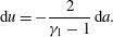
Reference McIntyre, Lourel, Eichmann, Morgan, Jacobs and Bishop2001), using the case-consistent set of gas properties from Step (b). Equation (6.1) relates the differential change in gas velocity through the unsteady expansion,
$\text{d}u$
, to the change in speed of sound,
$\text{d}a$
, as follows: (6.1)
$$\begin{eqnarray}\text{d}u=-\frac{2}{{\it\gamma}_{1}-1}\,\text{d}a.\end{eqnarray}$$
-
(d) As in § 4, a look-up-table was populated with region 2 flow properties for a matrix comprised of test gas shock speeds varying between
$u_{s,1}=400$
and
$11\,000~\text{m}~\text{s}^{-1}$
, with test gas fill pressures varying between
$p_{1}=10^{2}$
and
$10^{6}~\text{Pa}$
. Noting that the test gas always undergoes an unsteady expansion into the acceleration tube,
$u_{s,1}$
was calculated for each
$\{u_{s,5},p_{5},p_{1}\}$
combination. This entailed an iterative solution process which identified the unique combinations of
$p_{1}$
and
$u_{s,1}$
for which: (i)
$p_{2},u_{2}$
values intersected the
$p,u$
curves derived in Step (c); and (ii) had the same entropy as Step (b).




An accurate and consistent equilibrium analysis requires calculation of the entire solution set
 $\{p_{1},u_{s,1},p_{5},u_{s,5}\}$
in order to determine the two variables of interest for this study,
 $\{p_{1},u_{s,1}\}$
. Once these are known, they can be compared against the X2 driver performance envelope previously shown in figure 9. Figure 11 shows each of the flow conditions from tables 4–6, mapped onto figure 9. Three key observations can be made:
-
(a) When a secondary driver is used, each target test condition can be achieved across a range of static pressures; there is a theoretical capacity to control the test flow static pressure even though the primary driver configuration is fixed.
-
(b) The majority of the low-enthalpy scramjet conditions are only achieved in a region of the facility operating envelope where the secondary driver reduces net performance, even though the secondary driver itself is over-tailored.
-
(c) As the flight enthalpy increases, the range of
$p_{1}$
is reduced; for example, it can be seen that the
$16~\text{km}~\text{s}^{-1}$
Far Solar System return condition can be achieved only across a very narrow range of
$p_{1}$
. The reason for this is that the acceleration tube fill pressure was constrained to be
$p_{5}\geqslant 0.1~\text{Pa}$
; this constraint was applied since viscous effects become overwhelming at fill pressures lower than this.


The results of figure 11 are now considered separately by examining in detail two of each of the high- and low-enthalpy conditions.
7. Results and analysis
7.1. High-enthalpy examples:
$13$
and
$11~\text{km}~\text{s}^{-1}$
Mars return


Table 7 shows the calculated facility operating parameters for the
 $13~\text{km}~\text{s}^{-1}$
Mars return case (Case 1 in figure 11). The test flow static pressure,
 $p_{7}$
, is observed to vary with
 $p_{sd1}$
, and achieves a peak of
 $p_{7}=1.82~\text{kPa}$
for
 $p_{sd1}=112~\text{kPa}$
. Table 7 also shows
 $p_{7}$
for operation without a secondary driver;
 $p_{7}=1.17~\text{kPa}$
for Case 1d. For this flow condition case, the secondary driver can theoretically provide an increase in test flow static pressure of up to 56 %.
Calculated facility operating parameters for Mars return
 $13~\text{km}~\text{s}^{-1}$
Mach 10 equivalent flight.

For comparison, the Mach 10 true flight equivalent static pressure is 2.38 kPa (from figure 10), and is therefore marginally higher than what X2 can achieve with this specific free-piston driver condition. Nevertheless, these results confirm that the secondary driver can significantly outperform the basic expansion tube.
Figure 12(a) shows experimental confirmation of these results in X2. Measuring the speed of the primary shock as it traverses the length of the facility is an effective means to validate several of the key flow processes occurring during an experiment. It can be seen that there is generally good agreement with computed shock speeds through both the secondary driver and shock tube, although all except Case 1a have the experimental
 $u_{s,1}$
slightly less than the computed value.
Experimental results for
 $13~\text{km}~\text{s}^{-1}$
Mars return flight equivalent conditions; (a) shock speeds along the entire driven tube; (b) shock tube static pressures; static pressure traces are time-referenced to Case 1a, with offsets of
 $50~{\rm\mu}\text{s}$
,
 $100~{\rm\mu}\text{s}$
and
 $150~{\rm\mu}\text{s}$
, for Cases 1b, 1c and 1d, respectively.

It is noted that there is some scatter and uncertainty in the acceleration tube shock speeds; this was due to two reasons: firstly, the pressure sensors in this tube were insufficiently sensitive to precisely identify shock arrival at the transducer for these very low pressure conditions; secondly, low fill pressures could not be reliably achieved, or held, at the time of the experiments. Neither of these issues was of concern, since the important measurements were in the secondary driver and shock tube. However, these issues could be readily addressed in any future study requiring use of the final expanded test flow. Uncertainties in the secondary driver and shock tube are much lower, and in most cases the error bars, which are included in the plot, are too small to identify.
Figure 12(b) shows a tube wall static pressure measurement towards the end of the shock tube,
 $p_{2}$
, for Cases 1a–1d. Comparing these traces to the computed value of
 $p_{2}$
in table 7, it can be seen that all four experimental traces are 10–20 % lower in magnitude. This discrepancy probably reflects the slightly lower experimental shock speeds which were measured in the shock tube. However, the important observation is that a significantly larger static pressure is observed for Case 1b compared to the other conditions, as predicted by table 7, confirming that the secondary driver can be used as a test gas static pressure control.
The same analysis was repeated for the
 $11~\text{km}~\text{s}^{-1}$
Mars return condition (Case 4 in figure 11), with results shown in table 8 and figure 13. This example illustrates how the secondary driver can be used to reduce performance. Referring to table 8, Case 1a theoretically has
 $p_{7}=2.1~\text{kPa}$
, compared to
 $p_{7}=5{-}6~\text{kPa}$
for Cases 1b–1e. This is reflected by a much lower static pressure in the shock tube (figure 13
b); the relative difference is not as large as predicted by table 8, and is primarily due to the Case 4b experimental shock speeds being higher than the other conditions.
Calculated facility operation parameters for Mars return
 $11~\text{km}~\text{s}^{-1}$
Mach 10 equivalent flight.

Experimental results for
 $11~\text{km}~\text{s}^{-1}$
Mars return flight equivalent conditions; (a) shock speeds along the entire driven tube; (b) shock tube static pressures; static pressure traces are time-referenced to Case 4a, with offsets of
 $50~{\rm\mu}\text{s}$
,
 $100~{\rm\mu}\text{s}$
,
 $150~{\rm\mu}\text{s}$
and
 $200~{\rm\mu}\text{s}$
for Cases 4b, 4c, 4d and 4e, respectively.

In summary, the 11 and
 $13~\text{km}~\text{s}^{-1}$
Mars return results validate the driver characterisation detailed in Gildfind et al. (Reference Gildfind, James and Morgan2015), and show that the analytical techniques presented in this paper correctly predict the trends for facility performance, both with and without a secondary driver, and show that test gas static pressure can be controlled using the secondary driver.
7.2. Low-enthalpy examples: Mach
$10$
and Mach
$14$
scramjet flight


Tables 9 and 10 show calculated facility parameters for the Mach 10 (Case 2) and Mach 14 (Case 3) scramjet flow conditions from figure 11. However, recent experience with these conditions (Gildfind Reference Gildfind2012; Gildfind et al.
Reference Gildfind, Morgan, McGilvray and Jacobs2014) has shown that these calculations become invalid for facility configurations when there is a strong reflected shock through the secondary driver gas. Referring to figure 14 (originally from Gildfind et al.
Reference Gildfind, Morgan, McGilvray and Jacobs2014), when the secondary diaphragm ruptures, the shock-processed slug of helium (region
 $sd2$
) has a short length but high sound speed, and is rapidly processed by the reflected shock wave (c in the figure). This wave then reflects off the
 $sd2/sd3$
interface, and returns as a strong compression wave (d and e in figure 14). The time scales for this phenomenon are very short compared to other flow processes; for most practical conditions, the secondary driver would need to be an order of magnitude longer than the shock tube to sufficiently delay arrival of this wave. These wave processes have been described in Gildfind et al. (Reference Gildfind, Morgan, McGilvray and Jacobs2014); however, the broader implications of those results were not examined at the time.
L1d-computed
 $x{-}t$
diagram for Mach 10 scramjet flow condition in X2. Contours show log of static pressure (in units log (Pa)). (Points on
 $x{-}t$
diagram: (a) Primary diaphragm is downstream of driver area change; compression wave is transmitted downstream from this area change. (b) Arrival of compression wave at primary shock increases shock speed. (c) Reflected shock arises at secondary diaphragm due to primary shock arrival at dense test gas. (d) Reflected shock hits contact surface and a second compression wave is sent downstream. (e) Second compression wave arrives at primary shock and causes a second primary shock speed increase.) Adapted from Gildfind et al. (Reference Gildfind, Morgan, McGilvray and Jacobs2014, figure 9).

In practice, at low-enthalpy conditions with a dense test gas, the secondary driver behaviour is no longer adequately described by traditional theoretical models. The helium has negligible effect on the magnitude of test flow properties, and acts as a passive slug between the primary driver and test gases. This effect is shown in figure 15(a,b) for the Case 2 scramjet Mach 10 condition. In both plots, the 1-D computational fluid dynamics (CFD) code L1d (Jacobs Reference Jacobs1994) has been used to calculate shock speeds along the length of X2, where
 $x=0$
corresponds to the primary diaphragm location. These L1d models use a constant volume driver (with initial temperature and pressure as defined in table 1), instead of a free-piston driver, in order to provide a more direct comparison to the analytical calculations summarised in figure 11. The driver length in the L1d model was made sufficiently long to avoid interference of the reflected driver
 $u+a$
wave during the useful test time.
Shock speeds for X2 Mach 10 scramjet flow conditions detailed in table 9; (a) shows shock speeds for Cases 2a–2f; solid lines are L1d CFD calculations; dashed lines are calculated using the equilibrium analysis in § 6; datapoints are experimental results; (b) shows L1d shock speeds for Case 2f operated with and without a secondary driver, for a wide range of secondary driver fill pressures.

Calculated facility configurations for Mach 10 scramjet flight.

Calculated facility configurations for Mach 14 scramjet flight.

Referring to figure 15(a), the Case 2a–2e curves show shock speeds when secondary drivers of differing fill pressures are introduced between the primary diaphragm (
 $x=0$
) and
 $x=3.4~\text{m}$
; the case 2f curve shows the shock speed for a Mach 10 scramjet condition without a secondary driver. Dashed lines show the corresponding ‘target’ shock speeds at each condition; these are the shock speeds predicted by analytical techniques (see table 9), which should theoretically achieve the flow conditions shown in figure 11. It is clear in figure 15(a) that the L1d-computed shock speeds match the target speeds reasonably well through the secondary driver; however, L1d predicts higher shock speeds through the downstream shock and acceleration tubes.
L1d, which has been shown to reliably predict shock speeds in recent scramjet flow condition studies using UQ’s X2 and X3 facilities (Gildfind Reference Gildfind2012; Gildfind et al.
Reference Gildfind, Sancho and Morgan2013, Reference Gildfind, Morgan, McGilvray and Jacobs2014), takes into account the full set of longitudinal wave processes. As with the Gildfind et al. (Reference Gildfind, Morgan, McGilvray and Jacobs2014) study, the reinforcing compression wave from the driver, which is captured by L1d, causes an increase in the shock speed above the target level. Referring to the red ‘
 $Ma10$
’ curve in figure 11, it can be seen that as the secondary driver fill pressure is reduced, the secondary driver is predicted by analytical techniques to become increasingly ineffective at driving a shock into the air test gas. This explains why the downstream fill pressures in table 9,
 $p_{1}$
and
 $p_{5}$
, become correspondingly lower in order to achieve the same shock speeds. However, since the reinforcing compression wave (d and e in figure 14) essentially restores the full strength of the driver, then higher shock speeds are predicted at these lower fill pressures in figure 15.
Figure 15(b) demonstrates the ineffectiveness of the secondary driver at lower enthalpies from a different perspective. This figure shows L1d-computed shock speeds for flow condition ‘Case 2f’, which is designed for X2 without a secondary driver. The black curve in figure 15(b) is shown to match the ‘target’ shock speeds very closely (note, for this L1d simulation the shock tube runs from
 $x=0$
to
 $x=3.4~\text{m}$
). The other curves show shock speeds for the same condition, except in each case a helium secondary driver is introduced between
 $x=0$
and
 $x=3.4~\text{m}$
. Each of these curves represents a different secondary driver fill pressure, across a range spanning 1–1000 kPa. While computed shock speeds evidently vary through the secondary driver, all curves are seen to collapse to the same speeds further downstream in the shock tube. This result shows that the final magnitude of the test flow properties is unaffected by the inclusion of a helium secondary driver once driver secondary wave processes are accounted for. Thus the theoretical predictions of figure 11 are shown to be invalid. At low enthalpies, where a reflected shock processes the secondary driver gas, the theoretical test gas shock speed is not achieved due to the driver wave coupling.
Referring to figure 15(a), it is noted that shock speeds for Cases 2b–2d have been validated by experiment with X2, and good agreement is observed. Error bars are plotted but are not obvious since experimental uncertainties for these shock speeds are low. The remaining shock speeds in figure 15(a,b) were not experimentally validated due to the impractical shock tube fill pressures required for these conditions (100 Pa for Case 2a; 1551 kPa for all of the Case 2f conditions). The 1551 kPa fill pressure exceeds the current manifold and instrumentation pressure rating for X2, and is only required to be this high in the example to match the high performance of this particular free-piston driver condition.
Shock speeds for X2 Mach 14 scramjet flow conditions detailed in table 10; (a) shows shock speeds for Cases 3a–3e; solid lines are L1d CFD calculations; dashed lines are calculated using the equilibrium analysis in § 6; datapoints are experimental results; (b) shows L1d shock speeds for Case 3e operated with and without a secondary driver, for a wide range of secondary driver fill pressures; datapoints are experimental results.

More comprehensive validation was undertaken for the Mach 14 flow condition. Figures 16(a,b) are Mach 14 equivalents of the figure 15(a,b) Mach 10 plots. Full validation at Mach 14 was possible since the maximum shock tube fill pressure was lower (548 kPa). Identical trends are observed in figure 16, thereby supporting earlier conclusions about the secondary driver operation at low-enthalpy conditions. The computed shock speeds match experiment closely through the secondary driver and shock tube. Case 3e (no secondary driver) also indicates good agreement between L1d and experiment; however, all of the secondary driver conditions have slower experimental shock speeds through the acceleration tube than those predicted by L1d. The cause of this discrepancy was not established, since the secondary driver and shock tube measurements were the most relevant results for this secondary driver study, and examination of acceleration tube flow processes would have required computationally intensive axisymmetric CFD of the facility, across several conditions. However, a consistent difference with the secondary driver conditions was the relatively short acceleration tube, arising due to the addition of a third diaphragm. With a shorter acceleration tube the test flow is more influenced by shock establishment and interface mixing, and the test gas is not fully utilised. This issue would need to be re-examined before X2 was used for these specific operating conditions, and normally extension tubes would be added to lengthen the acceleration tube for such experiments.
7.3. Secondary driver as acoustic buffer, and test time implications
As discussed in § 2.3, Morgan & Stalker (Reference Morgan and Stalker1991) proposed the use of a secondary driver to act as an ‘acoustic buffer’ for these types of scramjet conditions, because it had earlier been shown that over-tailored operation could prevent the transmission of driver disturbances from the expanded primary driver gas to the test gas (Paull & Stalker Reference Paull and Stalker1992). Figure 17 demonstrates this ‘acoustic buffer’ using L1d simulations of X2, incorporating full piston dynamics, for the ‘case 2f’ Mach 10 condition in figure 15 and table 9. Figure 17(a) shows sound speed mapped over an
 $x{-}t$
diagram for the basic expansion tube; figure 17(a) shows the same result with a helium secondary driver initially at 150 kPa. It can be seen that, without a secondary driver, the ratio
 $a_{2}/a_{3}\ll 1$
, and driver noise would be expected to transmit to the test gas (Paull & Stalker Reference Paull and Stalker1992); figure 17(b), however, shows that the inclusion of a secondary driver strongly over-tailors the interface to the primary driver gas (i.e.
 $a_{sd2}/a_{sd3}\gg 1$
), thereby meeting the acoustic buffer requirement.
Computed sound speed for Mach 10 scramjet condition (a) without and (b) with 150 kPa helium secondary driver.

While this arrangement would theoretically shield the downstream gas from primary driver disturbances, the air (region 2) is still under-tailored with respect to region 3; disturbances arising in the secondary driver gas due to Mylar diaphragm rupture, or the flow’s passage down the tube, could theoretically be transmitted to the test gas this way. Since the test gas itself lacks the intrinsic mechanism to prevent noise ingress, it might be expected that these conditions should be somewhat noisier than conditions where the test gas itself provides the acoustic buffer. Furthermore, for scramjet flow conditions, the secondary driver gas will be processed by a reflected shock, and the effect, if any, of this shock on transmission of acoustic disturbances has not been studied in detail.
Recalling figure 16(b), the Mach 14 scramjet flow condition, Case 3e, was experimentally tested with and without a secondary driver, and at a range of different secondary driver fill pressures. For these experiments a flow impact pressure measurement was made at the tube exit using 15° half-angle cone probes. These probes are described in Gildfind et al. (Reference Gildfind, Morgan, McGilvray and Jacobs2014), and were developed for earlier scramjet flow condition testing. The probe has a conical face in order to reduce heating, pressure loading and impact damage to the transducer sensing face, and to provide a generally less severe measurement than a blunt-body Pitot probe. Two probes were placed at radial offsets of
 $\pm 9~\text{mm}$
around the tube centreline, in accordance with the configuration shown in figure 18(a); cone pressure measurements are shown in figure 18(b–f) for the cases shown in figure 16(b).
Cone pressures for X2 Mach 14 scramjet flow condition, Case 3e from table 10, operated with and without a secondary driver, for a wide range of secondary driver fill pressures: (a) cone probe configuration; (b) no secondary driver (shot x2s2784); (c) 1 kPa secondary driver (shot x2s2787); (d) 10 kPa secondary driver (shot x2s2788); (e) 100 kPa secondary driver (shot x2s2789); (f) 398 kPa secondary driver (shot x2s2757).

Figure 18(b) shows the cone pressure traces for Case 3e without a secondary driver. A
 $100~{\rm\mu}\text{s}$
period of approximately steady cone pressure (
 ${\approx}100~\text{kPa}$
) is identified on the two traces. Through this region high-frequency noise can be observed, causing a fluctuation of approximately
 $\pm 10\,\%$
about the mean. After this period of identified test time, the cone impact pressure rises due to the test gas being underexpanded, higher temperature, lower Mach number, and therefore departing too far from the target flow condition.
The same condition is then shown with a range of secondary driver fill pressures in figure 16(c–f). Unsurprisingly, all of these cone pressure traces have a similar magnitude, which is lower than figure 16(b), and which is consistent with the lower experimental shock speeds shown in figure 16(b). Two differences are apparent; firstly, each cone pressure is increasing during the passage of the test gas, which arrives after the accelerator gas (the accelerator gas is the initial region of low impact pressure). For the purposes of comparison, the region of test time is identified as the region where cone pressures are 50–100 kPa; however, a test gas with this pressure gradient would not be useful for practical experiments. The test time according to this definition is approximately half the duration of the case without a secondary driver.
The second observation is that figures 16(c–e) do not exhibit the high-frequency noise of figure 16(b). This supports the argument that the secondary driver has suppressed disturbance transmission to the test gas. Observing 16(f), this is actually Case 3d; observing figure 11, the driver sound speed ratio is matched at this condition (
 $a_{sd2}=a_{3}$
), therefore this condition would be expected to be noisier, and this is observed.
The results from figure 16 suggest that further analysis is required to validate the acoustic buffer function of the secondary driver. While the secondary driver appears to reduce high-frequency noise in the cone pressure traces, it can be seen in figure 16 that useful test time is significantly reduced, and the impact pressure measurements do not exhibit a suitable period of test gas with steady flow properties. Studying and optimising the acoustics and wave processes of this mode of operation is beyond the scope of the current paper, and is part of an ongoing separate investigation.
The short test times of
 $50{-}100~{\rm\mu}\text{s}$
are not sufficient for scramjet engine tests, which usually require much longer duration test flows than high-enthalpy planetary entry studies. Anderson, Kumar & Erdos (Reference Anderson, Kumar and Erdos1990) suggests minimum test time requirements to achieve flow establishment inside a scramjet engine as follows:
 $$\begin{eqnarray}\displaystyle & tu/L\geqslant 2\quad \text{for attached turbulent flow}, & \displaystyle\end{eqnarray}$$
 $$\begin{eqnarray}\displaystyle & tu/L\geqslant 3\quad \text{for attached laminar flow}, & \displaystyle\end{eqnarray}$$
 $t$
is the test time,
 $u$
is the flow velocity and
 $L$
is the overall model length. For a reasonably large 1 m long model at Mach 10 (
 $3011~\text{km}~\text{s}^{-1}$
from table 6), the test time would therefore need to exceed
 $3\times 1.0/3011=1~\text{ms}$
, which is at least an order of magnitude higher than the test times identified in figure 18. However, this does not preclude expansion tubes from scramjet testing.
Details of X3 Mach 10 scramjet test flow experiment: (a) X3 expansion tube facility schematic; (b) X3 Pitot rake arrangement; (c) probe detail; (d) Pinckney probe pressure measurement; (e) cone probe pressure measurements.

The high total pressure capability of expansion tubes allows testing of smaller models through binary (
 ${\it\rho}{-}L$
) scaling, and test time can also be increased through the use of a contoured nozzle (Stewart, Jacobs & Morgan Reference Stewart, Jacobs and Morgan2001). McGilvray et al. (Reference McGilvray, Morgan and Jacobs2010) used X2 in the basic expansion tube mode (no secondary driver) with a contoured nozzle, to test a 2∕5 scale, 0.5 m long 2-D scramjet. These results compared well with tests of the full-scale engine in UQ’s T4 RST facility, at equivalent
 ${\it\rho}{-}L$
product.
For testing of larger engines, the problem of test time is directly addressed by using a large facility. Scramjet engine testing in X2 (McGilvray et al. Reference McGilvray, Morgan and Jacobs2010) and X2 flow condition development (Gildfind et al. Reference Gildfind, Morgan, McGilvray and Jacobs2014) were both conducted primarily as proof-of-concept studies in preparation for scaling up to UQ’s much larger free-piston-driven X3 facility. At 65 m length, with a 183 mm acceleration tube bore, X3 has equivalent total pressure capability to X2, but can test much larger models, and for significantly longer test times.
Figure 19(a) shows a scaled drawing of X3, which has recently been used to generate Mach 10 scramjet test flows in support of scramjet engine testing (Gildfind et al. Reference Gildfind, Sancho and Morgan2013). As part of the flow condition development process, nozzle exit flow measurements were made with the Pitot rake shown in figure 19(b). This rake was instrumented primarily with the cone probes also shown in figure 18, as well as a quasi-static-pressure ‘Pinckney’ probe (Pinckney Reference Pinckney1975). Referring to figure 19(d,e), the useful test time is approximately 1.25 ms, with a core flow diameter of 200 mm (using X3’s Mach 10 440 mm inner exit diameter nozzle). Noting that this condition used a secondary driver, cone impact pressures are much steadier than those shown in figure 18, although there remains a pressure gradient during the test time.
Figure 19 illustrates the potential for large expansion tubes to achieve an equivalent test time and model size capability to that of large RST facilities, but at much higher total pressures.
8. Key observations
Several observations have been made with respect to expansion tube operation with a secondary driver, which are summarised as follows:
-
(a) As previous analyses have shown (Henshall Reference Henshall1956; Stalker & Plumb Reference Stalker and Plumb1968; Morgan & Stalker Reference Morgan and Stalker1991; Morgan Reference Morgan, Ben-Dor, Igra and Elperin2001a ), an over-tailored secondary driver can drive a stronger shock than the primary driver by itself. The region of performance increase is bounded by two requirements: firstly, the secondary driver must be over-tailored, i.e. (
$a_{sd2}>a_{3}$
); secondly, the secondary driver gas must undergo an unsteady expansion upon impacting the test gas. -
(b) Within the region of performance gain, the secondary driver can be used as a static pressure control. In a basic expansion tube, there is only one combination of test flow static pressure, temperature and velocity, which can be achieved with a fixed primary driver configuration. This study has shown that introducing a secondary driver allows test flow static pressure to be varied widely for otherwise identical flow conditions (in terms of velocity, temperature and, therefore, Mach number). Analytical calculations corrected for chemical equilibrium effects have been shown to be sufficient to utilise this capability.
-
(c) In over-tailored operation, the generation of a reflected shock instead of an unsteady expansion between the region
$sd2$
/3 interface will result in reduced performance compared to operation without a secondary driver. -
(d) Figure 7 shows the density ratio
${\it\rho}_{sd1}/{\it\rho}_{1}$
below which a reflected shock will arise, based on an ideal gas analysis; in the limiting case,
${\it\rho}_{sd1}/{\it\rho}_{1}<1$
will produce a reflected shock and therefore a performance drop. For (relatively) heavy test gases such as air, this proves to be a restrictive condition which effectively limits the secondary driver as a performance-increasing device to superorbital conditions only, since the test gas (air) must initially be at a lower density than the secondary driver (helium). However, this is less restrictive when lighter test gases are used (for example, Gas Giant flows comprised primarily of helium and hydrogen, which can have order-of-magnitude lower molecular masses). -
(e) Morgan & Stalker (Reference Morgan and Stalker1991) identified an additional use for the secondary driver: in over-tailored operation it can theoretically provide the necessary acoustic buffer (Paull & Stalker Reference Paull and Stalker1992) to prevent ingress of driver-induced flow disturbances to the test gas, where such a buffer would not exist with the primary driver alone. Figure 17 shows the practical implementation of this principle for a theoretical scramjet Mach 10 condition. Operation with and without a secondary driver was experimentally examined for a Mach 14 flow condition; it was found that (i) acceleration tube shock speeds were consistently lower when using a secondary driver, even though shock tube shock speeds were more closely matched; (ii) cone impact pressure measurements indicated a period of approximately constant pressure without a secondary driver, but were constantly rising during the test time (with no apparent steady region) with a secondary driver; results from the larger X3 facility indicate a less severe pressure gradient, therefore it does not necessarily appear to be intrinsic to the secondary driver; (iii) high-frequency noise appeared to be significantly reduced when the secondary driver was used, so long as it was over-tailored.
-
(f) Considering the secondary driver as an acoustic buffer, this study has demonstrated that most practical flow conditions which would benefit from this arrangement will have a strong reflected shock through the secondary driver gas. It has been shown in this paper that this reflected shock reflects from the
$sd3$
/
$sd2$
region interface, resulting in a subsequent upstream running compression wave. For most practical arrangements, this compression wave will arrive at the test gas long before the test gas reaches the test section, and its effect on test gas acoustics needs to be assessed. -
(g) This upstream running compression wave invalidates 0-D theoretical estimates of the flow in this operating mode, since the wave processes become strongly coupled. In simple terms, the helium secondary driver gas becomes a passive intermediate gas slug which is compressed between the expanded driver gas and shock-processed test gas. It ceases to significantly influence the bulk test flow properties, which instead approach the equivalent properties for operation without a secondary driver, albeit those for a shorter tube.
-
(h) The ideal gas theoretical analysis of § 3 demonstrated the same qualitative trends as the specific performance analysis of X2 using equilibrium chemistry in §§ 4–7. This provides confidence that the observations from the X2 study will be applicable to expansion tubes generally.


Future efforts need to address the following remaining questions:
-
(a) For the low-enthalpy case, where the secondary driver is processed by a reflected shock, whether or not the secondary driver remains effective as an acoustic buffer in accordance with the original analysis by Paull & Stalker (Reference Paull and Stalker1992).
-
(b) For configurations where the secondary driver is over-tailored in relation to the primary driver gas, the test gas (region 2) may still be under-tailored in relation to the shock-processed secondary driver gas (region
$sd2$
); in such cases, it is necessary to establish what amount of noise is present in the secondary driver gas due to secondary diaphragm rupture and passage down the tube, and whether or not this noise transmits to the test gas and degrades the test flow quality. -
(c) Determine if there is an ideal ratio of over-tailoring of the secondary driver gas, and under-tailoring of the test gas, that leads to an optimal test flow.

9. Conclusion
This paper has provided an overview of results from a study of expansion tube operation with a secondary driver. Facility performance across the entire practical operating envelope of the X2 facility has been assessed. It has been shown that operating characteristics can vary significantly, and depend primarily on the initial density ratio between the secondary driver gas and test gas. When the secondary driver gas is denser than the test gas, it undergoes an unsteady expansion into the test gas, and a theoretical performance increase can be achieved. When the test gas is denser, the secondary driver gas is instead processed by a reflected shock, which becomes coupled to primary driver wave processes. This complicates local flow processes, and subsequently invalidates traditional analytical performance estimates.
Acknowledgements
The authors wish to thank the Australian Research Council and the Queensland Smart State Research Facilities Fund 2005 for support and funding. The authors also wish to thank F. De Beurs for technical assistance with X2.
Appendix A. Analytical solution procedure for prediction of expansion tube flow processes
A.1. Basic free-piston driver with area change
This appendix considers a free-piston-driven shock tube with driver area change. Referring to figure 1, and assuming that the following quantities are initially specified:
-
(i)
$T_{4,i}$
and
$T_{1}$
; initial temperatures of driver gas and test gas; -
(ii)
${\it\lambda}$
; compression ratio of driver gas after free-piston compression; -
(iii)
$p_{4}/p_{1}$
; ratio between driver gas and test gas pressures at moment of diaphragm rupture; -
(iv)
${\it\gamma}_{4}$
and
${\it\gamma}_{1}$
; driver and test gas specific heat ratios; -
(v)
$R_{4}$
and
$R_{1}$
; driver and test gas specific gas constants.


The driver gas is compressively heated from its initial fill temperature,
 $T_{4,i}$
, to its temperature at rupture,
 $T_{4}$
:
 $$\begin{eqnarray}T_{4}=T_{4,i}{\it\lambda}^{{\it\gamma}_{4}-1}.\end{eqnarray}$$
When the diaphragm ruptures, the initially stagnant driver gas (
 $T_{4}=T_{4,0}$
) begins to expand into the driven tube. An unsteady expansion processes the driver gas from region 4 to region
 $4^{\prime }$
. For large area reductions from the driver to driven tubes, it is reasonable to assume that there are negligible total pressure and temperature losses through this subsonic driver gas expansion (Morgan Reference Morgan, Ben-Dor, Igra and Elperin2001b
):
 $$\begin{eqnarray}T_{4}=T_{4,0}\approx T_{4^{\prime }}\approx T_{4^{\prime },0}.\end{eqnarray}$$
A steady expansion then processes the driver gas to state
 $4^{\prime \prime }$
across the area change. The Mach number is 1.0 since the flow is choked:
 $$\begin{eqnarray}Ma_{4^{\prime \prime }}=1.0.\end{eqnarray}$$
Stagnation and static properties are related as follows through the steady expansion:
 $$\begin{eqnarray}{\displaystyle \frac{T_{4^{\prime \prime },0}}{T_{4^{\prime \prime }}}}=1+{\displaystyle \frac{{\it\gamma}_{4}-1}{2}}Ma_{4^{\prime \prime }}^{2}.\end{eqnarray}$$
The total temperature and pressure remain constant through the steady expansion; substituting
 $T_{4^{\prime \prime },0}=T_{4^{\prime },0}$
, equations (A 2) and (A 3) into (A 4):
 $$\begin{eqnarray}T_{4^{\prime \prime }}={\displaystyle \frac{2T_{4}}{{\it\gamma}_{4}+1}}.\end{eqnarray}$$
The velocity across the area change is as follows:
 $$\begin{eqnarray}u_{4^{\prime \prime }}=a_{4^{\prime \prime }}=\sqrt{{\it\gamma}_{4}R_{4}T_{4^{\prime \prime }}}.\end{eqnarray}$$
Assuming isentropic flow from regions 4 to
 $4^{\prime \prime }$
:
 $$\begin{eqnarray}{\displaystyle \frac{p_{4^{\prime \prime }}}{p_{4}}}=\left({\displaystyle \frac{T_{4^{\prime \prime }}}{T_{4}}}\right)^{{\it\gamma}_{4}/({\it\gamma}_{4}-1)}.\end{eqnarray}$$
Across the unsteady expansion between regions
 $4^{\prime \prime }$
and 3, velocity and sound speed are related as follows:
 $$\begin{eqnarray}u_{3}+{\displaystyle \frac{2a_{3}}{{\it\gamma}_{3}-1}}=u_{4^{\prime \prime }}+{\displaystyle \frac{2a_{4^{\prime \prime }}}{{\it\gamma}_{4}-1}}.\end{eqnarray}$$
Noting (A 6), that
 ${\it\gamma}_{3}={\it\gamma}_{4}$
, substituting these into (A 8) and rearranging:
 $$\begin{eqnarray}u_{3}={\displaystyle \frac{a_{4^{\prime \prime }}({\it\gamma}_{4}+1)-2a_{3}}{{\it\gamma}_{4}-1}}={\displaystyle \frac{\sqrt{{\it\gamma}_{4}R_{4}}}{{\it\gamma}_{4}-1}}[\sqrt{T_{4^{\prime \prime }}}({\it\gamma}_{4}+1)-2\sqrt{T_{3}}].\end{eqnarray}$$
The induced flow velocity behind the shock in region 2,
 $u_{2}$
, is given by standard shock relations:
 $$\begin{eqnarray}u_{2}={\displaystyle \frac{a_{1}}{{\it\gamma}_{1}}}\left({\displaystyle \frac{p_{2}}{p_{1}}}-1\right)\left[{\displaystyle \frac{\displaystyle {\displaystyle \frac{2{\it\gamma}_{1}}{{\it\gamma}_{1}+1}}}{\displaystyle {\displaystyle \frac{p_{2}}{p_{1}}}+{\displaystyle \frac{{\it\gamma}_{1}-1}{{\it\gamma}_{1}+1}}}}\right]^{1/2}.\end{eqnarray}$$
The pressure in region 3 is equal to region 2, i.e.
 $p_{3}=p_{2}$
, therefore temperature in region 3 can be calculated from isentropic relations:
 $$\begin{eqnarray}\displaystyle & \displaystyle {\displaystyle \frac{p_{3}}{p_{4^{\prime \prime }}}}={\displaystyle \frac{p_{2}}{p_{4^{\prime \prime }}}}={\displaystyle \frac{p_{2}}{p_{4}}}\cdot {\displaystyle \frac{p_{4}}{p_{4^{\prime \prime }}}}={\displaystyle \frac{p_{2}}{p_{1}}}\cdot {\displaystyle \frac{p_{1}}{p_{4}}}\cdot {\displaystyle \frac{p_{4}}{p_{4^{\prime \prime }}}}, & \displaystyle\end{eqnarray}$$
 $$\begin{eqnarray}\displaystyle & \displaystyle T_{3}=T_{4^{\prime \prime }}\left({\displaystyle \frac{p_{3}}{p_{4^{\prime \prime }}}}\right)^{({\it\gamma}_{4}-1)/{\it\gamma}_{4}}=T_{4^{\prime \prime }}\left({\displaystyle \frac{p_{2}}{p_{1}}}\cdot {\displaystyle \frac{p_{1}}{p_{4}}}\cdot {\displaystyle \frac{p_{4}}{p_{4^{\prime \prime }}}}\right)^{({\it\gamma}_{4}-1)/{\it\gamma}_{4}}. & \displaystyle\end{eqnarray}$$
Substituting (A 12) into (A 9) and noting that
 $u_{2}=u_{3}$
across the interface:
 $$\begin{eqnarray}{\displaystyle \frac{a_{1}}{{\it\gamma}_{1}}}\left({\displaystyle \frac{p_{2}}{p_{1}}}-1\right)\left[{\displaystyle \frac{\displaystyle {\displaystyle \frac{2{\it\gamma}_{1}}{{\it\gamma}_{1}+1}}}{\displaystyle {\displaystyle \frac{p_{2}}{p_{1}}}+{\displaystyle \frac{{\it\gamma}_{1}-1}{{\it\gamma}_{1}+1}}}}\right]^{1/2}={\displaystyle \frac{\sqrt{{\it\gamma}_{4}R_{4}T_{4^{\prime \prime }}}}{{\it\gamma}_{4}-1}}\left[{\it\gamma}_{4}+1-2\left({\displaystyle \frac{p_{2}}{p_{1}}}\cdot {\displaystyle \frac{p_{1}}{p_{4}}}\cdot {\displaystyle \frac{p_{4}}{p_{4^{\prime \prime }}}}\right)^{({\it\gamma}_{4}-1)/2{\it\gamma}_{4}}\right].\end{eqnarray}$$
After evaluating (A 1), (A 5) and (A 7), (A 13) can be used to solve for the resulting shock pressure ratio
 $p_{2}/p_{1}$
.
A.2. Compound driver with area change
A free-piston-driven shock tube, with a secondary driver between the primary diaphragm and shock tube, is now considered. Referring to either figure 3 or 5, the configuration parameters are the same as in § A.1, except the following initial quantities must additionally be specified:
-
(i)
$T_{sd1}$
; initial temperature in secondary driver; -
(ii)
$p_{sd1}/p_{1}$
; initial ratio of secondary driver and test gas pressure ratios; -
(iii)
${\it\gamma}_{sd}$
; secondary driver ratio of specific heats; -
(iv)
$R_{sd}$
; secondary driver specific gas constant.


The shock speed through the secondary driver can be calculated by solving (A 15) for the ratio
 $p_{sd2}/p_{sd1}$
; this equation is simply an adaptation of (A 13), with the additional substitution shown in (A 14):
 $$\begin{eqnarray}\displaystyle & \displaystyle {\displaystyle \frac{p_{sd1}}{p_{4}}}={\displaystyle \frac{p_{sd1}}{p_{1}}}\cdot {\displaystyle \frac{p_{1}}{p_{4}}}, & \displaystyle\end{eqnarray}$$
 $$\begin{eqnarray}\displaystyle & & \displaystyle \displaystyle {\displaystyle \frac{a_{sd1}}{{\it\gamma}_{sd}}}\left({\displaystyle \frac{p_{sd2}}{p_{sd1}}}-1\right)\left[{\displaystyle \frac{\displaystyle {\displaystyle \frac{2{\it\gamma}_{sd}}{{\it\gamma}_{sd}+1}}}{\displaystyle {\displaystyle \frac{p_{sd2}}{p_{sd1}}}+{\displaystyle \frac{{\it\gamma}_{sd}-1}{{\it\gamma}_{sd}+1}}}}\right]^{1/2}\nonumber\\ \displaystyle & & \displaystyle \quad ={\displaystyle \frac{\sqrt{{\it\gamma}_{4}R_{4}T_{4^{\prime \prime }}}}{{\it\gamma}_{4}-1}}\left[{\it\gamma}_{4}+1-2\left({\displaystyle \frac{p_{sd2}}{p_{sd1}}}\cdot {\displaystyle \frac{p_{sd1}}{p_{1}}}\cdot {\displaystyle \frac{p_{1}}{p_{4}}}\cdot {\displaystyle \frac{p_{4}}{p_{4^{\prime \prime }}}}\right)^{({\it\gamma}_{4}-1)/2{\it\gamma}_{4}}\right].\end{eqnarray}$$
Referring to figure 20, either an unsteady expansion (figure 20
b) or a reflected shock (figure 20
c) may process the region
 $sd2$
gas. Initially, an unsteady expansion will be assumed to occur; if the solution predicts a pressure drop from regions
 $p_{sd2}$
to
 $p_{3}$
, then the assumption will be considered valid. Otherwise, if
 $p_{sd2}<p_{3}$
, the assumption will be considered invalid, and the calculation must be repeated assuming a reflected shock.
Reflected shock and unsteady expansion solutions following secondary diaphragm rupture: (a) prior to shock arrival at secondary diaphragm; (b) after diaphragm rupture;
 $u_{3}>u_{sd2}$
and
 $p_{3}<p_{sd2}$
; (c) after diaphragm rupture;
 $u_{3}<u_{sd2}$
and
 $p_{3}>p_{sd2}$
; (d) reflected shock from (c) in shock steady coordinate system: s
 $=$
shock; rs
 $=$
reflected shock; cs
 $=$
contact surface; usx
 $=$
unsteady expansion.

A.2.1. Unsteady expansion at secondary diaphragm
Referring to figure 20(b), an unsteady expansion transforms the secondary driver gas from state
 $sd2$
to state 3. Equation (A 16) relates the flow properties across the unsteady expansion:
 $$\begin{eqnarray}u_{3}+{\displaystyle \frac{2a_{3}}{{\it\gamma}_{3}-1}}=u_{sd2}+{\displaystyle \frac{2a_{sd2}}{{\it\gamma}_{sd}-1}}.\end{eqnarray}$$
 $u_{sd2}$
and
 $T_{sd2}$
are given by (A 17) and (A 18), respectively, and can be calculated once (A 15) has been solved:
 $$\begin{eqnarray}\displaystyle & \displaystyle u_{sd2}={\displaystyle \frac{a_{sd1}}{{\it\gamma}_{sd}}}\left({\displaystyle \frac{p_{sd2}}{p_{sd1}}}-1\right)\left[{\displaystyle \frac{\displaystyle {\displaystyle \frac{2{\it\gamma}_{sd}}{{\it\gamma}_{sd}+1}}}{\displaystyle {\displaystyle \frac{p_{sd2}}{p_{sd1}}}+{\displaystyle \frac{{\it\gamma}_{sd}-1}{{\it\gamma}_{sd}+1}}}}\right]^{1/2}, & \displaystyle\end{eqnarray}$$
 $$\begin{eqnarray}\displaystyle & \displaystyle T_{sd2}=T_{sd1}{\displaystyle \frac{p_{sd2}}{p_{sd1}}}\left({\displaystyle \frac{\displaystyle {\displaystyle \frac{{\it\gamma}_{sd}+1}{{\it\gamma}_{sd}-1}}+{\displaystyle \frac{p_{sd2}}{p_{sd1}}}}{\displaystyle 1+{\displaystyle \frac{{\it\gamma}_{sd}+1}{{\it\gamma}_{sd}-1}}\cdot {\displaystyle \frac{p_{sd2}}{p_{sd1}}}}}\right). & \displaystyle\end{eqnarray}$$
Expanding sound speed terms in (A 16), noting that
 ${\it\gamma}_{3}={\it\gamma}_{sd}$
, and solving for
 $u_{3}$
:
 $$\begin{eqnarray}u_{3}=u_{sd2}+{\displaystyle \frac{2\sqrt{{\it\gamma}_{sd}R_{sd}}}{{\it\gamma}_{sd}-1}}(\sqrt{T_{sd2}}-\sqrt{T_{3}}).\end{eqnarray}$$
 $T_{3}$
is related to
 $T_{sd2}$
by isentropic relations:
 $$\begin{eqnarray}T_{3}=T_{sd2}\left({\displaystyle \frac{p_{3}}{p_{sd2}}}\right)^{({\it\gamma}_{sd}-1)/{\it\gamma}_{sd}}.\end{eqnarray}$$
Expanding (A 20) and noting that
 $p_{2}=p_{3}$
:
 $$\begin{eqnarray}T_{3}=T_{sd2}\left({\displaystyle \frac{p_{2}}{p_{1}}}\cdot {\displaystyle \frac{p_{1}}{p_{sd1}}}\cdot {\displaystyle \frac{p_{sd1}}{p_{sd2}}}\right)^{({\it\gamma}_{sd}-1)/{\it\gamma}_{sd}}.\end{eqnarray}$$
Substituting (A 21) into (A 19) and noting that
 $u_{3}=u_{2}$
(which was already provided in (A 10)):
 $$\begin{eqnarray}\displaystyle & & \displaystyle \displaystyle {\displaystyle \frac{a_{1}}{{\it\gamma}_{1}}}\left({\displaystyle \frac{p_{2}}{p_{1}}}-1\right)\left[{\displaystyle \frac{{\displaystyle \frac{2{\it\gamma}_{1}}{{\it\gamma}_{1}+1}}}{{\displaystyle \frac{p_{2}}{p_{1}}}+{\displaystyle \frac{{\it\gamma}_{1}-1}{{\it\gamma}_{1}+1}}}}\right]^{1/2}\nonumber\\ \displaystyle & & \displaystyle \quad =u_{sd2}+{\displaystyle \frac{2\sqrt{{\it\gamma}_{sd}R_{sd}T_{sd2}}}{{\it\gamma}_{sd}-1}}\left[1-\left({\displaystyle \frac{p_{2}}{p_{1}}}\cdot {\displaystyle \frac{p_{1}}{p_{sd1}}}\cdot {\displaystyle \frac{p_{sd1}}{p_{sd2}}}\right)^{({\it\gamma}_{sd}-1)/2{\it\gamma}_{sd}}\right].\end{eqnarray}$$
Equation (A 22) can be used to solve for the pressure ratio
 $p_{2}/p_{1}$
. The solution will be valid for
 $p_{3}/p_{sd2}<1$
; this ratio can be evaluated using (A 23):
 $$\begin{eqnarray}{\displaystyle \frac{p_{3}}{p_{sd2}}}={\displaystyle \frac{p_{2}}{p_{sd2}}}={\displaystyle \frac{p_{2}}{p_{1}}}\cdot {\displaystyle \frac{p_{1}}{p_{sd1}}}\cdot {\displaystyle \frac{p_{sd1}}{p_{sd2}}}.\end{eqnarray}$$
If
 $p_{3}/p_{sd2}>1$
, the shock-processed secondary driver gas is processed by a reflected shock at the secondary diaphragm, and the reflected shock solution must be evaluated.
A.2.2. Reflected shock at secondary diaphragm
Referring to figure 5, the shock-processed secondary driver gas (region
 $sd2$
) decelerates and is compressed after it impacts the relatively dense test gas (region 1); this occurs through a reflected shock. Although the shock may travel from left to right in the laboratory reference system, in the shock steady coordinate system it travels from right to left into the region
 $sd2$
flow, as shown in figure 20(d). Let
 $W$
be the velocity of the gas ahead of the shock wave, and
 $(W-u_{p})$
be the velocity of the induced mass flow behind the shock wave, both relative to the shock wave:
 $$\begin{eqnarray}\displaystyle & W=u_{sd2}+W_{1,R}\rightarrow W_{1,R}=W-u_{sd2}, & \displaystyle\end{eqnarray}$$
 $$\begin{eqnarray}\displaystyle & W-u_{p}=u_{3}+W_{1,R}\rightarrow W_{1,R}=W-u_{p}-u_{3}. & \displaystyle\end{eqnarray}$$
 $$\begin{eqnarray}W-u_{sd2}=W-u_{p}-u_{3}\rightarrow u_{p}=u_{sd2}-u_{3}.\end{eqnarray}$$
The induced flow velocity behind the reflected shock is given by:
 $$\begin{eqnarray}u_{p}={\displaystyle \frac{a_{sd2}}{{\it\gamma}_{sd}}}\left({\displaystyle \frac{p_{3}}{p_{sd2}}}-1\right)\left({\displaystyle \frac{\displaystyle {\displaystyle \frac{2{\it\gamma}_{sd}}{{\it\gamma}_{sd}+1}}}{\displaystyle {\displaystyle \frac{p_{3}}{p_{sd2}}}+{\displaystyle \frac{{\it\gamma}_{sd}-1}{{\it\gamma}_{sd}+1}}}}\right)^{1/2}.\end{eqnarray}$$
Equating (A 26) and (A 27), noting that
 $u_{3}=u_{2}$
(provided in (A 10)), and making the (A 23) substitution:
 $$\begin{eqnarray}\displaystyle & & \displaystyle \displaystyle u_{sd2}-{\displaystyle \frac{a_{1}}{{\it\gamma}_{1}}}\left({\displaystyle \frac{p_{2}}{p_{1}}}-1\right)\left({\displaystyle \frac{\displaystyle {\displaystyle \frac{2{\it\gamma}_{1}}{{\it\gamma}_{1}+1}}}{\displaystyle {\displaystyle \frac{p_{2}}{p_{1}}}+{\displaystyle \frac{{\it\gamma}_{1}-1}{{\it\gamma}_{1}+1}}}}\right)^{1/2}\nonumber\\ \displaystyle & & \displaystyle \quad ={\displaystyle \frac{a_{sd2}}{{\it\gamma}_{sd}}}\left({\displaystyle \frac{p_{2}}{p_{1}}}\cdot {\displaystyle \frac{p_{1}}{p_{sd1}}}\cdot {\displaystyle \frac{p_{sd1}}{p_{sd2}}}-1\right)\left({\displaystyle \frac{\displaystyle {\displaystyle \frac{2{\it\gamma}_{sd}}{{\it\gamma}_{sd}+1}}}{\displaystyle {\displaystyle \frac{p_{2}}{p_{1}}}\cdot {\displaystyle \frac{p_{1}}{p_{sd1}}}\cdot {\displaystyle \frac{p_{sd1}}{p_{sd2}}}+{\displaystyle \frac{{\it\gamma}_{sd}-1}{{\it\gamma}_{sd}+1}}}}\right)^{1/2}.\end{eqnarray}$$
Solution of (A 28) will yield the test gas pressure ratio,
 $p_{2}/p_{1}$
, for the reflected shock case. This solution is valid for
 $p_{3}/p_{sd2}>1$
; this ratio can be evaluated with (A 23).
A.3. Reflected Mach wave at the secondary diaphragm
Referring to § A.2, the secondary driver gas is processed by either an unsteady expansion or a reflected shock wave after the secondary diaphragm is ruptured. In this section the density ratio associated with the transition from an unsteady expansion to a reflected shock is derived. Considering the case of the weakest possible reflected shock – the Mach wave – there will be no pressure rise across the shock, therefore the ratio
 $p_{3}/p_{sd2}=1$
, and there is no induced mass flow velocity behind the shock. Substituting
 $p_{3}=p_{2}=p_{sd2}$
and
 $u_{sd2}$
from (A 17) into (A 28):
 $$\begin{eqnarray}{\displaystyle \frac{a_{sd1}}{{\it\gamma}_{sd}}}\left({\displaystyle \frac{p_{sd2}}{p_{sd1}}}-1\right)\left[{\displaystyle \frac{\displaystyle {\displaystyle \frac{2{\it\gamma}_{sd}}{{\it\gamma}_{sd}+1}}}{\displaystyle {\displaystyle \frac{p_{sd2}}{p_{sd1}}}+{\displaystyle \frac{{\it\gamma}_{sd}-1}{{\it\gamma}_{sd}+1}}}}\right]^{1/2}-{\displaystyle \frac{a_{1}}{{\it\gamma}_{1}}}\left({\displaystyle \frac{p_{2}}{p_{1}}}-1\right)\left({\displaystyle \frac{\displaystyle {\displaystyle \frac{2{\it\gamma}_{1}}{{\it\gamma}_{1}+1}}}{\displaystyle {\displaystyle \frac{p_{2}}{p_{1}}}+{\displaystyle \frac{{\it\gamma}_{1}-1}{{\it\gamma}_{1}+1}}}}\right)^{1/2}=0.\end{eqnarray}$$
Equation (A 29) applies for the case of an infinitely weak reflected shock at the secondary diaphragm. The pressure ratio across the secondary driver shock,
 $p_{sd2}/p_{sd1}$
, can be solved in terms of the pressure ratio across the shock through the test gas,
 $p_{2}/p_{1}$
. The following substitutions are made:
 $$\begin{eqnarray}\displaystyle & \displaystyle \left({\displaystyle \frac{p_{sd2}}{p_{sd1}}}\right)_{r}=\text{reflected Mach wave pressure ratio,} & \displaystyle\end{eqnarray}$$
 $$\begin{eqnarray}\displaystyle & \displaystyle {\it\varrho}=\left({\displaystyle \frac{p_{sd2}}{p_{sd1}}}\right)_{r}-1, & \displaystyle\end{eqnarray}$$
 $$\begin{eqnarray}\displaystyle & \displaystyle {\it\kappa}_{1}={\displaystyle \frac{2{\it\gamma}_{sd}}{{\it\gamma}_{sd}+1}}, & \displaystyle\end{eqnarray}$$
 $$\begin{eqnarray}\displaystyle & \displaystyle {\it\kappa}_{2}={\displaystyle \frac{{\it\gamma}_{sd}}{a_{sd1}}}{\displaystyle \frac{a_{1}}{{\it\gamma}_{1}}}\left({\displaystyle \frac{p_{2}}{p_{1}}}-1\right)\left({\displaystyle \frac{\displaystyle {\displaystyle \frac{2{\it\gamma}_{1}}{{\it\gamma}_{1}+1}}}{\displaystyle {\displaystyle \frac{p_{2}}{p_{1}}}+{\displaystyle \frac{{\it\gamma}_{1}-1}{{\it\gamma}_{1}+1}}}}\right)^{1/2}. & \displaystyle\end{eqnarray}$$
Substituting (A 31)–(A 33) into (A 29) and rearranging:
 $$\begin{eqnarray}{\it\varrho}^{2}+\left(-{\displaystyle \frac{{\it\kappa}_{2}^{2}}{{\it\kappa}_{1}}}\right){\it\varrho}+(-{\it\kappa}_{2}^{2})=0,\end{eqnarray}$$
which can be solved using the quadratic formula:
 $$\begin{eqnarray}{\it\varrho}={\displaystyle \frac{{\it\kappa}_{2}^{2}/{\it\kappa}_{1}\pm \sqrt{{\it\kappa}_{2}^{4}/{\it\kappa}_{1}^{2}+4{\it\kappa}_{2}^{2}}}{2}}.\end{eqnarray}$$
Substituting (A 31) into (A 35):
 $$\begin{eqnarray}\left({\displaystyle \frac{p_{sd2}}{p_{sd1}}}\right)_{r}={\displaystyle \frac{{\it\kappa}_{2}^{2}/{\it\kappa}_{1}\pm \sqrt{{\it\kappa}_{2}^{4}/{\it\kappa}_{1}^{2}+4{\it\kappa}_{2}^{2}}}{2}}+1.\end{eqnarray}$$
Noting that this solution only applies to the reflected Mach wave case,
 $p_{2}=p_{3}=(p_{sd2})_{r}$
:
 $$\begin{eqnarray}\displaystyle {\displaystyle \frac{(p_{sd1})_{r}}{p_{1}}}=\left({\displaystyle \frac{p_{sd1}}{p_{sd2}}}\right)_{r}{\displaystyle \frac{(p_{sd2})_{r}}{p_{2}}}{\displaystyle \frac{p_{2}}{p_{1}}}=\left({\displaystyle \frac{p_{sd1}}{p_{sd2}}}\right)_{r}\cdot 1\cdot {\displaystyle \frac{p_{2}}{p_{1}}}=\left({\displaystyle \frac{p_{sd1}}{p_{sd2}}}\right)_{r}{\displaystyle \frac{p_{2}}{p_{1}}}. & & \displaystyle\end{eqnarray}$$
Equation (A 37) can be used to determine the ratio between secondary driver and shock tube fill pressures which will produce a reflected Mach wave in the secondary driver gas. For
 $p_{sd1}/p_{1}\leqslant (p_{sd1})_{r}/p_{1}$
, there will be a reflected shock wave into the secondary driver; for
 $p_{sd1}/p_{1}\geqslant (p_{sd1})_{r}/p_{1}$
, there will instead be an unsteady expansion of the region
 $sd2$
secondary driver gas. Equation (A 37) can be expressed in terms of an initial density ratio, assuming both gases initially have the same temperature:
 $$\begin{eqnarray}{\displaystyle \frac{({\it\rho}_{sd1})_{r}}{{\it\rho}_{1}}}=\left({\displaystyle \frac{p_{sd1}}{p_{sd2}}}\right)_{r}{\displaystyle \frac{p_{2}}{p_{1}}}{\displaystyle \frac{R_{1}}{R_{sd}}}.\end{eqnarray}$$
Equation (A 38) is plotted in figure 7, and the results are discussed in § 3.1.



