1. Introduction
The flapping flight of tiny insects such as flies or larger insects such as butterflies is of fundamental interest not only in biology itself but also in fluid dynamics and aerodynamics related to a propulsion mechanism of micro air vehicles (MAVs). Actually, it was reported that Ma et al. (Reference Ma, Chirarattananon, Fuller and Wood2013) achieved free flights by an insect-scale flapping-wing robot modelled loosely on the morphology of flies (a robotic fly). Such a technological application is also a motivation for studying flapping flight.
In flapping flight, the lift and thrust forces must be generated to support the weight against gravity and for driving forward, respectively. In order to estimate the aerodynamic forces, many efforts with analytical, experimental and computational approaches have been made over the last 50 years. In many studies on flapping flight, not only is the wing motion but also the structure and the flexibility of the wing are regarded as important factors for lift and thrust generation and enhancement (see Sane Reference Sane2003; Shyy et al. Reference Shyy, Lian, Tang, Viieru and Liu2008, Reference Shyy, Aono, Chimakurthi, Trizila, Kang, Cesnik and Liu2010). Several wing models mimicking actual insects have been used to estimate the aerodynamic forces. In analytical approaches using the quasi-steady assumption, in which the instantaneous aerodynamic forces on a flapping wing are assumed to be equivalent to those for steady motion at the same instantaneous velocity and angle of attack (see Ellington Reference Ellington1984), the aerodynamic forces can be approximately estimated by using the morphological and kinematic data for various insects. In experimental approaches, the flow field as well as the aerodynamic forces are measured by constructing mechanically scaled models which mimic the wing motion and the wing structure of real insects (e.g. Ellington et al. Reference Ellington, van den Berg, Willmott and Thomas1996; Dickinson, Lehman & Sane Reference Dickinson, Lehman and Sane1999; Birch & Dickinson Reference Birch and Dickinson2001). Zhao et al. (Reference Zhao, Huang, Deng and Sane2010) investigated the effect of the wing flexibility by using wings of variable flexural stiffness. In addition, Tanaka & Shimoyama (Reference Tanaka and Shimoyama2010) fabricated an artificial butterfly mimicking a swallowtail butterfly and analysed its flights using images taken with a high-speed video camera. Over the last two decades, computational approaches have taken a complementary role to analytical and experimental approaches (e.g. Liu et al. Reference Liu, Ellington, Kawachi, van den Berg and Willmott1998; Liu & Kawachi Reference Liu and Kawachi1998; Aono, Liang & Luo Reference Aono, Liang and Luo2008; Liu Reference Liu2009). In addition, Nakata & Liu (Reference Nakata and Liu2012) developed a robust and efficient integrated computational model with flexible wings. More recently, Yokoyama et al. (Reference Yokoyama, Senda, Iima and Hirai2013) simulated forward flights of a butterfly modelled as a four-link rigid-body system consisting of a thorax, an abdomen and left and right wings.
As seen above, most of the studies on flapping flight are aimed at making more complete wing models which have more realistic motion, structure and flexibility. In particular, a recent trend is to incorporate the wing flexibility into the wing models. In the present study, however, in order to reveal the contribution of each factor to the lift and thrust generation and enhancement, we consider a simple wing with a rectangular shape and without flexibility. The following primary question still remains interesting: How large are the lift and thrust forces that a simple wing model can generate? Actually, the above question has been answered partially by Sun (Reference Sun2005), who reported that a simple wing model with rectangular wings and simplified dragonfly’s motion can generate enough lift force to support the actual weight on an insect. However, it is still unclear whether enough lift force can be generated even in free flights of the wing model. In order to answer the above question, we construct a simple wing model which can fly freely. In this study, we focus on a butterfly-like wing motion where the wings flap downward and backward for generating the lift and thrust forces, respectively. In addition, the model has infinitely thin rectangular wings and a rod-shaped body. The flexibility of the wings and the body is neglected. Hereafter, we call the wing–body model a butterfly-like flapping wing–body model. We attempt to answer the above question by a computational approach since with recent advances in computational methods we can easily and accurately compute complex flows around flapping wings.
From the viewpoint of numerical simulations, the flapping wing is a typical example of moving boundary problems. Body-fitted or unstructured-grid methods have commonly been used to simulate the moving boundary problems. However, the algorithms of the methods are generally complicated, and the computational costs of the methods are high. In recent years, various immersed boundary methods (IBMs) have been proposed to simulate flows with moving boundaries in the Cartesian grid (e.g. Mittal & Iaccarino Reference Mittal and Iaccarino2005). The IBM is a simple approach for the moving boundary problems, although some techniques are required to satisfy the no-slip boundary condition at the moving boundary. On the other hand, the lattice Boltzmann method (LBM) has been developed into an alternative and promising numerical scheme for simulating viscous fluid flows in the Cartesian grid without solving the Poisson equation for pressure field (e.g. Succi Reference Succi2001). Since both of the above methods are based on the Cartesian grid, the LBM combined with the IBM (so-called IB-LBM) is well suited to simulations of moving boundary problems, and several approaches of the IB-LBM have already been presented (e.g. Feng & Michaelides Reference Feng and Michaelides2004, Reference Feng and Michaelides2005; Shu, Liu & Chew Reference Shu, Liu and Chew2007; Sui et al. Reference Sui, Chew, Roy and Low2008; Wu & Shu Reference Wu and Shu2010; Kruger, Varnik & Raabe Reference Kruger, Varnik and Raabe2011). The authors also proposed a new IB-LBM (Suzuki & Inamuro Reference Suzuki and Inamuro2011), which is more accurate for satisfying the no-slip boundary condition at a moving boundary than other IB-LBMs. The IB-LBM (Suzuki & Inamuro Reference Suzuki and Inamuro2011) has already been applied to research on flows and lift generation using a two-dimensional symmetric flapping wing (Ota, Suzuki & Inamuro Reference Ota, Suzuki and Inamuro2012; Kimura, Suzuki & Inamuro Reference Kimura, Suzuki and Inamuro2014) and using a dragonfly-like flapping wing–body model (Minami, Suzuki & Inamuro Reference Minami, Suzuki and Inamuro2015).
In this study, we apply the IB-LBM (Suzuki & Inamuro Reference Suzuki and Inamuro2011) to the investigations of lift and thrust generation by the butterfly-like flapping wing–body model. In addition, we simulate free flights of the wing–body model. Most research on flapping flight assume a steady state where insects hover or drive forward at a constant speed. However, a more important feature of flapping flight is accelerated motions such as sudden starting, halting and turning. In the accelerated motions, a take-off from a resting state is especially important. In our simulations, we calculate a take-off and a transitional motion to a steady forward flight. The following four kinds of simulations are performed: (i) the computation of aerodynamic forces; (ii) free flight (without rotation) simulations; (iii) free flight (with rotation) simulations, and (iv) the computation for controlling the rotational motion. In the simulation (i), we compute the flow induced by the flapping wings, the lift and thrust forces acting on the wings and the power expended in moving the wings against the aerodynamic forces for Reynolds numbers in the range of 50–1000, when the body of the model is fixed. In addition, we estimate the supportable mass by using the computed lift force. In the simulation (ii), we simulate free flights when the body can only move translationally in order to find the conditions of the Reynolds number and the mass where the model can overcome the gravity. In the simulation (iii), we simulate free flights when the body can move translationally and rotationally in order to investigate the effect of the rotation of the body. In the simulation (iv), we discuss a way to control the rotation of the body by flexing the body of the model.
The paper is organized as follows. In § 2, we construct the butterfly-like flapping wing–body model. In § 3, we explain the governing equations and parameters of the system. The computational conditions are presented in § 4 and results and a discussion are given in § 5. We finally conclude in § 6.
2. Butterfly-like flapping wing–body model
2.1. Components
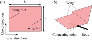
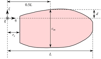
The wing–body model is composed of the same two wings and a body. The wing is infinitely thin and has a rectangular shape (see figure 1
a). The rectangular wing has length
 $L$
and width
 $c$
. We define the span direction along the length
 $L$
and the chord direction along the width
 $c$
. In this study, the aspect ratio, defined as the wing span squared divided by the wing area (e.g. Shyy et al.
Reference Shyy, Lian, Tang, Viieru and Liu2008),
 $AR=2L/c$
is set to 2, i.e.
 $L=c$
. We assume that the mass of the wing can be neglected, since in general the mass of actual insects’ wing is much smaller than that of their body. In order to neglect the effect of the wing flexibility, we assume that the wing is rigid.
Illustration of (a) a rectangular wing and (b) the wing–body model with two rectangular wings and a rod-shaped body.

The body is described as a straight infinitely thin rod with the length
 $L_{b}$
. We set
 $L_{b}=c$
for simplicity. The body has uniform (line) density
 ${\it\rho}_{b}$
. Therefore, the centre of mass (COM) of the body is at the middle point of the body and the total mass of the body is
 $M={\it\rho}_{b}L_{b}$
. The two wings are connected to the body in a manner such that the middle point of the wing root is located at that of the body (see figure 1
b).
2.2. Wing motion
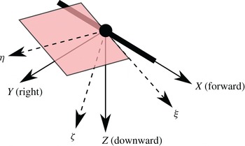
The wing motion relative to the body is described by the rotation of the coordinate system fixed to the wing relative to the body. First, we define the coordinate systems (see figure 2). Let the coordinate system fixed to the body be
 ${\it\Sigma}_{b}$
, and its origin be located at the COM of the body. The axes of
 ${\it\Sigma}_{b}$
are denoted by
 $X$
,
 $Y$
and
 $Z$
, where the
 $X$
-axis is parallel to the body. We define the forward direction relative to the body as the positive direction of the
 $X$
-axis, the right direction as the positive direction of the
 $Y$
-axis and the downward direction as the positive direction of the
 $Z$
-axis. Let the coordinate system fixed to the right wing be
 ${\it\Sigma}_{w}$
, and its origin be located at the middle point of the wing root. Therefore, the origin of
 ${\it\Sigma}_{w}$
is coincident with that of
 ${\it\Sigma}_{b}$
. The axes of
 ${\it\Sigma}_{w}$
are denoted by
 ${\it\xi}$
,
 ${\it\eta}$
and
 ${\it\zeta}$
, where the
 ${\it\xi}$
-axis is parallel to the chord direction and the
 ${\it\eta}$
-axis is parallel the span direction. Since the motion of the left wing is symmetrical to the right wing about the
 $Z{-}X$
plane, the definition of the coordinate system fixed to the left wing is not required.
Two axes fixed to the body (
 $X{-}Y{-}Z$
) and the right wing (
 ${\it\xi}{-}{\it\eta}{-}{\it\zeta}$
).

We describe the rotation of
 ${\it\Sigma}_{w}$
relative to
 ${\it\Sigma}_{b}$
by the 3–2–1 Euler angle. Let
 $\boldsymbol{e}_{X}$
,
 $\boldsymbol{e}_{Y}$
and
 $\boldsymbol{e}_{Z}$
be three unit vectors along the
 $X$
-,
 $Y$
- and
 $Z$
-axis, respectively, and
 $\boldsymbol{e}_{{\it\xi}}$
,
 $\boldsymbol{e}_{{\it\eta}}$
and
 $\boldsymbol{e}_{{\it\zeta}}$
be three unit vectors along the
 ${\it\xi}$
-,
 ${\it\eta}$
- and
 ${\it\zeta}$
-axis, respectively. The vector array
 $[\boldsymbol{e}_{{\it\xi}},\boldsymbol{e}_{{\it\eta}},\boldsymbol{e}_{{\it\zeta}}]$
is given by the successive orthogonal transformations of
 $[\boldsymbol{e}_{X},\boldsymbol{e}_{Y},\boldsymbol{e}_{Z}]$
as follows:
 $$\begin{eqnarray}[\boldsymbol{e}_{{\it\xi}},\boldsymbol{e}_{{\it\eta}},\boldsymbol{e}_{{\it\zeta}}]=[\boldsymbol{e}_{X},\boldsymbol{e}_{Y},\boldsymbol{e}_{Z}]\unicode[STIX]{x1D64E}_{3}(0)\unicode[STIX]{x1D64E}_{2}({\it\alpha}(t))\unicode[STIX]{x1D64E}_{1}(-{\it\theta}(t)),\end{eqnarray}$$
where
 $\unicode[STIX]{x1D64E}_{3}$
,
 $\unicode[STIX]{x1D64E}_{2}$
and
 $\unicode[STIX]{x1D64E}_{1}$
are the orthogonal matrices given by
 $$\begin{eqnarray}\displaystyle & \unicode[STIX]{x1D64E}_{3}({\it\phi})=\left[\begin{array}{@{}ccc@{}}\cos {\it\phi} & -\text{sin}{\it\phi} & 0\\ \sin {\it\phi} & \cos {\it\phi} & 0\\ 0 & 0 & 1\end{array}\right], & \displaystyle\end{eqnarray}$$
 $$\begin{eqnarray}\displaystyle & \unicode[STIX]{x1D64E}_{2}({\it\phi})=\left[\begin{array}{@{}ccc@{}}\cos {\it\phi} & 0 & \sin {\it\phi}\\ 0 & 1 & 0\\ -\text{sin}{\it\phi} & 0 & \cos {\it\phi}\end{array}\right], & \displaystyle\end{eqnarray}$$
 $$\begin{eqnarray}\displaystyle & \unicode[STIX]{x1D64E}_{1}({\it\phi})=\left[\begin{array}{@{}ccc@{}}1 & 0 & 0\\ 0 & \cos {\it\phi} & -\text{sin}{\it\phi}\\ 0 & \sin {\it\phi} & \cos {\it\phi}\end{array}\right]. & \displaystyle\end{eqnarray}$$
 ${\it\alpha}(t)$
and
 ${\it\theta}(t)$
in (2.1) are the angle of attack and the flapping angle at time
 $t$
, respectively, given by
 $$\begin{eqnarray}\displaystyle & \displaystyle {\it\alpha}(t)=\frac{{\it\alpha}_{m}}{2}\left[1+\cos \left(\frac{2{\rm\pi}}{T}t+{\it\gamma}\right)\right], & \displaystyle\end{eqnarray}$$
 $$\begin{eqnarray}\displaystyle & \displaystyle {\it\theta}(t)={\it\theta}_{m}\cos \left(\frac{2{\rm\pi}}{T}t\right), & \displaystyle\end{eqnarray}$$
 ${\it\alpha}_{m}$
is the maximum angle of attack,
 ${\it\theta}_{m}$
is the flapping amplitude corresponding to the half of the stroke amplitude,
 $T$
is the period of flapping motion and
 ${\it\gamma}$
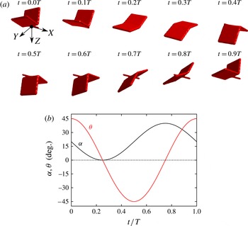
is the phase shift. In order to make a butterfly-like wing motion, we set
 ${\it\gamma}={\rm\pi}/2$
. Note that the wings are initially located at the most upward. In this study,
 ${\it\theta}_{m}$
is fixed to
 $45^{\circ }$
, and thus the wing motion is changed only by
 ${\it\alpha}_{m}$
. As an example, the wing motion with
 ${\it\alpha}_{m}=40^{\circ }$
is shown in figure 3.
(a) Illustration of the wing motion and (b) the time variations of the angle of attack
 ${\it\alpha}$
and the flapping angle
 ${\it\theta}$
with
 ${\it\alpha}_{m}=40^{\circ }$
during one stroke.

In this model, the stroke plane angle is changed by the angle of attack
 ${\it\alpha}(t)$
, which is the inclined angle of the wing root relative to the body. However, an actual butterfly changes the stroke plane angle by changing the angle of its body (as for the actual butterfly’s kinematics, see Sunada Reference Sunada1993; Huang & Sun Reference Huang and Sun2012; Yokoyama et al.
Reference Yokoyama, Senda, Iima and Hirai2013). Since the lift and thrust forces by the body motion are considered to be negligibly small, the difference between the present flapping and an actual butterfly flapping essentially gives no effect on estimating the forces generated by the flapping wings and the body.
3. Governing equations
We consider the motion of the butterfly-like flapping wing–body model in the Earth’s atmosphere and gravity. Since tiny insects move at low speed, the compressibility of the air can be neglected. Hence, we consider the incompressible Navier–Stokes equations for the fluid motion. The motion of the wing–body model is composed of the wing motion and the body motion. The wing motion is prescribed relative to the body as shown in the previous section. As mentioned above, the mass of the wings is neglected in the wing–body model, and the aerodynamic forces generated by the wings act on the body through the connecting point. The body motion is governed by the equation of motion with the aerodynamic forces and the gravitational force.
3.1. Fluid motion
The fluid motion around the wings and the body is governed by the incompressible Navier–Stokes equations as follows:
 $$\begin{eqnarray}\displaystyle & \displaystyle \boldsymbol{{\rm\nabla}}\boldsymbol{\cdot }\boldsymbol{u}=0, & \displaystyle\end{eqnarray}$$
 $$\begin{eqnarray}\displaystyle & \displaystyle \frac{\text{D}\boldsymbol{u}}{\text{D}t}=-\frac{1}{{\it\rho}_{f}}\boldsymbol{{\rm\nabla}}p+{\it\nu}{\rm\nabla}^{2}\boldsymbol{u}, & \displaystyle\end{eqnarray}$$
 $\boldsymbol{u}$
is the fluid velocity,
 $p$
is the pressure,
 ${\it\rho}_{f}$
is the density of the fluid and
 ${\it\nu}$
is the kinematic viscosity of the fluid. We consider the air at room temperature
 $20~^{\circ }\text{C}$
as the fluid, that is,
 ${\it\rho}_{f}=1.205~(\text{kg}~\text{m}^{-3})$
and
 ${\it\nu}=1.512\times 10^{-5}~(\text{m}^{2}~\text{s}^{-1})$
. It should be noted that the gravitational term is not appeared in (3.2). This is because the pressure
 $p$
includes the gravitational potential. The no-slip condition should be satisfied on the surface of the wing–body model, i.e. the fluid velocity must be equal to the velocity of the wings and the body.
In this study, we take the mean wing tip speed defined by
 $U_{tip}=4{\it\theta}_{m}L/T$
as the characteristic flow speed, and the wing length
 $L$
as the characteristic length. The governing parameter of the above equations is the Reynolds number
 $\mathit{Re}$
given by
 $$\begin{eqnarray}\mathit{Re}=\frac{U_{tip}L}{{\it\nu}}.\end{eqnarray}$$
It should be noted that another definition of the Reynolds number based on the mean wing chord length has been used for studying hovering flights conventionally (see Shyy et al. Reference Shyy, Lian, Tang, Viieru and Liu2008). On the other hand, several studies on butterfly’s flights (e.g. Ota et al. Reference Ota, Suzuki and Inamuro2012; Yokoyama et al. Reference Yokoyama, Senda, Iima and Hirai2013) have used the definition of the Reynolds number based on the wing length in the same way as (3.3).
3.2. Body motion
The body motion is described by the translational motion of the origin of
 ${\it\Sigma}_{b}$
and the rotational motion of
 ${\it\Sigma}_{b}$
relative to the coordinate system fixed to the space
 ${\it\Sigma}_{s}$
. The origin of
 ${\it\Sigma}_{b}$
, i.e. the COM of the body is denoted by
 $\boldsymbol{X}_{c}$
. In the following, vectors observed from
 ${\it\Sigma}_{b}$
have a pre-superscript
 $b$
, while vectors observed from
 ${\it\Sigma}_{s}$
have no pre-superscript. Let the axes of
 ${\it\Sigma}_{s}$
be
 $x$
,
 $y$
and
 $z$
and let
 $\boldsymbol{e}_{x}$
,
 $\boldsymbol{e}_{y}$
and
 $\boldsymbol{e}_{z}$
be three unit vectors along the axes, where the positive direction of the
 $y$
-axis is the upward direction. Therefore, the gravitational acceleration vector is given by
 $\boldsymbol{G}=-G\boldsymbol{e}_{y}$
where
 $G=9.807~(\text{m}~\text{s}^{-2})$
. The unit vectors
 $\boldsymbol{e}_{X}$
and
 $\boldsymbol{e}_{Z}$
of
 ${\it\Sigma}_{b}$
are initially coincident with
 $\boldsymbol{e}_{x}$
and
 $-\boldsymbol{e}_{y}$
of
 ${\it\Sigma}_{s}$
, respectively. The vector array
 $[\boldsymbol{e}_{X},\boldsymbol{e}_{Y},\boldsymbol{e}_{Z}]$
is given by an orthogonal transformation of
 $[\boldsymbol{e}_{x},\boldsymbol{e}_{y},\boldsymbol{e}_{z}]$
as follows:
 $$\begin{eqnarray}[\boldsymbol{e}_{X},\boldsymbol{e}_{Y},\boldsymbol{e}_{Z}]=[\boldsymbol{e}_{x},\boldsymbol{e}_{y},\boldsymbol{e}_{z}]\unicode[STIX]{x1D64E}(\boldsymbol{Q}(t)),\end{eqnarray}$$
where
 $\unicode[STIX]{x1D64E}(\boldsymbol{Q})$
is an orthogonal matrix represented by a unit quaternion
 $\boldsymbol{Q}=(q_{0},q_{1},q_{2},q_{3})^{\text{T}}$
(where the superscript T represents the transpose of a vector or a matrix). The detail of the quaternion and the kinematic equations of the body are shown in appendix A.
Let
 $\boldsymbol{U}_{c}(t)$
be the velocity of
 $\boldsymbol{X}_{c}(t)$
and
 $~^{b}{\it\bf\Omega}_{c}(t)$
be the angular velocity of the body. Supposing that we obtain the total aerodynamic force
 $\boldsymbol{F}_{aero}(t)$
generated by the wings and the body and the total aerodynamic torque
 $\boldsymbol{T}_{aero}(t)$
around
 $\boldsymbol{X}_{c}(t)$
,
 $\boldsymbol{U}_{c}(t)$
and
 $~^{b}{\it\bf\Omega}_{c}(t)$
are governed by the Newton–Euler equations as follows:
 $$\begin{eqnarray}\displaystyle & M\displaystyle \frac{\text{d}\boldsymbol{U}_{c}}{\text{d}t}=\boldsymbol{F}_{aero}+M\boldsymbol{G}, & \displaystyle\end{eqnarray}$$
 $$\begin{eqnarray}\displaystyle & \displaystyle \unicode[STIX]{x1D644}_{b}\frac{\text{d}^{b}{\it\bf\Omega}_{c}}{\text{d}t}+^{b}{\it\bf\Omega}_{c}\times (\unicode[STIX]{x1D644}_{b}\text{ }^{b}{\it\bf\Omega}_{c})=\unicode[STIX]{x1D64E}(\boldsymbol{Q})^{\text{T}}\boldsymbol{T}_{aero}. & \displaystyle\end{eqnarray}$$
 $\unicode[STIX]{x1D644}_{b}$
is the inertia matrix observed in
 ${\it\Sigma}_{b}$
given by
 $$\begin{eqnarray}\unicode[STIX]{x1D644}_{b}=\left[\begin{array}{@{}ccc@{}}0 & 0 & 0\\ 0 & \frac{1}{12}ML_{b}^{2} & 0\\ 0 & 0 & \frac{1}{12}ML_{b}^{2}\end{array}\right].\end{eqnarray}$$
Note that in the present wing–body model the mass of the wings is neglected. It should be noted that the components of the first row of
 $\unicode[STIX]{x1D644}_{b}$
are all zero. This is because the body of the present wing–body model is an infinitely thin rod, i.e. the moment of inertia about the axis parallel to the body (the
 $X$
-axis) is zero. So, we cannot consider the rotation about the
 $X$
-axis, which corresponds to the roll motion. In this study, we neglect the roll motion, but consider the pitch motion (the rotation about the
 $Y$
-axis) and the yaw motion (the rotation about the
 $Z$
-axis). Therefore, the motion of the wing–body model has 3 degrees of freedom (DOFs) in the translational motion and 2 DOFs in the rotational motion, i.e. 5 DOFs in total. Note that the buoyancy force is not included in (3.5), since the wing–body model has no volume.
The governing parameters of (3.5) and (3.6) are the non-dimensional mass
 $N_{M}$
and the Froude number
 $\mathit{Fr}$
defined as
 $$\begin{eqnarray}\displaystyle & \displaystyle N_{M}=\frac{M}{{\it\rho}_{f}L^{3}}, & \displaystyle\end{eqnarray}$$
 $$\begin{eqnarray}\displaystyle & \displaystyle Fr=\frac{U_{tip}}{\sqrt{LG}}. & \displaystyle\end{eqnarray}$$
 $\unicode[STIX]{x1D649}_{I}$
is determined by
 $N_{M}$
in the wing–body model as follows:
 $$\begin{eqnarray}\unicode[STIX]{x1D649}_{I}=\frac{\unicode[STIX]{x1D644}_{b}}{{\it\rho}_{f}L^{5}}=\left[\begin{array}{@{}ccc@{}}0 & 0 & 0\\ 0 & \frac{1}{12}N_{M} & 0\\ 0 & 0 & \frac{1}{12}N_{M}\end{array}\right].\end{eqnarray}$$
3.3. Governing parameters and degrees of freedom
As shown in §§ 3.1 and 3.2, the governing parameters of the system are the Reynolds number
 $\mathit{Re}$
, the non-dimensional mass
 $N_{M}$
and the Froude number
 $\mathit{Fr}$
. In order to calculate free flights of the wing–body model in fluid, we have to determine the three parameters. However, the three parameters are not determined independently. Actually, the relation between
 $\mathit{Re}$
and
 $\mathit{Fr}$
is given by
 $$\begin{eqnarray}\frac{Fr}{\mathit{Re}}=\frac{{\it\nu}}{\sqrt{L^{3}G}}.\end{eqnarray}$$
Being given the values of
 ${\it\nu}$
and
 $G$
in the Earth’s atmosphere and gravity, the ratio of
 $\mathit{Fr}$
to
 $\mathit{Re}$
is determined by setting the wing length
 $L$
. Therefore, the wing length
 $L$
can be treated as equivalent to the ratio of the Reynolds number to the Froude number in this situation.
It should be noted that in this study the Strouhal number does not appear as a governing parameter unlike many other studies on flapping wings (e.g. Triantafyllou, Triantafyllou & Grosenbaugh Reference Triantafyllou, Triantafyllou and Grosenbaugh1993; Wang Reference Wang2000; Taylor, Nudds & Thomas Reference Taylor, Nudds and Thomas2003). The Strouhal number is defined by
 $\mathit{St}=F_{req}L_{ref}/U_{ref}$
where
 $F_{req}$
is the flapping frequency,
 $L_{ref}$
is the characteristic length and
 $U_{ref}$
is the characteristic velocity. In general, the stroke amplitude and the forward velocity are chosen as
 $L_{ref}$
and
 $U_{ref}$
, respectively (e.g. Shyy et al.
Reference Shyy, Lian, Tang, Viieru and Liu2008). The Strouhal number is an important governing parameter when the forward velocity is chosen as the characteristic velocity. In this study, however, we use the flapping velocity as the characteristic velocity. Therefore, the Strouhal number is not included in governing parameters here. For the same reason, the reduced frequency (see Shyy et al.
Reference Shyy, Lian, Tang, Viieru and Liu2008, Reference Shyy, Aono, Chimakurthi, Trizila, Kang, Cesnik and Liu2010) does not appear as a governing parameter. Although we can calculate the Strouhal number by using the forward velocity obtained as a result of a free flight, it is not a parameter but a result. The resulting Strouhal number can be seen in § 5.2.2.
In this study, the following four kinds of simulations are carried out: (i) the computation of aerodynamic forces; (ii) free flight (without rotation) simulations; (iii) free flight (with rotation) simulations; and (iv) the computation for controlling the rotational motion. In the simulation (i), we neglect (3.5) and (3.6). Hence, the motion of the wing–body model has 0 DOFs and the governing parameter of the system is only
 $\mathit{Re}$
. In the simulation (ii), we calculate (3.5) for the translational motion, but neglect (3.6) for the rotational motion. Thus, the motion of the wing–body model has 3 DOFs and the governing parameters of the system are
 $\mathit{Re}$
,
 $N_{M}$
and
 $\mathit{Fr}$
. In the simulation (iii), we calculate both (3.5) and (3.6), that is, the motion of the wing–body model has 5 DOFs and the governing parameters of the system are
 $\mathit{Re}$
,
 $N_{M}$
and
 $\mathit{Fr}$
. In the simulation (iv), we calculate Lagrange equations for the thorax–abdomen system (see § 5.4) instead of (3.5) and (3.6), while the governing parameters of the system are
 $\mathit{Re}$
,
 $N_{M}$
and
 $\mathit{Fr}$
.
4. Computational conditions
We use the IB-LBM (Suzuki & Inamuro Reference Suzuki and Inamuro2011) for solving (3.1) and (3.2). The motion of the body determined by (A 3), (A 4), (3.5) and (3.6) is computed by the second-order Adams–Bashforth method. In calculating the aerodynamic force and torque, the internal mass effect (see Suzuki & Inamuro Reference Suzuki and Inamuro2011) is neglected, since the wing–body model has no volume. It should be noted that in this study we take into account the aerodynamic force and torque acting on not only the wings but also the body. However, in our preliminary calculations, the aerodynamic force and torque acting on the body are two orders of magnitude smaller than those acting on the wings. Although the aerodynamic force and torque acting on the body can be neglected, we take them into account in this study. For the details of the numerical method, see Suzuki & Inamuro (Reference Suzuki and Inamuro2011). Validations of the numerical method are described in appendix B.
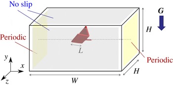
The computational domain is a cuboid with width
 $W$
, height
 $H$
and depth
 $H$
as shown in figure 4. The boundary condition on two sides perpendicular to the
 $x$
-axis is the periodic boundary condition, and on the other sides the no-slip condition is used. This computational condition corresponds to the situation where the wing–body models are placed at regular intervals of
 $W$
. If the interval
 $W$
is much larger than the wing length
 $L$
, the effect of the neighboring models can be neglected. The COM of the body is initially placed at the centre of the domain filled with a stationary fluid at uniform pressure.
Computational domain for simulations of flows around the butterfly-like flapping wing–body model.

In the following calculations, we use a moving multi-block grid (Inamuro Reference Inamuro2012) in order to save computation time. The multi-block grid is composed of a moving fine grid with a lattice spacing
 ${\rm\Delta}x$
and a stationary coarse grid with
 $2{\rm\Delta}x$
. The moving fine grid is used only around the wing–body model, and the stationary coarse grid is used in the other domain. For the fine grid, we use an inner cubic domain with width
 $D$
which moves together with the motion of the body. The centre of the inner domain is initially placed at the COM of the body.
The simulation (i) is performed in the domain of
 $W=12L$
,
 $H=6L$
and
 $D=3L$
for
 $50\leqslant \mathit{Re}\leqslant 1000$
, while the simulations (ii)–(iv) are performed in the domain of
 $W=12L$
,
 $H=12L$
, and
 $D=2.4L$
for various Reynolds numbers of
 $\mathit{Re}<1200$
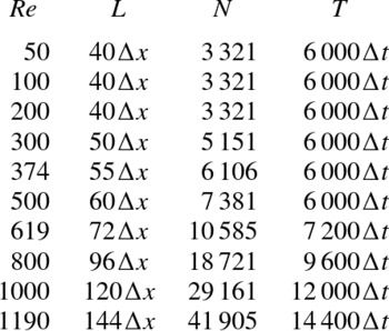
. The spatial and temporal resolutions for each
 $\mathit{Re}$
are shown in table 1. The dependence of grid resolution is examined in appendix C. In order to save the computational cost for
 $\mathit{Re}>500$
, we calculate one-half of the computational domain with the mirror boundary condition on the longitudinal plane which passes through the centre of the domain and is perpendicular to
 $z$
-axis. This implies that the flow field is assumed to be symmetrical with respect to the longitudinal plane, and the body is assumed to move only in the longitudinal plane, i.e. the translational velocity and the angular velocity are restricted to
 $\boldsymbol{U}_{c}=(U_{x},U_{y},0)^{\text{T}}$
and
 $~^{b}{\it\bf\Omega}_{c}=(0,{\it\omega}_{2},0)^{\text{T}}$
, respectively. It should be noted that for
 $\mathit{Re}\leqslant 500$
we calculate the whole of the computational domain and do not use the above assumption.
Spatial and temporal resolutions. The total number of boundary Lagrangian points
 $N$
includes that of the body, the right wing and the left wing. Here
 ${\rm\Delta}x$
is the lattice spacing and
 ${\rm\Delta}t$
is the time step.

5. Results and discussion
5.1. Computation of aerodynamic forces for fixed body
5.1.1. Induced flows by the wing–body model
First, we calculate flows around the wing–body model with
 ${\it\alpha}_{m}=40^{\circ }$
,
 $60^{\circ }$
and
 $90^{\circ }$
for the Reynolds numbers of
 $50\leqslant \mathit{Re}\leqslant 1000$
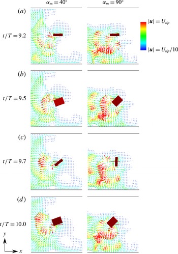
, when the body is fixed. Figure 5 shows the velocity fields projected onto
 $x{-}y$
plane during the 10th stroke for
 $\mathit{Re}=500$
. We can see from figure 5 that the wing–body model induces a backward flow and a downward flow during one stroke. It can be expected that both mean lift and thrust forces are induced as reactions to the induced flows. Ota et al. (Reference Ota, Suzuki and Inamuro2012) and Kimura et al. (Reference Kimura, Suzuki and Inamuro2014) reported that the symmetry breaking occurs with respect to the longitudinal plane in the two-dimensional symmetric flapping wings. However, in all results for
 $\mathit{Re}\leqslant 500$
of this study, the flow field is symmetrical with respect to the longitudinal plane.
Velocity fields around the wing–body model with
 ${\it\alpha}_{m}=40^{\circ }$
and
 $90^{\circ }$
at
 $t/T=9.2$
, 9.5, 9.7 and 10.0 for
 $\mathit{Re}=500$
projected onto the
 $x{-}y$
plane when the body is fixed. The wing–body model is shown as a red surface. The colours of vectors denote the magnitude of the velocity vectors. The velocity vectors are drawn at every
 $10{\rm\Delta}x$
.

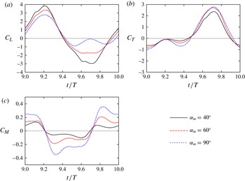
Time variations of (a) lift coefficient
 $C_{L}$
, (b) thrust coefficient
 $C_{T}$
and (c) pitching moment coefficient
 $C_{M}$
with
 ${\it\alpha}_{m}=40^{\circ }$
,
 $60^{\circ }$
and
 $90^{\circ }$
for
 $\mathit{Re}=500$
.

5.1.2. Aerodynamic forces and pitching moment
Next, we show the aerodynamic forces and pitching moment. We define the lift coefficient
 $C_{L}$
, the thrust coefficient
 $C_{T}$
and the pitching moment coefficient
 $C_{M}$
as follows:
 $$\begin{eqnarray}\displaystyle & \displaystyle C_{L}=\frac{\boldsymbol{F}_{aero}\boldsymbol{\cdot }\boldsymbol{e}_{y}}{0.5{\it\rho}_{f}U_{tip}^{2}(2L\,c)}, & \displaystyle\end{eqnarray}$$
 $$\begin{eqnarray}\displaystyle & \displaystyle C_{T}=\frac{\boldsymbol{F}_{aero}\boldsymbol{\cdot }\boldsymbol{e}_{x}}{0.5{\it\rho}_{f}U_{tip}^{2}(2L\,c)}, & \displaystyle\end{eqnarray}$$
 $$\begin{eqnarray}\displaystyle & \displaystyle C_{M}=\frac{\boldsymbol{T}_{aero}\boldsymbol{\cdot }\boldsymbol{e}_{z}}{0.5{\it\rho}_{f}U_{tip}^{2}(2L\,c)L}. & \displaystyle\end{eqnarray}$$
 ${\it\Sigma}_{s}$
. Figure 6 shows the time variations of
 $C_{L}$
,
 $C_{T}$
and
 $C_{M}$
with
 ${\it\alpha}_{m}=40^{\circ }$
,
 $60^{\circ }$
and
 $90^{\circ }$
for
 $\mathit{Re}=500$
in one stroke of
 $9.0\leqslant t/T\leqslant 10.0$
. The simulations are conducted until
 $t=20T$
, but the results during each stroke are almost the same after
 $t=9T$
. Thus, we present the results of tenth period here. It can be seen from figure 6(a) that
 $C_{L}$
reaches its positive peak around
 $t/T=9.2$
for all
 ${\it\alpha}_{m}$
, while the negative peak of
 $C_{L}$
is around
 $t/T=9.7$
for
 ${\it\alpha}_{m}=40^{\circ }$
and
 $60^{\circ }$
and around
 $t/T=9.5$
for
 ${\it\alpha}_{m}=90^{\circ }$
. The magnitude of the negative peak decreases significantly as
 ${\it\alpha}_{m}$
increases. Note that the magnitude of the positive peak is larger than that of the negative peak for all
 ${\it\alpha}_{m}$
. On the other hand, it can be seen from figure 6(b) that
 $C_{T}$
reaches its negative peak around
 $t/T=9.0$
and its positive peak around
 $t/T=9.7$
for all
 ${\it\alpha}_{m}$
. Also, the magnitude of the positive peak is much larger than that of the negative peak. In comparing 6(a,b), we can see that the thrust coefficient looks very asymmetrical as compared with the lift coefficient. This is because the angle of attack
 ${\it\alpha}$
changes asymmetrically (
 $0\leqslant {\it\alpha}\leqslant {\it\alpha}_{m}$
), while the flapping angle
 ${\it\theta}$
changes symmetrically (
 $-{\it\theta}_{m}\leqslant {\it\theta}\leqslant {\it\theta}_{m}$
) as shown in figure 3(b). Since the thrust force is induced by the attacking motion (if
 ${\it\alpha}_{m}=0$
, no thrust force is induced), the thrust coefficient changes asymmetrically compared with the lift coefficient. It should be noted that the lift coefficient in figure 6(a) is rather different from that of figure 24 in § B.2. This is because the wing motions are considerably different, that is, one is for a forward flight of a butterfly and the other is for a hovering of an insect. From figure 6(c), we can see that the curve of
 $C_{M}$
has a shape similar to a square wave which is negative in
 $9.2\leqslant t/T\leqslant 9.7$
and positive in the other duration. The magnitude of the positive peak is almost equal to that of the negative peak for all
 ${\it\alpha}_{m}$
. Actually, the mean value of
 $C_{M}$
is more than two orders of magnitude smaller than the magnitude of the peak value. This means that the COM of the body is almost coincident with the mean centre of pressure. The magnitude of the peak value of
 $C_{M}$
increases as
 ${\it\alpha}_{m}$
increases.
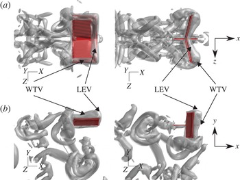
Vortical structures visualized by the
 $Q$
-criterion, that is, the second invariant of velocity gradient tensor at
 $t/T=9.2$
and 9.7 with
 ${\it\alpha}_{m}=90^{\circ }$
for
 $\mathit{Re}=500$
viewed from (a) the top side and (b) the right side of the wing–body model when the body is fixed. The wing–body model is shown as a red surface, and the isosurface of
 $Q=3(U_{tip}/L)^{2}$
is shown as a grey surface.

Figure 7 shows the vortical structures near the wing–body model with
 ${\it\alpha}_{m}=90^{\circ }$
for
 $\mathit{Re}=500$
at
 $t/T=9.2$
and 9.7. It should be noted that the lift coefficient reaches its positive peak around
 $t/T=9.2$
and the thrust coefficient reaches its positive peak around
 $t/T=9.7$
. The low-pressure vortices structures are identified by the
 $Q$
-criterion (Hunt, Wray & Moin Reference Hunt, Wray and Moin1988), i.e. the second invariant of the velocity gradient tensor given by
 $$\begin{eqnarray}Q=-\frac{\partial u_{i}}{\partial x_{j}}\frac{\partial u_{j}}{\partial x_{i}}\end{eqnarray}$$
where
 $i,j=x,y,z$
represent the Cartesian coordinates and the summation convention is used. It can be seen from figure 7 that a wing-tip vortex (WTV) and a leading-edge vortex (LEV) appear on the upper surface of the wings at
 $t/T=9.2$
and on the lower surface of the wings at
 $t/T=9.7$
. Like an actual butterfly (Yokoyama et al.
Reference Yokoyama, Senda, Iima and Hirai2013), the WTV and the LEV are considered to be a main cause of the lift and thrust generation of the present wing–body model. Also, the LEV on the left wing is connected continuously to that on the right wing. The same feature is shown in the flow visualization around free-flying butterflies conducted by Srygley & Thomas (Reference Srygley and Thomas2002) and is distinctive from the experiments using fruit fly and hawkmoth wings (e.g. Ellington et al.
Reference Ellington, van den Berg, Willmott and Thomas1996; Birch, Dickson & Dickinson Reference Birch, Dickson and Dickinson2004). Srygley & Thomas (Reference Srygley and Thomas2002) also reported that the structure of the wake behind the butterfly is broken by the wings when the wing–wake interaction occurs. However, we cannot observe from figure 7 that the structure of the wake behind the model is broken. It should be noted that in the experiment by Srygley & Thomas (Reference Srygley and Thomas2002) the case where the wing–wake interaction does not occur is also observed. Therefore, our results are not inconsistent with an actual butterfly. Instead, it can be seen from figure 7 that the WTV and the LEV at downstroke and upstroke are released downward and backward, respectively, and form a vortex ring. The vortex ring is observed also in the free flight simulation of a butterfly by Huang & Sun (Reference Huang and Sun2012).
As for lift generation, it has been reported in Iima & Yanagita (Reference Iima and Yanagita2001) and Ota et al. (Reference Ota, Suzuki and Inamuro2012) that for a two-dimensional symmetric flapping wing the symmetry breaking of flows generates a mean lift force. The two-dimensional symmetric flapping wing corresponds to the present wing–body model with
 $c\rightarrow \infty$
and
 ${\it\alpha}_{m}=0^{\circ }$
. However, in our preliminary calculations using the present model with
 $c=L$
and
 ${\it\alpha}_{m}=0^{\circ }$
, the symmetry breaking of flows does not appear, and no mean lift force is generated for
 $\mathit{Re}\leqslant 1000$
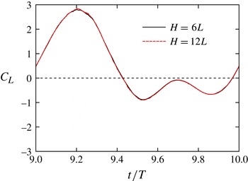
. This is because the vorticity in the three-dimensional flow field is completely different from that in the two-dimensional flow field. As another possibility for the lift generation, one might consider a ground effect (Gao & Lu Reference Gao and Lu2008). Indeed, in figure 5 the flow velocities reach the ground. In order to evaluate the ground effect, we performed the same simulation in a wider computational domain of
 $W=H=12L$
with
 ${\it\alpha}_{m}=90^{\circ }$
for
 $\mathit{Re}=500$
. It can be seen from figure 8 that the lift coefficient obtained in the wider domain of
 $H=12L$
is almost coincident with that in the standard domain of
 $H=6L$
. This means that the ground effect is not important in the present simulations.
Comparison of the lift coefficient between the wider computational domain of
 $H=12L$
and the standard domain of
 $H=6L$
with
 ${\it\alpha}_{m}=90^{\circ }$
for
 $\mathit{Re}=500$
.

Time variations of (a) lift coefficient
 $C_{L}$
, (b) thrust coefficient
 $C_{T}$
and (c) power coefficient
 $C_{P}$
with
 ${\it\alpha}_{m}=90^{\circ }$
for
 $\mathit{Re}=50$
, 100, 500 and 1000.

5.1.3. Aerodynamic performance
Here we investigate the aerodynamic performance by calculating the time-averaged aerodynamic forces, the power and the efficiency. We define the power coefficient
 $C_{P}$
as follows:
 $$\begin{eqnarray}C_{P}=\frac{\mathop{\sum }_{wing}\boldsymbol{f}_{local}\boldsymbol{\cdot }\boldsymbol{u}_{local}}{0.5{\it\rho}_{f}U_{tip}^{3}(2L\,c)},\end{eqnarray}$$
where
 $\sum _{wing}$
means the summation over Lagrangian points on the wings,
 $\boldsymbol{f}_{local}$
is the force locally acting on the fluid at a Lagrangian point on the wings and
 $\boldsymbol{u}_{local}$
is the flow velocity at the point. Therefore,
 $\sum _{wing}\boldsymbol{f}_{local}\boldsymbol{\cdot }\boldsymbol{u}_{local}$
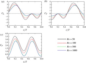
represents the power expended in moving the wings against the aerodynamic forces. At first, we show the time variations of the lift, thrust and power coefficients with
 ${\it\alpha}_{m}=90^{\circ }$
for various Reynolds numbers. In comparing the lift coefficients for
 $\mathit{Re}=50$
and 100 in figure 9(a), it can be seen that both positive and negative peaks much decrease to the same degree as the Reynolds number increases. This is because for low Reynolds numbers the wings receive a large viscous resistance. For
 $\mathit{Re}\geqslant 100$
, the magnitude of the positive peak of
 $C_{L}$
slightly decreases as the Reynolds number increases, while the magnitude of the negative peaks much decrease as the Reynolds number increases. Therefore, the time-averaged lift coefficient is expected to increase as the Reynolds number increases. Since the positive peak of
 $C_{L}$
is caused mainly by the LEV and the WTV at downstroke, it can be expected that the LEV and the WTV at downstroke do not change so much for
 $100\leqslant \mathit{Re}\leqslant 1000$
. Actually, in our preliminary calculations, the LEV and the WTV at downstroke are not so different between
 $\mathit{Re}=100$
and
 $500$
. On the other hand, since the negative peaks appear when the projected area of the wings onto the horizontal plane is relatively small, the shear stress, i.e. the viscous skin friction has a large contribution on the negative peaks of the lift coefficient. Therefore, the decrease in the viscous skin friction with the Reynolds number is considered as a main cause of the decrease in the magnitude of the negative peaks. We can see from figure 9(b) that the thrust coefficient has the same feature as the lift coefficient, although the phase of the thrust coefficient differs by
 $T/2$
compared with the lift coefficient. Since the model with
 ${\it\alpha}_{m}=90^{\circ }$
flaps downward in the downstroke and directly backward in the upstroke, the roles of the downstroke and the upstroke in the lift coefficient are replaced by the upstroke and the downstroke in the thrust coefficient, respectively. In addition, it can be seen from figure 9(c) that the power coefficient totally decreases as the Reynolds number increases. Consequently, the decrease in the power coefficient is presumably due to the decrease in the viscous skin friction.
The time-averaged values of
 $C_{L}$
,
 $C_{T}$
and
 $C_{P}$
are important indices of the aerodynamic performance. Let
 $\overline{C_{L}}$
,
 $\overline{C_{T}}$
and
 $\overline{C_{P}}$
be the time-averaged values in the 10th stroke (
 $9\leqslant t/T\leqslant 10$
). In addition, we define the efficiency by
 $$\begin{eqnarray}E_{ff}=\frac{\sqrt{\overline{C_{L}}^{2}+\overline{C_{T}}^{2}}}{\overline{C_{P}}}.\end{eqnarray}$$
It should be noted that Zheng, Hedrick & Mittal (Reference Zheng, Hedrick and Mittal2013) use the ratio of the lift coefficient to the power coefficient as an efficiency, which is a similar definition to that in this study. Since in this study the model generates the thrust force as well as the lift force, the ratio of the magnitude of the vector
 $(\overline{C_{T}},\overline{C_{L}})$
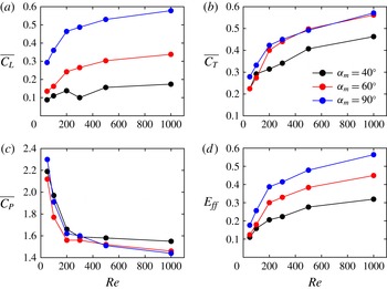
to the power coefficient seems more appropriate for the definition of the efficiency. Figure 10 shows
 $\overline{C_{L}}$
,
 $\overline{C_{T}}$
,
 $\overline{C_{P}}$
and
 $E_{ff}$
against various Reynolds numbers for
 ${\it\alpha}_{m}=40^{\circ }$
,
 $60^{\circ }$
and
 $90^{\circ }$
. It can be seen from figure 10(a,b) that both
 $\overline{C_{L}}$
and
 $\overline{C_{T}}$
increase as
 ${\it\alpha}_{m}$
and
 $\mathit{Re}$
increase. However, the rate of increasing both in
 $\overline{C_{L}}$
and
 $\overline{C_{T}}$
against
 $\mathit{Re}$
becomes smaller as
 $\mathit{Re}$
increases. From figure 10(c), we can see that
 $\overline{C_{P}}$
decreases as
 $\mathit{Re}$
increases, while it varies only slightly as
 ${\it\alpha}_{m}$
changes. It can be seen from figure 10(d) that
 $E_{ff}$
increases as
 ${\it\alpha}_{m}$
and
 $\mathit{Re}$
increase. This means that the wing–body model can generate larger lift and thrust forces by a smaller power as
 ${\it\alpha}_{m}$
and
 $\mathit{Re}$
increase. These results are consistent with earlier findings (e.g. Wu & Sun Reference Wu and Sun2004; Lentink & Dickinson Reference Lentink and Dickinson2009; Zheng et al.
Reference Zheng, Hedrick and Mittal2013).
The time-averaged (a) lift coefficient
 $\overline{C_{L}}$
, (b) thrust coefficient
 $\overline{C_{T}}$
and (c) power coefficient
 $\overline{C_{P}}$
, and (d) the efficiency
 $E_{ff}$
against various Reynolds numbers for
 ${\it\alpha}_{m}=40^{\circ }$
,
 $60^{\circ }$
and
 $90^{\circ }$
.

5.1.4. Expected supportable mass
Finally, we estimate the supportable mass by using
 $\overline{C_{L}}$
shown in figure 10(a). Letting the wing–body model have a mass of
 $M_{exp}$
, the gravitational force acting on the wing–body model
 $M_{exp}G$
should be balanced by the time-averaged lift force
 $\overline{\boldsymbol{F}_{aero}}\boldsymbol{\cdot }\boldsymbol{e}_{y}$
for supporting the mass. Hereafter,
 $M_{exp}$
is called the expected supportable mass. The non-dimensional expected supportable mass
 $N_{Mexp}$
can be calculated by using (3.8) and (5.1) as follows:
 $$\begin{eqnarray}N_{Mexp}=\frac{c}{L}\frac{U_{tip}^{2}}{LG}\overline{C_{L}}=\frac{2}{AR}\left(\frac{\mathit{Fr}}{\mathit{Re}}\right)^{2}\mathit{Re}^{2}\overline{C_{L}}.\end{eqnarray}$$
In the right-hand side of (5.7), the ratio
 $\mathit{Fr}/\mathit{Re}$
is determined by setting the wing length
 $L$
in (3.11). In addition,
 $\overline{C_{L}}$
is given against
 $\mathit{Re}$
for each
 ${\it\alpha}_{m}$
in figure 10(a). Therefore,
 $N_{Mexp}$
can be obtained against
 $\mathit{Re}$
for each
 ${\it\alpha}_{m}$
and
 $L$
.
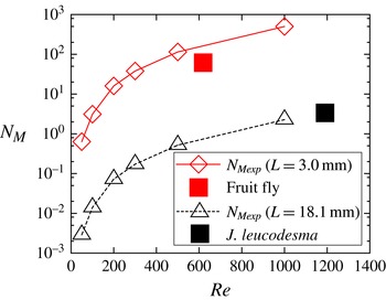
Figure 11 shows the non-dimensional expected supportable mass against
 $\mathit{Re}$
for
 ${\it\alpha}_{m}=90^{\circ }$
with
 $L=3.0$
and 18.1 mm. The figure includes the two curves for the scale of a fruit fly (Drosophila melanogaster,
 $L=3.0~\text{mm}$
) and for the scale of a small butterfly (Janatella leucodesma,
 $L=18~\text{mm}$
). It can be expected that a smaller mass than
 $N_{Mexp}$
can be supported by the lift force against the gravity, while a larger mass cannot be supported by the lift force. The actual parameters of a fruit fly and a J. leucodesma are listed in table 2, and the non-dimensional parameters are plotted in figure 11. It can be seen from figure 11 that the parameter of a fruit fly is under the curve of
 $N_{Mexp}$
for
 $L=3.0~\text{mm}$
, and the parameter of a J. leucodesma is found along an extension of the curve of
 $N_{Mexp}$
for
 $L=18.1~\text{mm}$
. Therefore, we can expect that the present wing–body model has a similar aerodynamic performance to actual insects.
The non-dimensional expected supportable mass against various Reynolds numbers for
 ${\it\alpha}_{m}=90^{\circ }$
. The upper (red online) curve describes
 $N_{Mexp}$
for
 $L=3.0~\text{mm}$
, and the lower (black) curve for
 $L=18.1~\text{mm}$
. The conditions for a fruit fly (
 $L=3.0~\text{mm}$
) and a small butterfly (
 $L=18.1~\text{mm}$
) are also included.

Trajectories of the COM of the wing–body model with
 $N_{M}=16$
, 17, 20 and 30 for
 $\mathit{Re}=200$
. The initial position of the COM (the centre of the domain) is denoted by
 $(x/L,y/L)=(0,0)$
. The symbols on the trajectories indicate the position of the COM when the wings are at top dead point.

Flight parameters for a fruit fly and a J. leucodesma. Four dimensional parameters (the wing length
 $L$
, the flapping frequency
 $F_{req}=1/T$
, the mean wing tip speed
 $U_{tip}$
and the mass
 $M$
) and three non-dimensional parameters (the Reynolds number
 $\mathit{Re}$
, the Froude number
 $\mathit{Fr}$
and the non-dimensional mass
 $N_{M}$
) are specified. It should be noted that the Reynolds number is based on the mean wing tip speed and the wing length, while that for a fruit fly is conventionally based on the velocity of the chord section and the wing chord length.

5.2. Free flight (without rotation) simulation
Since the expected supportable mass is estimated by using the lift force when the body is fixed, the following question is not trivial: Can the expected supportable mass actually be supported in a free flight? In order to answer the above question, we simulate free flights by the wing–body model when the body can move translationally but cannot rotate. In this simulation, we set
 ${\it\alpha}_{m}=90^{\circ }$
since the aerodynamic performance for
 ${\it\alpha}_{m}=90^{\circ }$
is the best in the results shown in § 5.1.3. In the following, we show two kinds of simulations: the cases for
 $L=3.0~\text{mm}$
and for
 $L=18.1~\text{mm}$
. From (3.11), the ratio
 $\mathit{Fr}/\mathit{Re}$
is fixed to be
 $2.9\times 10^{-2}$
and
 $1.98\times 10^{-3}$
for
 $L=3.0~\text{mm}$
and for
 $L=18.1~\text{mm}$
, respectively. Note that in all of the results of these simulations the flow field is symmetrical with respect to the longitudinal plane and
 $\boldsymbol{U}_{c}=(U_{x},U_{y},0)^{\text{T}}$
, while no assumption about the flow field and the body motion is used for
 $\mathit{Re}\leqslant 500$
(see § 4).
5.2.1. Case for
 $L=3.0~\text{mm}$

Figure 12 shows the trajectories of the COM of the wing–body model with
 $N_{M}=16$
, 17, 20 and 30 (in the dimensional mass,
 $M=0.521$
, 0.553, 0.651 and 0.976 mg, respectively) for
 $\mathit{Re}=200$
in the case of
 $L=3.0~\text{mm}$
. It should be noted that
 $N_{M}=16$
is equal to the non-dimensional expected supportable mass
 $N_{Mexp}$
for
 $\mathit{Re}=200$
. It can be seen from figure 12 that the wing–body model with
 $N_{M}=N_{Mexp}$
can go upward against the gravity. In addition, the wing–body model with
 $N_{M}=17>N_{Mexp}$
can also go upward, while the model with
 $N_{M}=30$
goes downward. It is interesting that the model with
 $N_{M}=20$
goes slightly downward at first, and then keeps at a steady altitude. This is because the lift force increases as the forward speed of the model increases.
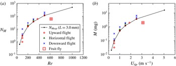
By calculating free flights for various Reynolds numbers and non-dimensional masses, we can obtain the conditions for upward flights, downward flights and almost horizontal flights. The results are shown in figure 13(a) which also includes the non-dimensional expected supportable mass
 $N_{Mexp}$
. From this figure, it can be seen that the boundary between points for upward flight and those for downward flight is consistent with the curve of
 $N_{Mexp}$
. In particular, it is found that the present wing–body model with the same condition as a fruit fly can go upward against the gravity. This means that even a simple wing–body model can generate enough lift force to support actual insects’ weight for
 $L=3.0~\text{mm}$
. Figure 13(b) shows the map of
 $U_{tip}{-}M$
which is equivalent to the map of
 $\mathit{Re}{-}N_{M}$
in figure 13(a) but described by the dimensional variables of the mean wing tip speed
 $U_{tip}$
and the mass
 $M$
which are related to
 $\mathit{Re}$
and
 $N_{M}$
as follows:
 $$\begin{eqnarray}\displaystyle & \displaystyle U_{tip}=\frac{{\it\nu}}{L}\mathit{Re}, & \displaystyle\end{eqnarray}$$
 $$\begin{eqnarray}\displaystyle & M={\it\rho}_{f}L^{3}N_{M}. & \displaystyle\end{eqnarray}$$
The map of (a)
 $\mathit{Re}{-}N_{M}$
and (b)
 $U_{tip}{-}M$
containing the expected supportable mass and points describing upward flight, almost horizontal flight or downward flight for
 $L=3.0~\text{mm}$
. The condition of a fruit fly is also described.

In addition, we calculate the forward velocity
 $U_{x}$
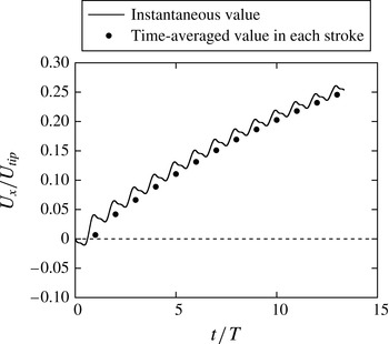
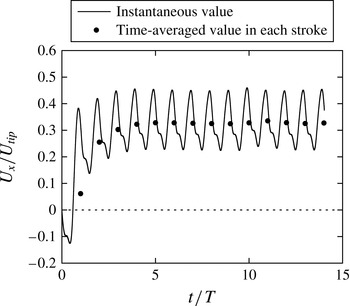
of the wing–body model for the condition of a fruit fly. Figure 14 shows
 $U_{x}$
and its averaged value in each stroke. Looking at the increasing rate of the averaged value, it cannot be expected that the forward speed of the wing–body model will reach the forward flight speed of a fruit fly, i.e.
 $U_{x}/U_{tip}=0.64$
(Shyy et al.
Reference Shyy, Lian, Tang, Viieru and Liu2008). This means that the thrust force generated by the wing–body model is smaller than that of a fruit fly. Therefore, the present wing–body model is not enough to generate a real thrust force. One might consider that the phase shift
 ${\it\gamma}$
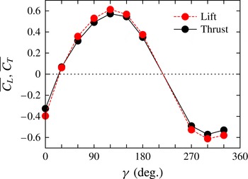
(see (2.5)) has a significant effect on the aerodynamic forces in the same way as the hovering fruit fly’s wing investigated by Dickinson et al. (Reference Dickinson, Lehman and Sane1999). Actually, the aerodynamic forces dramatically change as
 ${\it\gamma}$
changes also in the butterfly-like flapping wing–body model (see appendix D). However, the value used here,
 ${\it\gamma}=90^{\circ }$
, gives an almost maximal thrust force. Therefore, it is expected that even an optimal phase shift cannot give a comparable thrust force with a real insect. An actual insect may rely on the wing structure and the wing flexibility for generating a higher thrust force.
Time variations of the forward velocity
 $U_{x}$
of the wing–body model for the condition of a fruit fly (
 $L=3~\text{mm}$
,
 $\mathit{Re}=620$
,
 $N_{M}=61$
). The instantaneous value of
 $U_{x}$
and the time-averaged value of
 $U_{x}$
in each stroke are described.

5.2.2. Case for
$L=18.1~\text{mm}$

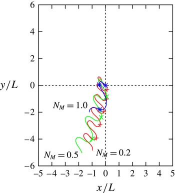
Figure 15 shows the trajectories of the COM of the wing–body model with
 $N_{M}=0.2$
, 0.5 and 1.0 (in the dimensional mass,
 $M=1.43$
, 3.57 and 7.15 mg, respectively) for
 $\mathit{Re}=500$
in the case of
 $L=18.1~\text{mm}$
. Note that
 $N_{M}=0.5$
is equal to the non-dimensional expected supportable mass
 $N_{Mexp}$
for
 $\mathit{Re}=500$
. It can be seen from figure 15 that the wing–body model with
 $N_{M}=N_{Mexp}$
goes downward. Moreover, the model even with
 $N_{M}=0.2<N_{Mexp}$
also goes downward. These results are quite different from those in the case of
 $L=3.0~\text{mm}$
shown in figure 12. This is because the non-dimensional masses in this case are much smaller than those in the previous case. That is, if the body is very light compared with the fluid, the body easily goes up and down by the force generated by the wings during each stroke; the body goes upward and downward during the downstroke and the upstroke of the wings, respectively. Thus, the velocity of the wing tips relative to the coordinate system fixed to the space decreases. Consequently, the wings cannot generate enough time-averaged lift during the stroke. It should be noted that the dimensional mass for
 $L=18.1~\text{mm}$
is actually much larger than that for
 $L=3.0~\text{mm}$
, since the non-dimensional mass is the mass of the body relative to the mass of the fluid in the volume
 $L^{3}$
. Therefore, this result suggests that it is difficult to support not a small dimensional mass but a small non-dimensional mass.
Trajectories of the COM of the wing–body model with
 $N_{M}=0.2$
, 0.5 and 1.0 for
 $\mathit{Re}=500$
. The initial position of the COM (the centre of the domain) is denoted by
 $(x/L,y/L)=(0,0)$
. The symbols on the trajectories indicate the position of the COM when the wings are at the top dead point.

In the same way as the previous case of
 $L=3.0~\text{mm}$
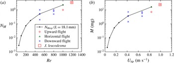
, we calculate free flights for various Reynolds numbers and non-dimensional masses. The results are shown in figure 16(a) with the non-dimensional parameters and in figure 16(b) with the dimensional parameters, respectively. In the figures, the non-dimensional expected supportable masses are also plotted. Unlike the case for
 $L=3.0~\text{mm}$
, the wing–body model with
 $N_{M}\leqslant N_{Mexp}$
goes downward for
 $\mathit{Re}<1000$
. However, for
 $\mathit{Re}\geqslant 1000$
, the model with
 $N_{M}\leqslant N_{Mexp}$
can go upward or keep altitude. In particular, the model with the same condition as a J. leucodesma can go upward against gravity. This result supports the same conclusion as the case of
 $L=3.0~\text{mm}$
, that is, even a simple wing–body model can generate an enough lift force to support real insects’ weight for
 $L=18.1~\text{mm}$
.
The map of (a)
 $\mathit{Re}{-}N_{M}$
and (b)
 $U_{tip}{-}M$
containing the expected supportable mass and points describing upward flight, almost horizontal flight or downward flight for
 $L=18.1~\text{mm}$
. The condition of a J. leucodesma is also described.

Figure 17 shows the forward velocity
 $U_{x}$
and its time-averaged value in each stroke for the parameters of a J. leucodesma. We can see from figure 17 that
 $U_{x}$
largely oscillates in one stroke and the averaged value of
 $U_{x}$
reaches the terminal forward speed at
 $t/T=14$
, since the non-dimensional mass is small as mentioned above. The terminal forward speed of the wing–body model
 $U_{x}/U_{tip}=0.32$
is smaller than the forward flight speed of a J. leucodesma
 $U_{x}/U_{tip}=0.77$
(Dudley Reference Dudley1990). This result is similar to the case of a fruit fly as shown in § 5.2.1. The Strouhal number defined by using the stroke amplitude and the terminal forward speed is
 $\mathit{St}=4{\it\theta}_{m}F_{req}L/U_{x}=U_{tip}/U_{x}=3.13$
.
Time variations of the forward velocity
 $U_{x}$
of the wing–body model for the condition of a J. leucodesma (
 $L=18.1~\text{mm}$
,
 $\mathit{Re}=1190$
,
 $N_{M}=3.36$
). The instantaneous value of
 $U_{x}$
and the time-averaged value of
 $U_{x}$
in each stroke are described.

5.3. Free flight (with rotation) simulation
Third, in order to investigate the body rotation, we simulate free flights of the wing–body model when the body can move translationally and rotationally. In this simulation, we set
 ${\it\alpha}_{m}=90^{\circ }$
,
 $L=3.0~\text{mm}$
,
 $N_{M}=38$
and
 $\mathit{Re}=300$
. Note that
 $N_{M}=38$
is equal to the non-dimensional expected supportable mass for
 $\mathit{Re}=300$
, that is, the wing–body model can go upward against gravity as shown in figure 13(a). As shown in figure 16(a), the upward flight with
 $L=18.1~\text{mm}$
can be achieved only for
 $\mathit{Re}\geqslant 1000$
. However, computations of three-dimensional moving boundary flows for
 $\mathit{Re}\geqslant 1000$
are quite expensive. On the other hand, the condition of
 $\mathit{Re}=300$
and
 $L=3.0~\text{mm}$
is much easier to be calculated and is a typical condition resulting in the upward flight. So, we use
 $L=3.0~\text{mm}$
instead of
 $L=18.1~\text{mm}$
in the following.
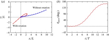
Figure 18 shows the trajectory of the COM and the time variation of the pitching angle of the body
 ${\it\theta}_{pitch}$
. The pitching angle
 ${\it\theta}_{pitch}$
is calculated by
 $$\begin{eqnarray}{\it\theta}_{pitch}=\arctan \left(\frac{2(q_{1}q_{3}+q_{2}q_{4})}{q_{0}^{2}+q_{1}^{2}-q_{2}^{2}-q_{3}^{2}}\right).\end{eqnarray}$$
It should be noted that also in this result the flow fields are symmetrical with respect to the longitudinal plane,
 $\boldsymbol{U}_{c}=(U_{x},U_{y},0)^{\text{T}}$
, and
 $~^{b}{\it\bf\Omega}_{c}=(0,{\it\omega}_{2},0)^{\text{T}}$
, while no assumption about the flow field and the body motion is used for
 $\mathit{Re}\leqslant 500$
(see § 4). It can be seen from figure 18(a,b) that the pitching angle
 ${\it\theta}_{pitch}$
increases gradually, and eventually the wing–body model turns over. This means that the present wing–body model obtains a positive mean pitching moment, while the mean pitching moment almost vanishes when the body of the wing–body model is fixed. This is because the mean centre of pressure moves backward due to the forward motion of the wing–body model. It has been reported also in Yokoyama et al. (Reference Yokoyama, Senda, Iima and Hirai2013) that the periodic flapping flights of a butterfly are longitudinally unstable and the control of the pitching angle is essential.
(a) Trajectories of the COM of the body and (b) time variation of the pitching angle of the body. In (a), the initial position of the COM (the centre of the domain) is denoted by
 $(x/L,y/L)=(0,0)$
, and the symbols on the trajectories indicate the position of the COM when the wings are at the top dead point.

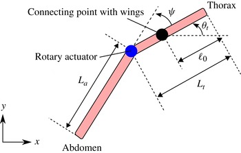
The body composed of the thorax and the abdomen for controlling the pitching angle of the wing–body model.

5.4. Computation for controlling the rotational motion
Finally, we discuss a way to control the pitching angle of the body. It is known that the body of an actual butterfly is composed of the thorax and the abdomen, and the pitching angle of the body is controlled by flexing at the joint between the thorax and the abdomen (Dudley Reference Dudley2002). In this study, we attempt to control the pitching angle of the body by using a modified wing–body model whose body is composed of the thorax and the abdomen like an actual butterfly. Here, we assume that the body moves only in the
 $x$
and
 $y$
directions and rotates only in the pitching motion for simplicity.
5.4.1. Computational model for controlling the pitching motion
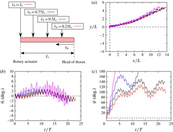
Let the body be composed of two straight infinitely thin rods (see figure 19): the thorax with length
 $L_{t}$
and the abdomen with length
 $L_{a}$
. The total length of the body is
 $L_{b}=L_{t}+L_{a}$
. Let the mass of the thorax be
 $M_{t}$
and that of the abdomen be
 $M_{a}$
. The total mass of the body is
 $M=M_{t}+M_{a}$
. The connecting point between the thorax and the wings is located at the distance of
 $\ell _{0}$
from the head of the thorax. In this study, we set
 $L_{b}=0.75L$
,
 $L_{t}:L_{a}=3:7$
,
 $M_{t}:M_{a}=44:51$
and
 $\ell _{0}=0.77L_{t}$
, which are the same as a J. leucodesma (Dudley Reference Dudley1990). We assume that the thorax and the abdomen are connected by a rotary actuator with no mass and no rotation friction. The shape and the motion of the wings of the modified wing–body model are the same as the original wing–body model. We attempt to control the pitching angle of the thorax
 ${\it\theta}_{t}$
by the input torque
 $T^{cont}$
produced by the rotary actuator. The equations of motion of the thorax and the abdomen are shown in appendix E.
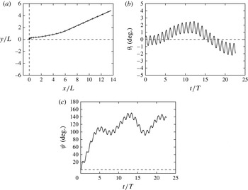
(a) Trajectory of the COM of the thorax, (b) time variation of the pitching angle of the thorax and (c) time variation of the relative angle of the abdomen to the thorax when the pitching angle of the thorax is controlled by flexing at the joint between the thorax and the abdomen. In (a), the initial position of the COM (the centre of the domain) is denoted by
 $(x/L,y/L)=(0,0)$
, and the symbols on the trajectories indicate the position of the COM when the wings are at top dead point.

In this study, we consider the proportional–integral–derivative (PID) control, i.e. the input torque
 $T^{cont}$
is determined by
 $$\begin{eqnarray}T^{cont}(t)=K_{p}({\it\theta}_{0}(t)-{\it\theta}_{t}(t))+K_{i}\int _{0}^{t}({\it\theta}_{0}(t^{\prime })-{\it\theta}_{t}(t^{\prime }))\text{d}t^{\prime }+K_{d}(\dot{{\it\theta}}_{0}(t)-\dot{{\it\theta}}_{t}(t)),\end{eqnarray}$$
where
 ${\it\theta}_{0}$
is the desired pitching angle of the thorax,
 $K_{p}$
is the proportional gain,
 $K_{i}$
is the integral gain and
 $K_{d}$
is the derivative gain. In order to suppress the increase in the pitching angle
 ${\it\theta}_{t}$
, we set
 ${\it\theta}_{0}(t)=0^{\circ }$
. It should be noted that in this control there are three tuning parameters, i.e.
 $K_{p}$
,
 $K_{i}$
and
 $K_{d}$
.
5.4.2. Calculation example
We calculate the motion of the wing–body model under the above control for the same condition as § 5.3, i.e.
 ${\it\alpha}_{m}=90^{\circ }$
,
 $L=3.0~\text{mm}$
,
 $N_{M}=38$
and
 $\mathit{Re}=300$
. In this simulation, we set
 $K_{p}=-M_{a}L_{a}^{2}F_{req}^{2}\times 0.698$
,
 $K_{i}=-M_{a}L_{a}^{2}F_{req}^{3}\times 0.698$
and
 $K_{d}=-M_{a}L_{a}^{2}F_{req}\times 9.65$
as an example. Figure 20 shows the trajectory of the COM of the thorax, the time variation of the pitching angle
 ${\it\theta}_{t}$
and the time variation of the relative angle
 ${\it\psi}$
. It can be seen from figure 20(a) that the wing–body model can go upward. In figure 20(b), the pitching angle is controlled in the ranges of
 $|{\it\theta}_{t}|<5^{\circ }$
beyond 20 strokes. In addition, we can see form figure 20(c) that the relative angle
 ${\it\psi}$
of the abdomen to the thorax increases at first, and then oscillates around
 $120^{\circ }$
. This result means that the pitching angle of the thorax can be controlled by flexing at the joint between the thorax and the abdomen like an actual butterfly. However, the range of the relative angle is very unrealistic.
Since the position of the centre of pressure is very important in the stability of aircrafts, one might consider that the position of the connecting point between the thorax and the wings, which is determined by
 $\ell _{0}$
in this model, has a significant effect on the behaviour of the relative angle
 ${\it\psi}$
. Figure 21 shows the results for
 $\ell _{0}=L_{t}$
,
 $0.77L_{t}$
,
 $0.5L_{t}$
and
 $0.23L_{t}$
. It is noted that the results for
 $\ell _{0}=0.77L_{t}$
is the same as figure 20. It can be seen from figure 21(a,b) that while in all cases the wing–body model can go upward, the oscillation of the pitching angle
 ${\it\theta}_{t}$
becomes more suppressed as
 $\ell _{0}$
increases, that is, the connecting point between the thorax and the wings gets away from the head of the thorax. Also, we can see from figure 21(c) that the range of the relative angle
 ${\it\psi}$
becomes more limited as
 $\ell _{0}$
increases. Therefore, the stability of the wing–body model is improved as
 $\ell _{0}$
increases. However, even for the most stable case of
 $\ell _{0}=L_{t}$
, the relative angle varies in an unrealistic range.
The effect of
 $\ell _{0}$
on (a) trajectory of the COM of the thorax, (b) time variation of the pitching angle of the thorax and (c) time variation of the relative angle of the abdomen to the thorax. In (a), the initial position of the COM (the centre of the domain) is denoted by
 $(x/L,y/L)=(0,0)$
, and the symbols on the trajectories indicate the position of the COM when the wings are at the top dead point.

It should be noted that the conditions in this simulation (
 $L=3.0~\text{mm}$
,
 $N_{M}=38$
and
 $\mathit{Re}=300$
) are much different from those of an actual butterfly. The difference of the conditions may be a cause that the relative angle varies in an unrealistic range. The calculation for the condition of an actual butterfly and the optimization control remain for future work.
In the view point of the actual insect flight mechanisms, the present wing–body model is not sufficient to explain the mechanisms completely, since the present model is highly idealized and neglects many important factors, e.g. the wing structure, the wing flexibility, the mass of the wings and so on. Therefore, the results obtained by the present model just suggest a possibility that flexing the body may affect the stability of flapping flight by insects. From the view point of practical implementations for MAVs, the frequency of the pitching angle is so high that the control mechanism cannot be applied directly to practical implementations. Therefore, an intermittent control with a practical interval should be considered for practical implementations.
6. Conclusions
We have investigated lift and thrust generation by a simple butterfly-like flapping wing–body model. The wing–body model is composed of two rectangular wings and a rod-shaped body, and the wings and the body are rigid and infinitely thin. The wing–body model flaps downward for generating the lift force and backward for generating the thrust force like a butterfly. In this study, the following four kinds of simulations were implemented by using the IB-LBM: (i) the computation of aerodynamic forces; (ii) free flight (without rotation) simulations; (iii) free flight (with rotation) simulations; and (iv) the computation for controlling the rotational motion.
First, we calculated flows around the wing–body model and the aerodynamic forces for various Reynolds numbers of
 $50\leqslant \mathit{Re}\leqslant 1000$
, when the body of the wing–body model is fixed. As results, we found that the time-averaged lift coefficient
 $\overline{C_{L}}$
and the time-averaged thrust coefficient
 $\overline{C_{T}}$
increase as the Reynolds number and the maximum angle of attack increase. However, the rate of increase both in
 $\overline{C_{L}}$
and
 $\overline{C_{T}}$
against the Reynolds number becomes smaller as the Reynolds number increases. In addition, it was found that the time-averaged power coefficient decreases and therefore the efficiency increases as the Reynolds number and the maximum angle of attack increase. Moreover, we estimated the expected supportable mass for each Reynolds number by using
 $\overline{C_{L}}$
, and found that the mass of a fruit fly (D. melanogaster) and a small butterfly (J. leucodesma) can be supported against gravity.
Second, we simulated free flights when the body of the wing–body model can only move translationally. It was found that the expected supportable mass can be supported even in the free flight except when the mass of the body relative to the mass of the fluid is too small. In addition, it was found that the wing–body model with the mass of actual insects (a fruit fly and a small butterfly) can go upward against gravity at the actual Reynolds number, but cannot achieve the forward speed of actual insects.
Finally, we simulated free flights when the body of the wing–body model can move translationally and rotationally, and found that the body has a large pitching motion and consequently gets off-balance. Then, we showed that the pitching motion of the body can be controlled by flexing at the joint between the thorax and the abdomen like an actual butterfly.
It is highlighted that even a simple wing–body model with rigid wings can generate a realistic lift force and can stabilize its attitude by a simple control method. These results encourage that an artificial flapping MAV with simple rigid wings and simple mechanisms can be achieved. It should be noted that many important factors (e.g. the wing structure, the wing flexibility, the mass of the wings and so on) are not considered in the present wing–body model, and may lead to different conclusions. Therefore, the present model is not sufficient to explain the actual insect flight mechanisms completely. For example, Shyy et al. (Reference Shyy, Aono, Chimakurthi, Trizila, Kang, Cesnik and Liu2010) suggests that the wing flexibility in actual insects’ wings is expected to considerably affect the lift and thrust generations and the flight stability. So, the present results based on rigid wings may change considerably if the wing flexibility is considered. The effect of the flexibility of the wing remains in future work.
Acknowledgements
This research used computational resources of the HPCI system provided by ACCMS (Kyoto University) through the HPCI System Research Project (Project ID: hp120112). K. Suzuki acknowledges the financial support of the JSPS Institutional Program for Young Researcher Overseas Visits and Grant-in-Aid for JSPS Fellows (No. 25
 $\cdot$
1557). The authors would like to thank Dr A. Medina for help with the simulation in § B.2 and for providing his data computed by using the IB-FVM.
Appendix A. Formulation of the kinematic equations
In this section, we look at the kinematics of the body described by the quaternion. The orthogonal matrix represented by a unit quaternion
 $\unicode[STIX]{x1D64E}(\boldsymbol{Q})$
is given by
 $$\begin{eqnarray}\unicode[STIX]{x1D64E}(\boldsymbol{Q})=\left[\begin{array}{@{}ccc@{}}q_{0}^{2}-q_{2}^{2}-q_{3}^{2}+q_{1}^{2} & 2(q_{1}q_{2}-q_{0}q_{3}) & 2(q_{1}q_{3}+q_{0}q_{2})\\ 2(q_{1}q_{2}+q_{0}q_{3}) & q_{0}^{2}-q_{3}^{2}-q_{1}^{2}+q_{2}^{2} & 2(q_{2}q_{3}-q_{0}q_{1})\\ 2(q_{1}q_{3}-q_{0}q_{2}) & 2(q_{2}q_{3}+q_{0}q_{1}) & q_{0}^{2}-q_{1}^{2}-q_{2}^{2}+q_{3}^{2}\end{array}\right],\end{eqnarray}$$
where
 $$\begin{eqnarray}q_{0}^{2}+q_{1}^{2}+q_{2}^{2}+q_{3}^{2}=1.\end{eqnarray}$$
The initial value of the quaternion is set to be
 $\boldsymbol{Q}(0)=((1/\sqrt{2}),(1/\sqrt{2}),0,0)^{\text{T}}$
so that
 $\unicode[STIX]{x1D64E}(\boldsymbol{Q}(0))=\unicode[STIX]{x1D64E}_{1}(90^{\circ })$
for setting the initial direction of the axes of
 ${\it\Sigma}_{b}$
. We refer the reader to Shuster (Reference Shuster1993) and Goldstein, Poole & Safko (Reference Goldstein, Poole and Safko2002) for more details of the quaternion.
Let
 $\boldsymbol{U}_{c}(t)$
be the velocity of
 $\boldsymbol{X}_{c}(t)$
and
 $~^{b}{\it\bf\Omega}_{c}(t)$
be the angular velocity of the body. The kinematic equations of the body are as follows:
 $$\begin{eqnarray}\displaystyle & \displaystyle \frac{\text{d}\boldsymbol{X}_{c}}{\text{d}t}=\boldsymbol{U}_{c}(t), & \displaystyle\end{eqnarray}$$
 $$\begin{eqnarray}\displaystyle & \displaystyle \frac{\text{d}\boldsymbol{Q}}{\text{d}t}=\unicode[STIX]{x1D63C}(t)\boldsymbol{Q}(t), & \displaystyle\end{eqnarray}$$
 $\unicode[STIX]{x1D63C}(t)$
is a
 $4\times 4$
matrix which is determined by
 $~^{b}{\it\bf\Omega}_{c}=({\it\omega}_{1},{\it\omega}_{2},{\it\omega}_{3})^{\text{T}}$
as follows:
 $$\begin{eqnarray}\unicode[STIX]{x1D63C}={\displaystyle \frac{1}{2}}\left[\begin{array}{@{}cccc@{}}0 & -{\it\omega}_{1} & -{\it\omega}_{2} & -{\it\omega}_{3}\\ {\it\omega}_{1} & 0 & {\it\omega}_{3} & -{\it\omega}_{2}\\ {\it\omega}_{2} & -{\it\omega}_{3} & 0 & {\it\omega}_{1}\\ {\it\omega}_{3} & {\it\omega}_{2} & -{\it\omega}_{1} & 0\end{array}\right].\end{eqnarray}$$
Appendix B. Accuracy of the numerical method
In order to examine the accuracy of the present numerical method, we have calculated typical flows around a flat plate, around a flapping wing with a finite thickness and around the fruit fly’s wing which has been investigated by Dickinson et al. (Reference Dickinson, Lehman and Sane1999).
B.1. Flow around a flat plate
In order to examine the accuracy of the present numerical method, we have calculated the flow around a rectangular flat plate by the IB-LBM. The flat plate is an infinitely thin rectangular plate as shown in figure 1(a) with
 $L=2c$
. The flat plate is set in a uniform flow whose speed is
 $U_{\infty }$
with an angle of attack
 ${\it\alpha}$
. The Reynolds number defined by
 $\mathit{Re}=U_{\infty }c/{\it\nu}$
is set to 100. Let the
 $x$
-axis be parallel to the uniform flow, the
 $y$
-axis be the upward direction and the
 $z$
-axis be the span direction of the flat plat. The computational domain is
 $[-4c,6c]\times [-5c,5c]\times [-5c,5c]$
, and the centre of the flat plate is located at the origin. Boundary conditions on all sides of the domain are set to the uniform flow
 $\boldsymbol{u}=(U_{\infty },0,0)$
except for the outlet boundary where a Neumann boundary condition, i.e.
 $\partial \boldsymbol{u}/\partial x=\mathbf{0}$
and
 $\partial p/\partial x=0$
is used. In the simulation by the IB-LBM, we use a multi-block grid (Inamuro Reference Inamuro2012) in order to save computation time. The multi-block grid is composed of a fine grid with
 ${\rm\Delta}x$
in
 $[-1.4c,5.8c]\times [2.4c,2.4c]\times [1.4c,1.4c]$
where
 $c=50{\rm\Delta}x$
and a coarse grid with
 $2{\rm\Delta}x$
in the other domain. We calculate the lift coefficient
 $C_{L}=2F_{y}/({\it\rho}_{f}U_{\infty }^{2}Lc)$
and the drag coefficient
 $C_{D}=2F_{x}/({\it\rho}_{f}U_{\infty }^{2}Lc)$
for various angles of attack of
 $0^{\circ }\leqslant {\it\alpha}\leqslant 90^{\circ }$
. Figure 22 shows
 $C_{L}$
and
 $C_{D}$
against
 ${\it\alpha}$
at
 $t/(c/U_{\infty })=13$
. The results by the present method agree well with the experimental and numerical results by Taira & Colonius (Reference Taira and Colonius2009).
Lift and drag coefficients for a rectangular plate with
 $L=2c$
in a uniform flow at
 $\mathit{Re}=100$
. The results by the present IB-LBM are compared with the experimental and numerical results by Taira & Colonius (Reference Taira and Colonius2009).

B.2. Flow around a flapping wing with a finite thickness
The second problem is a flow around a flapping wing with a finite thickness. The wing has a thin-cuboid shape with the tip length
 $c$
, the wing length
 $L$
and the thickness
 $w$
. In this simulation, we set
 $L=2c$
and
 $w=0.1c$
. The wing flaps and changes its angle of attack in fluid at rest.
Let the coordinate system fixed to the wing be
 ${\it\Sigma}_{w}$
, and the coordinate system fixed to the space be
 ${\it\Sigma}_{s}$
. We denote the axes and the unit vectors along the axes of
 ${\it\Sigma}_{w}$
and
 ${\it\Sigma}_{s}$
using the same notation as in §§ 2 and 3. The
 ${\it\eta}$
-axis lies on the centre plane between the front and back sides of the wing and is normal to the tip side. The
 ${\it\zeta}$
-axis lies on the centre plane between the front and back sides of the wing and is normal to the top side. The distance of the origin of
 ${\it\Sigma}_{w}$
from the top side is d and that from the root side is
 $r_{s}$
(see figure 23
a). In this simulation, we set
 $d=0.16c$
and
 $r_{s}=0.4c$
. The vector array
 $[\boldsymbol{e}_{{\it\xi}},\boldsymbol{e}_{{\it\eta}},\boldsymbol{e}_{{\it\zeta}}]$
is given by the successive orthogonal transformations of
 $[\boldsymbol{e}_{x},\boldsymbol{e}_{y},\boldsymbol{e}_{z}]$
as follows:
 $$\begin{eqnarray}[\boldsymbol{e}_{{\it\xi}},\boldsymbol{e}_{{\it\eta}},\boldsymbol{e}_{{\it\zeta}}]=[\boldsymbol{e}_{x},\boldsymbol{e}_{y},\boldsymbol{e}_{z}]\unicode[STIX]{x1D64E}_{3}({\it\phi}(t))\unicode[STIX]{x1D64E}_{2}({\it\beta}(t))\unicode[STIX]{x1D64E}_{1}(0),\end{eqnarray}$$
where
 ${\it\phi}(t)$
and
 ${\it\beta}(t)$
are the flapping angle and the rotational angle at time
 $t$
, respectively, given by
 $$\begin{eqnarray}\displaystyle & \displaystyle {\it\phi}(t)={\it\phi}_{m}\cos \left(\frac{2{\rm\pi}}{T}t\right), & \displaystyle\end{eqnarray}$$
 $$\begin{eqnarray}\displaystyle & \displaystyle {\it\beta}(t)=\frac{{\it\beta}_{m}}{\tanh C_{{\it\eta}}}\tanh \left(C_{{\it\eta}}\sin \left(\frac{2{\rm\pi}}{T}t\right)\right), & \displaystyle\end{eqnarray}$$
 ${\it\phi}_{m}$
is the maximum flapping angle,
 ${\it\beta}_{m}$
is the maximum rotational angle and
 $C_{{\it\eta}}$
is a rotational shape parameter. In this simulation, we set
 ${\it\phi}_{m}=80^{\circ }$
,
 ${\it\beta}_{m}=45^{\circ }$
and
 $C_{{\it\eta}}=3.3$
. The time variation of the rotational angle
 ${\it\beta}$
and the flapping angle
 ${\it\phi}$
are shown in figure 23(b). The Reynolds number defined by
 $\mathit{Re}=U_{tip}c/{\it\nu}$
where
 $U_{tip}=2{\rm\pi}{\it\phi}_{m}(r_{s}+L)/T$
is set to 100.
(a) The wing with a finite thickness and the coordinate system fixed to the wing (
 ${\it\xi}{-}{\it\eta}{-}{\it\zeta}$
) and (b) the time variations of the rotational angle
 ${\it\beta}$
and the flapping angle
 ${\it\phi}$
.

In the simulation by the IB-LBM, we use a computational domain with
 $[-5c,5c]\times [-3.9c,6.1c]\times [-5.3c,4.7c]$
. As for the boundary condition of the domain, a Neumann boundary condition, i.e.
 $(\boldsymbol{n}\boldsymbol{\cdot }\boldsymbol{{\rm\nabla}})\boldsymbol{u}=\mathbf{0}$
and
 $\boldsymbol{n}\boldsymbol{\cdot }\boldsymbol{{\rm\nabla}}p=0$
(
 $\boldsymbol{n}$
is the unit vector normal to the boundary) is used on all sides of the domain. It should be noted that in our preliminary calculations where the no-slip boundary condition is used on all sides of the domain the results for the Neumann boundary condition is almost coincident with those for the no-slip boundary condition. We use a multi-block grid (Inamuro Reference Inamuro2012) composed of a fine grid with
 ${\rm\Delta}x$
in
 $[-2.6c,2.6c]\times [-0.5c,2.7c]\times [-1.05c,0.45c]$
and a coarse grid with
 $2{\rm\Delta}x$
in the other domain. In this simulation, we set
 $c=50{\rm\Delta}x$
and
 $T=35\,092{\rm\Delta}t$
. The rigid-body approximation is used for the internal mass effect (see Suzuki & Inamuro Reference Suzuki and Inamuro2011).
We calculate the lift coefficient
 $C_{L}=2F_{z}/({\it\rho}_{f}U_{tip}^{2}Lc)$
and the drag coefficient
 $C_{D}=2F_{x}/({\it\rho}_{f}U_{tip}^{2}Lc)$
. Figure 24 shows the time variations of
 $C_{L}$
and
 $C_{D}$
in
 $3\leqslant t/T\leqslant 4$
. The results by the present method agree well with the numerical results computed by Medina (Reference Medina2013) using the immersed boundary–finite volume method (IB-FVM) proposed by Kim, Kim & Choi (Reference Kim, Kim and Choi2001).
Time variations of lift coefficient
 $C_{L}$
and drag coefficient
 $C_{D}$
for a flapping wing at
 $\mathit{Re}=100$
. The results by the present IB-LBM are compared with the numerical results by IB-FVM.

The planform of the fruit fly’s wing and the coordinate system fixed to the wing (
 ${\it\xi}{-}{\it\eta}{-}{\it\zeta}$
).

B.3. Flow around the fruit fly’s wing
The third problem is a flow around the fruit fly’s wing which has been investigated by Dickinson et al. (Reference Dickinson, Lehman and Sane1999). The planform of the fruit fly’s wing used here (see figure 25) is copied from that in Wu & Sun (Reference Wu and Sun2004), which is the same as that of the robotic fruit fly wing used by Dickinson et al. (Reference Dickinson, Lehman and Sane1999). The wing length
 $L$
is 250 mm, and the airfoil of the wing is flat with thickness of 3.2 mm and two half-circle edges. The wing flaps and changes its angle of attack in a
 $1~\text{m}\times 1~\text{m}\times 2~\text{m}$
tank of mineral oil with the density of
 $880~\text{kg}~\text{m}^{-3}$
and the kinematic viscosity of
 $1.15\times 10^{-4}~\text{m}^{2}~\text{s}^{-1}$
at rest. In this study, we simulate the experiments shown in figure 3A–C of Dickinson et al. (Reference Dickinson, Lehman and Sane1999). In these experiments, the stroke amplitude is
 ${\it\Phi}=160^{\circ }$
, the frequency
 $F_{req}=0.145~\text{Hz}$
and the angle of attack at midstroke is
 ${\it\alpha}_{m}=40^{\circ }$
.
Let the coordinate system fixed to the wing be
 ${\it\Sigma}_{w}$
, and the coordinate system fixed to the space be
 ${\it\Sigma}_{s}$
. We denote the axes and the unit vectors along the axes of
 ${\it\Sigma}_{w}$
and
 ${\it\Sigma}_{s}$
by the same notation as § B.2. The
 ${\it\eta}$
and
 ${\it\zeta}$
axes are defined as shown in figure 25, and the
 ${\it\xi}$
-axis is defined so that
 ${\it\Sigma}_{w}$
can be a right-handed system. The distances of the
 ${\it\zeta}$
-axis from the wing tip and the wing root are
 $L$
and
 $r_{s}$
, respectively. We define the chord length at
 ${\it\eta}=0.5L$
as the mean chord length
 $c_{m}$
. The distance of the
 ${\it\eta}$
-axis from the leading edge at
 ${\it\eta}=0.5L$
is d. In this simulation, we set
 $r_{s}=0.145L$
and
 $d=0.25c_{m}$
.
The vector array
 $[\boldsymbol{e}_{{\it\xi}},~\boldsymbol{e}_{{\it\eta}},~\boldsymbol{e}_{{\it\zeta}}]$
is given in the same way as (B 1), but the flapping angle
 ${\it\phi}$
and the rotational angle
 ${\it\beta}$
are different from (B 2) and (B 3). In this study, we use the following mathematical formulations of
 ${\it\phi}$
and
 ${\it\beta}$
which have been used in many numerical studies (e.g. Sun & Tang Reference Sun and Tang2002; Gilmanov & Sotiropoulos Reference Gilmanov and Sotiropoulos2005; Bai et al.
Reference Bai, Cui, Zhou and Chen2007):
 $$\begin{eqnarray}\displaystyle & \displaystyle {\it\phi}(t)=\left\{\begin{array}{@{}l@{}}\displaystyle {\it\phi}_{0}-{\it\omega}_{{\it\phi}}\frac{{\rm\Delta}{\it\tau}_{t}}{{\rm\pi}}\left[1-\cos \left(\frac{{\rm\pi}t}{{\rm\Delta}{\it\tau}_{t}}\right)\right],\quad \displaystyle \left(0\leqslant t<\frac{{\rm\Delta}{\it\tau}_{t}}{2}\right),\quad \\ \displaystyle {\it\phi}_{0}+{\it\omega}_{{\it\phi}}\left[\left(\frac{1}{2}-\frac{1}{{\rm\pi}}\right){\rm\Delta}{\it\tau}_{t}-t\right],\quad \displaystyle \left(\frac{{\rm\Delta}{\it\tau}_{t}}{2}\leqslant t<\frac{T}{2}-\frac{{\rm\Delta}{\it\tau}_{t}}{2}\right),\quad \\ \displaystyle {\it\phi}_{0}+{\it\omega}_{{\it\phi}}\left[\left(1-\frac{1}{{\rm\pi}}\right){\rm\Delta}{\it\tau}_{t}-\frac{T}{2}-\frac{{\rm\Delta}{\it\tau}_{t}}{{\rm\pi}}\cos \left(\frac{{\rm\pi}(t-T/2)}{{\rm\Delta}{\it\tau}_{t}}\right)\right],\quad \left(\frac{T}{2}-\frac{{\rm\Delta}{\it\tau}_{t}}{2}\leqslant t<\frac{T}{2}+\frac{{\rm\Delta}{\it\tau}_{t}}{2}\right),\quad \\ \displaystyle {\it\phi}_{0}+{\it\omega}_{{\it\phi}}\left[\left(\frac{1}{2}-\frac{1}{{\rm\pi}}\right){\rm\Delta}{\it\tau}_{t}-T+t\right],\quad \displaystyle \left(\frac{T}{2}+\frac{{\rm\Delta}{\it\tau}_{t}}{2}\leqslant t<T-\frac{{\rm\Delta}{\it\tau}_{t}}{2}\right),\quad \\ \displaystyle {\it\phi}_{0}-{\it\omega}_{{\it\phi}}\frac{{\rm\Delta}{\it\tau}_{t}}{{\rm\pi}}\left[1-\cos \left(\frac{{\rm\pi}(t-T)}{{\rm\Delta}{\it\tau}_{t}}\right)\right],\quad \displaystyle \left(T-\frac{{\rm\Delta}{\it\tau}_{t}}{2}\leqslant t<T\right),\quad \end{array}\right. & \displaystyle\end{eqnarray}$$
 $$\begin{eqnarray}\displaystyle & \displaystyle {\it\beta}(t)=\left\{\begin{array}{@{}l@{}}\displaystyle {\it\beta}_{0}+\frac{{\it\omega}_{{\it\beta}}}{2}\left[t+\frac{{\rm\Delta}{\it\tau}_{r}}{2{\rm\pi}}\sin \left(\frac{2{\rm\pi}t}{{\rm\Delta}{\it\tau}_{r}}\right)\right],\quad \displaystyle \left(0\leqslant t<\frac{{\rm\Delta}{\it\tau}_{r}}{2}\right),\quad \\ \displaystyle {\it\beta}_{0}+\frac{{\it\omega}_{{\it\beta}}}{2}\frac{{\rm\Delta}{\it\tau}_{r}}{2},\quad \displaystyle \left(\frac{{\rm\Delta}{\it\tau}_{r}}{2}\leqslant t<\frac{T}{2}-\frac{{\rm\Delta}{\it\tau}_{r}}{2}\right),\quad \\ \displaystyle {\it\beta}_{0}-\frac{{\it\omega}_{{\it\beta}}}{2}\left[t-\frac{T}{2}+\frac{{\rm\Delta}{\it\tau}_{r}}{2{\rm\pi}}\sin \left(\frac{2{\rm\pi}(t-T/2)}{{\rm\Delta}{\it\tau}_{r}}\right)\right],\quad \left(\frac{T}{2}-\frac{{\rm\Delta}{\it\tau}_{r}}{2}\leqslant t<\frac{T}{2}+\frac{{\rm\Delta}{\it\tau}_{r}}{2}\right),\quad \\ \displaystyle {\it\beta}_{0}-\frac{{\it\omega}_{{\it\beta}}}{2}\frac{{\rm\Delta}{\it\tau}_{r}}{2},\quad \displaystyle \left(\frac{T}{2}+\frac{{\rm\Delta}{\it\tau}_{r}}{2}\leqslant t<T-\frac{{\rm\Delta}{\it\tau}_{r}}{2}\right),\quad \\ \displaystyle {\it\beta}_{0}+\frac{{\it\omega}_{{\it\beta}}}{2}\left[t-T+\frac{{\rm\Delta}{\it\tau}_{r}}{2{\rm\pi}}\sin \left(\frac{2{\rm\pi}(t-T)}{{\rm\Delta}{\it\tau}_{r}}\right)\right],\quad \displaystyle \left(T-\frac{{\rm\Delta}{\it\tau}_{r}}{2}\leqslant t<T\right),\quad \end{array}\right. & \displaystyle\end{eqnarray}$$
 ${\it\phi}_{0}$
,
 ${\it\omega}_{{\it\phi}}$
and
 ${\rm\Delta}{\it\tau}_{t}$
are the initial flapping angle, the maximum flapping angular velocity and the duration of the wing acceleration/deceleration, respectively, and
 ${\it\beta}_{0}$
,
 ${\it\omega}_{{\it\beta}}$
and
 ${\rm\Delta}{\it\tau}_{r}$
are the initial rotational angle, the maximum rotational angular velocity and the duration of the wing rotation. The above mathematical formulations are periodic and differentiable functions with the common period
 $T=1/F_{req}$
. It should be noted that the rotational angle
 ${\it\beta}(t)$
given in (B 5) is for the ‘symmetrical’ in figure 3B of Dickinson et al. (Reference Dickinson, Lehman and Sane1999). The ‘advanced’ and ‘delayed’ in figure 3A and C of Dickinson et al. (Reference Dickinson, Lehman and Sane1999) are given by using
 ${\it\beta}(t+{\it\tau}_{r0})$
and
 ${\it\beta}(t-{\it\tau}_{r0})$
instead of
 ${\it\beta}(t)$
, respectively, where
 ${\it\tau}_{r0}$
represents the timing of the rotation and is set to be
 $0.08T$
.
In the above formulation,
 ${\it\phi}$
changes in the range of
 ${\it\phi}_{0}-{\it\omega}_{{\it\phi}}[T/2-(1-{\rm\pi}/2){\rm\Delta}{\it\tau}_{t}]$
to
 ${\it\phi}_{0}$
, and
 ${\it\beta}$
changes in the range of
 ${\it\beta}_{0}-{\it\omega}_{{\it\beta}}{\rm\Delta}{\it\tau}_{r}/4$
to
 ${\it\beta}_{0}+{\it\omega}_{{\it\beta}}{\rm\Delta}{\it\tau}_{r}/4$
. Therefore, considering the stroke amplitude
 ${\it\Phi}$
and the angle of attack at midstroke
 ${\it\alpha}_{m}$
, we can obtain the following equations:
 $$\begin{eqnarray}\displaystyle & \displaystyle {\it\phi}_{0}=\frac{{\it\Phi}}{2}, & \displaystyle\end{eqnarray}$$
 $$\begin{eqnarray}\displaystyle & \displaystyle {\it\omega}_{{\it\phi}}\left[\frac{T}{2}-\left(1-\frac{{\rm\pi}}{2}\right){\rm\Delta}{\it\tau}_{t}\right]={\it\Phi}, & \displaystyle\end{eqnarray}$$
 $$\begin{eqnarray}\displaystyle & \displaystyle {\it\beta}_{0}=0, & \displaystyle\end{eqnarray}$$
 $$\begin{eqnarray}\displaystyle & \displaystyle \frac{{\it\omega}_{{\it\beta}}{\rm\Delta}{\it\tau}_{r}}{4}=\frac{{\rm\pi}}{2}-{\it\alpha}_{m}. & \displaystyle\end{eqnarray}$$
 ${\it\phi}_{0}$
,
 ${\it\omega}_{{\it\phi}}$
,
 ${\it\beta}_{0}$
and
 ${\it\omega}_{{\it\beta}}$
) are determined when
 ${\rm\Delta}{\it\tau}_{t}$
and
 ${\rm\Delta}{\it\tau}_{r}$
are given. In this study, we use the same parameters as Bai et al. (Reference Bai, Cui, Zhou and Chen2007), that is,
 ${\rm\Delta}{\it\tau}_{t}=0.1T$
and
 ${\rm\Delta}{\it\tau}_{r}=0.32T$
. The Reynolds number based on the mean chord length
 $c_{m}$
is
 $\mathit{Re}=2{\it\Phi}F_{req}Lc_{m}/{\it\nu}=110$
.
In the simulation by the IB-LBM, we use a computational domain with
 $[-2L,2L]\times [-2L,2L]\times [0,8L]$
, and the origin of
 ${\it\Sigma}_{w}$
is set at
 $(0,0.28L,6.4L)$
. As for the boundary condition of the domain, a no-slip boundary condition is used on all sides of the domain. In the experiments by Dickinson et al. (Reference Dickinson, Lehman and Sane1999), a liquid free surface exists at the top of the domain. In spite of this, we use the no-slip condition at the top of the domain instead of the free surface condition. This is because it is difficult to achieve the free surface condition, and the influence of the mismatch of the boundary conditions on the top of the domain is considered to be small. We use a multi-block grid (Inamuro Reference Inamuro2012) composed of a fine grid with
 ${\rm\Delta}x$
in
 $[-1.5L,1.5L]\times [-1.5L,1.5L]\times [5.6L,7.2L]$
and a coarse grid with
 $2{\rm\Delta}x$
in the other domain. In this simulation, we set
 $L=90{\rm\Delta}x$
and
 $T=15\,000{\rm\Delta}t$
. The rigid-body approximation is used for the internal mass effect (see Suzuki & Inamuro Reference Suzuki and Inamuro2011).
We calculate the lift force
 $F_{z}$
for the three modes: advanced, symmetrical and delayed. The simulations are conducted until
 $t=6T$
. The temporal variation of the lift force during each stroke is almost the same after
 $t=3T$
, and thus we present the results of fourth period in the following. Figure 26 shows the time variations of the lift force and the kinematics of the wing. The lift forces for the three modes obtained by the present method have reasonable agreements with the experiment by Dickinson et al. (Reference Dickinson, Lehman and Sane1999).
Comparison of the results between the IB-LBM and the experiment by Dickinson et al. (Reference Dickinson, Lehman and Sane1999). (a) Advanced, (b) symmetrical and (c) delayed. Upper figures show the lift force and lower figures show the translational velocity
 $U_{tip}=L\dot{{\it\phi}}$
(black) and the rotational velocity
 $\dot{{\it\alpha}}$
(red). Grey and white backgrounds mark downstroke and upstroke, respectively.

B.4. Summary and discussion on accuracy of the method
At the end of this appendix, we summarize the above three validations and discuss the accuracy of the method.
In the first validation, the flow around a stationary flat plate at
 $\mathit{Re}=100$
is simulated, and the lift and drag coefficients obtained by the present method agree well with the experimental and numerical results by Taira & Colonius (Reference Taira and Colonius2009). In the second validation, the flow around a flapping wing with a finite thickness at
 $\mathit{Re}=100$
is simulated, and the time variations of the lift and drag coefficients obtained by the present method agree well with the numerical results computed by Medina (Reference Medina2013) using the IB-FVM proposed by Kim et al. (Reference Kim, Kim and Choi2001). In the third validation, the flow around the fruit fly’s wing around
 $\mathit{Re}=100$
is simulated, and the lift forces obtained by the present method have reasonable agreements with the experimental results by Dickinson et al. (Reference Dickinson, Lehman and Sane1999). From the above three validations, we can conclude that the present method has an enough accuracy for simulating flows around a flapping wing around
 $\mathit{Re}=100$
. However, we have to mention validations at higher Reynolds numbers up to 1000 and for free flights of flapping wings.
As for higher Reynolds numbers up to 1000, we have not performed any validation. However, our numerical results of the butterfly-like flapping wing–body model have some common features compared with experimental results. For example, it is similar to the experimental results of Lentink & Dickinson (Reference Lentink and Dickinson2009) that the lift coefficient increases as the Reynolds number increases, but the rate of increase in the lift coefficient is very small for
 $\mathit{Re}\sim 1000$
. From this result, it can be expected that the present method can give a consistent result with experiments for the Reynolds number up to 1000.
In order to simulate free flights of flapping wings accurately, we have to validate the algorithm for coupling the equations of the fluid motion and the body motion. In our previous study (Suzuki & Inamuro Reference Suzuki and Inamuro2011), we have validated the algorithm of the present IB-LBM through various moving boundary problems including a freely moving body such as the sedimentation of an elliptical cylinder and a sphere. In addition, it has been confirmed that the aerodynamic forces generated by flapping wings are accurately calculated by the present method. Therefore, the algorithm of the present method should give an accurate and reliable results even in simulations of free flights.
Appendix C. Dependence of grid resolution
The dependence of grid resolution is examined by computing the lift and thrust coefficients at
 $\mathit{Re}=500$
with
 ${\it\alpha}_{m}=90^{\circ }$
when the body is fixed with three different grids of
 $L=40{\rm\Delta}x$
,
 $60{\rm\Delta}x$
and
 $80{\rm\Delta}x$
as shown in figure 27. It is seen that the results with
 $L=60{\rm\Delta}x$
and
 $80{\rm\Delta}x$
almost coincide, while the result with
 $L=40{\rm\Delta}x$
is a little different from the other results. According to these results, we use the resolution shown in table 1.
(a) The lift coefficient and (b) the thrust coefficient at
 $\mathit{Re}=500$
with
 ${\it\alpha}_{m}=90^{\circ }$
when the body is fixed with three different grids of
 $L=40{\rm\Delta}x$
,
 $60{\rm\Delta}x$
and
 $80{\rm\Delta}x$
.

The time-averaged lift and thrust coefficients against various phase shifts
 ${\it\gamma}$
at
 $\mathit{Re}=500$
with
 ${\it\alpha}_{m}=90^{\circ }$
when the body is fixed.

Appendix D. Effect of the phase shift
The effect of the phase shift is examined by computing the time-averaged lift and thrust coefficients at
 $\mathit{Re}=500$
with
 ${\it\alpha}_{m}=90^{\circ }$
when the body is fixed. The phase shift affects the direction of the force in the downstroke and the upstroke, and consequently affects the net force during one period. Figure 28 shows
 $\overline{C_{L}}$
and
 $\overline{C_{T}}$
against various phase shifts
 ${\it\gamma}$
. It can be seen from figure 28 that both
 $\overline{C_{L}}$
and
 $\overline{C_{T}}$
have maximal values with
 ${\it\gamma}=120^{\circ }$
. In addition, we can see that the results with
 ${\it\gamma}=90^{\circ }$
are very close to the maximal values. Therefore, the results in § 5 are for an almost optimal phase shift.
Appendix E. Equations of motion of the thorax and the abdomen
Hereafter, we denote the vectors for the position, the velocity, and the force for only
 $x$
and
 $y$
components and the torque for the
 $z$
component. Let the position of the joint between the thorax and the abdomen be
 $(x_{j},y_{j})^{\text{T}}$
, and the relative angle of the abdomen to the thorax be
 ${\it\psi}$
. The motion of the thorax–abdomen system is described by the four independent variables
 $x_{j}$
,
 $y_{j}$
,
 ${\it\theta}_{t}$
and
 ${\it\psi}$
. The Lagrangian for the thorax–abdomen system is given by
 $$\begin{eqnarray}\displaystyle L & = & \displaystyle {\textstyle \frac{1}{2}}(M_{t}+M_{a})({\dot{x}}_{j}^{2}+{\dot{y}}_{j}^{2})+{\textstyle \frac{1}{6}}M_{t}L_{t}^{2}\dot{{\it\theta}}_{t}^{2}+{\textstyle \frac{1}{6}}M_{a}L_{a}^{2}(\dot{{\it\theta}}_{t}+\dot{{\it\psi}})^{2}-{\textstyle \frac{1}{2}}M_{t}L_{t}\dot{{\it\theta}}_{t}({\dot{x}}_{j}\sin {\it\theta}_{t}-{\dot{y}}_{j}\cos {\it\theta}_{t})\nonumber\\ \displaystyle & & \displaystyle +\,{\textstyle \frac{1}{2}}M_{a}L_{a}(\dot{{\it\theta}}_{t}+\dot{{\it\psi}})({\dot{x}}_{j}\sin ({\it\theta}_{t}+{\it\psi})-{\dot{y}}_{j}\cos ({\it\theta}_{t}+{\it\psi}))\nonumber\\ \displaystyle & & \displaystyle -\,M_{t}G(y_{j}+{\textstyle \frac{1}{2}}L_{t}\sin {\it\theta}_{t})-M_{a}G(y_{j}-{\textstyle \frac{1}{2}}L_{a}\sin ({\it\theta}_{t}+{\it\psi})),\end{eqnarray}$$
where the dot notation is used for time derivative.
Let the aerodynamic force acting on the wings and the thorax be
 $(\,f_{x}^{wt},f_{y}^{wt})^{\text{T}}$
, the aerodynamic force acting on the abdomen be
 $(f_{x}^{a},f_{y}^{a})^{\text{T}}$
, the aerodynamic torque acting on the wings and the thorax around the COM of the thorax be
 $T^{wt}$
and the aerodynamic torque acting on the abdomen around the COM of the abdomen be
 $T^{a}$
. Supposing that the rotary actuator produces the input torque
 $T^{cont}$
, the Lagrange equations for the motion of the thorax–abdomen system can be obtained as follows:
 $$\begin{eqnarray}\displaystyle \displaystyle \frac{\text{d}}{\text{d}t}\left(\frac{\partial L}{\partial {\dot{x}}_{j}}\right)-\frac{\partial L}{\partial x_{j}} & = & \displaystyle f_{x}^{wt}+f_{x}^{a},\end{eqnarray}$$
 $$\begin{eqnarray}\displaystyle \displaystyle \frac{\text{d}}{\text{d}t}\left(\frac{\partial L}{\partial {\dot{y}}_{j}}\right)-\frac{\partial L}{\partial y_{j}} & = & \displaystyle f_{y}^{wt}+f_{y}^{a},\end{eqnarray}$$
 $$\begin{eqnarray}\displaystyle \displaystyle \frac{\text{d}}{\text{d}t}\left(\frac{\partial L}{\partial \dot{{\it\theta}}_{t}}\right)-\frac{\partial L}{\partial {\it\theta}_{t}} & = & \displaystyle T^{wt}+T^{a}+\frac{1}{2}L_{t}(-f_{x}^{wt}\sin {\it\theta}_{t}+f_{y}^{wt}\cos {\it\theta}_{t})\nonumber\\ \displaystyle & & \displaystyle +\,\frac{1}{2}L_{a}(f_{x}^{a}\sin ({\it\theta}_{t}+{\it\psi})-f_{y}^{a}\cos ({\it\theta}_{t}+{\it\psi})),\end{eqnarray}$$
 $$\begin{eqnarray}\displaystyle \displaystyle \frac{\text{d}}{\text{d}t}\left(\frac{\partial L}{\partial \dot{{\it\psi}}}\right)-\frac{\partial L}{\partial {\it\psi}} & = & \displaystyle T^{a}+\frac{1}{2}L_{t}(-f_{x}^{wt}\sin {\it\theta}_{t}+f_{y}^{wt}\cos {\it\theta}_{t})+T^{cont}.\end{eqnarray}$$