



1 Introduction
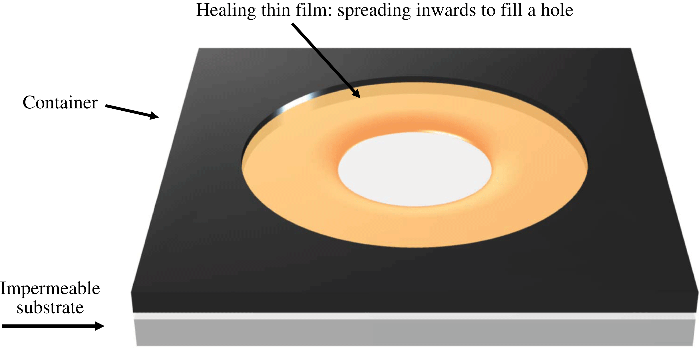
By ‘healing’ of a thin viscous film we refer to the inward spreading of the film to fill a hole or dry spot in the film (see figure 1). Healing films are ubiquitous in a wide spectrum of natural phenomena and technological applications from self-healing to spin coating, and glass transition processes (see e.g. Blossey Reference Blossey2003; Herminghaus, Brinkmann & Seemann Reference Herminghaus, Brinkmann and Seemann2008; Backholm et al. Reference Backholm, Benzaquen, Salez, Raphael and Dalnoki-Veress2014; Dijksman et al. Reference Dijksman, Mukhopadhyay, Gaebler, Witelski and Behringer2015), and the dynamics of axisymmetric holes or dry spots in thin films has been studied extensively from a modelling perspective.
In previous studies, a major focus has been on the stability of the shape of holes of certain size, which is dependent on the relative importance of surface tension, buoyancy (gravity) and contact-line effects (e.g. surface wettability). Moriarty & Schwartz (Reference Moriarty and Schwartz1993) used a lubrication model to investigate the stability and evolution of holes. While, for a non-wetting surface, there may exist an equilibrium hole configuration (Padday Reference Padday1971), this situation is unstable (Sharma & Ruckenstein Reference Sharma and Ruckenstein1990), and the hole will either heal, or expand: either indefinitely, or, in the presence of an outer boundary, until the fluid is collected in a ring near that boundary. In the work of Moriarty & Schwartz (Reference Moriarty and Schwartz1993), advancing and retreating contact angles were prescribed, and the contact line was moved artificially by a mesh point if the angle was greater or less than the advancing or retreating value, respectively (effectively a kind of numerical slip). The stability of holes was also studied by López, Miksis & Bankoff (Reference López, Miksis and Bankoff2001), using the lubrication approximation together with a more natural Navier slip model (along with an assumed contact angle–velocity relation) to regularize the contact-line singularity, instead of the numerical slip that Moriarty & Schwartz (Reference Moriarty and Schwartz1993) implemented, and the numerical results compared favourably to subsequent experimental work (Bankoff et al. Reference Bankoff, Johnson, Miksis, Schluter and López2003).
Schematic of the healing of a thin film, i.e. the inward spreading of a liquid film to fill a ‘hole’ at the centre. Here we focus in the regime when the flow of the thin liquid film is driven by surface tension.
In the present study, our focus is on the thickness profile and contact-line position as a hole heals (see e.g. Diez, Gratton & Gratton Reference Diez, Gratton and Gratton1992; López et al. Reference López, Miksis and Bankoff2001; Zheng, Christov & Stone Reference Zheng, Christov and Stone2014; Dijksman et al. Reference Dijksman, Mukhopadhyay, Gaebler, Witelski and Behringer2015). In this regard, López et al. (Reference López, Miksis and Bankoff2001) adopted a quasi-static approximation, i.e. that the contact-line velocity is much smaller than the time for the thickness profile to reach the quasi-steady balance between gravity and surface tension. Their results compared well with the experiments of Diez et al. (Reference Diez, Gratton and Gratton1992), which were performed in a gravity-dominated parameter regime. In fact, quasi-steadiness is a common assumption in the modelling of spreading droplets and films (Hocking Reference Hocking1983; Savva & Kalliadasis Reference Savva and Kalliadasis2009); however, in the limit of a healing hole, the velocity is (theoretically) unbounded at the time the hole closes, so there is no longer a clear separation of time scales and the quasi-static approximation is no longer valid. We expect this to be particularly true for healing films driven primarily by capillarity, rather than gravity, as the curvature becomes infinite when the hole eventually closes. Thus, instead of modelling the hole-healing dynamics as a quasi-steady process (see e.g. Bostwick, Dijksman & Shearer Reference Bostwick, Dijksman and Shearer2017), we employ an alternate approach, and assume self-similarity in the thickness profile in this study.
We note that self-similar healing films have been studied previously for the case when the flow is driven purely by gravity (Gratton & Minotti Reference Gratton and Minotti1990; Diez et al. Reference Diez, Gratton and Gratton1992), in which a second-order nonlinear diffusion equation describes the time evolution of the interface shape. Also, the gravity-driven healing is analogous to the converging flow processes in a porous medium (or a Hele-Shaw cell) with horizontal heterogeneity (Zheng et al. Reference Zheng, Christov and Stone2014), and the fluid loss effect can be included for healing above a permeable substrate (Zheng, Shin & Stone Reference Zheng, Shin and Stone2015). Although common flows of spreading thin films often admit similarity solutions where the scaling exponents can be identified by dimensional arguments (self-similarity of the first kind), the healing dynamics for a gravity current admits a similarity solution where the scaling exponent is determined from the solution of a nonlinear eigenvalue problem (self-similarity of the second kind) (Barenblatt Reference Barenblatt1979).
For the case of surface-tension-driven flows, as in the present study, the evolution of the interface shape is described by a fourth-order nonlinear partial differential equation (PDE) of the evolution type, that may behave very differently from the nonlinear diffusion equation for gravity-driven flows (see e.g. Voinov Reference Voinov1976; Tanner Reference Tanner1979; Hocking Reference Hocking1983; de Gennes, Hua & Levinson Reference de Gennes, Hua and Levinson1990; Jensen Reference Jensen1994; Oron, Davis & Bankoff Reference Oron, Davis and Bankoff1997; Kalliadasis, Bielarz & Homsy Reference Kalliadasis, Bielarz and Homsy2000; Craster & Matar Reference Craster and Matar2009; Snoeijer & Andreotti Reference Snoeijer and Andreotti2013; Eggers & Fontelos Reference Eggers and Fontelos2015). Here we seek various self-similar solutions for this fourth-order PDE and support our findings via numerical simulations and experiments. We start in § 2 by introducing the theoretical model and deriving the self-similar solutions that develop at different times. In § 3, we report on detailed laboratory-scale experiments for conditions where surface-tension-driven spreading dominates the dynamics. We then compare the theoretical predictions and experimental observations for the front location and the interface shape. In § 4, we present numerical simulations of the original PDE and compare the results with the self-similar solutions. We close the manuscript in § 5 by summarizing the major findings of this work.
2 Theoretical model
2.1 Governing equations
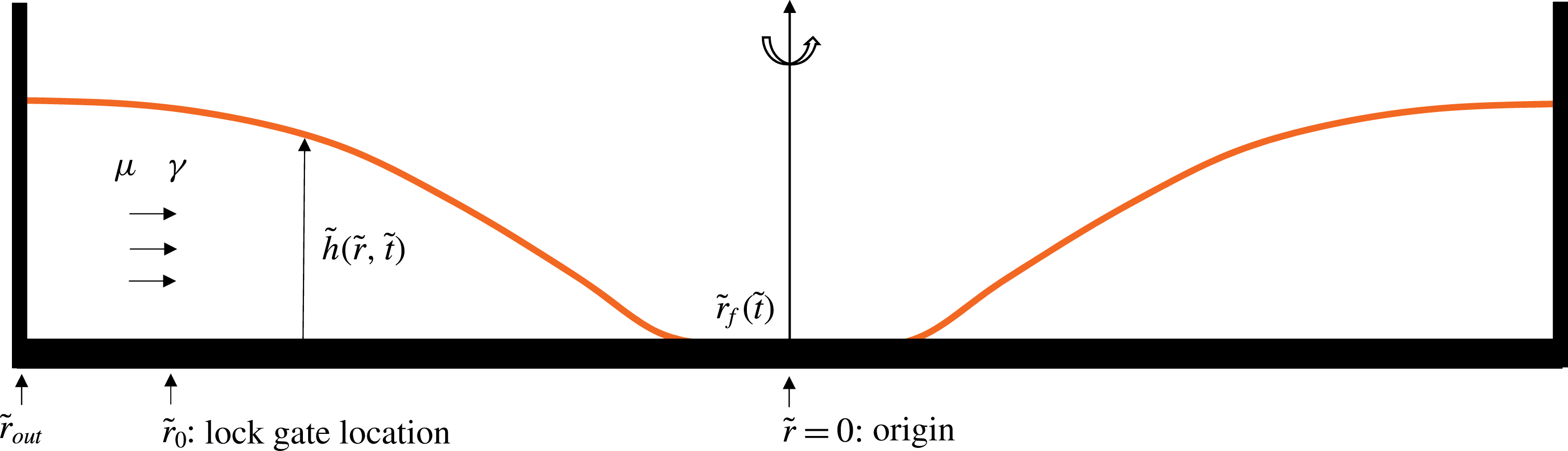
We consider a converging thin-film flow driven by surface tension and assume an axisymmetric geometry, as depicted in figure 2. We assume that the liquid domain is long and thin, and the flow is radial (one-dimensional), so that the lubrication approximation holds. We use
 $\tilde{t}$
,
 $\tilde{r}$
,
 $\unicode[STIX]{x1D707}$
and
 $\unicode[STIX]{x1D6FE}$
to denote time, the radial coordinate, the viscosity of the fluid and surface tension coefficient between air and the spreading fluid, respectively. We also assume that the spreading fluid perfectly wets the substrate so that the contact angle vanishes. Stipulating radial symmetry and neglecting gravitational effects, the governing partial differential equation for the interface shape
 $\tilde{h}\left(\tilde{r},\tilde{t}\right)$
is (e.g. Oron et al.
Reference Oron, Davis and Bankoff1997; Bonn et al.
Reference Bonn, Eggers, Indekeu, Meunier and Rolley2009)
 $$\begin{eqnarray}\frac{\unicode[STIX]{x2202}\tilde{h}}{\unicode[STIX]{x2202}\tilde{t}}+\frac{\unicode[STIX]{x1D6FE}}{3\unicode[STIX]{x1D707}}\frac{1}{\tilde{r}}\frac{\unicode[STIX]{x2202}}{\unicode[STIX]{x2202}\tilde{r}}\left(\tilde{r}\tilde{h}^{3}\frac{\unicode[STIX]{x2202}}{\unicode[STIX]{x2202}\tilde{r}}\left(\frac{1}{\tilde{r}}\frac{\unicode[STIX]{x2202}}{\unicode[STIX]{x2202}\tilde{r}}\left(\tilde{r}\frac{\unicode[STIX]{x2202}\tilde{h}}{\unicode[STIX]{x2202}\tilde{r}}\right)\right)\right)=0.\end{eqnarray}$$
A further assumption is that viscous fluid of height
 $\tilde{h}_{0}$
initially fills the gap between
 $\tilde{r}_{0}$
, the location of a lock gate, and
 $\tilde{r}_{out}$
, the location of a stationary outer boundary. Within the lock gate there is a thin layer of a prewetting liquid film of thickness
 $\tilde{h}_{pw}$
. The introduction of a prewetting film is consistent with our lock-release experiments, as described in § 3, but also with other converging flow situations generated from an instantaneous stop of a rotating container (Dijksman et al.
Reference Dijksman, Mukhopadhyay, Gaebler, Witelski and Behringer2015). In addition, the existence of a prewetting film regularizes the stress singularity at the front. Thus, the initial condition takes the form of
 $$\begin{eqnarray}\tilde{h}\left(\tilde{r},0\right)=\left\{\begin{array}{@{}ll@{}}\tilde{h}_{0},\quad & \tilde{r}_{0}\leqslant \tilde{r}\leqslant \tilde{r}_{out},\\[2.0pt] \tilde{h}_{pw},\quad & 0\leqslant \tilde{r}<\tilde{r}_{0},\end{array}\right.\end{eqnarray}$$
and we are interested in the dynamics of spreading toward the origin (
 $\tilde{r}=0$
). This step initial condition is consistent with our lock-release experiments. We also note that, although the thin-film model equation is strictly speaking valid for small interfacial slopes and is expected to break down when interfacial slopes are large, the step initial condition is rapidly smoothed out to a shape that is appropriate for the thin-film approximation (see e.g. Huppert & Woods Reference Huppert and Woods1995; McGraw et al.
Reference McGraw, Salez, Baumchen, Raphael and Dalnoki-Veress2012).
A healing capillary film: a converging thin viscous film is driven by surface tension. The film thickness is denoted by
 $\tilde{h}(\tilde{r},\tilde{t})$
, while the location of the propagating front is denoted by
 $\tilde{r}_{f}(\tilde{t})$
.
 $\tilde{r}_{0}$
represents the location of a lock gate and
 $\tilde{r}_{out}$
the location of the outer boundary. The viscosity of the fluid and surface tension coefficient are denoted by
 $\unicode[STIX]{x1D707}$
and
 $\unicode[STIX]{x1D6FE}$
, respectively.
To close the problem, we impose the following boundary conditions:
 $$\begin{eqnarray}\frac{\unicode[STIX]{x2202}\tilde{h}}{\unicode[STIX]{x2202}\tilde{r}}=\frac{\unicode[STIX]{x2202}^{3}\tilde{h}}{\unicode[STIX]{x2202}\tilde{r}^{3}}=0\quad \text{at}\;\tilde{r}=0,\quad \text{and}\quad \frac{\unicode[STIX]{x2202}\tilde{h}}{\unicode[STIX]{x2202}\tilde{r}}=\frac{\unicode[STIX]{x2202}}{\unicode[STIX]{x2202}\tilde{r}}\left(\frac{1}{\tilde{r}}\frac{\unicode[STIX]{x2202}}{\unicode[STIX]{x2202}\tilde{r}}\left(\tilde{r}\frac{\unicode[STIX]{x2202}\tilde{h}}{\unicode[STIX]{x2202}\tilde{r}}\right)\right)=0\quad \text{at}\;\tilde{r}=\tilde{r}_{out}.\end{eqnarray}$$
The first pair of these are symmetry conditions applied at the centre of the domain, while the second pair are, respectively,
 $90^{\circ }$
contact-angle and zero-flux conditions at the outer wall (see e.g. López et al. (Reference López, Miksis and Bankoff2001) for a discussion of the outer contact-angle condition).
Next, we define dimensionless variables
 $h\equiv \tilde{h}/\tilde{h}_{0}$
,
 $r\equiv \tilde{r}/\tilde{r}_{0}$
and
 $t\equiv \tilde{t}/\tilde{t}_{c}$
, where the characteristic time is chosen as
 $$\begin{eqnarray}\tilde{t}_{c}=\frac{3\unicode[STIX]{x1D707}\tilde{r}_{0}^{4}}{\unicode[STIX]{x1D6FE}\tilde{h}_{0}^{3}},\end{eqnarray}$$
and obtain the dimensionless form of (2.1):
 $$\begin{eqnarray}\frac{\unicode[STIX]{x2202}h}{\unicode[STIX]{x2202}t}+\frac{1}{r}\frac{\unicode[STIX]{x2202}}{\unicode[STIX]{x2202}r}\left(rh^{3}\frac{\unicode[STIX]{x2202}}{\unicode[STIX]{x2202}r}\left(\frac{1}{r}\frac{\unicode[STIX]{x2202}}{\unicode[STIX]{x2202}r}\left(r\frac{\unicode[STIX]{x2202}h}{\unicode[STIX]{x2202}r}\right)\right)\right)=0.\end{eqnarray}$$
The dimensionless initial condition (2.2) becomes
 $$\begin{eqnarray}h\left(r,0\right)=\left\{\begin{array}{@{}ll@{}}1,\quad & 1\leqslant r\leqslant r_{out},\\ h_{pw},\quad & 0\leqslant r<1,\end{array}\right.\end{eqnarray}$$
where
 $h_{pw}\equiv \tilde{h}_{pw}/\tilde{h}_{0}\ll 1$
and
 $r_{out}\equiv \tilde{r}_{out}/\tilde{r}_{0}\gg 1$
, and the dimensionless boundary conditions (2.3) become
 $$\begin{eqnarray}\frac{\unicode[STIX]{x2202}h}{\unicode[STIX]{x2202}r}=\frac{\unicode[STIX]{x2202}^{3}h}{\unicode[STIX]{x2202}r^{3}}=0\quad \text{at }r=0,\quad \text{and}\quad \frac{\unicode[STIX]{x2202}h}{\unicode[STIX]{x2202}r}=\frac{\unicode[STIX]{x2202}}{\unicode[STIX]{x2202}r}\left(\frac{1}{r}\frac{\unicode[STIX]{x2202}}{\unicode[STIX]{x2202}r}\left(r\frac{\unicode[STIX]{x2202}h}{\unicode[STIX]{x2202}r}\right)\right)=0\quad \text{at }r=r_{out}.\end{eqnarray}$$
Equation (2.5) is solved subject to the initial and boundary conditions (2.6), (2.7) and provides the time evolution of the profile shape
 $h(r,t)$
.
While the main focus of this study is on the behaviour of the film close to the time when it heals, it is also interesting to analyse the early-time relaxation process. We provide a self-similar solution in appendix A for the early-time relaxation dynamics from the initial step condition (2.6).
2.2 Similarity transform
We now focus on the late-time dynamics as the hole closes, i.e. as
 $r_{f}(t)\rightarrow 0$
. We use
 $t_{0}$
to denote the dimensionless healing time, that is, the time for the (circular) front of the air–fluid interface to reach the origin (
 $r=0$
), and we look for a self-similar solution for equation (2.5) of the form
 $$\begin{eqnarray}h(r,t)=(t_{0}-t)^{\unicode[STIX]{x1D6FC}}f\left(\unicode[STIX]{x1D709}\right),\quad \text{where }\unicode[STIX]{x1D709}\equiv \frac{r}{(t_{0}-t)^{\unicode[STIX]{x1D6FD}}}.\end{eqnarray}$$
From dimensional analysis and (2.5), we obtain the following relationship between the exponents
 $$\begin{eqnarray}\unicode[STIX]{x1D6FC}=\frac{(4\unicode[STIX]{x1D6FD}-1)}{3}.\end{eqnarray}$$
We can then rewrite (2.5) as an ordinary differential equation (ODE):
 $$\begin{eqnarray}-\frac{(4\unicode[STIX]{x1D6FD}-1)}{3}f+\unicode[STIX]{x1D6FD}\unicode[STIX]{x1D709}\frac{\text{d}f}{\text{d}\unicode[STIX]{x1D709}}+\frac{1}{\unicode[STIX]{x1D709}}\frac{\text{d}}{\text{d}\unicode[STIX]{x1D709}}\left(\unicode[STIX]{x1D709}f^{3}\frac{\text{d}}{\text{d}\unicode[STIX]{x1D709}}\left(\frac{1}{\unicode[STIX]{x1D709}}\frac{\text{d}}{\text{d}\unicode[STIX]{x1D709}}\left(\unicode[STIX]{x1D709}\frac{\text{d}f}{\text{d}\unicode[STIX]{x1D709}}\right)\right)\right)=0,\end{eqnarray}$$
where the exponent
 $\unicode[STIX]{x1D6FD}$
is as yet undetermined.
2.2.1 Far-field condition
Appropriate boundary conditions are needed to solve (2.10) for the interface shape
 $f(\unicode[STIX]{x1D709})$
and determine parameter
 $\unicode[STIX]{x1D6FD}$
. The similarity solution will not hold everywhere in
 $r$
and
 $t$
, but rather, in a region near the apparent contact line, for time sufficiently close to
 $t_{0}$
. Since
 $\unicode[STIX]{x1D709}\rightarrow \infty$
for fixed
 $r$
as
 $t\rightarrow 0$
, the similarity solution is defined on the semi-infinite domain
 $0<\unicode[STIX]{x1D709}<\infty$
.
The rate of change of film thickness
 $\unicode[STIX]{x2202}h/\unicode[STIX]{x2202}t$
blows up as
 $(t_{0}-t)^{\unicode[STIX]{x1D6FC}-1}$
. However, we expect
 $\unicode[STIX]{x2202}h/\unicode[STIX]{x2202}t$
to remain bounded away from the middle of the hole, which requires the first two terms in (2.10) to balance. This gives the far-field ‘quasi-stationarity’ condition
 $$\begin{eqnarray}-\frac{(4\unicode[STIX]{x1D6FD}-1)}{3}f+\unicode[STIX]{x1D6FD}\unicode[STIX]{x1D709}\frac{\text{d}f}{\text{d}\unicode[STIX]{x1D709}}\rightarrow 0\quad \text{as}\;\unicode[STIX]{x1D709}\rightarrow \infty .\end{eqnarray}$$
Solving this equation provides
 $$\begin{eqnarray}f(\unicode[STIX]{x1D709})\sim a_{1}\unicode[STIX]{x1D709}^{(4\unicode[STIX]{x1D6FD}-1)/(3\unicode[STIX]{x1D6FD})}\quad \text{as}\;\unicode[STIX]{x1D709}\rightarrow \infty .\end{eqnarray}$$
This kind of condition has been employed previously in studying other problems involving the formation of finite-time singularities such as the capillary-driven breakup of viscous threads (see e.g. Eggers Reference Eggers1993; Papageorgiou Reference Papageorgiou1995; Brenner, Lister & Stone Reference Brenner, Lister and Stone1996; Lister & Stone Reference Lister and Stone1998; Eggers & Fontelos Reference Eggers and Fontelos2009), and the van der Waals-driven rupture of thin films (see e.g. Witelski & Bernoff Reference Witelski and Bernoff1999; Zhang & Lister Reference Zhang and Lister1999; Dallaston et al. Reference Dallaston, Tseluiko, Zheng, Fontelos and Kalliadasis2017).
2.2.2 Near-field condition
ODE (2.10) permits a number of different near-field behaviours, as either
 $\unicode[STIX]{x1D709}$
or
 $f$
approaches zero. However, only particular solutions will exhibit behaviour that can be matched to a prewetting film. Assume that
 $f$
becomes small at an apparent contact line
 $\unicode[STIX]{x1D709}=\unicode[STIX]{x1D709}_{0}>0$
, while
 $f^{\prime }\equiv \text{d}f/\text{d}\unicode[STIX]{x1D709}$
remains of order unity: the dominant terms in (2.10) in an ‘inner region’ near the contact line are
 $\unicode[STIX]{x1D6FD}\unicode[STIX]{x1D709}_{0}f^{\prime }+(f^{3}f^{\prime \prime \prime })^{\prime }=0$
, which can be integrated once to give
 $$\begin{eqnarray}\unicode[STIX]{x1D6FD}\unicode[STIX]{x1D709}_{0}\,f+f^{3}\frac{\text{d}^{3}f}{\text{d}\unicode[STIX]{x1D709}^{3}}=\unicode[STIX]{x1D716}.\end{eqnarray}$$
If
 $f$
goes to zero it must do so as
 $f\sim c_{1}(\unicode[STIX]{x1D709}-\unicode[STIX]{x1D709}_{0})^{3/4}$
, which is unphysical and cannot match to a thin prewetting film. However, (2.13) also has solutions with a thin prewetting film
 $f\sim f_{pw}=\unicode[STIX]{x1D716}/(\unicode[STIX]{x1D6FD}\unicode[STIX]{x1D709}_{0})>0$
for
 $\unicode[STIX]{x1D709}\ll \unicode[STIX]{x1D709}_{0}$
(Landau & Levich Reference Landau and Levich1942; Myers Reference Myers1998). We will find below that there is only one such solution to (2.10) that has such a film for any given
 $\unicode[STIX]{x1D6FD}$
, once certain scale invariances have been accounted for. An expanded account on all the possible near-field behaviours is presented in § C.3.
2.3 Self-similar solutions for general exponent
 $\unicode[STIX]{x1D6FD}$

2.3.1 Shooting procedure
To compute the self-similar solutions for ODE (2.10), a shooting procedure can be used from a large value of
 $\unicode[STIX]{x1D709}$
, representing the far field, toward the contact line. For example, when
 $\unicode[STIX]{x1D6FD}=2/5$
, the far-field behaviour of
 $f(\unicode[STIX]{x1D709})$
has a relatively simple form (with details provided in appendix B)
 $$\begin{eqnarray}f(\unicode[STIX]{x1D709})\sim a_{1}\unicode[STIX]{x1D709}^{1/2}+a_{2}\unicode[STIX]{x1D709}^{-8/5}\text{e}^{-6/5\left(2/5\right)^{1/3}a_{1}^{-1}\unicode[STIX]{x1D709}^{5/6}}+O(1)\quad \text{as}\,\unicode[STIX]{x1D709}\rightarrow \infty ,\end{eqnarray}$$
where
 $a_{1}$
and
 $a_{2}$
are two free parameters. Thus, by specifying the values of
 $a_{1}$
and
 $a_{2}$
, we can obtain the values of
 $f$
and its derivatives at a far-field location that can be used in the shooting procedure. We note, however, that since (2.10) is invariant under the transformation
 $f\mapsto \unicode[STIX]{x1D706}f$
,
 $\unicode[STIX]{x1D709}\mapsto \unicode[STIX]{x1D706}^{3/4}\unicode[STIX]{x1D709}$
, where
 $\unicode[STIX]{x1D706}$
is a positive constant, we may set
 $a_{1}=1$
without loss of generality, and, by varying
 $a_{2}$
, construct the one-parameter family of solutions that are unique up to such a rescaling.
In figure 3, we show representative solutions of (2.10) for
 $\unicode[STIX]{x1D6FD}=2/5$
, computed using the described shooting procedure. In all the cases, we start from a far-field location
 $\unicode[STIX]{x1D709}_{\infty }=10$
, and shoot toward the origin using the MATLAB subroutine ODE45. Initial conditions are provided by setting
 $a_{1}=1$
and varying the values of
 $a_{2}$
from
 $-10$
to
 $10$
. From figure 3, we observe five distinct near-field behaviours as
 $a_{2}$
varies: blow-up, generic touch-down, touch-down at the origin, a thick film and a non-generic solution that separates the generic touch-down solutions from the blow-up ones. It is this non-generic solution that has the appropriate structure near an apparent contact line, as we see next.
Representative solutions of (2.10) with similarity exponent
 $\unicode[STIX]{x1D6FD}=2/5$
using a shooting procedure from a far-field location. In all cases,
 $a_{1}=1$
and the far-field location is chosen as
 $\unicode[STIX]{x1D709}_{\infty }=10$
. Consistent with the asymptotic analysis for the near-field behaviour, five different scenarios have been observed as is indicated in the legend: blow-up, generic touch-down, touch-down at the origin, a thick film and a non-generic critical solution that represents the crossover between generic touch-down and blow-up solutions (see appendix C for details). The inset is a semi-log plot of the figure, which highlights the near-field behaviours. The non-generic solution corresponds to the interface shape of the healing capillary film problem.

2.3.2 Alternative procedures
In principle, we can compute numerical solutions to ODE (2.10) for a range of
 $\unicode[STIX]{x1D6FD}$
values, and vary
 $a_{2}$
to find the critical solution between blow-up and touch-down. For
 $\unicode[STIX]{x1D6FD}\neq 2/5$
, however, there is an infinite series of algebraic terms in the far-field behaviour, and so it is much harder to set the prefactor on the exponential, e.g.
 $a_{2}$
in (2.14), numerically. As an alternative, we handle the far field for general
 $\unicode[STIX]{x1D6FD}$
by posing a suitable boundary-value problem on the interval
 $[\unicode[STIX]{x1D709}_{\infty }/2,\unicode[STIX]{x1D709}_{\infty }]$
, where
 $\unicode[STIX]{x1D709}_{\infty }\gg 1$
represents a far-field location, and then solving an initial-value problem on
 $[0,\unicode[STIX]{x1D709}_{\infty }/2]$
from
 $\unicode[STIX]{x1D709}=\unicode[STIX]{x1D709}_{\infty }/2$
toward
 $\unicode[STIX]{x1D709}=0$
(the origin). In particular, the following conditions are employed for the boundary-value problem on
 $[\unicode[STIX]{x1D709}_{\infty }/2,\unicode[STIX]{x1D709}_{\infty }]$
:
 $$\begin{eqnarray}\displaystyle & \displaystyle -\frac{4\unicode[STIX]{x1D6FD}-1}{3}f+\unicode[STIX]{x1D6FD}\unicode[STIX]{x1D709}\frac{\text{d}f}{\text{d}\unicode[STIX]{x1D709}}=0,\quad f=\unicode[STIX]{x1D709}^{(4\unicode[STIX]{x1D6FD}-1)/3\unicode[STIX]{x1D6FD}}\quad \text{at}\;\unicode[STIX]{x1D709}=\unicode[STIX]{x1D709}_{\infty }, & \displaystyle\end{eqnarray}$$
 $$\begin{eqnarray}\displaystyle & \displaystyle -\frac{4\unicode[STIX]{x1D6FD}-1}{3}f+\unicode[STIX]{x1D6FD}\unicode[STIX]{x1D709}\frac{\text{d}f}{\text{d}\unicode[STIX]{x1D709}}=0,\quad f=B\quad \text{at}\;\unicode[STIX]{x1D709}=\frac{\unicode[STIX]{x1D709}_{\infty }}{2}, & \displaystyle\end{eqnarray}$$
 $B$
is a free parameter. Then, four initial conditions (
 $f,f^{\prime },f^{\prime \prime },f^{\prime \prime \prime }$
) can be provided at
 $\unicode[STIX]{x1D709}=\unicode[STIX]{x1D709}_{\infty }/2$
, and an initial-value problem can be solved toward the origin. Different values of
 $B$
correspond to different values of
 $a_{1}$
in (2.14), thus generating different solutions such as the generic touch-down, non-generic thin-film and blow-up solutions, analogous to the different scenarios identified for
 $\unicode[STIX]{x1D6FD}=2/5$
in figure 3. As a check on our handling of the far field, for
 $\unicode[STIX]{x1D6FD}=2/5$
the non-generic touch-down solution obtained using this method (shown in figure 4
a) is indistinguishable from the corresponding solution obtained using the shooting procedure with far-field condition (2.14). In order to resolve the features of the solution near
 $f=0$
, we used an adaptive ODE solver with a precision of up to thirty digits, implemented in the computer algebra system MAPLE.
Self-similar solutions in the contact-line-dominated regime with general values of
 $\unicode[STIX]{x1D6FD}$
. (a) Profile shapes for
 $\unicode[STIX]{x1D6FD}=$
 $0.40$
,
 $0.42$
,
 $0.44$
,
 $0.46$
,
 $0.48$
,
 $0.50$
. The slope in the far field increases when
 $\unicode[STIX]{x1D6FD}$
increases. Inset: taking
 $\unicode[STIX]{x1D6FD}=0.50$
as an example, numerical solutions show that a thin prewetting film develops near the contact line. (b) The influence of
 $\unicode[STIX]{x1D6FD}$
on the thickness of the prewetting film
 $f_{pw}$
developed toward the origin. The film thickness
 $f_{pw}$
ranges from
 $O(10^{-4})$
for
 $\unicode[STIX]{x1D6FD}=0.50$
to
 $O(10^{-21})$
for
 $\unicode[STIX]{x1D6FD}=0.40$
. In all cases, a representative far-field location is chosen as
 $\unicode[STIX]{x1D709}_{\infty }=10$
.

We show in figure 4(a) representative self-similar solutions for
 $\unicode[STIX]{x1D6FD}=$
 $0.40$
,
 $0.42$
,
 $0.44$
,
 $0.46$
,
 $0.48$
,
 $0.50$
. By varying
 $B$
, we approach the non-generic solution in which a thin prewetting film is present, instead of a front (
 $f=0$
) near the contact line. The film thickness
 $f_{pw}$
ranges from
 $O(10^{-4})$
for
 $\unicode[STIX]{x1D6FD}=0.50$
to
 $O(10^{-21})$
for
 $\unicode[STIX]{x1D6FD}=0.40$
, as shown in figure 4(b). In this case, we can define the apparent front location
 $\unicode[STIX]{x1D709}_{f}$
as the location of the local minimum of the profile shapes, by which
 $\unicode[STIX]{x1D709}_{f}\approx 0.245$
for
 $\unicode[STIX]{x1D6FD}=0.40$
. Here we distinguish between
 $\unicode[STIX]{x1D709}_{f}$
, the location of the apparent contact line, and
 $\unicode[STIX]{x1D709}_{0}$
, the actual touch-down point for any given generic solution.
We note that numerical solutions for ODE (2.10) can also be computed by solving the associated two-point boundary-value problem using numerical continuation, as another alternative procedure. We have carried this out for the case of generic touch-down solutions, with details in appendix D, and the results agree well with the solutions of the shooting procedure, particularly the relationship between
 $\unicode[STIX]{x1D6FD}$
and
 $f_{pw}$
depicted in figure 4(b).
2.3.3 Determining
$\unicode[STIX]{x1D6FD}$
from the prewetting film thickness

The presence of a continuum of self-similar solutions with regard to parameter
 $\unicode[STIX]{x1D6FD}$
raises the question how a particular value of
 $\unicode[STIX]{x1D6FD}$
is chosen for a given prewetting film thickness
 $h_{pw}$
. Although there is a clear relationship between
 $\unicode[STIX]{x1D6FD}$
and the scaled prewetting thickness
 $f_{pw}$
, a constant value of
 $h_{pw}$
, arising from the initial condition (2.6), implies a varying value of
 $f_{pw}$
, and from the scaling (2.8), the connection is given by
 $$\begin{eqnarray}h_{pw}=(t_{0}-t)^{(4\unicode[STIX]{x1D6FD}-1)/3}f_{pw}.\end{eqnarray}$$
Since
 $f_{pw}$
depends on
 $\unicode[STIX]{x1D6FD}$
, as illustrated in figure 4(b), equation (2.16) can be viewed as an equation for
 $\unicode[STIX]{x1D6FD}$
as a function of a logarithmic time variable
 $\unicode[STIX]{x1D70F}\equiv -\log (t_{0}-t)$
. By taking
 $\log$
on both sides of (2.16), we obtain
 $$\begin{eqnarray}\log h_{pw}=-\frac{4\unicode[STIX]{x1D6FD}-1}{3}\unicode[STIX]{x1D70F}+\log f_{pw}(\unicode[STIX]{x1D6FD}),\end{eqnarray}$$
which yields, upon differentiation with respect to
 $\unicode[STIX]{x1D70F}$
,
 $$\begin{eqnarray}\left(-\frac{4}{3}\unicode[STIX]{x1D70F}+\frac{\text{d}}{\text{d}\unicode[STIX]{x1D6FD}}\log f_{pw}(\unicode[STIX]{x1D6FD})\right)\frac{\text{d}\unicode[STIX]{x1D6FD}}{\text{d}\unicode[STIX]{x1D70F}}=\frac{4\unicode[STIX]{x1D6FD}-1}{3},\end{eqnarray}$$
and hence
 $$\begin{eqnarray}\frac{\text{d}\unicode[STIX]{x1D6FD}}{\text{d}\unicode[STIX]{x1D70F}}=\frac{4\unicode[STIX]{x1D6FD}-1}{\left(-4\unicode[STIX]{x1D70F}+3\displaystyle \frac{\text{d}}{\text{d}\unicode[STIX]{x1D6FD}}\log f_{pw}(\unicode[STIX]{x1D6FD})\right)}.\end{eqnarray}$$
We must therefore think of
 $\unicode[STIX]{x1D6FD}$
as slowly changing in time, thus our solutions are only ‘quasi’-self-similar in nature. However, the very fast variation of
 $f_{pw}(\unicode[STIX]{x1D6FD})$
, with
 $\unicode[STIX]{x1D6FD}$
depicted in figure 4(b), suggests that
 $\text{d}/\text{d}\unicode[STIX]{x1D6FD}\log f_{pw}(\unicode[STIX]{x1D6FD})=O(10^{2})$
, which results in a small right-hand side in (2.19), i.e.
 $\text{d}\unicode[STIX]{x1D6FD}/\text{d}\unicode[STIX]{x1D70F}=O(10^{-2})$
. Thus, the change in
 $\unicode[STIX]{x1D6FD}$
will be small when
 $\unicode[STIX]{x1D70F}$
only changes a few units, i.e. when
 $(t_{0}-t)$
only changes for a few decades, which is usually the case in both experiments and numerical simulations.
A more rigorous approach requires an adiabatic approximation, where we write
 $h(r,t)=(t_{0}-t)^{(4\unicode[STIX]{x1D6FD}(\unicode[STIX]{x1D70F})-1)/3}f(\unicode[STIX]{x1D70F},\unicode[STIX]{x1D709})$
, and
 $f(\unicode[STIX]{x1D70F},\unicode[STIX]{x1D709})$
satisfies the following equation:
 $$\begin{eqnarray}\frac{\unicode[STIX]{x2202}f}{\unicode[STIX]{x2202}\unicode[STIX]{x1D70F}}+\text{e}^{-\unicode[STIX]{x1D70F}}\!\left(\frac{4}{3}f-\unicode[STIX]{x1D709}\frac{\unicode[STIX]{x2202}f}{\unicode[STIX]{x2202}\unicode[STIX]{x1D709}}\right)\!\frac{\text{d}\unicode[STIX]{x1D6FD}}{\text{d}\unicode[STIX]{x1D70F}}-\frac{(4\unicode[STIX]{x1D6FD}-1)}{3}f+\unicode[STIX]{x1D6FD}\unicode[STIX]{x1D709}\frac{\unicode[STIX]{x2202}f}{\unicode[STIX]{x2202}\unicode[STIX]{x1D709}}+\frac{1}{\unicode[STIX]{x1D709}}\frac{\unicode[STIX]{x2202}}{\unicode[STIX]{x2202}\unicode[STIX]{x1D709}}\!\left(\unicode[STIX]{x1D709}f^{3}\frac{\unicode[STIX]{x2202}}{\unicode[STIX]{x2202}\unicode[STIX]{x1D709}}\left(\frac{1}{\unicode[STIX]{x1D709}}\frac{\unicode[STIX]{x2202}}{\unicode[STIX]{x2202}\unicode[STIX]{x1D709}}\left(\unicode[STIX]{x1D709}\frac{\unicode[STIX]{x2202}f}{\unicode[STIX]{x2202}\unicode[STIX]{x1D709}}\right)\!\right)\!\right)=0.\end{eqnarray}$$
After neglecting the terms associated with
 $\text{d}\unicode[STIX]{x1D6FD}/\text{d}\unicode[STIX]{x1D70F}$
and
 $\unicode[STIX]{x2202}f/\unicode[STIX]{x2202}\unicode[STIX]{x1D70F}$
, we recover equation (2.10) for the similarity solutions, except that now
 $\unicode[STIX]{x1D6FD}(\unicode[STIX]{x1D70F})$
is a slowly varying parameter evolving according to (2.19).
Given the exponent
 $(4\unicode[STIX]{x1D6FD}-1)/3<1$
, the factor
 $(t_{0}-t)^{(4\unicode[STIX]{x1D6FD}-1)/3}$
in (2.16) is of
 $O(1)$
, so the order of magnitudes of
 $f_{pw}$
and
 $h_{pw}$
will match except for when
 $t$
is very close to
 $t_{0}$
. From an experimental perspective, we will observe an apparent power law (thus a value for
 $\unicode[STIX]{x1D6FD}$
), from which we can derive an appropriate order of magnitude for
 $f_{pw}$
and hence
 $h_{pw}$
through the curve in figure 4(b). In other words, once
 $h_{pw}$
is provided in an experiment or numerical simulation, a corresponding scaling exponent
 $\unicode[STIX]{x1D6FD}$
will be observed.
2.3.4 The special value
$\unicode[STIX]{x1D6FD}=2/5$

As well as producing the convenient far-field behaviour (2.14), the value
 $\unicode[STIX]{x1D6FD}=2/5$
also has the property of exhibiting a constant, non-zero flow rate far from the front of a healing film. A non-zero flow rate must be sustained away from the hole during the healing process in order to fill the hole with liquid. Setting the flow rate to be constant, or equivalently,
 $\unicode[STIX]{x2202}h/\unicode[STIX]{x2202}t=0$
, in (2.5), we obtain the interface shape in the far field
 $$\begin{eqnarray}h\propto r^{1/2}\quad \text{for }r\gg r_{f}(t).\end{eqnarray}$$
We note that we have neglected the solutions behaving as
 $h\propto r^{2}$
and as
 $h\propto \ln r$
in the far field, since these solutions correspond to zero flux, whereas the asymptotic behaviour given by (2.21) corresponds to a time-independent flow rate in the far field
 $$\begin{eqnarray}F\equiv 2\unicode[STIX]{x03C0}rh^{3}\frac{\text{d}}{\text{d}r}\left(\frac{1}{r}\frac{\text{d}}{\text{d}r}\left(r\frac{\text{d}h}{\text{d}r}\right)\right)\!.\end{eqnarray}$$
Thus, the equivalent far-field behaviour in the self-similar solutions has
 $f\propto \unicode[STIX]{x1D709}^{1/2}$
, which corresponds to the value
 $\unicode[STIX]{x1D6FD}=2/5$
. We will see some experimental and computational evidence in §§ 3 and 4 that the exponent
 $\unicode[STIX]{x1D6FD}=2/5$
influences the profile shape of the film away from the contact line.
3 Experimental observations
In this section, we describe our laboratory experiments of inward spreading liquid films and compare the experimentally obtained time-dependent front locations and profile shapes with the self-similar solutions from the theoretical model (§ 2).
3.1 Experimental set-up and calibration
A schematic of our experimental set-up is depicted in figure 5(a). We first prepare a clean oil-wetting slide glass as a flat substrate, with an LED panel placed below to provide a uniform back lighting. We then place a rubber container above the slide glass to form a circular outer boundary. A rubber cylinder, as a cylindrical lock gate, is then placed at the centre of the circular area surrounded by the outer boundary. A digital camera (Nikon 7100) or an inverted fluorescence microscope (DMI4000B, Leica) is placed above the set-up, and photographs are taken from the top. The microscope has a smaller range (0
 ${\leqslant}\tilde{r}\leqslant$
2.5 mm) but a much higher resolution, so is used to measure the profile shape evolution when the hole is small.
Experimental set-up to measure the front location and film thickness of healing liquid films. (a) A camera or a microscope is placed at the top of the inwardly spreading liquid film. A small amount of dye is added to the liquid film. (b) A representative image taken by the digital camera, using silicone oil (500 cSt) as the spreading liquid. The difference in the colour intensity indicates the difference in the film thickness at different locations. (c) The profile shape (along the straight line I–II of panel b) can be reconstructed based on a calibration that links the intensity with the film thickness.

In each experiment, we first fill the gap between the lock gate (rubber cylinder) and the outer boundary (rubber container) with a viscous fluid. We use silicone oils with different viscosities (e.g. Sigma-Aldrich: 20 cSt, 100 cSt, 500 cSt) as the working fluids in our experiments, which do not wet the lock gate and the outer boundary significantly. However, the silicone oils wet the substrate (slide glass), and we expect the existence of a prewetting film. Upon the removal of the lock gate, the liquid spreads inward, filling the hole at the centre. The initial film thickness is chosen to be less than 1 mm. A representative picture (top view) taken by the camera is shown in figure 5(b). The front of the liquid film is approximately circular, and we can measure the radius of the circular front
 $\tilde{r}_{f}(\tilde{t})$
as a function of time,
 $\tilde{t}$
.
Calibration experiments: (a) experimental set-up; (b) calibration curve. A tapered cell filled with dyed liquid was used for the calibration experiments, for example. A representative image (top view) is shown in (a), which indicates an intensity change as the thickness of the dyed liquid varies. The relationship between the liquid thickness and image intensity is shown in (b), and a linear fit is used for the data analysis.

Time-dependent images of the inward spreading films in two different experiments: (a) silicone oil 500 cSt (experiment 1 in table 1), and (b) silicone oil 20 cSt (not shown in table 1). The front location is indicated with the dashed line. In both experiments, we kept the same locations for the lock gate (
 $\tilde{r}_{0}\approx 6.4$
mm) and the outer boundary (
 $\tilde{r}_{out}\approx 16.7$
mm). The initial film thickness is (a)
 $\tilde{h}_{0}\approx 0.65$
mm, and (b)
 $\tilde{h}_{0}\approx 0.4$
mm.

A summary of the parameters of the different experiments is given in table 1. To measure the interface shape, we add a small amount of dye (Sigma-Aldrich: Sudan III) to the silicone oils. The dye and silicone oils are well mixed, and the presence of the dye does not significantly change the viscosity and surface tension. As a result, different film thicknesses correspond to different signal intensities received by the digital camera (see e.g. Bischofberger, Ramachandran & Nagel Reference Bischofberger, Ramachandran and Nagel2014). In addition, we are able to conduct a careful calibration that relates the film thickness to the intensity of the image taken by the digital camera or the microscope; see figure 6 as an example. Then, in our post-experimental data analysis, we reconstruct the profile shapes
 $\tilde{h}(\tilde{r},\tilde{t})$
at different times
 $\tilde{t}$
. A representative profile shape is shown in figure 5(c), which corresponds to the images displayed in figure 5(b).
Summary of the parameters of the different experiments that we performed of viscous thin films propagating inwards to fill a hole. We note that we verified that the addition of small amount of dye (Sudan III) does not influence the physical properties such as viscosity, density and surface tension. The viscosity values in this table are provided from the manufacturer.
 $\tilde{t}_{0}$
corresponds to the time when the front reaches the origin.

Time-dependent front locations from the experimental measurements: (a) raw data and (b) rescaled experimental data. The initial film thickness is chosen to be smaller than or equal to 0.8 mm in this figure. A nonlinear power-law fit of the data in the range
 $0.01\leqslant r_{f}(t)\leqslant 0.2$
provides an exponent of
 $\unicode[STIX]{x1D6FD}=0.489\pm 0.045$
. The slopes of
 $2/5$
and 0.49 in the log–log graph are also shown as straight lines for reference.

3.2 Front location
As we mentioned above, the time evolution of the location of the propagating front can be obtained from the top view still images, using a digital camera. Typical experimental results showing the closing of the initial hole are shown in figure 7. We note that a drift can occur in some experiments, as can be seen, for example, in figure 7(b). However, in all the experiments, the propagating front appears circular as time progresses, which allows us to define the front location
 $\tilde{r}_{f}(t)$
based on the radius of the circle, and relocate the origin
 $\tilde{r}=0$
at the centre of the circle. In addition, in each experiment, there exists a critical time
 $\tilde{t}_{0}$
at which the front reaches the origin, i.e. when
 $\tilde{r}_{f}=0$
. Equivalently,
 $\tilde{t}_{0}-\tilde{t}$
represents the time that remains for the front to reach the origin.
The experimental data of
 $\tilde{r}_{f}$
versus
 $\tilde{t}_{0}-\tilde{t}$
are shown in figure 8(a). We also present the non-dimensionalized experimental data of the front location in figure 8(b). We impose a nonlinear power-law fit for the experimental data in the range
 $0.01\leqslant r_{f}(t)\leqslant 0.2$
, which provides an exponent of
 $0.489\pm 0.045$
. It is noteworthy that the similarity exponent
 $\unicode[STIX]{x1D6FD}\approx 0.49$
corresponds to a value of prewetting thickness
 $f_{pw}$
(and hence
 $h_{pw}$
, as argued in § 2.3.3) of
 $O(10^{-5})$
. In addition,
 $h_{pw}$
of
 $O(10^{-5})$
corresponds to
 $\tilde{h}_{pw}$
of
 $O(10)$
nm in our experiments, which is consistent with the typical order of the surface roughness of the substrate (glass slide) and also the typical thickness of prewetting films (see e.g. Bonn et al.
Reference Bonn, Eggers, Indekeu, Meunier and Rolley2009). In addition, we note that the observed power law is consistent with the power-law data fitting results of the related converging flow experiments and numerical computations of Dijksman et al. (Reference Dijksman, Mukhopadhyay, Gaebler, Witelski and Behringer2015).
3.3 Profile shapes
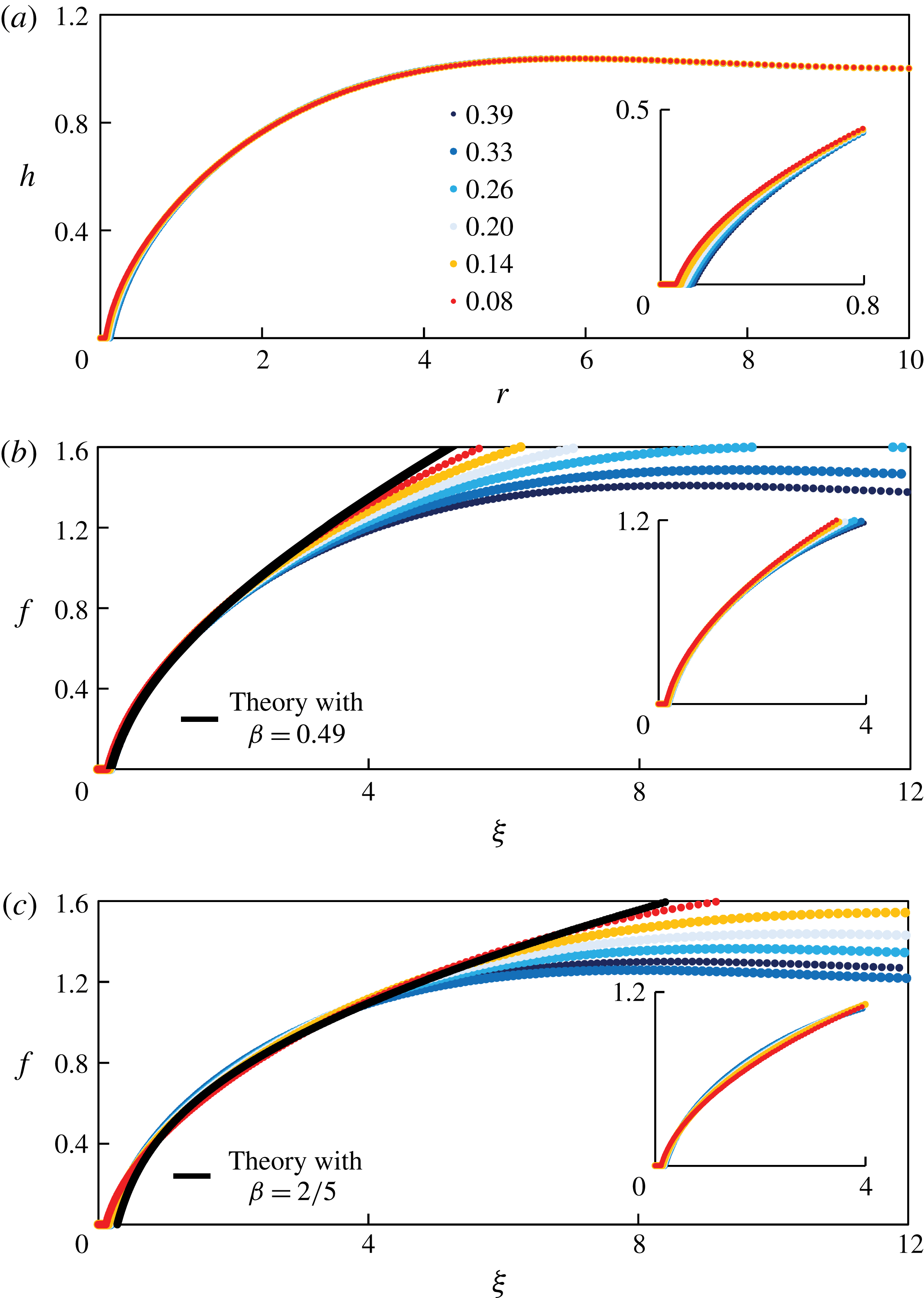
Using an inverted fluorescence microscope, we are able to measure the spatiotemporal evolution of the profile shapes in our experiments. The time-dependent profile shapes from a representative experiment (experiment 1 in table 1) are shown in figure 9(a), where silicone oil of viscosity
 $\unicode[STIX]{x1D707}\approx 500$
cSt and surface tension
 $\unicode[STIX]{x1D6FE}\approx 20.2~\text{mN}~\text{m}^{-1}$
was used.
We then rescale the profile shapes based on the self-similar solution with
 $\unicode[STIX]{x1D6FD}=0.49$
, as shown in figure 9(b), and we observe excellent data collapse in the region close to the contact line. The theoretical prediction with
 $\unicode[STIX]{x1D6FD}=0.49$
is also plotted as the black curve in figure 9(b), and is found to agree well with collapsed profiles from experimental measurements. The collapse of profile shapes at different times and the agreement with self-similar solutions have not been reported in previous experimental studies on converging films (see e.g. Dijksman et al.
Reference Dijksman, Mukhopadhyay, Gaebler, Witelski and Behringer2015).
Experimental measurement of the time evolution of the profile shape near the touch-down point, using an inverted fluorescence microscope: (a) raw data, (b) rescaled data with
 $\unicode[STIX]{x1D6FD}=0.49$
, and (c) rescaled data with
 $\unicode[STIX]{x1D6FD}=2/5$
. The theoretical prediction from the self-similar solutions are also shown as the black curves in (b) with
 $\unicode[STIX]{x1D6FD}=0.49$
and (c) with
 $\unicode[STIX]{x1D6FD}=2/5$
. The insets in (b) and (c) demonstrate the data collapse of the rescaled profiles near the contact line. The parameters are set to be the same as experiment 1 in table 1. The time listed in the figure indicates the remaining time
 $(\tilde{t}_{0}-\tilde{t})$
before the hole eventually closes.

In addition, we also rescale the raw profiles based on the self-similar solution with
 $\unicode[STIX]{x1D6FD}=2/5$
, as shown in figure 9(c), and the theoretical prediction with
 $\unicode[STIX]{x1D6FD}=2/5$
is also plotted as the black curve. It appears that the
 $\unicode[STIX]{x1D6FD}=2/5$
solution agrees well with the rescaled profiles in an intermediate region far away from both the contact line and the outer wall. We note that, as the profiles get close to the outer wall
 $\tilde{r}_{out}$
, persistent over-prediction of the similarity solutions appears, as the zero-flux boundary condition at
 $\tilde{r}_{out}$
becomes more significant. More evidence suggesting the existence of the
 $\unicode[STIX]{x1D6FD}=2/5$
scaling will be provided in § 4.3.2.
3.4 Experimental uncertainty
There exist various uncertainties in our experimental study, and we briefly mention some of these here. First, while the propagating front appears circular in our experiments, the front may not perfectly lie at the centre of the slide glass (possibly due to the defects of the surface), for example, as shown in figure 7(b). Secondly, when removing the lock gate, small disturbances can also be introduced, and a small amount of liquid may stick to the lock gate (and leave the system), which modifies the initial condition from being a step function. Further experimental uncertainties occur in the measurement of the viscosity and surface tension of the fluids, the wettability of the lock gate and the outer boundary, and in the calibration that relates the film thickness to the intensity of the pictures.
We also note that, while the flow is mainly driven by surface tension, buoyancy effects are always present and may play a role in the spreading of the films and the shape of the air–fluid interface. We can estimate the Bond number
 $Bo\equiv \unicode[STIX]{x0394}\unicode[STIX]{x1D70C}g\tilde{h}_{0}^{2}/\unicode[STIX]{x1D6FE}$
, and in a typical experiment,
 $Bo\approx 980\times 9.8\times (0.65\times 10^{-3})^{2}/0.02\approx 0.2$
. For this Bond number, the buoyancy effects are found to be negligible from the numerical simulations from a thin-film model, as shown in figure 7 of Dijksman et al. (Reference Dijksman, Mukhopadhyay, Gaebler, Witelski and Behringer2015).
4 Time-dependent computations
In this section, we employ a finite-difference scheme to solve the thin-film equation (2.5), subject to initial and boundary conditions (2.6) and (2.7), respectively, with the outer boundary at
 $r_{out}=10$
. Details of the numerical scheme are provided in appendix E. Here, we compare numerical results to the self-similar solutions described in § 2. The numerical scheme was also used to verify another self-similar behaviour at early times, as described in appendix A.
4.1 Front location
Since solutions to the PDE (2.5) have a thin prewetting film rather than an actual contact line, we must choose a method to define the location of the propagating front
 $r_{f}(t)$
from the numerical solutions. There are two reference heights in the problem: the initial film thickness
 $h(r_{rut},0)=1$
, and the prewetting film thickness
 $h_{pw}\ll 1$
. A front
 $r_{f}(t)$
can be defined as the value of
 $r$
that corresponds to a small reference value
 $h_{rf}$
of the film thickness, i.e.
 $h(r_{f}(t),t)=h_{rf}$
. Using this method, we show
 $r_{f}(t)/r_{0}$
as a function of
 $1-t/t_{0}$
for
 $h_{rf}=0.01$
, as an example, in figure 10(a), from a numerical simulation in which
 $h_{pw}=10^{-5}$
. In this case, a slope of
 $\unicode[STIX]{x1D6FD}\approx 0.49$
is predicted from the theory, as discussed in § 2.3.3, and the simulation data agree well with this theoretical prediction as the front propagates toward the origin.
We also vary the value of
 $h_{rf}$
, and show the sensitivity of the estimate of
 $\unicode[STIX]{x1D6FD}$
as a function of
 $h_{rf}$
in figure 10(b). As
 $h_{rf}$
decreases, the scaling exponent
 $\unicode[STIX]{x1D6FD}$
increases toward a value of approximately 0.5, which is consistent with the time-dependent computations of Dijksman et al. (Reference Dijksman, Mukhopadhyay, Gaebler, Witelski and Behringer2015), who used a more sophisticated technique to estimate the power-law exponents. Thus, we set
 $h_{rf}=0.01$
as a representative value in the definition of the front location in this study. We also performed time-dependent computations of PDE (2.5) subject to different prewetting film thickness
 $h_{pw}$
in the initial condition (2.6), and the dependence of
 $\unicode[STIX]{x1D6FD}$
on
 $h_{pw}$
will be discussed later in § 4.3.1.
4.2 Profile shapes
Profile shapes at times close to healing are shown in figure 11(a) from the same time-dependent computation depicted in figure 10(a). The touch-down time is found to be
 $t_{0}\approx 7.36$
. In figure 11(b), we rescale the profile shapes based on the prediction of the self-similar solution with
 $\unicode[STIX]{x1D6FD}=0.49$
, and we observe good data collapse near the contact line. In addition, we plot the self-similar solution with
 $\unicode[STIX]{x1D6FD}=0.49$
as the solid curve, which exhibits excellent agreement with the collapsed profile shapes.
The raw profiles in figure 11(a) are also rescaled based on the self-similar solution with
 $\unicode[STIX]{x1D6FD}=2/5$
, as shown in figure 11(c). Similar to the experimental measurements, as shown in figure 9(c), we observe data collapse in an intermediate region away from both the contact line and the outer wall. The
 $\unicode[STIX]{x1D6FD}=2/5$
similarity solution is also plotted in the same figure, and we observe good agreement in the intermediate region. We provide more discussions on the evidence of the
 $\unicode[STIX]{x1D6FD}=2/5$
scaling in § 4.3.2.
The location of the propagating front
 $r_{f}(t)$
from a numerical simulation of PDE (2.5) with a prewetting film thickness
 $h_{pw}=10^{-5}$
, based on the definition of the front location
 $h(r_{f}(t),t)\equiv h_{rf}$
. (a) The theoretical prediction of
 $\unicode[STIX]{x1D6FD}\approx 0.49$
is also plotted as the straight line, which agrees well with the numerical data as the hole becomes small (here,
 $h_{rf}=0.01$
). (b) The scaling exponent
 $\unicode[STIX]{x1D6FD}$
as a function of
 $h_{rf}$
: as
 $h_{rf}$
decreases, the scaling exponent
 $\unicode[STIX]{x1D6FD}$
increases toward approximately 0.5. Thus, we set
 $h_{rf}=0.01$
as a representative value to define the front location in this study.

Time evolution of the profile shapes near the healing time
 $t_{0}\approx 7.36$
from time-dependent computation of PDE (2.5): (a) raw data, (b) rescaled data with
 $\unicode[STIX]{x1D6FD}=0.49$
, (c) rescaled data with
 $\unicode[STIX]{x1D6FD}=2/5$
. The numbers in the legends indicate the remaining time
 $(t_{0}-t)$
before the hole eventually closes. Near the contact line, the rescaled profiles agree excellently with the prediction of the self-similar solution with
 $\unicode[STIX]{x1D6FD}=0.49$
, shown as the solid curve in (b). Away from the contact-line region, the
 $\unicode[STIX]{x1D6FD}=2/5$
solution seems to agree with the rescaled profiles, as shown in (c). The insets show the profile shapes near the contact line. The thickness of the prewetting film is
 $h_{pw}=10^{-5}$
in the numerical simulation, and the definition of the front is based on
 $h_{rf}=0.01$
.
4.3 Discussions
4.3.1 Influence of prewetting film thickness
$h_{pw}$

Influence of the thickness of the prewetting film
 $h_{pw}$
on (a) the scaling exponent
 $\unicode[STIX]{x1D6FD}$
and (b) the healing time
 $t_{0}$
. (a) A thinner prewetting film corresponds to a smaller value of scaling exponent
 $\unicode[STIX]{x1D6FD}$
, which is also consistent with the theoretical calculations as described in § 2.3.3. (b) A thinner prewetting film corresponds to a greater healing time
 $t_{0}$
, and the numerical data suggest a logarithmic fit for the dependence of
 $t_{0}$
on
 $h_{pw}$
.

Multiple time-dependent computations have been performed for the PDE (2.5), subject to initial conditions (2.6) with different values of the prewetting film thickness
 $h_{pw}$
, so as to examine the dependence of the scaling exponent
 $\unicode[STIX]{x1D6FD}$
and the healing time
 $t_{0}$
on the value of
 $h_{pw}$
. The result for the scaling exponent
 $\unicode[STIX]{x1D6FD}$
is shown in figure 12(b), which indicates that
 $\unicode[STIX]{x1D6FD}$
increases monotonically with
 $h_{pw}$
. Here, the value of
 $\unicode[STIX]{x1D6FD}$
is identified using a nonlinear power-law fit for the numerical data of the front location
 $r_{f}(t)$
versus
 $(t_{0}-t)$
, and we choose
 $r_{f}(t)$
in the range
 $0.01\leqslant r_{f}(t)\leqslant 0.2$
. We note that the case of
 $h_{pw}=10^{-4}$
is also studied in Dijksman et al. (Reference Dijksman, Mukhopadhyay, Gaebler, Witelski and Behringer2015), and the authors found
 $\unicode[STIX]{x1D6FD}\approx 0.5$
in their time-dependent computations of a thin-film PDE, which is in agreement with our calculations for this specific prewetting film thickness.
We also provide the theoretical calculation of the scaling exponent
 $\unicode[STIX]{x1D6FD}$
for different
 $h_{pw}$
, and plot the results in figure 12(b). The theoretical predictions for
 $\unicode[STIX]{x1D6FD}$
are found to be in good qualitative agreement with the results from time-dependent computations, while the theoretical calculations are slightly smaller than the results from data fitting of the time-dependent computations. It is noteworthy that, in the theoretical calculation, to estimate
 $f_{pw}$
from a given
 $h_{pw}$
, we use (2.16) using a representative time
 $t_{r}=0.99t_{0}$
close to healing (the estimate is only weakly dependent on this choice).
In addition, we show the dependence of the healing time
 $t_{0}$
on
 $h_{pw}$
in figure 12(a). From the time-dependent computations, we found that
 $t_{0}$
increases logarithmically with
 $h_{pw}$
. Such a dependence is common in contact-line problems, where the velocity of a moving contact line is logarithmically dependent on a small regularizing parameter, which, in our case, is the prewetting film thickness
 $h_{pw}$
.
4.3.2 Evidence of the
$\unicode[STIX]{x1D6FD}=2/5$
scaling

The profile shape measurements in both laboratory experiments (figure 9
c) and time-dependent computations (figure 11
c) suggest the existence of a self-similar solution with
 $\unicode[STIX]{x1D6FD}=2/5$
in an intermediate region away from both the contact line and the outer wall. Here we provide more evidence of the
 $\unicode[STIX]{x1D6FD}=2/5$
scaling from the time-dependent computations.
We first show in figure 13 the interface profile versus the distance to the centre (both in logarithmic scale) for various values of
 $h_{pw}$
and at a particular time when the front is at a distance
 $r_{f}=10^{-3}$
from the centre. It is evident that very well-defined power laws, depending on the value of
 $\unicode[STIX]{x1D6FD}$
, appear in the vicinity of the contact line. The thickness of the prewetting layer considered here ranges from
 $10^{-10}$
to
 $10^{-4}$
, and the observed exponents for
 $h(r,t)$
range from 0.59 to 0.70, which correspond to the value of
 $\unicode[STIX]{x1D6FD}$
from 0.45 to 0.53. This is consistent with the dependence of
 $\unicode[STIX]{x1D6FD}$
on
 $h_{pw}$
, as shown in figure 12(a).
Interface profiles in a logarithmic scale when
 $r_{f}=10^{-3}$
with different thicknesses for the prewetting film
 $h_{pw}=10^{-10}$
,
 $10^{-9}$
,
 $10^{-8}$
,
 $10^{-7}$
,
 $10^{-6}$
,
 $10^{-5}$
and
 $10^{-4}$
. We note the presence of power laws with scaling exponents
 $(4\unicode[STIX]{x1D6FD}-1)/3\unicode[STIX]{x1D6FD}$
from
 $0.59~(\text{for}~h_{pw}=10^{-10})$
to
 $0.70~(\text{for}~h_{pw}=10^{-4})$
near the contact-line region, and a transition to a
 $1/2$
power law (i.e.
 $\unicode[STIX]{x1D6FD}=2/5$
) that is independent of
 $h_{pw}$
away from the contact-line region.

Rescaled interface profiles
 $(r,h^{2})$
from
 $r_{f}\approx 0.46$
down to
 $r_{f}\approx 0.04$
with time intervals
 $\unicode[STIX]{x0394}t\approx 0.67$
. The rescaling is based on
 $\unicode[STIX]{x1D6FD}=2/5$
, i.e.
 $\unicode[STIX]{x1D709}=r/(t_{0}-t)^{2/5}$
, and
 $f^{2}=h^{2}/(t_{0}-t)^{2/5}$
. Notice that the convergence of the rescaled profile shapes to a straight line away from the contact line when
 $t\rightarrow t_{0}$
. Near the contact line, the profiles do not converge as expected, since the scaling with a different exponent
 $\unicode[STIX]{x1D6FD}$
holds there.

On the other hand, sufficiently far from the contact line but before the boundary effects at
 $r_{out}$
become important, the interface shape behaves as
 $h\propto r^{1/2}$
, as shown in figure 13, and such behaviour is independent of the thickness of the prewetting layer
 $h_{pw}$
. To further verify this power law, we rescale the profile shapes at different times according to
 $(\unicode[STIX]{x1D709},f^{2})=(r/(t_{0}-t)^{2/5},h^{2}/(t_{0}-t)^{2/5})$
, as shown in figure 14. The profiles
 $(\unicode[STIX]{x1D709},f^{2})$
approach a straight line as
 $t\rightarrow t_{0}$
, which indicates the approach of
 $h$
toward the asymptotic behaviour of
 $h\propto r^{1/2}$
. We also observe the absence of convergence of the interface profiles near the contact line in figure 14, which is consistent with the argument that the
 $2/5$
scaling fails near the contact line.
Time evolution of the flow rate
 $F$
from direct numerical simulation: (a) raw data, and (b) rescaled data. The collapse of the flow rate data occurs in the region near the propagating front, but not too close to the contact line. Here the thickness of the prewetting film is
 $h_{pw}=10^{-5}$
, and the definition of the front is based on
 $h_{rf}=0.01$
. The curve represents the prediction from a self-similar solution with
 $\unicode[STIX]{x1D6FD}=2/5$
.

In addition, from the time-dependent computations of the PDE (2.5), the evolution of the flow rate is available, as defined by (2.22), which can also be used to investigate the
 $\unicode[STIX]{x1D6FD}=2/5$
scaling. The flow rate remains maximum (in absolute value) at an approximately constant distance from the origin, as shown in figure 15(a), and its value decreases but is bounded from below as
 $r_{f}\rightarrow 0^{+}$
. We further compare the results of the flow rate with the prediction of a
 $\unicode[STIX]{x1D6FD}=2/5$
self-similar solution by rescaling the horizontal axis by
 $(t_{0}-t)^{2/5}$
in figure 15(b). We observe good data collapse in an intermediate region away from both the contact line and the outer boundary, and also good agreement with the prediction of a self-similar solution with
 $\unicode[STIX]{x1D6FD}=2/5$
.
5 Summary and discussions
We presented a combined analytical, numerical and experimental study of the healing process of a thin viscous film driven by surface tension, i.e. the inward spreading process of a liquid film in a container to fill a hole in the centre. Such a situation exists in a wide spectrum of natural and industrial applications such as self-healing, spin coating, surfactant spreading and glass transition processes.
The analytical study was based on a well-known fourth-order differential equation of the evolution type for the film thickness that is valid in the thin-film/lubrication approximation. In addition, to resolve the stress singularity at the moving contact line, we introduced a thin prewetting liquid film in the problem, via the initial condition, which is assumed to move hydrodynamically with the bulk liquid behind the contact line (see e.g. Tanner Reference Tanner1979; Kataoka & Troian Reference Kataoka and Troian1997; Levy & Shearer Reference Levy and Shearer2004; Savva & Kalliadasis Reference Savva and Kalliadasis2011; Eggers & Fontelos Reference Eggers and Fontelos2015). Such a thin prewetting film might be generated, for example, by van der Waals forces or diffusion (see e.g. Snoeijer & Andreotti Reference Snoeijer and Andreotti2013). We did not attempt to justify the microscopic origin of this layer here, but merely used it to regularize the stress singularity. We do note, however, that using elements from the statistical mechanics of classical fluids it can be shown that a ‘liquid-like’ film (i.e. a film with density between the liquid and its vapour), due to adsorption of liquid molecules on the substrate, is always present due to the attractive part in the liquid–solid interaction (if the interaction were fully repulsive there would be no contact with the substrate) (e.g. Yatsyshin, Parry & Kalliadasis Reference Yatsyshin, Parry and Kalliadasis2016). Statistical mechanics can also be used to obtain the precise form of the associated disjoining pressure (Yatsyshin, Savva & Kalliadasis Reference Yatsyshin, Savva and Kalliadasis2015). The influence of the various forms of van der Waals interactions on the precursor layer and their overall effects on the healing process will be the subject of future work.
For the hole-healing process, the velocity increases and becomes unbounded as the hole closes, so there is no longer a clear separation of time scales. Thus, instead of assuming quasi-steadiness for the hole-healing dynamics (see e.g. Bostwick et al.
Reference Bostwick, Dijksman and Shearer2017), we employed a self-similar ansatz to predict the power-law decay of the hole radius, as well as the film profile. As far as later stages of the healing are concerned, we found that the profile shapes are described by solutions of an ODE that contains one similarity exponent,
 $\unicode[STIX]{x1D6FD}$
. We computed solutions to the similarity equation with different values of
 $\unicode[STIX]{x1D6FD}$
, and found that the solutions can exhibit five distinct near-field behaviours: blow-up, generic touch-down, touch-down at the origin, a thick film and a non-generic critical behaviour that separates the generic touch-down solutions from the generic blow-up ones. These observations were supported by the asymptotic analysis of the solutions in the near field. We suggested that the non-generic critical solution is the one that describes the healing process. In addition, the similarity exponent
 $\unicode[STIX]{x1D6FD}$
is not determined purely from scaling arguments. Instead,
 $\unicode[STIX]{x1D6FD}$
becomes a function of the finite thickness of the prewetting film, which we determine numerically. Thus, the solutions we obtained are self-similar solutions of the second kind.
We also performed time-dependent computations for the full PDE that describes the evolution of the interface. There is very good agreement for both the front location and the profile shapes near the contact line between the numerical results and the self-similar solutions that predict the correct thickness of the prewetting film. A systematic study of the dependence of the exponent
 $\unicode[STIX]{x1D6FD}$
on the thickness of the prewetting film was also performed and very good agreement was obtained between the theoretical prediction and the results of time-dependent computations. Further, we designed and conducted laboratory experiments of healing liquid films in the regime where surface tension dominates the spreading. A comparison between the experimental observations and theoretical predictions for the profile shape and front location further supports the existence of the late-time self-similar solutions we obtained. The theoretical framework can also be extended to study the hole-healing processes in other practical contexts such as the spreading of floating liquid layers (see e.g. Lister & Kerr Reference Lister and Kerr1989; Feng et al.
Reference Feng, Roche, Vigolo, Arnaudov, Stoyanov, Tsutsumanova and Stone2014) and surfactants (see e.g. Jensen Reference Jensen1994).
Acknowledgements
We are grateful for a grant from the Princeton University Carbon Mitigation Initiative for support of this research. Z.Z. would also like to thank the support from Princeton Environmental Institute through the CMI Young Investigator Award. We acknowledge financial support by the Engineering and Physical Sciences Research Council of the UK through grants no. EP/L020564/1, EP/K008595/1 and EP/K041134/1. We also thank J. Eggers, J. Lister, G. McKinley, G. Peng, D. N. Sibley, R. Socolow and P. Trinh for helpful discussions.
Appendix A. Early-time dynamics
While our focus in this study is on the behaviour of the film close to the time when it heals, it is also of interest to analyse the early-time relaxation from the initial step condition (2.6). The initial behaviour occurs in a small region near the step at
 $r=1$
, and it is appropriate to use the approximation
 $r=\unicode[STIX]{x1D70C}+1$
, with
 $\unicode[STIX]{x1D70C}\ll 1$
, so that the early-time dynamics of spreading is described by
 $$\begin{eqnarray}\frac{\unicode[STIX]{x2202}h}{\unicode[STIX]{x2202}t}+\frac{\unicode[STIX]{x2202}}{\unicode[STIX]{x2202}\unicode[STIX]{x1D70C}}\left(h^{3}\frac{\unicode[STIX]{x2202}^{3}h}{\unicode[STIX]{x2202}\unicode[STIX]{x1D70C}^{3}}\right)=0.\end{eqnarray}$$
Thus, the early dynamics near
 $t=0$
can be approximated by a self-similar solution in the form
 $h(\unicode[STIX]{x1D70C},t)=H(\unicode[STIX]{x1D702})$
, where
 $\unicode[STIX]{x1D702}=\unicode[STIX]{x1D70C}/t^{1/4}$
. The scaled profile
 $H$
satisfies
 $$\begin{eqnarray}-\frac{1}{4}\unicode[STIX]{x1D702}\frac{\text{d}H}{\text{d}\unicode[STIX]{x1D702}}+\frac{\text{d}}{\text{d}\unicode[STIX]{x1D702}}\left(H^{3}\frac{\text{d}^{3}H}{\text{d}\unicode[STIX]{x1D702}^{3}}\right)=0,\end{eqnarray}$$
while appropriate boundary conditions are, from (2.6),
 $$\begin{eqnarray}\displaystyle H & = & \displaystyle h_{pw},\quad \frac{\text{d}H}{\text{d}\unicode[STIX]{x1D702}}=0\quad \text{as}\;\unicode[STIX]{x1D702}\rightarrow -\infty ,\end{eqnarray}$$
 $$\begin{eqnarray}\displaystyle H & = & \displaystyle 1,\quad \frac{\text{d}H}{\text{d}\unicode[STIX]{x1D702}}=0\quad \text{as}\;\unicode[STIX]{x1D702}\rightarrow +\infty .\end{eqnarray}$$
For a given
 $h_{pw}$
, equation (A 2) with (A 3) may be solved numerically as a boundary-value problem on a sufficiently large domain. An example solution is plotted in figure 16 for
 $h_{pw}=0.02$
. For verification, we compare this solution to a numerical solution of the full problem (2.5)–(2.7) and obtain very good agreement. A description of the numerical method to solve the full problem is given in appendix E. For the numerical solution of (2.5), we set
 $r_{out}=10$
, while in computing the self-similar solution from (A 2), we set
 $\unicode[STIX]{x1D702}=\pm 10$
as the far-field locations.
Time evolution of the profile shape
 $h(r,t)$
at early times,
 $0<t<10^{-5}$
: (a) unscaled profiles, and (b) scaled profiles, compared to the self-similar profile (dotted curve). The self-similar solution agrees well with the numerical solution at early times.
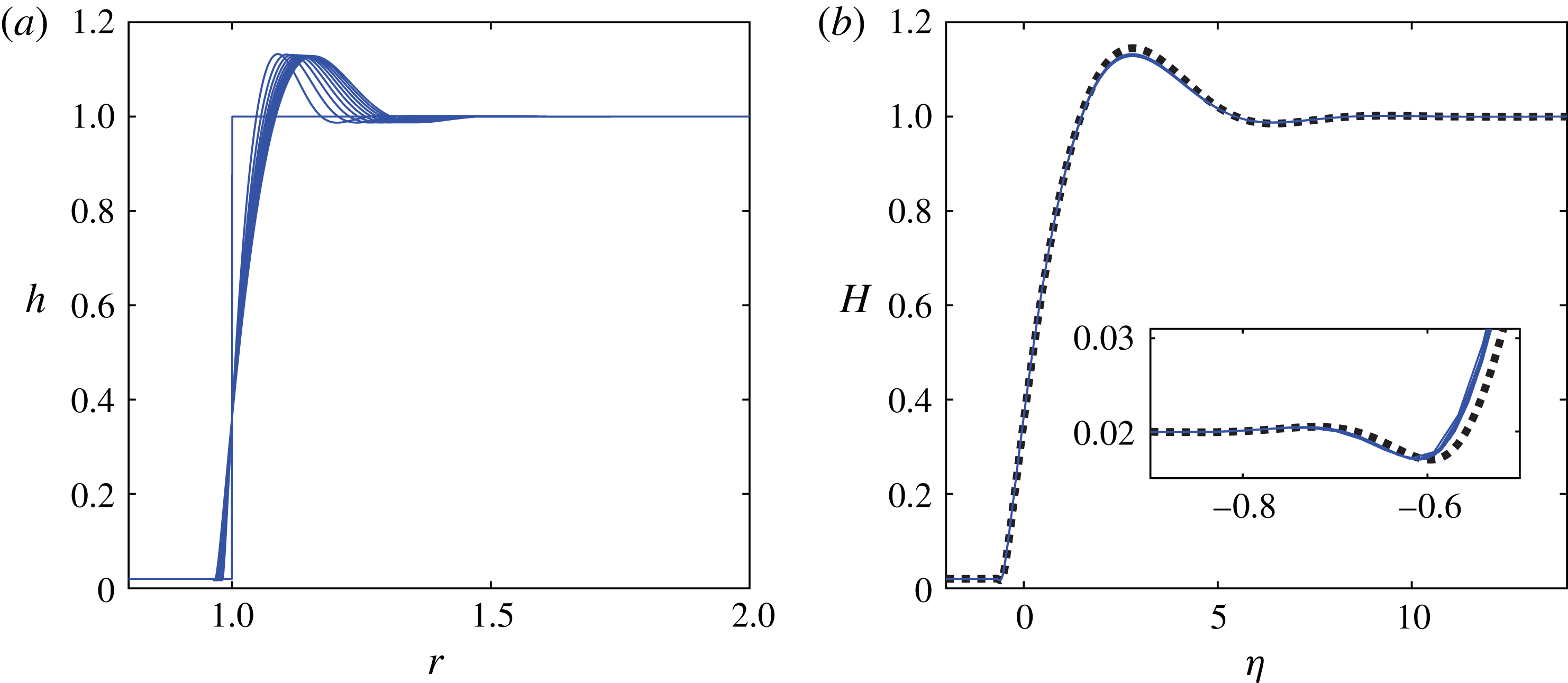
The main feature of the solutions depicted in figure 16 is the creation of capillary oscillations on both sides of the initial step. On the side of the thick film (
 $r>1$
) a large capillary ridge forms, which moves towards the outer boundary, while on the side of the prewetting film (
 $r<1$
) the small oscillations preceding the moving (apparent) contact line are reminiscent of those that exist in related problems (see e.g. Bertozzi et al.
Reference Bertozzi, Brenner, Dupont and Kadanoff1994; Eggers & Fontelos Reference Eggers and Fontelos2015), such as the linear problem that describes the dynamics of flexible filaments in a viscous fluid (Stone & Duprat Reference Stone and Duprat2016), and the Bretherton problem (Bretherton Reference Bretherton1961), in which a thin prewetting film connects to an advancing apparent contact line. We also note that, although the thin-film model equation is strictly speaking valid for small interfacial slopes and is expected to break down when interfacial slopes are large, experimental work appears to support the use of thin-film models to describe the relaxation process from step initial shapes (see e.g. Huppert & Woods Reference Huppert and Woods1995; McGraw et al.
Reference McGraw, Salez, Baumchen, Raphael and Dalnoki-Veress2012).
Appendix B. Far-field asymptotics
Here we analyse the asymptotic behaviour of the solutions of (2.10) for the special value
 $\unicode[STIX]{x1D6FD}=2/5$
in the far field (i.e. as
 $\unicode[STIX]{x1D709}\rightarrow \infty$
). First, we note that
 $f=\unicode[STIX]{x1D709}^{1/2}$
is an exact solution, as mentioned in § 2.2. Thus, we impose the far-field behaviour in the form
 $$\begin{eqnarray}f(\unicode[STIX]{x1D709})=a_{1}\unicode[STIX]{x1D709}^{1/2}+\tilde{f}(\unicode[STIX]{x1D709})\quad \text{as}\;\unicode[STIX]{x1D709}\rightarrow \infty ,\end{eqnarray}$$
where
 $\tilde{f}(\unicode[STIX]{x1D709})\ll \unicode[STIX]{x1D709}^{1/2}$
.
For simplicity and without loss of generality, we impose
 $a_{1}=1$
. Then, we substitute (B 1) in (2.10) and obtain the following linearized equation:
 $$\begin{eqnarray}-\frac{1}{5}\tilde{f}+\frac{2}{5}\unicode[STIX]{x1D709}\frac{\text{d}\tilde{f}}{\text{d}\unicode[STIX]{x1D709}}+\frac{1}{\unicode[STIX]{x1D709}}\frac{\text{d}}{\text{d}\unicode[STIX]{x1D709}}\left(-\frac{9}{8}\unicode[STIX]{x1D709}^{-1/2}\tilde{f}+\unicode[STIX]{x1D709}^{5/2}\frac{\text{d}}{\text{d}\unicode[STIX]{x1D709}}\left[\frac{1}{\unicode[STIX]{x1D709}}\frac{\text{d}}{\text{d}\unicode[STIX]{x1D709}}\left(\unicode[STIX]{x1D709}\frac{\text{d}\tilde{f}}{\text{d}\unicode[STIX]{x1D709}}\right)\right]\right)=0,\end{eqnarray}$$
which can be simplified to the form
 $$\begin{eqnarray}\unicode[STIX]{x1D709}^{3/2}\frac{\text{d}^{4}\tilde{f}}{\text{d}\unicode[STIX]{x1D709}^{4}}+\frac{7}{2}\unicode[STIX]{x1D709}^{1/2}\frac{\text{d}^{3}\tilde{f}}{\text{d}\unicode[STIX]{x1D709}^{3}}+\frac{1}{2}\unicode[STIX]{x1D709}^{-1/2}\frac{\text{d}^{2}\tilde{f}}{\text{d}\unicode[STIX]{x1D709}^{2}}+\frac{2}{5}\unicode[STIX]{x1D709}\frac{\text{d}\tilde{f}}{\text{d}\unicode[STIX]{x1D709}}-\frac{1}{5}\tilde{f}=0.\end{eqnarray}$$
Next, we employ a WKB strategy, and make the following substitution:
 $$\begin{eqnarray}\tilde{f}=\text{e}^{-W}.\end{eqnarray}$$
Assuming that
 $W^{\prime \prime }\ll (W^{\prime })^{2}$
,
 $W^{\prime \prime \prime }\ll (W^{\prime })^{3}$
and
 $W^{\prime \prime \prime \prime }\ll (W^{\prime })^{4}$
, where
 $^{\prime }$
denotes
 $\text{d}/\text{d}\unicode[STIX]{x1D709}$
, equation (B 3) can be simplified to the equation
 $$\begin{eqnarray}\unicode[STIX]{x1D709}^{3/2}(W^{\prime })^{4}-{\textstyle \frac{7}{2}}\unicode[STIX]{x1D709}^{1/2}(W^{\prime })^{3}+{\textstyle \frac{1}{2}}\unicode[STIX]{x1D709}^{-1/2}(W^{\prime })^{2}-{\textstyle \frac{2}{5}}\unicode[STIX]{x1D709}W^{\prime }-{\textstyle \frac{1}{5}}=0.\end{eqnarray}$$
We further make the substitution
 $$\begin{eqnarray}W^{\prime }=\unicode[STIX]{x1D709}^{-1/6}V.\end{eqnarray}$$
Then, equation (B 5) can be rewritten as
 $$\begin{eqnarray}\unicode[STIX]{x1D709}^{5/6}V^{4}-{\textstyle \frac{7}{2}}V^{3}+{\textstyle \frac{1}{2}}\unicode[STIX]{x1D709}^{-5/6}V^{2}-{\textstyle \frac{2}{5}}\unicode[STIX]{x1D709}^{5/6}V-{\textstyle \frac{1}{5}}=0,\end{eqnarray}$$
and the leading-order balance is
 $$\begin{eqnarray}\unicode[STIX]{x1D709}^{5/6}V^{4}-{\textstyle \frac{2}{5}}\unicode[STIX]{x1D709}^{5/6}V=0,\end{eqnarray}$$
which provides three non-trivial solutions for
 $V$
:
 $$\begin{eqnarray}V=\left({\textstyle \frac{2}{5}}\right)^{1/3},\left({\textstyle \frac{2}{5}}\right)^{1/3}\text{e}^{\pm 2\unicode[STIX]{x03C0}\text{i}/3}.\end{eqnarray}$$
The two complex roots are neglected since they lead to
 $\tilde{f}(\unicode[STIX]{x1D709})$
being highly oscillatory and growing faster than any power-law behaviour. To compute the next-order contribution to
 $V$
, we write
 $$\begin{eqnarray}V=\left({\textstyle \frac{2}{5}}\right)^{1/3}+\tilde{V}(\unicode[STIX]{x1D709}),\end{eqnarray}$$
where
 $\tilde{V}\ll 1$
, and, substituting (B 10) in (B 7), can obtain
 $$\begin{eqnarray}\tilde{V}={\textstyle \frac{8}{5}}\unicode[STIX]{x1D709}^{-5/6}.\end{eqnarray}$$
Substituting (B 10) and (B 11) in (B 6), we can obtain the asymptotic expression in the far field for
 $W(\unicode[STIX]{x1D709})$
,
 $$\begin{eqnarray}W={\textstyle \frac{6}{5}}\left({\textstyle \frac{2}{5}}\right)^{1/3}\unicode[STIX]{x1D709}^{5/6}+{\textstyle \frac{8}{5}}\quad \text{ln}~\unicode[STIX]{x1D709}+O(1),\end{eqnarray}$$
and also the asymptotic expression for
 $\tilde{f}(\unicode[STIX]{x1D709})$
using (B 4) and for
 $f(\unicode[STIX]{x1D709})$
using (B 1) with
 $a_{1}=1$
:
 $$\begin{eqnarray}f(\unicode[STIX]{x1D709})\sim \unicode[STIX]{x1D709}^{1/2}+\tilde{a}_{2}\unicode[STIX]{x1D709}^{-8/5}\text{e}^{-(6/5)\left(2/5\right)^{1/3}\unicode[STIX]{x1D709}^{5/6}}\quad \text{as}\;\unicode[STIX]{x1D709}\rightarrow \infty ,\end{eqnarray}$$
where
 $\tilde{a}_{2}$
is a constant.
We recall that to obtain (B 13) we set
 $a_{1}=1$
in (B 1) for simplicity (but without loss of generality). In fact, due to the invariance of (2.10) for
 $\unicode[STIX]{x1D6FD}=2/5$
under the transformation
 $f\mapsto \unicode[STIX]{x1D706}f$
,
 $\unicode[STIX]{x1D709}\mapsto \unicode[STIX]{x1D706}^{3/4}\unicode[STIX]{x1D709}$
, where
 $\unicode[STIX]{x1D706}$
is a positive constant, we obtain the following more general asymptotic behaviour of
 $f(\unicode[STIX]{x1D709})$
as
 $\unicode[STIX]{x1D709}\rightarrow \infty$
:
 $$\begin{eqnarray}\unicode[STIX]{x1D706}f(\unicode[STIX]{x1D709})\sim \left(\unicode[STIX]{x1D706}^{3/4}\unicode[STIX]{x1D709}\right)^{1/2}+\tilde{a}_{2}\left(\unicode[STIX]{x1D706}^{3/4}\unicode[STIX]{x1D709}\right)^{-8/5}\text{e}^{-(6/5)\left(2/5\right)^{1/3}\left(\unicode[STIX]{x1D706}^{3/4}\unicode[STIX]{x1D709}\right)^{5/6}},\end{eqnarray}$$
which can be rearranged to the form
 $$\begin{eqnarray}f(\unicode[STIX]{x1D709})\sim a_{1}\unicode[STIX]{x1D709}^{1/2}+a_{2}\unicode[STIX]{x1D709}^{-8/5}\text{e}^{-(6/5)\left(2/5\right)^{1/3}a_{1}^{-1}\unicode[STIX]{x1D709}^{5/6}}\quad \text{as}\;\unicode[STIX]{x1D709}\rightarrow \infty ,\end{eqnarray}$$
where
 $a_{1}\equiv \unicode[STIX]{x1D706}^{-5/8}$
and
 $a_{2}\equiv \tilde{a}_{2}\unicode[STIX]{x1D706}^{-11/5}$
.
Appendix C. Near-field asymptotics
C.1 Asymptotics for touch-down at the origin
If
 $f\rightarrow 0$
as
 $\unicode[STIX]{x1D709}$
approaches the origin, then in general,
 $$\begin{eqnarray}f\sim {\textstyle \frac{3}{20}}(75\unicode[STIX]{x1D6FC}-100\unicode[STIX]{x1D6FD})\unicode[STIX]{x1D709}^{4/3},\end{eqnarray}$$
while if
 $\unicode[STIX]{x1D6FD}=2/5$
there is also the special behaviour
 $f\sim c\unicode[STIX]{x1D709}^{1/2}$
for any
 $c$
, as this is an exact solution over all
 $\unicode[STIX]{x1D709}$
.
C.2 Asymptotics for the blow-up solutions
Next, we analyse the asymptotic behaviour of solutions of (2.10) that blow up at the origin. We first assume the power-law form
 $f\sim b_{1}\unicode[STIX]{x1D709}^{\unicode[STIX]{x1D6FE}}$
with
 $\unicode[STIX]{x1D6FE}<0$
. Substituting this expression in (2.10), we obtain the leading-order behaviour of each term:
 $$\begin{eqnarray}\displaystyle \left.\begin{array}{@{}c@{}}\displaystyle -\frac{4\unicode[STIX]{x1D6FD}-1}{3}f+\unicode[STIX]{x1D6FD}\unicode[STIX]{x1D709}f^{\prime }\sim \left(-\frac{4\unicode[STIX]{x1D6FD}-1}{3}+\unicode[STIX]{x1D6FD}\unicode[STIX]{x1D6FE}\right)b_{1}\unicode[STIX]{x1D709}^{\unicode[STIX]{x1D6FE}},\\ \displaystyle \frac{1}{\unicode[STIX]{x1D709}}\left[\unicode[STIX]{x1D709}f^{3}\left(\frac{1}{\unicode[STIX]{x1D709}}(\unicode[STIX]{x1D709}f^{\prime })^{\prime }\right)^{\prime }\right]^{\prime }\sim \unicode[STIX]{x1D6FE}^{2}(\unicode[STIX]{x1D6FE}-2)b_{1}\unicode[STIX]{x1D709}^{4\unicode[STIX]{x1D6FE}-2}.\end{array}\right\} & & \displaystyle\end{eqnarray}$$
No balance is possible for negative
 $\unicode[STIX]{x1D6FE}$
, so
 $f$
does not behave as a simple power law.
We therefore assume a general power-law-logarithmic expansion of the form
 $$\begin{eqnarray}f\sim \mathop{\sum }_{j=1}^{\infty }b_{j}\unicode[STIX]{x1D709}^{\unicode[STIX]{x1D6FE}_{j}}(-\!\log \unicode[STIX]{x1D709})^{\unicode[STIX]{x1D6E5}_{j}},\end{eqnarray}$$
where
 $\unicode[STIX]{x1D6FE}_{1}\leqslant 0,\unicode[STIX]{x1D6E5}_{1}>0$
is required for blow-up. Substitution of (C 3) into the terms in (2.10) gives the leading-order behaviour
 $$\begin{eqnarray}\displaystyle & \displaystyle -\frac{1}{5}f+\frac{2}{5}\unicode[STIX]{x1D709}f^{\prime }\sim \left(-\frac{4\unicode[STIX]{x1D6FD}-1}{3}+\unicode[STIX]{x1D6FD}\unicode[STIX]{x1D6FE}_{1}\right)b_{1}\unicode[STIX]{x1D709}^{\unicode[STIX]{x1D6FE}_{1}}(-\!\log \unicode[STIX]{x1D709})^{\unicode[STIX]{x1D6E5}_{1}}, & \displaystyle\end{eqnarray}$$
 $$\begin{eqnarray}\displaystyle & \displaystyle \frac{1}{\unicode[STIX]{x1D709}}\left[\unicode[STIX]{x1D709}f^{3}\left(\frac{1}{\unicode[STIX]{x1D709}}(\unicode[STIX]{x1D709}f^{\prime })^{\prime }\right)^{\prime }\right]^{\prime }\sim \unicode[STIX]{x1D6FE}_{1}^{2}(\unicode[STIX]{x1D6FE}_{1}-2)(4\unicode[STIX]{x1D6FE}_{1}-2)b_{1}^{4}\unicode[STIX]{x1D709}^{4\unicode[STIX]{x1D6FE}_{1}-4}(-\!\log \unicode[STIX]{x1D709})^{4\unicode[STIX]{x1D6E5}_{1}},\quad \unicode[STIX]{x1D6FE}_{1}\neq 0. & \displaystyle\end{eqnarray}$$
The second term (C 5), resulting from the surface tension term in (2.10), is too singular to match with (C 4) with
 $\unicode[STIX]{x1D6FE}_{1}\neq 0$
, so we must have
 $\unicode[STIX]{x1D6FE}_{1}=0$
. Taking
 $\unicode[STIX]{x1D6FE}_{1}=0$
, the asymptotic behaviour is
 $$\begin{eqnarray}\frac{1}{\unicode[STIX]{x1D709}}\left[\unicode[STIX]{x1D709}f^{3}\left(\frac{1}{\unicode[STIX]{x1D709}}(\unicode[STIX]{x1D709}f^{\prime })^{\prime }\right)^{\prime }\right]^{\prime }\sim 4b_{1}^{4}\unicode[STIX]{x1D6E5}_{1}(\unicode[STIX]{x1D6E5}_{1}-1)\frac{(-\!\log \unicode[STIX]{x1D709})^{4\unicode[STIX]{x1D6E5}_{1}-2}}{\unicode[STIX]{x1D709}^{4}},\quad \unicode[STIX]{x1D6E5}_{1}\neq 0,1.\end{eqnarray}$$
Again, this is too singular to match with (C 4), so
 $\unicode[STIX]{x1D6E5}_{1}=1$
. The coefficient
 $b_{1}$
is arbitrary.
Continuing this process, we find that the exponents of the first three terms are determined in a similar manner:
 $(\unicode[STIX]{x1D6FE}_{2},\unicode[STIX]{x1D6E5}_{2})=(0,0)$
,
 $(\unicode[STIX]{x1D6FE}_{3},\unicode[STIX]{x1D6E5}_{3})=(2,0)$
,
 $(\unicode[STIX]{x1D6FE}_{4},\unicode[STIX]{x1D6E5}_{4})=(2,-2)$
, with
 $b_{2},b_{3},b_{4}$
arbitrary. The fifth term in (C 3) does not feature an arbitrary constant, as it must cancel out the
 $O(\unicode[STIX]{x1D709}^{-2}(-\!\log \unicode[STIX]{x1D709})^{-2})$
term introduced by the fourth term in (C 3), giving
 $b_{5}=-2b_{4}(b_{1}+b_{2})/b_{1}$
. The same holds for higher terms, with the first term matching with (C 4) occurring at
 $O(\unicode[STIX]{x1D709}^{4}(-\!\log \unicode[STIX]{x1D709})^{-2})$
. We thus obtain the following asymptotic expansion:
 $$\begin{eqnarray}f\sim b_{1}(-\log \unicode[STIX]{x1D709})+b_{2}+b_{3}\unicode[STIX]{x1D709}^{2}+b_{4}\frac{\unicode[STIX]{x1D709}^{2}}{(-\!\log \unicode[STIX]{x1D709})^{2}}+O\left(\frac{\unicode[STIX]{x1D709}^{2}}{(-\!\log \unicode[STIX]{x1D709})^{3}}\right),\end{eqnarray}$$
where
 $b_{1},b_{2},b_{3},b_{4}$
are parameters. As a special case it includes thick-film solutions when
 $b_{1}=b_{4}=0$
, in which case
 $f$
is analytic and the error term is
 $O(\unicode[STIX]{x1D709}^{4})$
.
C.3 Asymptotics near a touch-down point
In this section, we analyse the asymptotic behaviour of solutions of (2.10) near a touch-down point
 $\unicode[STIX]{x1D709}_{0}>0$
. The leading-order terms of (2.10) near
 $\unicode[STIX]{x1D709}_{0}$
are
 $$\begin{eqnarray}\unicode[STIX]{x1D6FD}\unicode[STIX]{x1D709}_{0}\frac{\text{d}f}{\text{d}\unicode[STIX]{x1D709}}+\frac{\text{d}}{\text{d}\unicode[STIX]{x1D709}}\left(f^{3}\frac{\text{d}^{3}f}{\text{d}\unicode[STIX]{x1D709}^{3}}\right)=0.\end{eqnarray}$$
Integrating (C 8) once provides
 $$\begin{eqnarray}\unicode[STIX]{x1D6FD}\unicode[STIX]{x1D709}_{0}f+f^{3}\frac{\text{d}^{3}f}{\text{d}\unicode[STIX]{x1D709}^{3}}=\unicode[STIX]{x1D716}.\end{eqnarray}$$
We assume the power-law form
 $f\sim c_{1}\left(\unicode[STIX]{x1D709}-\unicode[STIX]{x1D709}_{0}\right)^{\unicode[STIX]{x1D6E5}_{1}}+c_{2}(\unicode[STIX]{x1D709}-\unicode[STIX]{x1D709}_{0})^{\unicode[STIX]{x1D6E5}_{2}}+\ldots$
with
 $0<\unicode[STIX]{x1D6E5}_{1}<\unicode[STIX]{x1D6E5}_{2},\ldots$
, and
 $c_{1}>0$
. Then, on substitution into (C 9) we obtain
 $\unicode[STIX]{x1D6E5}=3/4$
,
 $c_{1}=(64\unicode[STIX]{x1D716}/15)^{1/4}$
(or, equivalently,
 $\unicode[STIX]{x1D716}=15c_{1}^{4}/64$
),
 $\unicode[STIX]{x1D6E5}_{2}=3/2$
and
 $c_{2}=-(64\unicode[STIX]{x1D6FD}\unicode[STIX]{x1D709}_{0})/(21c_{1}^{2})$
, thus:
 $$\begin{eqnarray}f\sim (64\unicode[STIX]{x1D716}/15)^{1/4}\left(\unicode[STIX]{x1D709}-\unicode[STIX]{x1D709}_{0}\right)^{3/4}-\frac{8\sqrt{15}\unicode[STIX]{x1D6FD}\unicode[STIX]{x1D709}_{0}}{21\sqrt{\unicode[STIX]{x1D716}}}(\unicode[STIX]{x1D709}-\unicode[STIX]{x1D709}_{0})^{3/2}.\end{eqnarray}$$
We note that such generic touch-down behaviour occurs only for
 $\unicode[STIX]{x1D716}>0$
. When
 $\unicode[STIX]{x1D716}<0$
, there is no real solution for
 $c_{1}$
, and we do not have a power-law behaviour touching the
 $\unicode[STIX]{x1D709}$
-axis from above as
 $\unicode[STIX]{x1D709}\rightarrow \unicode[STIX]{x1D709}_{0}^{+}$
.
Generic touch-down corresponds to
 $\unicode[STIX]{x1D716}>0$
. In the limit
 $\unicode[STIX]{x1D716}\rightarrow 0^{+}$
(or, equivalently,
 $c_{1}\rightarrow 0$
) the generic touch-down (C 10) becomes singular, as the coefficient of the second term blows up. In fact, Duffy & Wilson (Reference Duffy and Wilson1996) have shown that for solutions of (C 9) with
 $\unicode[STIX]{x1D716}=0$
, there are no solutions touching down the
 $\unicode[STIX]{x1D709}$
-axis from above as
 $\unicode[STIX]{x1D709}\rightarrow \unicode[STIX]{x1D709}_{0}^{+}$
. In this case, the behaviour of
 $f$
near
 $\unicode[STIX]{x1D709}=\unicode[STIX]{x1D709}_{0}$
is (assuming
 $\unicode[STIX]{x1D709}>\unicode[STIX]{x1D709}_{0}$
)
 $$\begin{eqnarray}f\sim -\left(3\unicode[STIX]{x1D6FD}\unicode[STIX]{x1D709}_{0}\right)^{1/3}(\unicode[STIX]{x1D709}-\unicode[STIX]{x1D709}_{0})[-\!\log (\unicode[STIX]{x1D709}-\unicode[STIX]{x1D709}_{0})]^{1/3}.\end{eqnarray}$$
This cannot approach the touch-down point from above, so, as with the case where
 $\unicode[STIX]{x1D716}<0$
, this touch-down behaviour does not pertain to the similarity solutions we consider.
Finally, as well as the touch-down solutions, equation (C 9) admits solutions that remain strictly positive. These solutions are also relevant to the travelling wave or ‘quasi-steady’ moving contact line between a fluid body and a much thinner prewetting film, originally derived by Landau & Levich (Reference Landau and Levich1942) (see also Myers Reference Myers1998). The
 $\unicode[STIX]{x1D709}\gg \unicode[STIX]{x1D709}_{0}$
behaviour of such solutions is either quadratic [
 $f\propto (\unicode[STIX]{x1D709}-\unicode[STIX]{x1D709}_{0})^{2}$
] or almost linear [
 $f\propto (\unicode[STIX]{x1D709}-\unicode[STIX]{x1D709}_{0})\log ^{1/3}(\unicode[STIX]{x1D709}-\unicode[STIX]{x1D709}_{0})$
] (Bender & Orszag Reference Bender and Orszag1978; Eggers Reference Eggers2004). Our numerical results have indicated that the solution to (2.10) with this behaviour matches to the latter behaviour and is unique for a given
 $\unicode[STIX]{x1D6FD}$
. This solution is approached as
 $c_{1}$
, say, is reduced to near zero, as long as
 $\unicode[STIX]{x1D6FD}$
is greater than
 $2/5$
. The full similarity solution (2.10) does not support the existence of a prewetting film (as constant
 $f=f_{pw}$
is not a solution to (2.10)), so the similarity solution can only be assumed to hold in some region near the contact line.
Appendix D. Self-similar solutions using numerical continuation
The self-similar solutions to the ODE (2.10) were computed using shooting in § 2. Another method of computation is to solve the governing equation as a boundary-value problem on a suitably large domain. Here we compute the solutions to generic touch-down using such a method, implemented in the numerical continuation package AUTO-07p (Doedel et al.
Reference Doedel, Champneys, Dercole, Fairgrieve, Kuznetsov, Oldeman, Paffenroth, Sandstede, Wang and Zhang2007). Numerical continuation is a particularly useful and powerful method to use, as it allows us to systematically and efficiently compute the one-parameter family of solutions (parametrized, say, by
 $\unicode[STIX]{x1D709}_{0}$
) for each exponent
 $\unicode[STIX]{x1D6FD}$
. We note that numerical continuation techniques have also been used for computation of self-similar solutions in a related problem of a thin-film rupture on a solid substrate: see Tseluiko, Baxter & Thiele (Reference Tseluiko, Baxter and Thiele2013), Dallaston et al. (Reference Dallaston, Tseluiko, Zheng, Fontelos and Kalliadasis2017).
Firstly, we compute solutions with a generic touch-down behaviour at
 $\unicode[STIX]{x1D709}_{0}$
. Since we expect
 $f\sim c_{1}(\unicode[STIX]{x1D709}-\unicode[STIX]{x1D709}_{0})^{3/4}$
, we perform the change of variables
 $$\begin{eqnarray}\unicode[STIX]{x1D709}=\unicode[STIX]{x1D709}_{0}+z^{4},\quad f=z^{3}g(z),\end{eqnarray}$$
which removes the singularity at
 $\unicode[STIX]{x1D709}=\unicode[STIX]{x1D709}_{0}$
, so that
 $g$
is smooth in
 $z$
. Now, we define state variables
 $$\begin{eqnarray}U_{1}=g,\quad U_{2}=\frac{\unicode[STIX]{x1D709}_{0}+z^{4}}{4}(zg^{\prime }+3g),\quad U_{3}=\frac{zU_{2}^{\prime }-U_{2}}{4(\unicode[STIX]{x1D709}_{0}+z^{4})},\quad U_{4}=\frac{(\unicode[STIX]{x1D709}_{0}+z^{4})g^{3}}{4}(zU_{3}^{\prime }-5U_{3}),\end{eqnarray}$$
(where
 $^{\prime }$
represents differentiation with respect to
 $z$
), from which we obtain a system of four first-order ODEs:
 $$\begin{eqnarray}\displaystyle U_{1}^{\prime } & = & \displaystyle \frac{1}{z}\left[\frac{4}{\unicode[STIX]{x1D709}_{0}+z^{4}}U_{2}-3g\right],\end{eqnarray}$$
 $$\begin{eqnarray}\displaystyle U_{2}^{\prime } & = & \displaystyle \frac{1}{z}\left[4(\unicode[STIX]{x1D709}_{0}+z^{4})U_{3}+U_{2}\right],\end{eqnarray}$$
 $$\begin{eqnarray}\displaystyle U_{3}^{\prime } & = & \displaystyle \frac{1}{z}\left[\frac{4}{(\unicode[STIX]{x1D709}_{0}+z^{4})U_{1}^{3}}U_{4}+5U_{3}\right],\end{eqnarray}$$
 $$\begin{eqnarray}\displaystyle U_{4}^{\prime } & = & \displaystyle 4\unicode[STIX]{x1D6FC}(\unicode[STIX]{x1D709}_{0}+z^{4})z^{6}U_{1}-4\unicode[STIX]{x1D6FD}(\unicode[STIX]{x1D709}_{0}+z^{4})z^{2}U_{2}.\end{eqnarray}$$
The last of these comes from equation (2.10).
The boundary conditions follow from the analysis of the far-field and touch-down behaviour discussed in appendices B and (C.3), respectively. In particular, we found that for the far-field behaviour there are two growing modes as
 $\unicode[STIX]{x1D709}\rightarrow \infty$
(or, equivalently, as
 $z\rightarrow \infty$
). To eliminate these modes, it is appropriate to impose two boundary conditions that are consistent with the far-field behaviour. We can impose, for instance, the conditions
 $$\begin{eqnarray}U_{2}\sim \frac{\unicode[STIX]{x1D6FC}}{\unicode[STIX]{x1D6FD}}z^{4}U_{1},\quad U_{3}\sim \frac{\unicode[STIX]{x1D6FC}^{2}}{\unicode[STIX]{x1D6FD}^{2}}U_{1}\quad \text{as}\;z\rightarrow \infty .\end{eqnarray}$$
In practice these conditions are imposed at
 $z=L$
for sufficiently large
 $L$
.
The generic touch-down behaviour has one growing mode as
 $\unicode[STIX]{x1D709}\rightarrow \unicode[STIX]{x1D709}_{0}^{+}$
(or, equivalently, as
 $z\rightarrow 0$
). To eliminate this mode, it is appropriate to impose one boundary condition, e.g.
 $$\begin{eqnarray}U_{2}=\frac{3\unicode[STIX]{x1D709}_{0}U_{1}}{4}\quad \text{at}\;z=0,\end{eqnarray}$$
which follows from substituting
 $z=0$
in the definition of
 $U_{2}$
in (D 2).
In addition, to eliminate scale invariance of the solutions, we need to impose one more condition. We can, for example, impose
 $$\begin{eqnarray}U_{1}\sim a_{1}z^{4\unicode[STIX]{x1D6FC}/\unicode[STIX]{x1D6FD}-3},\end{eqnarray}$$
with a given value of
 $a_{1}$
. In our calculations, we use
 $a_{1}=1$
for direct comparison with figure 3.
This completes the formulation of the boundary-value problem. One of the parameters can be used as the continuation parameter to obtain families of solutions. For example, rather than varying a far-field parameter (as is necessary in shooting), we may instead vary
 $\unicode[STIX]{x1D709}_{0}$
(for fixed values of
 $\unicode[STIX]{x1D6FD}$
and
 $L$
). To track how coefficient
 $c_{1}$
varies along a family of solutions, we can add
 $c_{1}$
as an additional parameter in the formulation of the boundary-value problem and impose one more boundary condition, e.g.
 $$\begin{eqnarray}U_{1}=c_{1}.\end{eqnarray}$$
We plot the results of continuation in figure 17 in the
 $(\unicode[STIX]{x1D709}_{0},c_{1})$
plane for various values of
 $\unicode[STIX]{x1D6FD}$
. We used
 $L=16$
in the computations. We note that for each
 $\unicode[STIX]{x1D6FD}>0$
, an apparent critical value of
 $\unicode[STIX]{x1D709}_{0}$
is approached as
 $c_{1}\rightarrow 0$
, until a sharp turn in the
 $(\unicode[STIX]{x1D709}_{0},c_{1})$
curve that corresponds to the growth of a ‘foot’ with a well-defined thickness
 $f_{pw}$
. The apparent contact-line location remains fixed as
 $\unicode[STIX]{x1D709}_{0}\rightarrow 0$
. We may thus build up a
 $f_{pw}$
versus
 $\unicode[STIX]{x1D6FD}$
curve, that matches with the results from shooting in figure 4. As
 $\unicode[STIX]{x1D6FD}$
gets close to 0.4, the prewetting thickness becomes too small to resolve.
(a) Families of self-similar solutions to (2.10) in the
 $(\unicode[STIX]{x1D709}_{0},c_{1})$
-plane computed using numerical continuation, for various values of
 $\unicode[STIX]{x1D6FD}$
. As
 $c_{1}$
is decreased, the profiles tend to a non-generic profile, shown in (b), with a foot of width
 $f_{pw}(\unicode[STIX]{x1D6FD})$
. (c–e) the region near the apparent contact line for (c)
 $\unicode[STIX]{x1D6FD}=0.5$
, (d)
 $\unicode[STIX]{x1D6FD}=0.48$
and (e)
 $\unicode[STIX]{x1D6FD}=0.46$
, showing the development of the foot as
 $c_{1}$
is decreased.
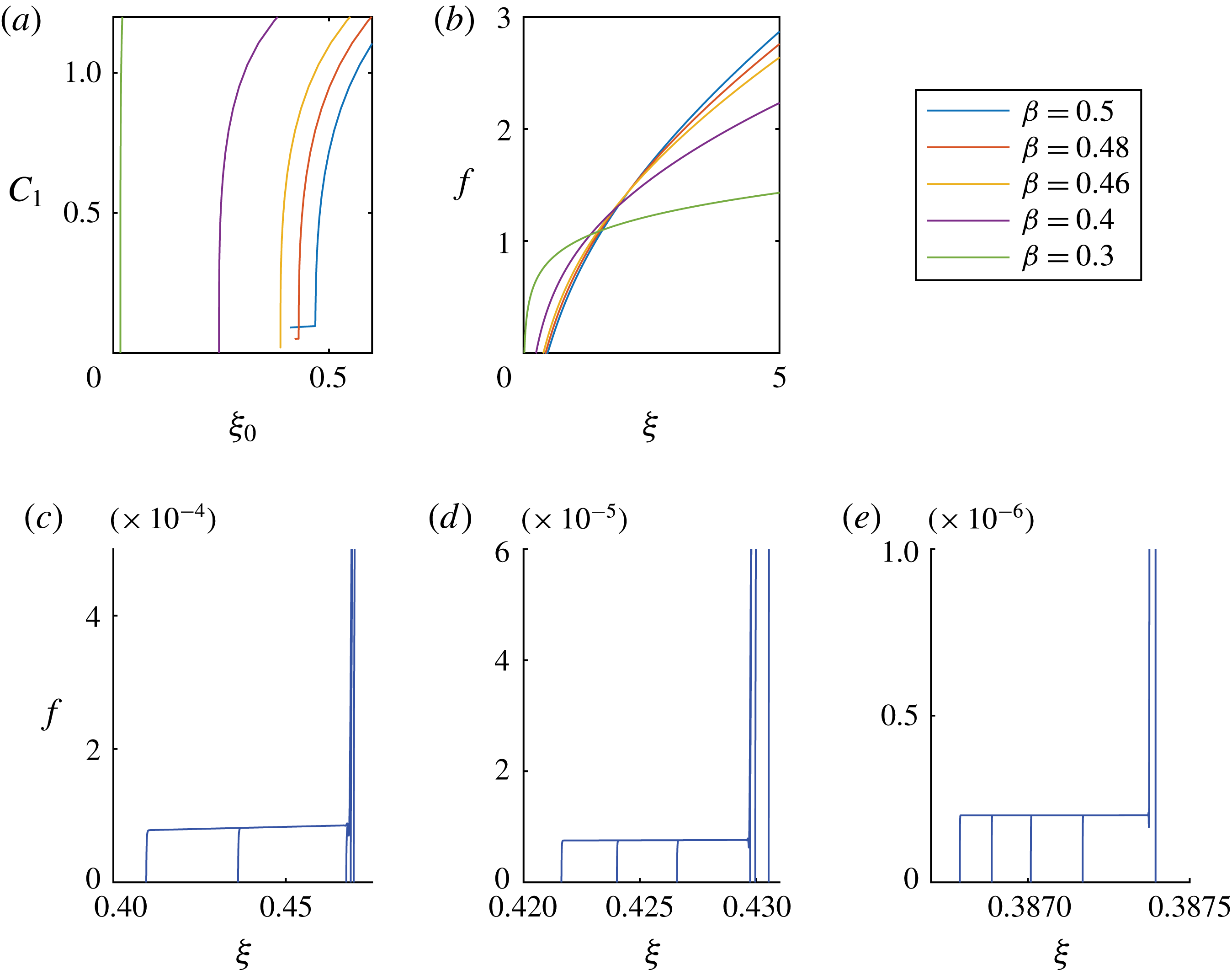
Appendix E. Numerical scheme
We use a finite-difference scheme to solve the PDE (2.5), subject to appropriate boundary conditions (2.7) and initial condition (2.6) on the domain
 $[0,10]$
. We first rewrite (2.5) as
 $$\begin{eqnarray}\frac{\unicode[STIX]{x2202}h}{\unicode[STIX]{x2202}t}+\frac{1}{r}\frac{\unicode[STIX]{x2202}}{\unicode[STIX]{x2202}r}\left(rhv\right)=0,\end{eqnarray}$$
where
 $$\begin{eqnarray}v\equiv h^{2}\frac{\unicode[STIX]{x2202}\unicode[STIX]{x1D705}}{\unicode[STIX]{x2202}r},\quad \text{and}\quad \unicode[STIX]{x1D705}\equiv \frac{1}{r}\frac{\unicode[STIX]{x2202}}{\unicode[STIX]{x2202}r}\left(r\frac{\unicode[STIX]{x2202}h}{\unicode[STIX]{x2202}r}\right).\end{eqnarray}$$
Equation (E 1) can be rearranged in the form
 $$\begin{eqnarray}\frac{\unicode[STIX]{x2202}(rh)}{\unicode[STIX]{x2202}t}+v\frac{\unicode[STIX]{x2202}(rh)}{\unicode[STIX]{x2202}r}+rh\frac{\unicode[STIX]{x2202}v}{\unicode[STIX]{x2202}r}=0,\end{eqnarray}$$
and we note that the first two terms represent the convection of
 $rh$
with velocity
 $v$
.
In the healing process, we expect a front advancing towards the origin, and we impose an upwind scheme to discretize the
 $r$
derivative of
 $rh$
. Hence, if we discretize
 $h$
at time
 $t$
by a set of values
 $\left\{h_{i}^{t}\right\}_{i=1}^{N}$
at the nodes
 $\left\{r_{i}\right\}_{i=1}^{N}$
, we obtain the discretized equation
 $$\begin{eqnarray}\frac{h_{i}^{t+\unicode[STIX]{x0394}t}-h_{i}^{t}}{\unicode[STIX]{x0394}t}=-\frac{v_{i}^{t}}{r_{i}}\frac{r_{i+1}h_{i+1}^{t}-r_{i}h_{i}^{t}}{r_{i+1}-r_{i}}-h_{i}^{t}\frac{v_{i+1/2}^{t}-v_{i-1/2}^{t}}{(r_{i+1}-r_{i-1})/2},\end{eqnarray}$$
where
 $$\begin{eqnarray}\displaystyle v_{i}^{t} & = & \displaystyle \left(h_{i}^{t}\right)^{2}\frac{\unicode[STIX]{x1D705}_{i+1}^{t}-\unicode[STIX]{x1D705}_{i-1}^{t}}{r_{i+1}-r_{i-1}},\end{eqnarray}$$
 $$\begin{eqnarray}\displaystyle v_{i+\frac{1}{2}}^{t} & = & \displaystyle \left(\frac{h_{i+1}^{t}+h_{i}^{t}}{2}\right)^{2}\frac{\unicode[STIX]{x1D705}_{i+1}^{t}-\unicode[STIX]{x1D705}_{i}^{t}}{r_{i+1}-r_{i}},\end{eqnarray}$$
 $$\begin{eqnarray}\displaystyle \unicode[STIX]{x1D705}_{i}^{t} & = & \displaystyle \frac{2}{r_{i+1}-r_{i-1}}\left(\frac{h_{i+1}^{t}-h_{i}^{t}}{r_{i+1}-r_{i}}-\frac{h_{i}^{t}-h_{i-1}^{t}}{r_{i}-r_{i-1}}\right)+\frac{1}{r_{i}}\frac{h_{i+1}^{t}-h_{i-1}^{t}}{r_{i+1}-r_{i-1}}.\end{eqnarray}$$
 $\unicode[STIX]{x1D705}_{i}^{t}$
is approximated using the central difference of
 $h_{i}^{t}$
. In order to resolve the structure of the profiles near the apparent contact line, the code is adaptive and introduces finer meshes in the regions where more nodes are needed. For example, the grid size is of
 $O(10^{-5})$
to
 $O(10^{-7})$
close to the centre of the hole, and the time step starts from
 $10^{-18}$
, for example, and gradually increases as time progresses. We performed convergence tests to verify that the results are insensitive to further mesh refinements.



