I. INTRODUCTION
It is well known that the famous Hall–Petch (H–P) equation can be generally used for modeling the dependence of the yield stress on the grain size of traditional polycrystalline materials. Over the past decade, however, it has been documented that as the grain size (d) is reduced to the nanometer regime, an inverse H–P behavior is observed. In other words, there is a critical nanograin size (d cr) where a “transition” occurs from hardening (d > d cr) to softening (d < d cr) behavior. There exist numerous experimental studies that document this hardening-to-softening behavior,Reference Sanders, Eastman and Weertman1–Reference Zhao, Li and Jiang8 and they all attribute it to the change in deformation mechanisms below a critical grain size due to grain boundary (GB) effects. Recently, further experiments have shown that such softening is also observed for nanotwinned Cu when the twin thickness is below 15 nm.Reference Lu, Chen, Huang and Lu9
Two main theoretical approaches have been followed in trying to interpret this “anomalous” H–P behavior for nanomaterials. One is based on dislocation mechanisms and associated changes as the grain size crosses over from the microcrystalline to the nanocrystalline regime. The other approach is based on geometry and the rule of mixtures by viewing the polycrystal as a superposition of “bulk” and “GB” material. Relevant references for both approaches can be found in Refs. Reference Meyers, Mishra and Benson10–Reference Saada, Dirras, Hirth and Kubin12 and references therein, as well as in the initial articlesReference Carsley, Ning, Milligan, Hackney and Aifantis13, Reference Konstantinidis and Aifantis14 where some background ideas related to this article are also used.
A third most recent approach has also been introduced that combines the aforementioned two as follows: (i) an interface energy term is introduced which depends on dislocation mechanisms at the interface and allows the interface to follow its own yield behavior and (ii) a boundary layer is considered which yields along with the GB while the grain interior (GI) remains elastic.Reference Aifantis and Konstantinidis15, Reference Aifantis and Konstantinidis16 This third approach, therefore, is a compromise of the first two since: (i) it distinguishes between “bulk” and “GB” behavior, by allowing the GB to follow its own plastic behavior through the introduction of an interface energy term and (ii) it accounts for a variety of underlying dislocation mechanisms by allowing for the development of strain gradients across the grain–GB interface.
Although the aforementioned underlying physical mechanisms of deformation are consistent with what occurs at the nanoscale, the theoretical approachReference Aifantis and Konstantinidis15, Reference Aifantis and Konstantinidis16 was based on a gradient plasticity model with an interface energy term that was developed for considering interfaces at the micronscale,Reference Aifantis and Willis17 which allow for dislocation pileups.
A limitation, hence, in applying the interface gradient plasticity worksReference Aifantis and Konstantinidis15, Reference Aifantis and Konstantinidis16 at the nanoscale, is that the GB was treated as a surface, rather than allowing it to have a finite thickness, which is the case for nanocrystals; furthermore, the interface energy was introduced phenomenologically, rather than being related to known material parameters. In this study, therefore, grain boundaries are allowed to have a finite width and by employing a different gradient plasticity framework, it is possible to obtain the local strain distribution in a nanocrystal. Particularly, the GB is allowed to act as a “strengthener” in the microcrystalline regime and as a “softener” in the nanocrystalline one, providing a unified simple analytical expression that can capture both the “normal” and “abnormal” H–P relation. The underlying idea is that the “bulk” and the “GB” spaces interchange their role to accommodate deformation as the grain size crosses over from the microcrystalline to the nanocrystalline regime. As the scale transitions to nanodimensions, the “bulk” becomes incapable of supporting dislocation nucleation and motion due to its small volume constrained by the relatively thick GB space (and adjacent layers), where most of the dislocation activity occurs, resulting in overall macroscopic plastic deformation.
In the sequel, it will be shown that allowing for this “GB” versus “grain” distinction the mechanical response of nanocrystals below a critical grain size can be captured. Furthermore, by directly relating the present gradient plasticity formulation to that used previouslyReference Aifantis and Konstantinidis15, Reference Aifantis and Konstantinidis16 allows for the interface energy to be defined as a function of the GB and GI material properties such as the yield stress. The theoretical model will be shown to be in precise agreement with both experimentalReference Sanders, Eastman and Weertman1–Reference Zhao, Li and Jiang8 and simulationReference Schiotz, Vegge, Di Tolla and Jacobsen18 data for nanomaterials.
It should be noted that in addition to the aforementioned three approaches, other individual models have also been developed to capture the inverse H–P relationship and resulted in the following conclusions: (i) impurity segregation at grain boundaries decreases as the scale decreases, resulting hence in softer boundaries and a softer overall response for nanomaterials below a certain grain size,Reference Li19 (ii) the nonequilibrium structure of nanosized grains results in softening,Reference Armstrong, Conrad, Nabarro, Ovid'ko, Pande, Krishnamoorti, Lavernia and Skandan20 and (iii) the melting temperature decrease of nanomaterials contributes to their hardness decrease.Reference Zhao, Li and Jiang8
II. CAPTURING THE INVERSE H–P RELATIONSHIP
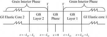
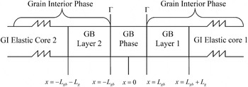
As mentioned in the introduction, gradient plasticity has been able to capture to some extent the inverse H–P behavior by allowing for an interface energy term. In this study, an alternative, more physically based model, will be presented that allows explicit consideration of grain boundaries in nanomaterials. In contrast to earlier papers,Reference Aifantis and Konstantinidis15, Reference Aifantis and Konstantinidis16 therefore, it is assumed here that the GB does not act as a surface of discontinuity for the plastic strain gradient and its conjugate third-order stress. Instead, it has a finite width δ = 2L gb and acts as a separate phase constrained by the two adjacent grains. Early experimental evidenceReference Ke, Hackney, Milligan and Aifantis21 has shown that below a critical grain size, deformation occurs through grain rotation and no dislocations form in the purely elastic grains. The GB, hence, in the present framework is assumed to be soft and prone to deformation through rotation/sliding, whereas the GI is purely elastic. In Ref. Reference Ovid'ko and Sheinerman22, it was theoretically described that during GB sliding, defects such as GB dislocations and dipoles of wedge disclinations are produced. Such defects are not constrained only into the GB phase, but diffuse to a limited extent into the grain phase, forming therefore a plastic GI–GB layer adjacent to the GB, while the remaining GI core remains purely elastic. The boundary layers, therefore, with thickness L g, allow for the transition from the ductile GB to the rigid grain core and are considered in the unit cell model of Fig. 1.
Unit cell model with grain boundary (GB) phase, grain interior (GI) phase comprised of GI–GB layers, and elastic GI cores.
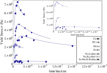
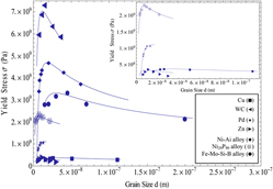
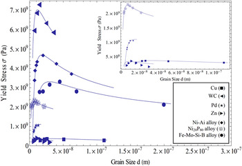
Fitting of experimental data to theory.
Before proceeding with listing the basic equations of the gradient plasticity theory used and its application to the unit cell configuration of Fig. 1, it is remarked that the key physical assumptions of the present model have also been used, in a different context and theoretical framework, by other prominent researchers in the past for deformation at the nanoscale. For example, previous theoretical frameworksReference Kim, Estrin and Bush23, Reference Kim, Estrin and Bush24 also assume GB softening to occur due to the underlying mechanism of Coble creep; further information on creep in nanomaterials can be found in Ref. Reference Armstrong, Buschow, Robert, Merton, Bernard, Edward, Subhash and Patrick25 and references therein. GB layers similar to that in Fig. 1 have also been successfully considered,Reference Fu, Benson and Meyers26, Reference Meyers and Ashworth27 while dislocation-based modelsReference Gutkin, Ovid’ko and Skiba28–Reference Padmanabhan and Gleiter30 consider that plastic flow occurs predominantly in the GB space network while the GI core remains elastic.
The basic structure of the gradient plasticity theory to be used is summarized below.
A. Gradient plasticity framework
In the strain gradient plasticity framework, both the displacement and plastic strain are the independent kinematic variables.Reference Aifantis and Ngan31 The uniqueness of the solution emerges by finding suitable displacement and plastic strain fields  that minimize the energy functional for the domain Ω under consideration:

where U is the elastoplastic potential energy density and depends on the total strain ε ij, the plastic strain  , and the plastic strain gradient
 , as
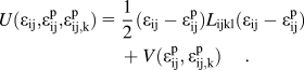
The quantity V is the gradient dependent plastic potential, and in the case of classical plasticity, it would not depend on  . The conjugate variables associated with
 are

Performing the principal of virtual work and applying the divergence theorem, the governing equilibrium relations in the plastically deformed volume are:

If the displacement is prescribed, the boundary conditions at the external surface are

And if one assumes the presence of internal boundaries within the domain Ω, the stress and higher-order stress would be continuous across them as the variational principle gives

where the brackets [f] denote the difference, f 1−f 2, of the enclosed quantity across the interface (the interface normal direction points from “side 2” to “side 1”). Hence, the stress, σ ij, and higher-order stress, τ ijk, are continuous across the boundaries where the GB phase meets with the boundary layer.
When a separate interface energy term,  , is assigned to grain boundaries, which are collectively denoted as Γ, the energy functional reads17

By carrying out the principle of virtual work, the same equilibrium and boundary conditions are obtained as before [Eqs. (4) and (5)], but now an interface condition is obtained as

B. Capturing the dependence of grain size on the yield stress
To proceed with analyzing the mechanical response of the one-dimensional configuration of Fig. 1, the plastic potential V must be defined. Since deformation at the nanoscale is not dominated by dislocation motion, strain hardening is not an expected deformation mechanism; instead deformation is taken to be perfectly plasticReference Carsley, Ning, Milligan, Hackney and Aifantis13 and, therefore, the plastic potential in the GB phase, and the adjacent to it GB layers, is taken to depend on the plastic strain gradient so as to allow for perfect plasticity after yieldingReference Aifantis and Willis17
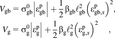
where (β gb, β g) and (ℓgb, ℓg) denote hardening moduli and internal lengths, respectively, while  and
 are the yield stresses and plastic strains of the GB and GB layer respectively; since the GB layer is part of the grain,
 is equal to yield stress of the grain. Inserting Eq. (8) in Eq. (4) and solving the resulting differential equation gives
 , (i = gb, g), where
 is the applied stress. The constants of integration Ai and Bi are obtained from the continuity conditions
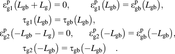
Finally, on setting the plastic strain gradient equal to zero at the interface of the GB layer with the elastic core of the GI, i.e.,  gives

It is interesting to note that Eq. (10) is essentially a statement of the rule of mixtures. On assuming that  , i.e., that the GB phase is softer than the GB layer, Eq. (10) suggests that the thickness of the GB layer increases as the applied stress
 increases.
Another interesting observation is to compute the difference τ(L gb)−τ(−L gb). According to Eq. (7) of the approach in Ref. Reference Aifantis and Willis17, the jump of τ across the GB equals the derivative of the interface energy parameter  . By letting ϕ(ε p) = γ gbε p, as in Refs.Reference Aifantis and Konstantinidis15 and Reference Aifantis and Konstantinidis16, it is found that
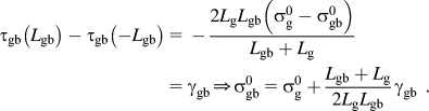
Equation (11) illustrates how the interface energy modelReference Aifantis and Willis17 can be related to the present multiphase model, which by allowing for grain boundaries to have a finite thickness, it derives a microscopic expression for the interface energy parameter γ gb. It should be noted that, according to Eq. (11), γ gb is positive as the grain boundaries inhibit plastic flow ( ), whereas at the nano regime, γ gb is negative as the grain boundaries become the carriers of plastic deformation and are softer than the GI (
 ).
Upon insertion of Eq. (11) into Eq. (10), we obtain
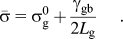
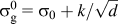
Since  is the yield stress of the grain, it can be allowed to follow the standard H–P relation, i.e.,
 and allowing the boundary layer thickness to be a fraction of the grain size d, i.e., Lg = ad with 0 < a < 1, Eq. (12) yields
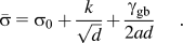
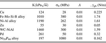
Equation (13) gives the stress of the unit cell depicted in Fig. 1 upon yielding of the GB and boundary layers; it, therefore, corresponds to the yield stress of the nanocrystal, and it is used to fit experimental data obtained for seven different nanocrystalline materials, which exhibit both normal and abnormal H–P behavior. In particular, such experimental data exist for Cu,Reference Sanders, Eastman and Weertman1 Fe-Mo-Si-B alloy,Reference Liu, Hu and Ding2 Ni-Al alloy,Reference Volpp, Göring, Kuschke and Arzt3 Zn,Reference Narayan, Venkatesan and Kvit4 WC-NiAl,Reference Venkatesan, Kvit, Wei, Narayan, Farkas, Kung, Mayo, Van Swygenhoven and Weertman5 Pd,Reference Chokshi, Rosen, Karch and Gleiter6, Reference Zhao, Li and Jiang8 and Ni20P80 alloy.Reference Palumbo, Erb and Aust7, Reference Zhao, Li and Jiang8 Although the fabrication methods for each nanocrystal differ, in all casesReference Sanders, Eastman and Weertman1–Reference Zhao, Li and Jiang8 their hardness was reported, and according to Tabor’s rule (hardness/3=σ 0),Reference Tabor32 it was converted into the yield stress so as to directly fit Eq. (13) to these data. The corresponding values of the parameters are given in Table I. A similar expression to that in Eq. (12) was obtained by the interface gradient plasticity model,Reference Aifantis and Konstantinidis15, Reference Aifantis and Konstantinidis16 but the underlying physical mechanisms were not elaborated as they are here.
Values of the parameters used to generate the fits in Fig. 2.
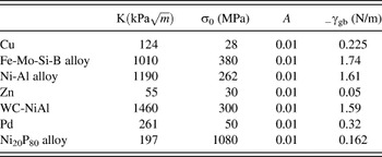
It should be noted that the values for the parameters in Table I cannot be compared with previous experimental data, since all existing data in the literature are for bulk or single crystal materials, not for nanocrystalline as in the present case.
Furthermore, it is noted that the critical grain size d c where the transition from the “normal” to the “abnormal” H–P behavior occurs can be determined from Eq. (13) by setting  , giving

Equation (14) can be thought of as the micro-to-nano scale transition criterion as it defines that the critical grain size at which material behavior “switches” from micron to nano can be directly computed if the GB energy (γ gb), the fraction of the GB thickness that yields (a), and the H–P slope (k) are known. Furthermore, inserting Eq. (14) in Eq. (13) provides the peak strength observed in crystalline materials. Although similar analytical expressions that can predict this transition do not exist, it was proposed in Ref. Reference Argon and Yip33 that the peak strength of nanomaterials is reached when the strain rate contribution from the GB shear is equal to the alternative contribution from dislocation plasticity inside the grain.
III. PREDICTING SIZE EFFECTS IN THE FLOW STRESS WHEN d < d c
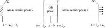
Having successfully interpreted the softening that occurs in the yield stress of nanocrystals as the grain size decreases, it is of interest to try and model the softening that takes place in the flow stress of such materials. Atomistic simulationsReference Schiotz, Vegge, Di Tolla and Jacobsen18 have shown that decreasing the grain size of nanocrystalline Cu below a critical value results in a softening in the flow stress required for continuous deformation. This was attributedReference Schiotz, Vegge, Di Tolla and Jacobsen18 to the fact that plastic deformation initiated and was carried out in the grain boundaries while the grains remained mostly elastic. Since these statements are in agreement with the assumptions made in the aforementioned theoretical model, it is of interest to use this theoretical approach to capture the full stress–strain simulation curves that have been obtained for nanopolycrystalline Cu with varying grain size d (d < d c). To this end, we relax the geometric configuration of the unit cell model of Fig. 1 by neglecting the details associated with the GB layers, as shown in Fig. 3.
Geometric configuration of the unit cell model, consisting of a GB phase and a GI phase, for predicting size-dependent stress–strain curves.
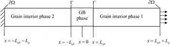
As mentioned in the previous section, it is assumed that for the nanoscale  . From a theoretical point of view, deformation is taken to occur in the following stages: (i) initially the whole material deforms elastically, (ii) after the initial elastic deformation, the GB will yield providing a knee in the stress–strain curve. GB yielding is assumed to occur due to sliding, rotation, and diffusion, as mentioned in the introduction. (iii) If deformation is sufficient, the GI phase will also yield at a critical load and a strain burst will occur (in Ref. Reference Schiotz, Vegge, Di Tolla and Jacobsen18, it is stated that some plastic deformation occurs in the grains). It should be noted that upon grain yielding, deformation will become perfectly plastic since it has been observed that deformation in grains at the nanoscale occurs through shear band formation, which corresponds to perfect plasticity.Reference Carsley, Ning, Milligan, Hackney and Aifantis13 (iv) Finally, increasing further the applied load, it is possible for some hardening to take place, after this perfectly plastic response, however, the simulations did not extend to such loads and rehardening after perfect plasticity did not occur.
In Ref. Reference Zhang and Aifantis34, the stress–strain responses for each of the aforementioned deformation stages were found, using the previously described gradient plasticity framework, Eqs. (1)–(6), but the plastic potential V was taken to be  . In particular, during the initial elastic deformation the stress–strain relationship was found as
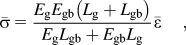
where (E g, E gb) denote the elastic moduli,  is the total strain and L = L g + L gb. After the GB phase yielded, a “knee” is observed in the stress–strain plot and the stress was given as

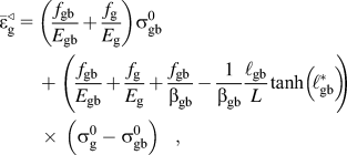
where  . With continuous deformation, the GI also began to deform in a perfectly plastic manner, through shear band formation,Reference Carsley, Ning, Milligan, Hackney and Aifantis13 when the strain was equal to
where f i = L i/L. Finally, for sufficient high deformation, re-hardening could occur after the grain yielded, according to
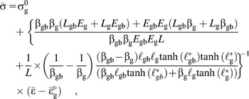
with  representing the starting strain of GI hardening

The difference of the strain before and after the strain burst will give the magnitude of the plateau, indicating perfect plasticity, as
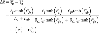
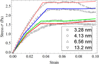
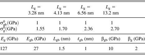
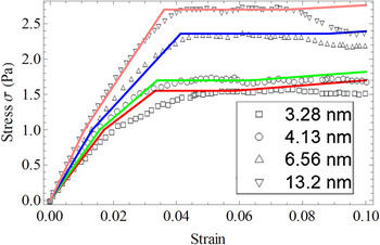
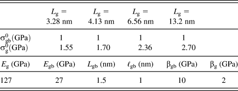
The aforementioned stress–strain curves have been plotted qualitatively,Reference Zhang and Aifantis34 but no comparison was performed with simulation dataReference Schiotz, Vegge, Di Tolla and Jacobsen18; here however, the above equations are directly fit to stress–strain curvesReference Schiotz, Vegge, Di Tolla and Jacobsen18 in Fig. 4. It can be seen that in the simulations there is no strain hardening stage after the plateau due to the computational cost. The material parameters that were chosen here, therefore, (Table II) allow for a large strain burst during grain yielding and minimal hardening after the burst, to fit the simulation profile. The fits obtained are indeed in agreement with,Reference Schiotz, Vegge, Di Tolla and Jacobsen18 and it should be noted that is the first time that a continuum theoretical model can capture this behavior. Finally, it can be noted that the same plasticity mechanisms of GB sliding were used to predict the flow stress in nanocrystalline Cu when the grain size was 10 nm.Reference Ovid'ko and Sheinerman22 It would be interesting to use the model ofReference Ovid'ko and Sheinerman22 with varying grain sizes and see if similar size effects as those of Fig. 4 are obtained.
Fit of theoretical model to MD simulations.Reference Schiotz, Vegge, Di Tolla and Jacobsen18
The fitting parameters for Fig .4.
IV. CONCLUSIONS
It was illustrated that gradient plasticity can be conveniently used to interpret GB hardening and softening as the grain size crosses over from the micrometer to the nanometer regime, by allowing grain boundaries to have a finite thickness, and a lower yield stress from the grains. In particular, an analytical expression is obtained for the critical grain size at which the “micro” to “nano” transition in deformation mechanisms occurs, and very good fits are performed to experimental data for the hardness dependence on the grain size. Furthermore, it is shown for the first time that gradient plasticity can effectively capture the softening in the flow stress of nanocrystalline Cu that has been observed in atomistic simulations.Reference Schiotz, Vegge, Di Tolla and Jacobsen18
ACKNOWLEDGMENT
The authors are grateful to KEA’s European Research Council Starting Grant MINATRAN 211166 for its support.