



1. Introduction
As one of the non-Newtonian fluids, viscoelastic fluids exist widely in nature (such as muds, blood, mantle, polymer solutions, etc.), and are significantly used in industry, e.g. enhancing fluid mixing (Groisman & Steinberg Reference Groisman and Steinberg2001), energy storage (Kang et al. Reference Kang, Kim, Song, Hong, Kim, Goh, Chung and Lee2023), heat transport enhancement (Boffetta et al. Reference Boffetta, Mazzino, Musacchio and Vozella2010) and turbulent drag reduction (White & Mungal Reference White and Mungal2008; Xi Reference Xi2019). Especially, turbulent drag can be greatly reduced in viscoelastic fluids containing a minute addition of polymers. Therefore, viscoelastic flows have attracted much attention from researchers for a long time.
1.1. Investigations of modal instabilities in viscoelastic parallel shear flows
For the transition to turbulence in parallel shear flows, Newtonian pipe flow is always linearly stable, and turbulence can only arise from perturbations of finite amplitude (Reynolds Reference Reynolds1883; Davey & Drazin Reference Davey and Drazin1969), while Garg et al. (Reference Garg, Chaudhary, Khalid, Shankar and Subramanian2018) first demonstrated that the viscoelastic pipe flow in dilute polymer solutions can be linearly unstable. Specifically, in viscoelastic pipe flow, the phase speed of the most unstable mode is close to the maximum propagation speed of the base flow at the pipe centreline, so this mode is named the centre mode. It should be remarked that the viscoelastic centre mode instability was actually observed earlier in viscoelastic Kolmogorov flow (Boffetta et al. Reference Boffetta, Celani, Mazzino, Puliafito and Vergassola2005). In viscoelastic plane Poiseuille flow, Khalid et al. (Reference Khalid, Chaudhary, Garg, Shankar and Subramanian2021a) also identified the unstable centre mode, and its linear instability threshold Re c (critical Reynolds number) is much lower than that of Newtonian plane Poiseuille flow, i.e. the threshold of Tollmien–Schlichting (TS) wave instability, and the typical structure of the centre mode can be clearly recognised in elasto-inertial turbulence investigations using direct numerical simulation (DNS) (Page et al. Reference Page, Dubief and Kerswell2020) and experiment (Choueiri et al. Reference Choueiri, Lopez, Varshney, Sankar and Hof2021). Khalid et al. (Reference Khalid, Shankar and Subramanian2021b) and Buza et al. (Reference Buza, Page and Kerswell2022) further indicated that the linear instability at Re = 0 can be the centre mode instability, and in numerical simulations of elastic turbulence (at very low Re), Berti & Boffetta (Reference Berti and Boffetta2010) and Lellep et al. (Reference Lellep, Linkmann and Morozov2024) also observed the typical flow structure of the centre mode. Therefore, a continuous pathway of centre mode instability from Re = 0 to Re ∼ O(103) exists, and whether at high or low Re, the centre mode instability can be viewed as purely elastic in origin (Buza et al. Reference Buza, Page and Kerswell2022), evidenced by the zero kinetic energy contribution from the base flow. When the finite extensibility of the polymer is considered, Khalid et al. (Reference Khalid, Badoni, Dutta, Naidu, Subramanian and Shankar2025) indicated that the finite extensibility plays a stabilising role for the FENE-CR model, and for the FENE-P model at relatively low elasticity number E (the ratio of the Weissenberg number to the Reynolds number), while at higher E values, finite extensibility destabilises the centre mode.
Based on the centre mode instability, Page et al. (Reference Page, Dubief and Kerswell2020), Morozov (Reference Morozov2022), Dubief et al. (Reference Dubief, Page, Kerswell, Terrapon and Steinberg2022) and Lellep et al. (Reference Lellep, Linkmann and Morozov2023) isolated and identified the exact coherent structures—nonlinear travelling-wave solutions with ‘arrowhead’ characteristics, which were suggested to organise the phase-space dynamics of purely elastic and elasto-inertial chaotic channel flows at very high elasticity. However, the dynamical origins of elasto-inertial turbulence remain complex. Beneitez et al. (Reference Beneitez, Page, Dubief and Kerswell2024) indicated that, in two dimensions, this arrowhead structure is disconnected from the self-sustaining mechanisms of elasto-inertial turbulence, and to trigger any chaotic motion, the near-wall viscoelastic TS wave mechanism (Shekar et al. Reference Shekar, Mcmullen, Wang, McKeon and Graham2019; Zhang et al. Reference Zhang, Cheng, Wang, Zhang, Li and Li2024) may be operative, which will be discussed below in detail. Besides, Lellep, Linkmann & Morozov (Reference Lellep, Linkmann and Morozov2023, Reference Lellep, Linkmann and Morozov2024) indicated that a three-dimensional route to elasto-inertial turbulence stemming from the arrowhead structure cannot be ruled out. Using numerical simulation, Foggi Rota et al. (Reference Foggi Rota, Amor, Le Clainche and Rosti2024) demonstrated that the fully developed turbulent state arising after the transition (including elastic turbulence states and many elasto-inertial turbulences) shares a similar structure once inertial effects are subdominant, reflecting the transition continuity between these two types of turbulence in some cases.
On the other hand, at higher Reynolds numbers and lower polymer elasticity, it is important to note that, in inertia-dominated viscoelastic flow, viscoelasticity modifies the linear instability threshold of the TS mode (Sureshkumar & Beris Reference Sureshkumar and Beris1995; Sadanandan & Sureshkumar Reference Sadanandan and Sureshkumar2002; Zhang et al. Reference Zhang, Lashgari, Zaki and Brandt2013). Specifically, these results indicated that the non-zero solvent viscosity stabilises the viscoelastic flow, and the instability threshold Re c varies non-monotonically with the Weissenberg number W. Besides, Chaudhary et al. (Reference Chaudhary, Garg, Shankar and Subramanian2019) further performed a comprehensive study of wall mode instabilities by using the viscoelastic UCM model (a limiting case of the Oldroyd-B model without solvent viscosity), and seven unstable modes were identified, including the original TS mode; see their results in detail. Shekar et al. (Reference Shekar, Mcmullen, Wang, McKeon and Graham2019, Reference Shekar, Mcmullen, Wang, McKeon and Graham2020) observed localised polymer stretch fluctuations and the corresponding sheet-like extension structure near the wall in simulations of elasto-inertial turbulence, which are similar to the structures arising from the TS mode. Furthermore, they demonstrated that this nonlinear TS wave-like structure is a solution branch caused by viscoelasticity and is not connected to the nonlinear TS solution branch found for Newtonian flow. Zhang et al. (Reference Zhang, Cheng, Wang, Zhang, Li and Li2024) further indicated that two-dimensional elasto-inertial turbulence originates from this sheet-like structure, and the key mechanisms for the self-sustaining of elasto-inertial turbulence are manifested as the fracture and regeneration of this sheet-like structure. From the perspective of spectral proper orthogonal decomposition (Kumar & Graham Reference Kumar and Graham2024), the travelling-wave structures with different frequencies are nested within each other in elasto-inertial turbulence, and the sheetlike localised stress fluctuations prevent velocity fluctuations from penetrating them. For plane Couette flow, another classic parallel shear flow, the flow is always linearly stable in both Newtonian and viscoelastic fluids (Schmid & Henningson Reference Schmid and Henningson2001; Chaudhary et al. Reference Chaudhary, Garg, Shankar and Subramanian2019). However, recently, Beneitez et al. (Reference Beneitez, Page and Kerswell2023) identified the linear instability mode in plane Couette flow by adding ‘artificial’ polymer diffusion to the governing equation, although the reality and reliability of this polymer diffusion instability need to be further investigated. Notably, Dong & Wan (Reference Dong and Wan2025) indicated that this new instability is induced by the conformation boundary conditions additionally introduced in the artificial conformation diffusion equation system, and can be eliminated by adopting new boundary conditions on the conformation tensor without affecting other types of instabilities.
1.2. Investigations of non-modal instabilities in viscoelastic parallel shear flows
In wall-bounded shear flows, due to the significant algebraic growth of perturbation energy caused by the non-normality of the linear operators (Trefethen et al. Reference Trefethen, Trefethen, Reddy and Driscoll1993; Schmid & Henningson Reference Schmid and Henningson2001; Schmid Reference Schmid2007), it is difficult to describe the transition scenario accurately by modal theory, even when the flow is linearly stable. This energy growth can serve as an initial stage of the development of streamwise elongated flow structures, which may undergo secondary amplification (Schoppa & Hussain Reference Schoppa and Hussain2002) or nonlinear instability (Waleffe Reference Waleffe1997) when a finite amplitude is reached, and thereby provide a bypass transition to turbulence at a lower Re (Klebanoff et al. Reference Klebanoff, Tidstrom and Sargent1962). In addition, non-modal analysis can also provide the key linear mechanism to reveal and understand self-sustained processes in turbulence (Duriez et al. Reference Duriez, Aider and Wesfreid2009; Lozano-Durán et al. Reference Lozano-Durán, Constantinou, Nikolaidis and Karp2021; Markeviciute & Kerswell Reference Markeviciute and Kerswell2024), and can offer the input–output viewpoint in flow control (Jovanović Reference Jovanović2021). Therefore, our work focuses on the initial phase of the disturbance evolution, and the amplitude of the disturbance at this stage can be assumed to be small. Next, we review the research progress related to non-modal transient growth.
In Newtonian channel flows, Reddy & Henningson (Reference Reddy and Henningson1993) found that streamwise-uniform disturbances, i.e. the streamwise wavenumber is set to 0, achieve the largest energy growth, so the non-modal instability exhibits a three-dimensional nature. The reason for this energy growth is called the lift-up mechanism (Schmid & Henningson Reference Schmid and Henningson2001), and specifically, streamwise vortices drive low-energy fluids near the boundaries into regions of faster mean flow so as to form streamwise streaks, thus causing energy release from the mean shear to the perturbed wall-normal vorticity. In plane Poiseuille/Couette flow of viscoelastic fluids, Hoda, Jovanović & Kumar (Reference Hoda, Jovanović and Kumar2008) firstly investigated the growth of disturbance kinetic energy excited by a stochastic forcing. Their results suggested that streamwise elongated structures, i.e. streamwise streaks, generally have the largest energy growth, and increasing the elasticity number or decreasing the viscosity ratio can significantly enhance the energy amplification, with the optimal spanwise wavenumber to achieve the maximum energy amplification increasing simultaneously. Compared with Newtonian fluids, such a large transient growth in viscoelastic fluids is caused by the energy exchange between the streamwise/wall-normal component of the polymeric stresses and the wall-normal gradient of the streamwise velocity (Hoda, Jovanović & Kumar Reference Hoda, Jovanović and Kumar2009). Besides, it should be noted that viscoelasticity cannot always lead to the enhancement of non-modal instability, and specifically, Zhang et al. (Reference Zhang, Lashgari, Zaki and Brandt2013) indicated that, using the FENE-P model, the energy growth of oblique disturbances in a viscoelastic fluid is smaller than that in a Newtonian fluid. For the streak evolution in viscoelastic fluids, Page & Zaki (Reference Page and Zaki2014) found that there are two distinct responses of wall-normal vorticity in Oldroyd-B plane Couette flow, one is termed the quasi-Newtonian case, and the other is termed the elastic case, where streaks can reach significant amplitudes even at very weak inertia.
The above investigations have primarily focused on the kinetic energy growth induced by velocity disturbances, and an early work on the transient growth caused by elastic disturbances was conducted by Jovanović & Kumar (Reference Jovanović and Kumar2010). Their results showed that, in streamwise-constant creeping flows of strong elasticity, the fluctuations in the streamwise component of the polymer stress tensor achieve O(W 2) growth, and the fluctuations in streamwise velocity achieve O(W) growth (we reiterate that W represents the Weissenberg number). In terms of physical mechanisms, Jovanović & Kumar (Reference Jovanović and Kumar2010) roughly attributed the reason for this growth to the polymer stretching caused by the background shear, and mathematically, Kupferman (Reference Kupferman2005) and Hariharan, Jovanović & Kumar (Reference Hariharan, Jovanović and Kumar2021) concluded that the continuous spectrum is possibly associated with a strong transient growth in the linear framework. In addition, Doering et al. (Reference Doering, Eckhardt and Schumacher2006) demonstrated that, by constructing exact solutions to the full two-dimensional nonlinear equations, the conventional nonlinear energy stability fails for Oldroyd-B fluids at arbitrarily low Reynolds numbers, and they showed examples of some perturbations that exhibit transient energy growth. Using a localised measure of disturbance amplification instead of square-integrated quantities (corresponding to typical non-modal analysis), Hariharan, Jovanović & Kumar (Reference Hariharan, Jovanović and Kumar2021) found that, at very weak shear strength, spanwise-uniform (the spanwise wavenumber is set to 0) stress fluctuations are more amplified than streamwise-uniform stress fluctuations, and the amplification of velocity fluctuations can be negligible compared with the amplification of elastic stress fluctuations, which indicates that the amplification of elastic disturbances in a strongly elastic fluid may exhibit two-dimensional characteristics. Besides, the exact coherent structure and the associated self-sustaining mechanism in both elastic turbulence (Morozov Reference Morozov2022; Lellep et al. Reference Lellep, Linkmann and Morozov2023) and elasto-inertial turbulence (Sid et al. Reference Sid, Terrapon and Dubief2018; Shekar et al. Reference Shekar, Mcmullen, Wang, McKeon and Graham2019; Page et al. Reference Page, Dubief and Kerswell2020; Khalid et al. Reference Khalid, Chaudhary, Garg, Shankar and Subramanian2021a ) associated with transient growth all exhibit a (quasi) two-dimensional nature. This self-sustaining mechanism and the associated attractor in elasto-inertial turbulence can emerge through transient growth (Page & Zaki Reference Page and Zaki2014; Shekar et al. Reference Shekar, Mcmullen, Mckeon and Graham2020). In a recent experiment, Shnapp & Steinberg (Reference Shnapp and Steinberg2022) observed the non-modal elastic instability and further illustrated that the weak disturbances (but still of finite amplitude) can generate the elastic instability and the subsequent elastic turbulence in channel flow, which also greatly motivates the present study.
More recently, Hameduddin et al. (Reference Hameduddin, Meneveau, Zaki and Gayme2018, Reference Hameduddin, Gayme and Zaki2019) indicated that, in the problem of formulating perturbative expansions of the polymer conformation tensor, the traditional Reynolds decompositions do not explicitly take into account that the perturbed tensor must remain positive definite, so a new geometric decomposition and the associated scalar measures of the polymer fluctuations were proposed, including a clear physical interpretation of polymer deformation and the associated disturbance elastic energy, which promote the development of related research on viscoelastic instability. In the previous non-modal instability investigations (e.g. Doering et al. Reference Doering, Eckhardt and Schumacher2006; Jovanović & Kumar Reference Jovanović and Kumar2010; Hariharan, Jovanović & Kumar Reference Hariharan, Jovanović and Kumar2021), the square-integrated perturbation polymer stress (associated with the classical Reynolds decomposition) does not correspond to a proper norm in the obvious fashion that the kinetic energy does, and the related transient growth results are opposite to those obtained by directly measuring growth using the maximum perturbation polymer stress, which is likely due to the lack of correct inner products and associated norms in the perturbation elastic energy, and thus unwittingly conceal the difficulties in the research of viscoelastic non-modal instability. Based on new geometric perturbative expansions, Zhang (Reference Zhang2021) studied the transient growth of high-Re viscoelastic pipe flows. To the best of our knowledge, this is the first application of such an expansion in non-modal analysis. The results showed that, unlike the Newtonian case (Schmid & Henningson Reference Schmid and Henningson2001), here, the helical mode undergoes a greater energy growth and is larger than that of the axisymmetric mode, and the stronger elastic effect leads to a greater amplitude of the optimal conformation tensor in the pipe central region. Besides, using this new definition of disturbance elastic energy, Wan et al. (Reference Wan, Sun and Zhang2021) and Buza et al. (Reference Buza, Page and Kerswell2022) determined the bifurcation types of the onset of elastic instability in viscoelastic pipe flow and plane Poiseuille flow, respectively. In particular, Wan et al. (Reference Wan, Sun and Zhang2021) found that the transition from supercritical to subcritical bifurcation occurs at a viscosity ratio of β = 0.785, which is close to the experimental bifurcation point at β = 0.855.
1.3. The position of the current work
As reviewed above, investigations on the non-modal transient energy growth of viscoelastic channel flow considering elastic disturbances have only received preliminary exploration and are mostly limited to the extremely low Reynolds number region. Consequently, linear non-modal instabilities over a wide range of Re (from O(10−2) to O(103)) are not yet well understood, which limits our understanding of the early transition to elastic and elasto-inertial turbulent states. In addition, the related physical models suffer from certain deficiencies when the perturbation elastic energy is measured by Reynolds decomposition in non-modal analysis, so the associated energy growth mechanism has not been clearly explained. From the new perspective of geometric decomposition with a clear physical interpretation (Hameduddin et al. Reference Hameduddin, Meneveau, Zaki and Gayme2018, Reference Hameduddin, Gayme and Zaki2019), few researchers have studied non-modal instabilities and related problems, except for the works of Shekar et al. (Reference Shekar, Mcmullen, Mckeon and Graham2020), Zhang (Reference Zhang2021), Wan et al. (Reference Wan, Sun and Zhang2021) and Buza et al. (Reference Buza, Page and Kerswell2022), etc., and the most relevant work is Zhang (Reference Zhang2021), studying the transient growth in high-Re viscoelastic pipe flow. In the current work, motivated by Zhang (Reference Zhang2021), we perform a comprehensive linear non-modal stability analysis of plane Poiseuille flows (of Oldroyd-B fluids, and FENE-P fluids in Appendix B) based on a new geometric decomposition of the polymer conformation tensor. The significance of the current work lies in (i) supplementing the works by Jovanović & Kumar (Reference Jovanović and Kumar2010) and Hariharan, Jovanović & Kumar (Reference Hariharan, Jovanović and Kumar2021) on the preliminary exploration of the energy growth of viscoelastic plane shear flows at low Re, by using the new disturbance decomposition; (ii) extending the Reynolds number into a large range (from Re = 0.01 to Re = 1000) to understand the non-modal instabilities in both elastic and elasto-inertial turbulence states and the transition between them; and (iii) providing the mechanisms of transient growth by using input–output analysis, optimal response/initial conditions and transient energy analysis, etc.
The rest of the paper is organised as follows. In § 2, we introduce the physical problem, the governing equations, the non-dimensional parameters and the two transient energy growth methods. In § 3, the numerical method and code validation are briefly presented. We present the results in § 4, including transient growth that is affected by various non-dimensional parameters, and underlying growth mechanisms studied by input–output analysis, elastic/kinetic energy analysis and optimal response/initial conditions. We conclude the paper in § 5 with some discussions on the results.
2. Problem formulation
2.1. Theoretical modelling
Figure 1 shows the schematic of viscoelastic channel flow. The upper and lower plates extend infinitely in the x (streamwise) and z (spanwise) directions. Regarding the viscoelastic effects, except for some results for the FENE-P fluid shown at the end of § 4.2, we mainly consider an Oldroyd-B fluid, which focuses on the interaction between polymers and hydrodynamic fluctuations and can capture the essential instability mechanism in the flow.
Schematic description of the problem.

Based on Bird et al. (Reference Bird, Curtiss, Armstrong and Hassager1987) and Larson (Reference Larson1988), to non-dimensionalise the governing equations of viscoelastic flow, we introduce the following scalings:
 \begin{align} \left(x,y,z\right)=\frac{\left(x^{*},y^{*},z^{*}\right)}{H^{*}} ,\,\,\,\boldsymbol{U}=\frac{\boldsymbol{U}^{*}}{{U}_{0}^{*}} ,\,\, t=t^{*}/\left(\frac{H^{*}}{{U}_{0}^{*}}\right) ,\quad P=\frac{P^{*}}{\rho ^{*}{U}_{0}^{*^{2}}} ,\,\, \boldsymbol{C}=\frac{\boldsymbol{C}^{*}}{{k}_{B}^{*}T^{*}/h^{*}} , \end{align}
where H
* is the half-distance between the two plates,
U
* = [U
*, V
*, W
*] is the velocity of the liquid, t
* is time, P
* is the pressure, ρ
* is the liquid density,
 $U_0^*$
is the centreline velocity of the base flow,
 $\kappa_{\textrm{B}}^*$
is the Boltzmann constant, T
* is the temperature,
C
* is the polymer conformation tensor and h
* is the spring constant (the superscript * indicates a dimensional variable). Therefore, the governing equations are non-dimensionalised as follows:
 \begin{align} \boldsymbol{\nabla }\boldsymbol{\cdot }\boldsymbol{U}=0 , \end{align}
 \begin{align} \frac{\partial \boldsymbol{U}}{\partial t}+\left(\boldsymbol{U}\boldsymbol{\cdot }\boldsymbol{\nabla }\right)\boldsymbol{U}=-\boldsymbol{\nabla }P+\frac{\beta }{Re}\boldsymbol{\nabla} ^{2}\boldsymbol{U}+\frac{1-\beta }{ReW}\boldsymbol{\nabla }\boldsymbol{\cdot }\boldsymbol{C} , \end{align}
 \begin{align} \frac{\partial \boldsymbol{C}}{\partial t}+\boldsymbol{U}\boldsymbol{\cdot }\boldsymbol{\nabla }\boldsymbol{C}-\boldsymbol{C}\boldsymbol{\cdot }\boldsymbol{\nabla }\boldsymbol{U}-\left(\boldsymbol{\nabla }\boldsymbol{U}\right)^{T}\boldsymbol{\cdot }\boldsymbol{C}=-\frac{\boldsymbol{C}-\boldsymbol{I}}{W} , \end{align}
where three dimensionless parameters appear, and their specific definitions are
 \begin{align} Re=\frac{\rho ^{*}{U}_{0}^{*}H^{*}}{\mu ^{*}} ,\quad\beta =\frac{{\mu }_{s}^{*}}{\mu ^{*}} ,\quad W=\frac{\lambda ^{*}{U}_{0}^{*}}{H^{*}} . \end{align}
Here, Re is the Reynolds number, which measures the relative importance of the inertia force to the viscous force; β is the viscosity ratio, defined as the ratio of the solvent viscosity
 $\mu_s^*$
to the total viscosity μ
* (μ
* =
 $\mu_s^*$
+
 $\mu_p^*$
, and
 $\mu_p^*$
is the dynamic viscosity of polymer), and a smaller β denotes a higher concentration of polymer additives; W is the Weissenberg number which represents the ratio of the relaxation time of the polymer (λ
*) to the flow convective time scale (H
*/
 $U_0^*$
).
The dimensionless boundary conditions are U (y = ±1) = 0, and the perturbation boundary conditions of the conformation tensor C are not required since there are no terms involving derivatives of these stresses with respect to y (Hoda, Jovanović & Kumar Reference Hoda, Jovanović and Kumar2008; Zhang et al. Reference Zhang, Lashgari, Zaki and Brandt2013).
2.2. Linearisation
We decompose the flow variable into the sum of the base state and perturbation, and the linear system reads
 \begin{align} \boldsymbol{\nabla }\boldsymbol{\cdot }\boldsymbol{u}=0 , \end{align}
 \begin{align} \frac{\partial \boldsymbol{u}}{\partial t}+\left(\overline{\boldsymbol{U}}\boldsymbol{\cdot }\boldsymbol{\nabla }\right)\boldsymbol{u}+\left(\boldsymbol{u}\boldsymbol{\cdot }\boldsymbol{\nabla }\right)\overline{\boldsymbol{U}}=-\boldsymbol{\nabla }p+\frac{\beta }{Re}\boldsymbol{\nabla} ^{2}\boldsymbol{u}+\frac{1-\beta }{ReW}\boldsymbol{\nabla }\boldsymbol{\cdot }\boldsymbol{c} , \end{align}
 \begin{align} \frac{\partial \boldsymbol{c}}{\partial t}+\overline{\boldsymbol{U}}\boldsymbol{\cdot }\boldsymbol{\nabla }\boldsymbol{c}+\boldsymbol{u}\boldsymbol{\cdot }\boldsymbol{\nabla }\overline{\boldsymbol{C}}-\overline{\boldsymbol{C}}\boldsymbol{\cdot }\boldsymbol{\nabla }\boldsymbol{u}-\boldsymbol{c}\boldsymbol{\cdot }\boldsymbol{\nabla }\overline{\boldsymbol{U}}-\left(\boldsymbol{\nabla }\boldsymbol{u}\right)^{T}\boldsymbol{\cdot }\overline{\boldsymbol{C}}-\left(\boldsymbol{\nabla }\overline{\boldsymbol{U}}\right)^{T}\boldsymbol{\cdot }\boldsymbol{c}=-\frac{\boldsymbol{c}}{W} , \end{align}
where the uppercase letters with a horizontal bar above represent the base state quantity, the lowercase letters are perturbations and the boundary conditions of perturbations are: u (y = ±1) = 0.
From (2.4), we can deduce that the base conformation tensor is
 \begin{align} \overline{\boldsymbol{C}}=\left(\!\begin{array}{ccc} 2W^{2}{\overline{U}^{\prime}}^{2}+1 & W\overline{U}^{\prime} & 0\\ W\overline{U}^{\prime} & 1 & 0\\ 0 & 0 & 1 \end{array}\!\right)\!. \end{align}
To better measure polymer deformation and the associated perturbation elastic energy, we employ the new geometric decomposition of the polymer conformation tensor introduced by Hameduddin et al. (Reference Hameduddin, Meneveau, Zaki and Gayme2018, Reference Hameduddin, Gayme and Zaki2019). The key physical idea of choosing this decomposition is that, instead of using
 $\boldsymbol{C}-\overline{\boldsymbol{C}}$
as the definition of the deformation of the polymers, one should use
 $\log (\overline{\boldsymbol{H}}^{-1}\boldsymbol{\cdot }\boldsymbol{C}\boldsymbol{\cdot }(\overline{\boldsymbol{H}}^{\dagger} )^{-1})$
, where
 $\overline{\boldsymbol{C}}= \overline{\boldsymbol{H}}\,\overline{\boldsymbol{H}}^{\dagger}$
, a Cholesky decomposition of the base state of the conformation tensor, and the superscript † stands for the conjugate transpose. Specifically, in the linear phase, the geometric decomposition of the polymer conformation tensor in the additive form is
 $\boldsymbol{G}= \overline{\boldsymbol{G}}+\boldsymbol{g}$
(where the base state satisfies
 $\overline{\boldsymbol{G}}= \boldsymbol{I}$
, and
I
is the identity matrix) compared with the classical Reynolds decomposition
 $\boldsymbol{C}= \overline{\boldsymbol{C}}+\boldsymbol{c}$
, which guarantees that the new perturbed conformation tensor field remains positive definite and provides the volume-averaged squared geodesic distance between
C
and
 $\overline{\boldsymbol{C}}$
by tr(
g
2). The conversion between the perturbation conformation tensor
c
and
g
is
 $\boldsymbol{c}=\overline{\boldsymbol{H}}\boldsymbol{\cdot }\boldsymbol{g}\boldsymbol{\cdot }\overline{\boldsymbol{H}}^{\dagger }$
, and its explicit expression
c
vec
=
Qg
vec
in the vector form (
g
vec
= (g
xx
, g
yy
, g
zz
, g
xy
, g
xz
, g
yz
)T) is (see also Zhang (Reference Zhang2021))
 \begin{align} \!\!\left(\begin{array}{l} c_{xx}\\ c_{yy}\\ c_{zz}\\ c_{xy}\\ c_{xz}\\ c_{yz} \end{array}\right){=}\underset{\boldsymbol{Q}}{\underbrace{\left(\!\begin{array}{cccccc} \overline{S}^{2}/\overline{C}_{yy} & {\overline{C}}_{xy}^{2}/\overline{C}_{yy} & 0 & 2\overline{S}\,\overline{C}_{xy}/\overline{C}_{yy} & 0 & 0\\ 0 & \overline{C}_{yy} & 0 & 0 & 0 & 0\\ 0 & 0 & \overline{C}_{zz} & 0 & 0 & 0\\ 0 & \overline{C}_{xy} & 0 & \overline{S} & 0 & 0\\ 0 & 0 & 0 & 0 & \sqrt{\frac{\overline{C}_{zz}}{\overline{C}_{yy}}}\overline{S} & \sqrt{\frac{\overline{C}_{zz}}{\overline{C}_{yy}}}\overline{C}_{xy}\\ 0 & 0 & 0 & 0 & 0 & \sqrt{\overline{C}_{yy}\overline{C}_{zz}} \end{array}\!\right)}}\left(\!\begin{array}{l} g_{xx}\\ g_{yy}\\ g_{zz}\\ g_{xy}\\ g_{xz}\\ g_{yz} \end{array}\!\right) , \end{align}
where
 $\overline{S}=\sqrt{\overline{C}_{yy}\overline{C}_{xx}-{\overline{C}}_{xy}^{2}}$
.
Note that the completely geometric perturbative expansion is required in a full Riemannian manifold Pos 3 (Pos 3 is non-Euclidean), while in the local tangent space of Pos 3, the Riemannian metric can be reduced to the Euclidean inner products. Therefore, using the Frobenius norm to calculate non-modal transient growth is justified in the linear regime (where the expansion is implemented in the tangent space of Pos 3), while the full Riemannian metric is necessary when a finite amplitude perturbation in nonlinear non-modal analysis is considered (Kerswell Reference Kerswell2018).
Since the flow is homogeneous in the streamwise and spanwise directions, it is assumed that the perturbations are wave-like (periodic in these two directions), i.e.
 \begin{align} f\left(x,y,z,t\right)=\tilde{f}\left(y,t\right)e^{\left(i\alpha x+i\gamma z\right)}=\hat{f}\left(y\right)e^{-i\omega t}e^{\left(i\alpha x+i\gamma z\right)} , \end{align}
where f can be an arbitrary perturbation, the real-valued α and γ are streamwise and spanwise wavenumbers, respectively,
 $\tilde{\text{ f}}$
and
 $\hat{\text{ f}}$
are the shape functions and ω is the complex frequency of disturbance, with its imaginary part ω
i
representing the growth rate of linear disturbance (if ω
i > 0, the fluid system is linearly unstable for t → ∞, and ω
i < 0 indicates a stable flow).
Using the wall-normal vorticity η = ∂u/∂z − ∂w/∂x to eliminate the pressure term in (2.6–2.8) and using the transformation between c and g in (2.10), we obtain the linear stability equation of the following form:
 \begin{align} \boldsymbol{A}\frac{\partial \tilde{\boldsymbol{\chi }}}{\partial t}=\boldsymbol{B}\tilde{\boldsymbol{\chi }} , \end{align}
where
 $\tilde{\boldsymbol{\chi }}$
= (
 $\tilde{\text{ v}}$
,
 $\tilde{\eta }$
,
 $\tilde{\text{ g}}$
xx
,
 $\tilde{\text{ g}}$
yy
,
 $\tilde{\text{ g}}$
zz
,
 $\tilde{\text{ g}}$
xy
,
 $\tilde{\text{ g}}$
xz
,
 $\tilde{\text{ g}}$
yz
), the elements in matrices
A
and
B
can be found in (A3–A10) of Appendix A, and the boundary conditions are:
 \begin{align} \tilde{v}\left(\pm 1,t\right)=0,\quad\tilde{v}^{\prime}\left(\pm 1,t\right)=0,\quad\tilde{\eta }\left(\pm 1,t\right)=0 . \end{align}
2.3. Transient energy growth
In our calculation of the non-modal transient growth, following the definition of perturbation elastic energy (Min et al. Reference Min, Yoo, Choi and Joseph2003; Dallas et al. Reference Dallas, Vassilicos and Hewitt2010; Zhang Reference Zhang2021), we define the total energy density of the perturbation contained in a control volume as
 \begin{align} \int _{\varOmega }\varepsilon \text{d}V=\int _{\varOmega }\left(\varepsilon _{k}+\varepsilon _{p}\right)\text{d}V & =\frac{1}{2}\int _{\varOmega }\left[\left(\left| \tilde{u}\right| ^{2}+\left| \tilde{v}\right| ^{2}+\left| \tilde{w}\right| ^{2}\right)+\frac{1-\beta }{ReW}tr\left(\tilde{\boldsymbol{g}}^{2}\right)\right]\text{d}V\nonumber\\ &=\int _{\varOmega }\tilde{\boldsymbol{\chi }}\boldsymbol{M}\tilde{\boldsymbol{\chi }}^{\dagger }\text{d}V , \end{align}
where Ω = 2ab, a = 2π/α, b = 2π/γand ε k , ε p and ε denote the perturbation kinetic energy, perturbation elastic energy and total energy, respectively.
The details of the energy weight matrix M are given as
 \begin{align} \boldsymbol{M}&=\frac{1}{2}diag\left(\boldsymbol{I}+\frac{1}{k^{2}}{\boldsymbol{D}}_{1}^{\dagger }\boldsymbol{D}_{1},\frac{1}{k^{2}}\boldsymbol{I},\frac{1-\beta }{ReW}\boldsymbol{I},\frac{1-\beta }{ReW}\boldsymbol{I},\frac{1-\beta }{ReW}\boldsymbol{I},\frac{2\left(1-\beta \right)}{ReW}\boldsymbol{I},\right.\nonumber\\ &\quad\left.\frac{2\left(1-\beta \right)}{ReW}\boldsymbol{I}, \frac{2\left(1-\beta \right)}{ReW}\boldsymbol{I}\right) , \end{align}
where k 2 = α 2 + γ 2 and D 1 denotes the first-derivative matrix with respect to the vertical direction y.
To calculate transient energy growth, two methods are employed: one is based on the eigenvalues and eigenvectors, and the other is entirely operator based. These two methods not only serve to cross-validate the results but also elucidate the mechanism of energy amplification from different perspectives.
Specifically, for the first method, we decompose
 $\tilde{\boldsymbol{\chi }}$
into a large, but finite number J of eigenvectors
 $\tilde{\boldsymbol{\chi }}$
j
of
L
(
L
=
A
−1
B
). We have
 \begin{align} \tilde{\boldsymbol{\chi }}=\sum\limits_{j=1}^{J}\kappa _{j}\tilde{\boldsymbol{\chi }}_{\!j} . \end{align}
Since only the first J eigenfunctions of L are considered, the problem now reduces to an initial value problem for the expansion coefficients κ j . Based on (2.11)–(2.12), we have
 \begin{align} \frac{d\boldsymbol{\kappa }}{\text{d}t}=-i\mathbf{\varLambda }\boldsymbol{\kappa } , \end{align}
where κ = (κ 1, κ 2, … , κ J ) and Λ = diag(ω 1,ω 2, … , ω J ), and the solution to (2.17) reads κ = κ 0e −iΛt ( κ 0 is the expansion coefficient at t = 0).
Equation (2.14) is rewritten as
 \begin{align*}\int _{\varOmega }\varepsilon \text{d}V\!{=}\int _{\varOmega }\tilde{\boldsymbol{\chi }}\boldsymbol{M}\tilde{\boldsymbol{\chi }}^{\dagger }\text{d}V\!{=}\!\int _{\varOmega }\left(\sum\limits_{j=1}^{J}\kappa _{j}\tilde{\boldsymbol{\chi }}_{j}\right)\boldsymbol{M}\left(\sum\limits_{e=1}^{J}\kappa _{e}\tilde{\boldsymbol{\chi }}_{e}\right)^{\dagger }\!\text{d}V{=}\sum\limits_{j,e=1}^{J}\kappa _{j}\boldsymbol{M}_{je}{\kappa }_{e}^{\dagger } , \end{align*}
 \begin{align}\textrm{with}\,\,\, \boldsymbol{M}_{\!je}=\int _{\varOmega }\tilde{\boldsymbol{\chi }}_{j}\boldsymbol{M}{\tilde{\boldsymbol{\chi }}}_{e}^{\dagger }\text{d}V . \end{align}
We perform the Cholesky decomposition on M je , i.e. M je = FF †, and define ζ = Fκ . Therefore, using Parseval’s identity, (2.18) becomes
 \begin{align} \int _{\varOmega }\varepsilon \text{d}V=\sum\limits_{j,e=1}^{J}\kappa _{j}\boldsymbol{M}_{\!je}{\kappa }_{e}^{\dagger }=\boldsymbol{\kappa }^{\dagger }\boldsymbol{F}^{\dagger }\boldsymbol{F}\boldsymbol{\kappa }=\left(\boldsymbol{F}\boldsymbol{\kappa }\right)^{\dagger }\boldsymbol{F}\boldsymbol{\kappa }={\left|\left|\boldsymbol{\zeta }\right|\right|}_{2}^{2} , \end{align}
where
 $\| \cdot\|_2$
represents the L
2-norm.
Based on (2.17), we also have the solution of ζ , i.e.
 \begin{align} \boldsymbol{\zeta }=\boldsymbol{\zeta }_{0}\exp \left(\!-i\boldsymbol{F}\mathbf{\varLambda }\boldsymbol{F}^{-1}t\right) , \end{align}
where ζ 0 is the initial ζ at t = 0.
Therefore, the transient growth G, optimised over all possible initial conditions, can be formulated as
 \begin{align} G\left(t\right)=\max\limits _{\boldsymbol{\zeta }_{0}}\frac{\| \boldsymbol{\zeta }| {| }_{2}^{2}}{\| \boldsymbol{\zeta }_{0}| {| }_{2}^{2}}=\left\| \exp \left(\!-i\boldsymbol{F}\mathbf{\varLambda }\boldsymbol{F}^{-1}t\right)\right\|_{2}^{2} . \end{align}
For the second method, this method evaluates the energy growth caused by the specified physical field, and an input–output analysis is typically combined. The different input filters B in and output filters C out are defined in tables 1 and 2, and their specific expressions are straightforward; see, for instance, Jovanović & Bamieh (Reference Jovanović and Bamieh2005) and Zhang et al. (Reference Zhang, Lashgari, Zaki and Brandt2013, Reference Zhang, Martinelli, Wu, Schmid and Quadrio2015).
The definition of input filters and the definition of their resulting transient growth, with C out fixed as C out-k,p .

Table 1. Long description
A table with 10 rows and 5 columns. The columns are labeled Type of input disturbance, (v, η), B-, and x-. The rows are grouped into Input filter and Transient growth. The first group has two rows: Input filter with B-in-k, B-in-p, B-in-k,p and Transient growth with Giv, η, Gi-g, G. The second group has nine rows: Type of input disturbance with xx, yy, zz, xy, xz, yz and Input filter with Bin1, Bin2, Bin3, Bin4, Bin5, Bin6, Bin7, Bin8 and Transient growth with Gi-v, Gi-η, Gi-gxx, Gi-gyy, Gi-gzz, Gi-gxy, Gi-gxz, Gi-gyz.
The definition of output filters and the definition of their resulting transient growth, with B in fixed as B in-k,p .

Table 2. Long description
The table is divided into two sections: input filters and output filters. Each section has rows labeled by the type of disturbance and columns labeled by the type of filter and transient growth. The first section, input filters, has three rows labeled by the type of input disturbance and columns labeled by the input filter and transient growth. The second section, output filters, has a similar structure with rows labeled by the type of output disturbance and columns labeled by the output filter and transient growth. Each row provides specific values for the filters and transient growth corresponding to the type of disturbance.
For the specific calculation of the second method, the input condition is
 $\tilde{\boldsymbol{\chi }}$
in
=
B
in
 $\tilde{\boldsymbol{\chi }}_{in}^{0}$
and the output is
 $\tilde{\boldsymbol{\chi }}$
out
=
C
out
 $\tilde{\boldsymbol{\chi }}_{out}^{0}$
, where
 $\tilde{\boldsymbol{\chi }}_{out}^{0}$
= e
t
L
 $\tilde{\boldsymbol{\chi }}$
in
= e
t
L
B
in
 $\tilde{\boldsymbol{\chi }}_{in}^{0}$
. Therefore, the output becomes
 $\tilde{\boldsymbol{\chi }}$
out
=
C
out
 $\tilde{\boldsymbol{\chi }}_{out}^{0}$
=
C
oute
t
L
B
in
 $\tilde{\boldsymbol{\chi }}_{in}^{0}$
. We redefine the output energy weight matrix
M
out
=
C
out
 $\boldsymbol{MC}_{out}^T$
and the input energy weight matrix
M
in
=
 $\boldsymbol{B}_{in}^T$
MB
in
. Reapplying a Cholesky decomposition to
M
in
and
M
out
,
M
in
=
 $\boldsymbol{F}_{in}^{\dagger}$
F
in
and
M
out
=
 $\boldsymbol{F}_{out}^{\dagger}$
F
out
, the energy growth with an input–output matrix is
 \begin{align} \begin{array}{ll} G\left(t\right) & =\max\limits _{{\tilde{\boldsymbol{\chi }}}_{in}^{0}}\frac{{\left|\left|\boldsymbol{F}_{out}\tilde{\boldsymbol{\chi }}_{out}\right|\right|}_{2}^{2}}{{\left|\left|\boldsymbol{F}_{in}{\tilde{\boldsymbol{\chi }}}_{in}^{0}\right|\right|}_{2}^{2}}=\max\limits _{{\tilde{\boldsymbol{\chi }}}_{in}^{0}}\frac{{\left|\left|\boldsymbol{F}_{out}\boldsymbol{C}_{out}e^{t\boldsymbol{L}}\boldsymbol{B}_{in}{\tilde{\boldsymbol{\chi }}}_{in}^{0}\right|\right|}_{2}^{2}}{{\left|\left|\boldsymbol{F}_{in}{\tilde{\boldsymbol{\chi }}}_{in}^{0}\right|\right|}_{2}^{2}}\\ & =\max\limits _{{\tilde{\boldsymbol{\chi }}}_{in}^{0}}\frac{{\left|\left|\boldsymbol{F}_{out}\boldsymbol{C}_{out}e^{t\boldsymbol{L}}\boldsymbol{B}_{in}{\boldsymbol{F}}_{in}^{-1}\boldsymbol{F}_{in}{\tilde{\boldsymbol{\chi }}}_{in}^{0}\right|\right|}_{2}^{2}}{{\left|\left|\boldsymbol{F}_{in}{\tilde{\boldsymbol{\chi }}}_{in}^{0}\right|\right|}_{2}^{2}}={\left|\left|\boldsymbol{F}_{out}\boldsymbol{C}_{out}e^{t\boldsymbol{L}}\boldsymbol{B}_{in}{\boldsymbol{F}}_{in}^{-1}\right|\right|}_{2}^{2} \end{array} \end{align}
The maximum value on the G(t) curve is defined as G max and t max is the time to reach G max . The input initial condition that reaches this peak G max is the optimal initial condition, and the corresponding response at t = t max is the optimal response. It should be noted that the defined G max , t max , optimal initial condition and optimal response correspond only to a single wavenumber. Following Schmid & Henningson (Reference Schmid and Henningson2001), using singular value decomposition, the first column of T yields the optimal initial condition, and the first column of R gives the corresponding optimal response, i.e.
 \begin{align} \boldsymbol{F}_{out}\boldsymbol{C}_{out}e^{{t_{max }}\boldsymbol{L}}\boldsymbol{B}_{in}{\boldsymbol{F}}_{in}^{-1}=\boldsymbol{R}\sum \boldsymbol{T}\quad \rightarrow\quad \boldsymbol{F}_{out}\boldsymbol{C}_{out}e^{{t_{max }}\boldsymbol{L}}\boldsymbol{B}_{in}{\boldsymbol{F}}_{in}^{-1}\boldsymbol{T}=\boldsymbol{R}\sum . \end{align}
It should be noted that, for J → ∞ in (2.16), the calculation result of the curve G(t) in the first method coincides with that in the second method, and unless otherwise specified, the second method is used by default to calculate the transient energy growth in § 4.
3. Numerical methods and code validation
To solve the problem of transient energy growth, the spectral collocation method based on Chebyshev nodes is used, and the associated differential and integral matrices and the boundary bordering technique for imposing boundary conditions can be found in the previous investigations (Trefethen Reference Trefethen2000; Weideman & Reddy Reference Weideman and Reddy2000; Boyd Reference Boyd2001; Canuto et al. Reference Canuto, Hussaini, Quarteroni and Zang2007).
The implementation of the Oldroyd-B (FENE-P) fluid and transient growth is validated against the results by Khalid et al. (Reference Khalid, Chaudhary, Garg, Shankar and Subramanian2021a), Khalid et al. (Reference Khalid, Badoni, Dutta, Naidu, Subramanian and Shankar2025) and Reddy & Henningson (Reference Reddy and Henningson1993). As shown in table 3 and figure 2, the eigenvalue and the transient growth curve agree well when using 250 Chebyshev nodes in our implementation. We need to declare that there is numerical sensitivity of the continuous spectrum in a viscoelastic fluid (Chaudhary et al. Reference Chaudhary, Garg, Shankar and Subramanian2019; Khalid et al. Reference Khalid, Chaudhary, Garg, Shankar and Subramanian2021a ), i.e. increasing Chebyshev nodes affects the growth rate of the continuous spectrum, but reassuringly, transient growth is basically not affected by the number of nodes, and a similar conclusion is also reported in Zhang (Reference Zhang2021). Besides, for highly elastic fluids with large W, more than 250 nodes may be needed to calculate the transient growth.
Comparison and validation of our present results with the results of Khalid et al. (Reference Khalid, Chaudhary, Garg, Shankar and Subramanian2021a , Reference Khalid, Badoni, Dutta, Naidu, Subramanian and Shankar2025) at Re = 3960, β = 0.5, W = 3.96, α = 1.15, γ = 0 and L = 60 (for FENE-P model).

Table 3. Long description
A table comparing the most unstable mode values for different numbers of Chebyshev nodes. The table has two main sections: Present and Khalid et al. (2021a), and Present and Khalid et al. (2025). Each section contains values for different numbers of nodes (N = 150, 200, 250, 300, 350, 400, 500 for Khalid et al. (2021a) and N = 150, 250, 350 for Khalid et al. (2025)). The values are presented in the format of real and imaginary parts. For Khalid et al. (2021a), the values are: N = 150: 0.29643 + 1.71216 x 10^-7i, N = 200: 0.29643 + 1.70320 x 10^-7i, N = 250: 0.29643 + 1.72628 x 10^-7i, N = 300: 0.29643 + 1.70969 x 10^-7i, N = 350: 0.29643 + 1.68930 x 10^-7i, N = 400: 0.29643 + 1.72540 x 10^-7i, N = 500: 0.29643 + 1.71598 x 10^-7i. For Khalid et al. (2025), the values are: N = 150: 0.29850 - 0.00169i, N = 250: 0.29849 - 0.00169i, N = 350: 0.29849 - 0.00169i.
(a) Validation of the transient growth implementation against the results in Reddy & Henningson (Reference Reddy and Henningson1993) for Re = 5000, W = 10−3, β = 0.75, α = 1 and γ = 0 and (b) resolution check at Re = 1000, W = 12, β = 0.75, α = 1.6, γ = 1.25 and Re = 1, W = 12, β = 0.75, α = 3, γ = 0.

Figure 2. Long description
Panel A: A line graph shows the comparison of transient growth data between Reddy & Henningson (1993) and present results for Re = 5000, W = 12, alpha = 0.75, beta = 1, and gamma = 0. The x-axis represents time (t) ranging from 0 to 150, and the y-axis represents the growth rate (G) ranging from 0 to 40. The graph includes two data series: one represented by blue circles and the other by a red line. Both data series show a peak around t = 10, followed by a gradual decline. Panel B: Another line graph shows the resolution check for Re = 1000, W = 12, alpha = 0.75, beta = 1.6, gamma = 1.25, and Re = 1, W = 12, alpha = 0.75, beta = 3, gamma = 0. The x-axis represents time (t) ranging from 0 to 50, and the y-axis represents the growth rate (G) with dual scales: left y-axis for Re = 1000 ranging from 0 to 30000 and right y-axis for Re = 1 ranging from 0 to 800. The graph includes two data series: one represented by blue circles and the other by red circles. The blue series shows a peak around t = 10, while the red series shows a peak around t = 25.
(a) Contour of G max in α–γ plane; effects of (b) α and (c) γ on G max . Other parameters are Re = 1, β = 0.75 and W = 12.

4. Results and discussions
4.1. Energy amplification and its mechanism in the presence of weak shear flow
In this section, we focus on the energy amplification in the presence of weak shear flow with a fixed Reynolds number Re = 1, Weissenberg number W = 12 and the viscosity ratio β = 0.75. In these cases, the least stable mode is the centre mode (see figure 5(b)), and the mode type can be identified by the structure of its eigenfunction; see discussion in Khalid et al. (Reference Khalid, Chaudhary, Garg, Shankar and Subramanian2021a). Firstly, we examine the dependence of the largest transient growth G max on the wavenumbers α and γ. As shown in figure 3(a), it is obvious that spanwise-uniform disturbances (α ≠ 0, γ = 0) reach a larger transient growth than streamwise-uniform disturbances (α = 0, γ ≠ 0), and this interesting phenomenon is opposite to the inertia-dominated flow (Hoda, Jovanović & Kumar Reference Hoda, Jovanović and Kumar2008) where streamwise-uniform disturbances have a greater transient growth than spanwise-uniform disturbances. A similar conclusion was found in a recent investigation based on classical Reynolds decomposition (Hariharan, Jovanović & Kumar Reference Hariharan, Jovanović and Kumar2021) when using a localised measure of disturbance amplification and considering the input stochastic excitations, although this conclusion does not hold when using a square-integrated measure (corresponding to the typical non-modal analysis). Figures 3(b) and 3(c) further display the effects of α and γ on G max in detail. With an increase in α, G max monotonically increases, and this growth is mainly manifested in the small-α region (e.g. α ≤ 3), while the growth becomes slow for larger α, indicating that shorter-wave disturbances reach larger energy growth in low-Re flow, and this phenomenon may be eliminated when the diffusion in the constitutive equation is considered (Jovanović & Kumar Reference Jovanović and Kumar2010). On the other hand, when calculating G max with γ, we scan γ from 0 to 5 with γ having a precision of 0.1, and figure 3(c) further illustrates that the spanwise-uniform disturbances reach the largest energy growth, and spanwise wavenumber always exerts an inhibitory effect.
(a) Input analysis, (b) output analysis and (c, d) the mapping relationship from input to output disturbances (note that the thickness of the same colour curve reflects the relative contribution magnitude (the thicker the curve, the greater the contribution), while the curves of different colours cannot be compared with each other). Parameters are Re = 1, W = 12, β = 0.75, α = 3 and γ = 0.

Figure 4. Long description
Panel A: A line graph shows the input analysis with the vertical axis labeled G and the horizontal axis labeled t. Multiple lines represent different components of the input analysis, including G, G_i-v,η, G_i-g, G_i-gxx, G_i-gxy, G_i-gxz, G_i-gzz, and G_i-gyz. An inset zooms in on the range from 0 to 1 on the horizontal axis. Panel B: Another line graph displays the output analysis with the vertical axis labeled G and the horizontal axis labeled t. This graph includes lines for G, G_o-v,η, G_o-g, G_o-gxx, G_o-gzz, G_o-gxy, G_o-gxz, and G_o-gyz. An inset zooms in on the range from 0 to 1 on the horizontal axis. Panel C: A diagram illustrates the mapping relationship from input to output disturbances, showing connections between different components labeled as gxx, gyy, gxy, and gyz. Panel D: Another diagram depicts the mapping relationship with connections between components labeled as gxx, gyy, gxy, and gyz, with varying line thicknesses indicating the relative contribution magnitude.
In order to examine the effects of initial conditions on the transient growth and to capture the temporal evolutions of various energy components, we perform an input–output analysis in figure 4. Firstly, we note that a significant transient growth G occurs over an extremely short period of time (t < 1), which is surprising compared with the transient growth in Newtonian fluids (Reddy & Henningson Reference Reddy and Henningson1993). Therefore, to validate this unusual result, we compare the derivative of the G(t) curve at t = 0+ and the numerical abscissa of the linear operator, and these two values are equal (i.e. (4.1) holds) when the computation is correct (Schmid & Brandt Reference Schmid and Brandt2014). Specifically, at t = 0+, dG/dt = ω
max
= 237.7 in this case (note that the meaning of eigenvalue ω in (4.1) is different from that in (2.18), and they correspond to different linear operators,
F
out
C
out
LB
in
 $\boldsymbol{F}_{in}^{-1}$
and
L
, respectively), confirming the accuracy of our calculation. Thus, the significant transient growth within a very short time is a distinctive feature in highly elastic fluids with low Re
 \begin{align} \left.\frac{\text{d}\left(\ln \left(G\left(t\right)\right)\right)}{\text{d}t}\right| _{t={0^{+}}}=\omega _{max }\left(\left(\boldsymbol{F}_{out}\boldsymbol{C}_{out}\boldsymbol{L}\boldsymbol{B}_{in}{\boldsymbol{F}}_{in}^{-1}\right)^{\dagger }+\left(\boldsymbol{F}_{out}\boldsymbol{C}_{out}\boldsymbol{L}\boldsymbol{B}_{in}{\boldsymbol{F}}_{in}^{-1}\right)\right) . \end{align}
Inspecting the energy growth with different input filters displayed in figure 4(a), one observes that the transient energy growth with only the conformation tensor field perturbed initially (input disturbance
 $\tilde{\boldsymbol{g}}$
) is very close to the optimal transient growth over all possible initial conditions (input disturbances
 $\tilde{\text{ v}}$
,
 $\tilde{\mathit{\eta }}$
,
 $\tilde{\boldsymbol{g}}$
), while transient growth with other physical quantities perturbed initially is negligible, which indicates that, physically, to induce this non-modal growth, one needs to perturb the conformation tensor field carefully with other physical fields remaining unperturbed, and mathematically, the non-normality of the linear operator is mainly related to the conformation tensor. For the specific effects of input
 $\tilde{\boldsymbol{g}}$
components, it can be found that the transient growth is mainly induced by the inputs
 $\tilde{\text{ g}}$
yy
and
 $\tilde{\text{ g}}$
xy
(especially,
 $\tilde{\text{ g}}$
yy
), and that induced by the input
 $\tilde{\text{ g}}$
xx
is relatively small, indicating that the y-direction related perturbation input mainly determines the transient growth. For the rapid transient growth of t < 1, all inputs are important, and the input
 $\tilde{\text{ g}}$
xy
is the most important. In addition, the growth time (which reaches the largest transient growth) with different inputs is different. Specifically, the growth time with the input
 $\tilde{\text{ g}}$
xx
is shorter (near t = 1), and the growth time with the input
 $\tilde{\text{ g}}$
xy
is moderate, while the growth time with the input
 $\tilde{\text{ g}}$
yy
is longer, implying that the response of total energy growth for the input
 $\tilde{\text{ g}}$
yy
is the slowest, and the fastest for the input
 $\tilde{\text{ g}}$
xx
.
On the other hand, as shown in figure 4(b), it is noted that, like the input analysis in figure 4(a), among various energy components, the perturbation elastic energy is also the most amplified, with the amplified perturbation kinetic energy related to the wall-normal velocity, G
o-v
being moderate and the perturbation kinetic energy related to wall-normal vorticity being always decayed (see the G
o-η
curve). In addition, for the components of output elastic energy, G
o-gxx
and G
o-gyy
are the most important and basically amplified to the same magnitude, while the growth of
 $\tilde{\text{ g}}$
xy
is relatively very small (see the brown line). The mapping relationship from input disturbances to output disturbances in figures 4(c) and 4(d) further indicates that every input disturbance separately contributes the same proportions as those shown in figures 4(a) and 4(b) to the mainly amplified disturbances
 $\tilde{\text{ g}}$
xx
and
 $\tilde{\text{ g}}$
yy
, and for the growth of the perturbation velocity, the input disturbance
 $\tilde{\text{ g}}$
xy
instead of
 $\tilde{\text{ g}}$
xx
and
 $\tilde{\text{ g}}$
yy
plays a more important role. Based on the input analysis in figure 4(a), we know that the input
 $\tilde{\text{ g}}$
xy
has important effects on energy growth, but the output
 $\tilde{\text{ g}}$
xy
is very small. Therefore, the input disturbance
 $\tilde{\text{ g}}$
xy
is converted into the energy of
 $\tilde{\text{ g}}$
xx
and
 $\tilde{\text{ g}}$
yy
output, and this process usually involves the interaction between the perturbed conformation tensor field and the perturbed hydrodynamic field; see the non-zero operators in (A3, A5, A6, A8) in Appendix A. Specifically, for the operators in (A8), the input perturbation
 $\tilde{\text{ g}}$
xy
can be converted into the production of perturbation wall-normal velocity
 $\tilde{\text{ v}}$
(even if there are other perturbations in production, they are proven to have no promotion effect on the transient growth, evidenced by the Ab and Ag terms in figure 6), and the production
 $\tilde{\text{ v}}$
can be converted and amplified into the perturbation
 $\tilde{\text{ g}}$
xx
and
 $\tilde{\text{ g}}$
yy
output, see the operators in (A3, A5, A6). The more related and detailed mechanism can be found in the subsequent perturbation elastic energy analysis and optimal initial conditions/responses.
(a) Transient energy growth with different modes (note that the G(t) curve of ‘all modes’ is calculated by the entirely operator-based method) and (b) the corresponding eigenspectrum. Parameters are Re = 1, β = 0.75, W = 12, α = 3 and γ = 0.

(a) Elastic energy analysis; (b) components of the contribution Au and (c) the perturbation kinetic energy growth related to wall-normal velocity G o-v . Note that all non-displayed components in figure 6(b) can be basically ignored, and the parameters are Re = 1, β = 0.75, W = 12, α = 3 and γ = 0.

Figure 6. Long description
Panel A: A line graph shows contributions to delta epsilon p over time t. The y-axis represents contributions to delta epsilon p, and the x-axis represents time t on a logarithmic scale. The graph includes four lines: Elastic energy (black), Ag (blue), Au (red), and Ab (green). The lines show different trends over time, with notable peaks and troughs. Panel B: A line graph displays Au components over time t. The y-axis represents Au components, and the x-axis represents time t on a logarithmic scale. The graph includes five lines: Au (black), Au_gyyv(red), Au_gxxv (orange), and Au_gxxu (pink). The lines exhibit various trends, with significant peaks and troughs. Panel C: A line graph illustrates the perturbation kinetic energy growth related to wall-normal velocity Go-v over time t. The y-axis represents Go-v, and the x-axis represents time t on a logarithmic scale. The graph shows a single line with a prominent peak and subsequent decline.
Next, we attempt to explain the mechanism of transient growth both mathematically and physically. Firstly, in mathematics, we know that the transient energy growth is caused by the non-orthogonality of the eigenvectors corresponding to different modes (Schmid Reference Schmid2007). Therefore, as shown in figure 5, we present the eigenspectrum and the transient growth caused by the combination of various modes. It can be found that the continuous spectrum (CS) indeed causes obvious transient growth (i.e. the G(t) curve caused by the modes of −0.05 ≥ ω i ≥ −0.2, where ω i is the imaginary part of the eigenvalue of the operator L ), while the least stable mode, the centre mode, does not affect this transient growth (see the G(t) curve caused by the modes of ω i ≥ −0.2). Besides, the remaining modes also play an important role. Specifically, with the addition of the remaining modes (i.e. the decrease of the minimum ω i from −0.2), the transient growth of smaller t increases rapidly, and the original peak has a small increase and eventually merges into a smooth curve instead of a peak, which leads to a new peak in the G(t) curve with larger G max and shorter t max (the time that reaches G max ). We need to indicate that the remaining discrete modes themselves do not generate transient growth (see the G(t) curve of −5000 ≤ ω i ≤ −0.2 in figure 5 a), and their real impact is to promote the transient growth produced by the CS, while in Newtonian fluids, these modes with very small growth rates have almost no effect on transient growth (Reddy & Henningson Reference Reddy and Henningson1993; Schmid & Henningson Reference Schmid and Henningson2001). The promotion effect of the remaining discrete modes enhances with an increase of W and Re or a decrease of β, and can cause another peak transition phenomenon of the transient growth even if it is calculated by the operator-based method (including all modes), which will be discussed in § 4.2.
Secondly, in physics, based on the output analysis in figure 4(b), we know that disturbance elastic energy is the most amplified instead of the disturbance kinetic energy, so elastic energy analysis is introduced. In this analysis, the following results are obtained by the optimal initial conditions. Following the investigations of Butler & Farrell (Reference Butler and Farrell1992), Zhang et al. (Reference Zhang, Lashgari, Zaki and Brandt2013) and Buza et al. (Reference Buza, Page and Kerswell2022), we can obtain a new equation by multiplying the governing equations of the perturbation conformation tensor by the corresponding complex conjugate component
 $g_{ij}^{\dagger}$
, and then another equation is obtained by taking the complex conjugate of this new equation. Then, we average these two equations and multiply the averaged equation by the coefficient (1/2) × (1 − β)/(ReW), which leaves an evolution equation for the perturbation elastic energy ε
p
in the control volume Ω (we reiterate that the definition of Ω and the related parameters a and b can be found in § 2.3)
 \begin{align} \frac{1}{\varOmega }\int _{\varOmega }\frac{\partial \varepsilon _{p}}{\partial t}\text{d}V& =\frac{1}{\varOmega }{\int }_{\!\!\!-1}^{1}{\int }_{0}^{a}{\int }_{0}^{b}\frac{\partial }{\partial t}\left[\frac{1}{2}\boldsymbol{\cdot }\frac{1-\beta }{ReW}\left(\!\!\begin{array}{c} {g}_{xx}^{2}+{g}_{yy}^{2}+{g}_{zz}^{2}\\ +2{g}_{xy}^{2}+2{g}_{xz}^{2}+2{g}_{yz}^{2} \end{array}\!\!\right)\right]\,\text{d}x\,\text{d}y\,\text{d}z\nonumber\\ & =Ag+Ab+Au , \end{align}
where the term on the left means the growth rate of perturbation elastic energy, the right-hand side terms Au, Ab and Ag represent the contribution to perturbation elastic energy from the perturbation velocity field, the base flow field and the polymeric relaxation, respectively, and their specific forms are
 \begin{align} Ag&=\frac{2}{\varOmega }\boldsymbol{\cdot }\frac{1-\beta }{ReW}{\int }_{\!\!\!-1}^{1}{\int }_{0}^{a}{\int }_{0}^{b}\left(-\frac{g_{xx}g_{xx}}{2W}-\frac{g_{yy}g_{yy}}{2W}-\frac{g_{zz}g_{zz}}{2W}-\frac{g_{xy}g_{xy}}{W}\right.\nonumber\\[6pt] &\left.\qquad\qquad \qquad \qquad -\frac{g_{xz}g_{xz}}{W}-\frac{g_{yz}g_{yz}}{W}\right)\,\text{d}x\,\text{d}y\,\text{d}z , \end{align}
 \begin{align} Ab =\frac{2}{\varOmega }\boldsymbol{\cdot }\frac{1-\beta }{ReW}{\int }_{\!\!\!-1}^{1}{\int }_{0}^{a}{\int }_{0}^{b}\left[\substack{\displaystyle-\frac{1}{2}\overline{U}g_{xx}\frac{\partial g_{xx}}{\partial x}-\frac{1}{2}\overline{U}g_{yy}\frac{\partial g_{yy}}{\partial x}-\frac{1}{2}\overline{U}g_{zz}\frac{\partial g_{zz}}{\partial x}\\[5pt] \displaystyle-\,\overline{U}g_{xy}\frac{\partial g_{xy}}{\partial x}-\overline{U}g_{xz}\frac{\partial g_{xz}}{\partial x}-\overline{U}g_{yz}\frac{\partial g_{yz}}{\partial x}\\[5pt] \displaystyle+\frac{\overline{U}^{\prime}}{\overline{S}}g_{xy}g_{yy}+\frac{\overline{U}^{\prime}}{\overline{S}}g_{xx}g_{xy}+\frac{\overline{U}^{\prime}}{\overline{S}}g_{xz}g_{yz}}\right]\,\text{d}x\,\text{d}y\,\text{d}z , \end{align}
 \begin{align} Au&=\frac{2}{\varOmega }\boldsymbol{\cdot }\frac{1-\beta }{ReW}\nonumber\\&\!\!\!\!\!\!{\int }_{\!\!\!-1}^{1}{\int }_{0}^{a}{\int }_{0}^{b}\left[\!\!\!\begin{array}{c} \underset{Au\_ g_{xx}u}{\underbrace{g_{xx}\frac{\partial u}{\partial x}}}{+}\underset{Au\_ g_{xx}v}{\underbrace{\frac{1}{2}\left(\frac{2\overline{C}_{xy}{\overline{C}^{\prime}}_{xy}}{\overline{S}^{2}}-\frac{{\overline{C}^{\prime}}_{xx}}{\overline{S}^{2}}\right)g_{xx}v-\overline{C}_{xy}g_{xx}\frac{\partial v}{\partial x}}}\\ {+}\,\underset{Au\_ g_{yy}v}{\underbrace{\overline{C}_{xy}g_{yy}\frac{\partial v}{\partial x}{+}g_{yy}\frac{\partial v}{\partial y}}}{+}\underset{Au\_ g_{zz}w}{\underbrace{g_{zz}\frac{\partial w}{\partial z}}}{+}\underset{Au\_ g_{xy}u}{\underbrace{\frac{\overline{C}_{xy}}{\overline{S}}g_{xy}\frac{\partial u}{\partial x}{+}\frac{1}{\overline{S}}g_{xy}\frac{\partial u}{\partial y}}}\\ \underset{Au\_ g_{xy}v}{\underbrace{-\,\frac{{\overline{C}^{\prime}}_{xy}}{\overline{S}}g_{xy}v{+}\left(\frac{\overline{C}_{xx}-2\overline{C}_{xy}\overline{C}_{xy}}{\overline{S}}\right)g_{xy}\frac{\partial v}{\partial x}-\frac{\overline{C}_{xy}}{\overline{S}}g_{xy}\frac{\partial v}{\partial y}}}\\ {+}\,\underset{Au\_ g_{xz}u}{\underbrace{\frac{1}{\overline{S}}g_{xz}\frac{\partial u}{\partial z}}}\underset{Au\_ g_{xz}v}{\underbrace{-\frac{\overline{C}_{xy}}{\overline{S}}g_{xz}\frac{\partial v}{\partial z}}}{+}\underset{Au\_ g_{xz}w}{\underbrace{\overline{S}g_{xz}\frac{\partial w}{\partial x}}}{+}\underset{Au\_ g_{yz}v}{\underbrace{g_{yz}\frac{\partial v}{\partial z}}}{+}\underset{Au\_ g_{yz}w}{\underbrace{\overline{C}_{xy}g_{yz}\frac{\partial w}{\partial x}{+}g_{yz}\frac{\partial w}{\partial y}}} \end{array}\!\!\!\right]\!\text{d}x\,\text{d}y\,\text{d}z . \end{align}
We need to indicate that there is an expression
 ${\int }_{0}^{t}\varepsilon _{p}\text{d}t=G_{o-g}$
, and this can be used as an a posteriori check of the results.
As shown in figure 6(a), we first see that the energy transfer from the perturbation velocity field to the perturbation conformation tensor field (Au term) promotes elastic energy growth, and the polymeric relaxation (Ag term) suppresses this growth, while the direct contribution from the base flow field (Ab term) can be ignored. Among all components of the energy growth term Au, see figure 6(b), the energy exchange between the wall-normal velocity
 $\tilde{\text{ v}}$
and the normal conformation tensor components
 $\tilde{\text{ g}}$
xx
and
 $\tilde{\text{ g}}$
yy
, is the most important, and the energy exchange between the perturbation streamwise velocity
 $\tilde{\text{ u}}$
and
 $\tilde{\text{ g}}$
xx
has a small promotion effect. Therefore, in the process of energy amplification, even if the perturbation kinetic energy growth related to wall-normal velocity, G
o-v
is relatively very small (see figure 4(b)), the perturbation wall-normal velocity
 $\tilde{\text{ v}}$
still plays a vital role in the amplification of elastic disturbances, and its function is similar to the ‘catalyst’ connecting the input and output elastic disturbances. The evolution of G
o-v
in figure 6(c) also supports this conclusion, and specifically, for 0 < t < 1, G
o-v
has a significant increase, i.e. there is a significant growth in the number of catalysts, which causes the rapid amplification of perturbation elastic energy for 0 < t < 1 (see figures 4(a) and 4(b)). Furthermore, with an increase in t from t = 1, the change of G
o-v
is relatively slow before t = t
max
, while after t = t
max
, G
o-v
begins to have a significant decrease, so the ability to catalyse the perturbation elastic energy output decreases and is less than the elastic energy consumed by the polymeric relaxation, causing the decrease of G for t > t
max
. Combining the contributions of different input perturbations to the output perturbation velocity, shown in figure 4(c), the input
 $\tilde{\text{ g}}$
xy
has a greater promotion effect on the growth of perturbation velocity, so the input
 $\tilde{\text{ g}}$
xy
causes the elastic energy amplification by providing more catalysts
 $\tilde{\text{ v}}$
.
To further investigate the behaviour of perturbations in transient growth, we plot in figure 7 the optimal initial conditions and the corresponding optimal responses. We can see that, at t = 0, the optimal initial perturbation conformation tensor
 $\tilde{\boldsymbol{g}}$
is inclined against the base flow in structure and concentrated near the upper and lower plates, while the direction of optimal initial perturbation velocity
 $\tilde{\text{ v}}$
is the same as the base flow. Besides, see figure 7(b), we provide the optimal initial perturbation velocity calculated by CS for comparison (the remaining optimal initial conditions and optimal responses are basically the same as those calculated by the linear operator, so they are not shown here), and it can be seen that, in this case, the structure of perturbation wall-normal velocity
 $\tilde{\text{ v}}$
, inclined against the base flow and concentrated near the upper and lower plates, is significantly different from that calculated by the linear operator. This indicates that the other discrete modes with small growth rates, excluding the CS, significantly promote the transient growth by providing different optimal initial perturbation velocities.
(a) Optimal initial conditions and optimal responses at α = 3, (b) optimal initial perturbation velocity calculated by CS (using the eigenvalues and eigenvectors-based method) and linear operator at α = 3 and (c) optimal responses at α = 10. Parameters are Re = 1, β = 0.75, W = 12, γ = 0 and λ = 2π/α.

When transient growth reaches its maximum, the structure of the perturbation conformation tensor
 $\tilde{\boldsymbol{g}}$
at t = t
max
, tilts into the mean shear direction, and the phenomenon of concentrated disturbances near the plates is alleviated. In two-dimensional Newtonian fluid, the perturbed velocity field has a similar change, and the related kinetic energy growth mechanism is referred to as the Orr mechanism (Orr Reference Orr1907). Specifically, the optimal initial velocity perturbation is inclined against the mean shear flow in structure, and subsequently this structure tilts into the mean shear direction, leading to energy ‘release’ or named transient growth (Schmid & Henningson Reference Schmid and Henningson2001). Therefore, in a viscoelastic fluid, the change in the inclination of the structure of perturbation
 $\tilde{\boldsymbol{g}}$
can also be understood as the ‘release’ of perturbation elastic energy in the polymer stretch layer near the plates, and the related mechanism of perturbation elastic energy growth can be regarded as the Orr mechanism in the conformation tensor field. A similar phenomenon can be found in high-Re viscoelastic pipe flow (Zhang Reference Zhang2021). Combined with the elastic energy analysis in figure 6, it can be reasonably speculated that, for t < t
max
, the opposite inclination between the perturbation wall-normal velocity
 $\tilde{\text{ v}}$
and the perturbation conformation tensor
 $\tilde{\boldsymbol{g}}$
causes their positive phase relationship, which makes the Au term positive, and so rapidly promotes transient growth. As time evolves, the positive phase relationship reduces, and for t > t
max
, this promotion effect is weaker than the inhibitory effect of the polymeric relaxation. Even for a longer t, this phase relationship can become negative to inhibit energy growth, as evidenced by the Au curve in figure 6(a). Besides, by comparing the two different optimal initial velocity perturbations in figure 7(b) and the optimal initial configuration tensor in figure 7(a), we seem to intuitively observe that there is a larger positive phase relationship between the velocity perturbation and the conformation tensor perturbation calculated by the linear operator, which may explain why the results obtained by the linear operator achieve greater energy amplification over a shorter time interval than those obtained by CS calculation (see figure 5(a)). Furthermore, if some small-scale and near-wall perturbations (e.g. wall roughness in Page & Zaki (Reference Page and Zaki2022)) are additionally considered, the related transient growth may be more significant.
Figure 7(c) additionally displays the optimal responses at a higher streamwise wavenumber (e.g. α = 10) with a larger transient growth, and the typical characteristic of the optimal initial condition, e.g. the structure of
 $\tilde{\boldsymbol{g}}$
inclined against the base flow, is unchanged (so not shown). Obviously, the Orr mechanism in the conformation tensor field is still at work, while unlike the results in figure 7(a), the optimal responses are more concentrated near the walls, and the symmetry of their structures is contrary to the case of α = 3, e.g.
 $\tilde{\text{ g}}$
xx
and
 $\tilde{\text{ g}}$
yy
are symmetrical about the channel centreline. These characteristics of optimal responses are unique results at high streamwise wavenumbers, which cannot be observed at low wavenumbers, even with a larger Weissenberg number. In addition, these responses bear some similarities to the instability structures in elastic turbulence (Buza et al. Reference Buza, Page and Kerswell2022; Morozov Reference Morozov2022; Beneitez et al. Reference Beneitez, Page and Kerswell2023) in terms of symmetry and near-wall characteristics, implying that transient growth may play a significant role in the early linear stage of the transition to elastic turbulence.
4.2. Parametric behaviour and scaling laws of energy amplification
In this section, we examine the effects of the dimensionless parameters W, β and Re on the transient growth and the associated scaling laws. Firstly, as shown in figure 8, the increase of W enhances transient growth, and the relationship G
max
∝ W
2 holds, which reflects the scaling law relationship between perturbation elastic energy (G ≈ Go-g
under the used parameters, see figure 4(b)) and the Weissenberg number. Using stochastic excitations, the previous investigations of Jovanović & Kumar (Reference Jovanović and Kumar2010) and Hariharan, Jovanović & Kumar (Reference Hariharan, Jovanović and Kumar2021) reported that the conformation tensor component
 $\tilde{\text{ c}}$
xx
(in the Reynolds decomposition) reaches the O(W
2) growth for streamwise-uniform disturbances, but this relationship does not hold for spanwise-uniform disturbances (i.e. the configuration considered in the present case), and even transient growth reduces as W increases. These discrepancies highlight the importance of new geometric perturbative expansions with a clear physical interpretation and the associated appropriate definition of perturbation elastic energy. As illustrated in figure 8(b), the increase in fluid elasticity not only promotes the growth of perturbation elastic energy but also enhances the growth of perturbation kinetic energy. In the previous experimental studies, Pan et al. (Reference Pan, Morozov, Wagner and Arratia2013) and Shnapp & Steinberg (Reference Shnapp and Steinberg2022) also observed that velocity fluctuations increase as W increases. Besides, the related scaling law approximately satisfies G
o-v,η max
∝ W
2.5. In contrast, Hariharan, Jovanović & Kumar (Reference Hariharan, Jovanović and Kumar2021) only found that this growth of streamwise-uniform perturbation is proportional to W (this relationship is also recovered in the present study, see the green line), while in their study, the kinetic energy growth of spanwise-uniform perturbation decreases with an increase of W. We note that, like the amplification of perturbation elastic energy, spanwise-uniform velocity disturbances also reach the greatest kinetic energy amplification (see the inset in panel (b)), while the difference is that there is a noticeable local maximum near α = 2, indicating that, compared with the growth of elastic energy, short-wave disturbances (i.e. the larger values of α) cannot cause a significant growth in perturbation kinetic energy.
The effects of W on (a) the maximum perturbation energy growth G max at β = 0.75 (note that the left inset is the transient growth curve at W = 28 and α = 3 and the right inset is the G max –W 2 relationship for W ≤ 20), (b) the maximum perturbation kinetic energy growth G o-v,η max at β = 0.75 (note that the inset is the contour of G o-v,η max in the α–γ plane at W = 12), (c) G max and G o-v,η max at β = 0.15 and α = 3 (note that the inset is the G(t) curve at W = 12), and (d) t max at β = 0.75 and α = 3. Other parameters are Re = 1 and γ = 0.

Figure 8. Long description
Panel A: A line graph shows the maximum perturbation energy growth Gmax at beta = 0.75. The x-axis represents W on a logarithmic scale, and the y-axis represents Gmax on a logarithmic scale. Different symbols and colors represent different alpha values (alpha = 1, 2, 3). The left inset shows the transient growth curve at W = 28 and alpha = 3, with the x-axis representing time t and the y-axis representing G. The right inset shows the Gmax versus W^2 relationship for W less than 20, with the x-axis representing W^2 and the y-axis representing Gmax. Panel B: A line graph shows the maximum perturbation kinetic energy growth Go-v, max at beta = 0.75. The x-axis represents W on a logarithmic scale, and the y-axis represents Go-v, max on a logarithmic scale. Different symbols and colors represent different alpha values (alpha = 1, 2, 3). The inset shows the contour of Go-v, max in the alpha-W plane at W = 12, with the x-axis representing alpha and the y-axis representing W. Panel C: A line graph shows Gmax and Go-v, max at beta = 0.15 and alpha = 3. The x-axis represents W on a logarithmic scale, and the y-axis represents Gmax and Go-v, max on a logarithmic scale. Different symbols and colors represent G and Go-v, max. The inset shows the G(t) curve at W = 12, with the x-axis representing time t and the y-axis representing G. Panel D: A line graph shows tmax at beta = 0.75 and alpha = 3. The x-axis represents W on a logarithmic scale, and the y-axis represents tmax on a logarithmic scale. An annotation indicates a peak transition.
In addition, we find that with a further increase of W, G max transitions from the original peak with larger t (named peak 1) to the new peak with smaller t (named peak 2) in the presence of Poiseuille flow at Re = 1 (see the left inset in figure 8(a)), and this phenomenon is easily observed in the viscoelastic fluid with lower viscosity ratio β (see the inset in figure 8(c)) or higher Re (see the inset in figure 9(a) below), while in these cases, the similar peak transition phenomenon does not exists for the perturbation kinetic energy growth G o-v,η . We need to mention that the peak transition in figures 8(a) and 8(c) is different from the similar phenomenon in figure 5(a), and the current results in figure 8 are all obtained through the entirely operator-based method, while the results in figure 5(a) are calculated using two different methods (the eigenvalues and eigenvectors-based method and the entirely operator-based method), merely to illustrate the influence of discrete modes on the transient growth. Nevertheless, the results shown in figures 5 and 8 are also interrelated. Specifically, based on the discussion in figure 5, we know that the significant amplification at smaller t is related to the promotion effect of discrete modes on CS instead of the individual effect of CS, and the increase of Weissenberg number and the decrease of viscosity ratio further enhance this effect in the presence of weak Poiseuille flow, leading to the peak transition in figure 8. For the scaling law between the G max with smaller t and W (i.e. the scaling law of new peak 2), shown in figure 8(a) for W>100 and figure 8(c), it can be found that the relationship G max ∝ W 2 also holds, while the largest perturbation kinetic energy growth satisfies G o-v,η max ∝ W 2.2 in figure 8(c) instead of G o-v,η max ∝ W 2.5 in figure 8(a). Figure 8(d) further displays the dependence of growth time t max on the Weissenberg number. Specifically, with an increase in W, t max increases for the transient growth dominated by peak 1, and this relationship can be approximated as: t max ∝ W 0.67, while it decreases slowly for the transient growth dominated by peak 2 and the relationship can be approximated as: t max ∝ W −0.7, indicating that, in the highly elastic fluids, the greater energy amplification occurs in a shorter time interval.
(a) Effects of Re on transient growth at β = 0.75 and W = 12 (note that the left (right) inset is the elastic (kinetic) energy growth curve at Re = 2.5 (Re = 14)); (b) effects of β on G max at Re = 0.01, 1, 10 and 100; (c) the scaling law between G o-g max , G o-v,η max and W at Re = 100 and (d) effects of Re and W on t max . Other parameters are α = 3 and γ = 0.

As shown in figure 9, we consider the effects of Re. With an increase of Re from 1 to 100, both the largest perturbation elastic energy growth G
o-g max
and kinetic energy growth G
o-v,η max
increase, and although the elastic energy always dominates, the disparity between elastic energy and kinetic energy progressively narrows. Like the effects of W in figure 8, there remains a similar peak transition phenomenon of the perturbation elastic energy growth G
o-g max
near Re = 2.5 (see the left inset in figure 9(a)), and the growth of perturbation kinetic energy G
o-v,η max
also has a peak transition near Re = 14 (see the right inset in figure 9(a)), while contrary to the transition phenomenon of G
o-g max
, G
o-v,η max
transitions from the peak with the smaller t to the new peak with the larger t. It should be noted that although the discussion of figure 6 suggests that the magnitude of G
o-v,η
reflects the capacity of the catalytic polymer perturbation to induce elastic energy growth, a larger peak of G
o-v,η
(at a greater t) in this case does not necessarily result in a more significant transient growth in elastic energy because of the possible larger polymeric relaxation and the rapid decrease of the positive phase relationship between the wall-normal velocity perturbation
 $\tilde{\text{ v}}$
and the polymer perturbation
 $\tilde{\boldsymbol{g}}$
for t
max
< t < t
o-v,η max
(t
o-v,η max
denotes the time when the perturbation kinetic energy growth reaches its maximum value G
o-v,η max
). Besides, we show the variation of G
max
caused by the CS with Re for comparison in figure 9(a), and the results suggest that shear flow not only fails to promote this transient growth, but also actively suppresses it, indicating that the remaining discrete modes apart from the CS play a more significant role in the presence of a stronger shear flow.
The variation in G max with viscosity ratio β at different Re is shown in figure 9(b), and an Oldroyd-B fluid is equivalent to a UCM fluid for β → 0 and a Newtonian fluid for β → 1. The first observation is that the energy amplification increases as β decreases, indicating that the presence of non-zero solvent viscosity has a pronounced stabilising effect on the flow, and a similar phenomenon was found in the kinetic energy growth caused by input velocity disturbances (Hoda, Jovanović & Kumar Reference Hoda, Jovanović and Kumar2008). In addition, we note that, for 0.1 < β < 0.8, the effect of β on G max is very small at Re = 0.01 where the peak 1 with a larger t (see the discussions around figures 8(a) and 8(c) and figure 9(a)) has the largest transient growth, indicating that, compared with the transient growth dominated by peak 1, the viscosity ratio mainly affects the energy growth dominated by peak 2 with a smaller t. Figure 9(c) shows the scaling laws of G o-g max and G o-v,η max at Re = 100, and the G max caused by the CS is provided for comparison. It can be found that the relationship G o-g max ∝ W 2 still holds, and G o-v,η max is proportional to W 1.7 at Re = 100, which is different from the scaling law G o-v,η max ∝ W 2.5 at Re = 1. We also calculate the scaling law of G o-v,η max with W at other Re values (the corresponding figures are not shown), and specifically G o-v,η max ∝ W 2.88 at Re = 0.01, and G o-v,η max ∝ W 2.31 at Re = 10, implying that the greater shear strength causes the smaller growth rate of perturbation kinetic energy with Weissenberg number. Besides, unlike the effects of Re in figure 9(a), the G max caused by the CS is greatly affected by the Weissenberg number, and it satisfies G max ∝ W 2, reflecting that the modes in the CS still exhibit pure elasticity even at a higher Re. For the variation of growth time t max , as shown in figure 9(d), both increasing Re and W can promote transient growth, but their effects on t max are different. Specifically, like the Re = 1 case, here, the increase of W still reduces the time of transient growth, while the enhancement of shear strength extends the growth time, which respectively correspond to the two ways of enhancing transient growth: one is to increase the growth rate (for W), and the other is to increase the growth time (for Re).
The results above were obtained with the Oldroyd-B model, which allows infinite polymer extension. To assess whether the large transient growth persists under more realistic constitutive models, we repeated selected calculations with the FENE-P model (Bird et al. Reference Bird, Dotson and Johnson1980; Herrchen & Ottinger Reference Herrchen and Ottinger1997). The extended linear perturbation equations for the v-η- g formulation are provided in Appendix B.
Figure 10 compares the maximum transient growth G max and the corresponding optimal time t max as functions of the extensibility parameter L for two representative cases: spanwise-uniform perturbations at low Reynolds number (Re = 1, β = 0.75, α = 3, γ = 0) and oblique perturbations at high Reynolds number (Re = 1000, β = 0.75, α = 1.6, γ = 1.25, these are the core parameters used in § 4.3, where the dominant amplified energy is perturbation kinetic energy). Based on the previous investigations (Zhang Reference Zhang2021; Buza et al. Reference Buza, Page and Kerswell2022; Khalid et al. Reference Khalid, Badoni, Dutta, Naidu, Subramanian and Shankar2025), we consider the range of L, 40 ≤ L ≤ 104. It can be observed from figure 10 that, for L ≥ 250, the FENE-P model recovers the Oldroyd-B prediction, indicating that the infinite extensibility approximation is acceptable for strongly extensible polymers. Besides, when L is reduced to values commonly encountered in numerical studies (40 ≤ L ≤ 250), G max decreases monotonically, and the corresponding growth time t max also diminishes, while even at L = 40, the great limit of polymer extensibility, significant transient growth still exists. Therefore, the Oldroyd-B model can capture the core non-modal elastic instability characteristics and the associated mechanisms, and the consideration of polymer finite extensibility only quantitatively changes the value of transient growth. Except for the discussion here on the effects of finite polymer extensibility, the rest of this work focuses solely on the Oldroyd-B model. It should also be reiterated that, although the largest energy amplification G max under certain parameters in this section (e.g. see figures 8(a–c), 9(c) and 10(c)) can reach magnitudes of the order of 104 or even larger levels that may readily trigger nonlinear effects, all results presented herein are derived exclusively from linear analysis.
Effects of L on the largest transient growth G max and growth time t max for (a,b) spanwise-uniform perturbation at low Re and (c, d) oblique perturbation at high Re. The parameters in (a, b) and (c, d) are, respectively, the same as those in figure 4 and figure 12, and the blue line denotes the corresponding results of Oldroyd-B fluid.

At β = 0.75, (a) effects of Re on transient growth at α = 3 and γ = 0; contours of (b) G max , (c) G o-g max and (d) G o-v,η max at Re = 1000 and W = 12 and contours of G max for (e) Re = 2000 and W = 12, (f) Re = 3000 and W = 12, (g) Re = 1000 and W = 24 and (h) Re = 3000 and W = 36.

Figure 11. Long description
Panel A: A line graph shows the effects of Reynolds number (Re) on transient growth with three different maximum growth values: Gmax (black line), Go-g max (red line), and Go-v, max (blue line). The x-axis represents Re ranging from 100 to 1000, and the y-axis represents Gmax ranging from 0 to 10000. An energy transition point is marked on the graph. Panel B: A contour plot shows Gmax with alpha (α) on the x-axis ranging from 0.1 to 4 and gamma (γ) on the y-axis ranging from 0 to 4. The color scale ranges from 0 to 20000. Panel C: A contour plot shows Go-g max with the same axes and color scale as Panel B. Panel D: A contour plot shows Go-v, max with the same axes and color scale as Panel B. Panel E: A contour plot shows Gmax for Re = 2000 and W = 12 with alpha (α) on the x-axis ranging from 0.5 to 3 and gamma (γ) on the y-axis ranging from 1 to 3. The color scale ranges from 0 to 40000. Panel F: A contour plot shows Gmax for Re = 3000 and W = 12 with the same axes and color scale as Panel E. Panel G: A contour plot shows Gmax for Re = 1000 and W = 24 with the same axes and color scale as Panel E. Panel H: A contour plot shows Gmax for Re = 3000 and W = 36 with the same axes and color scale as Panel E.
(a) Input analysis and (b) output analysis for the oblique disturbances with α = 1.6 and γ = 1.25. Other parameters are Re = 1000, β = 0.75 and W = 12.

4.3. Energy amplification and its mechanism in the presence of strong shear flow
With a further increase of Re from 100 to 1000, see figure 11(a), it can be found that the main amplified energy output transitions from perturbation elastic energy to perturbation kinetic energy, while they still have the same order of magnitude, and within this Re range, the least stable mode at α = 3 remains the centre mode. In elasto-inertial pipe turbulence, Kumar & Graham (Reference Kumar and Graham2026) also suggested that the velocity fluctuation and polymer stretch fields have similar magnitude. Besides, we display the dependence of energy amplification on wavenumber in figure 11(b), and it can be seen that, like the case of Re = 1, the energy amplification of spanwise-uniform disturbances is also greater than that of streamwise-uniform disturbances, while unlike the Re = 1 case that spanwise-uniform disturbances reach the largest energy amplification, here, the oblique disturbance (near α = 1.6 and γ = 1.25) reaches the largest energy amplification rather than the spanwise-uniform disturbances in the presence of strong shear flow, and the least stable mode in streamwise is the TS mode rather than the centre mode. We also examine the wavenumber dependence of the transient growth using the high-Re parameters (Re = 1500, W = 20 and β = 0.97) set by Shekar et al. (Reference Shekar, Mcmullen, Wang, McKeon and Graham2019), and similarly, the oblique disturbance with a quasi-two-dimensional characteristic reaches the largest transient growth (not shown). Besides, in addition to the total energy growth G max , see figures 11(c) and 11(d), both elastic energy growth G o-g max and kinetic energy growth G o-v,η max reach their maximum in the oblique disturbances. Therefore, the previous investigations (Hoda, Jovanović & Kumar Reference Hoda, Jovanović and Kumar2008; Zhang et al. Reference Zhang, Lashgari, Zaki and Brandt2013) that showed that the input streamwise-uniform velocity perturbation reaches the maximum perturbation kinetic energy growth are incomplete. We know that streamwise-uniform inertial perturbation reaches the maximum energy amplification in high-Re Newtonian Poiseuille flow (Trefethen et al. Reference Trefethen, Trefethen, Reddy and Driscoll1993), and spanwise-uniform elastic perturbation reaches the maximum transient growth in the highly elastic flow with low Re, as evidenced by figure 3. Therefore, it is reasonable to infer that, in this case, the optimal oblique disturbance may be due to the competition or synergy of the above two mechanisms, which will be elaborated on later. Figure 11(e–h) further displays the effects of Re and W on G max , and we surprisingly find that the optimal wavenumbers (α opt , γ opt ) to achieve the largest transient growth are minimally affected. Specifically, the increase of Re (1000 ≤ Re ≤ 3000) and W (12 ≤ Re ≤ 36) slightly decreases α opt (α opt ≈ 1.6 to α opt ≈ 1.3) and γ opt (γ opt ≈ 1.25 to γ opt ≈ 1.1), respectively, and especially, the behaviour of the optimal spanwise wavenumber γ opt being independent of Re is the same as that of Newtonian fluids (Trefethen et al. Reference Trefethen, Trefethen, Reddy and Driscoll1993).
To further study this perturbation kinetic energy growth-dominated flow at Re = 1000, we conduct an input–output analysis again near the optimal wavenumber of the largest energy growth in figure 12, and unlike the Re = 1 case in figures 4(a) and 4(b), here, the very rapid transient growth at t<1 disappears due to the larger Re and the smaller α. As shown in figure 12(a), input analysis indicates that, like the low-Re case of Re = 1, the transient energy growth with only the conformation tensor field perturbed initially is also very close to the optimal transient growth over all possible initial conditions, while the transient growth with other physical quantities perturbed initially is negligible, implying that, even if the Weissenberg number is not large enough (W = 12), the polymer perturbations still play a dominant role in transient growth. In the analysis of self-sustenance in elasto-inertial turbulence, Shekar et al. (Reference Shekar, Mcmullen, Mckeon and Graham2020, Reference Shekar, Mcmullen, McKeon and Graham2021) also indicated that even a relatively low W can cause the existence of viscoelastic nonlinear TS attractors, leading to the bypass transition to elasto-inertial turbulence. Besides, among all input polymer disturbances, spanwise-uniform components (
 $\tilde{\text{ g}}$
xx
,
 $\tilde{\text{ g}}$
yy
and
 $\tilde{\text{ g}}$
xy
) are the most important even if the input disturbance is oblique, which indicates that the origin of transient growth is two-dimensional and purely elastic in the presence of a strong shear viscoelastic flow. Similarly, the recent modal instability analysis of Khalid et al. (Reference Khalid, Shankar and Subramanian2021b) and Buza et al. (Reference Buza, Page and Kerswell2022) suggested that the instability of the centre mode can also be two-dimensional, and its origin can be viewed as purely elastic.
On the other hand, the results of output analysis are shown in figure 12(b), and it can be found that the growth of input oblique disturbances is different from that of spanwise-uniform disturbances. Specifically, for the growth of perturbation kinetic energy, the perturbation wall-normal velocity has a moderate amplification, and the perturbation wall-normal vorticity is the most amplified, which naturally promotes the formation of oblique streaks with alternating positive and negative regions (e.g. see the similar optimal oblique perturbation cases in a stably stratified shear flow (Jose et al. Reference Jose, Roy, Bale, Iyer and Govindarajan2018)), also evidenced by the non-zero perturbation spanwise velocity
 $\tilde{\text{ w}}$
of the optimal flow response in figure 14(c). For the growth of perturbation elastic energy, the oblique disturbance causes the tangential components,
 $\tilde{\text{ g}}$
xz
and
 $\tilde{\text{ g}}$
yz
, (especially
 $\tilde{\text{ g}}$
xz
) to have a greater growth instead of the normal components
 $\tilde{\text{ g}}$
xx
and
 $\tilde{\text{ g}}$
yy
, greatly promoting the stretching of the polymer in the spanwise direction. For the specific mapping relationship between input and output disturbances, like the effects in figures 4(c) and 4(d), here, for the separate growth of disturbances
 $\tilde{\text{ v}}$
,
 $\tilde{\mathit{\eta }}$
,
 $\tilde{\text{ g}}$
xz
and
 $\tilde{\text{ g}}$
yz
, the input disturbances
 $\tilde{\text{ g}}$
xx
,
 $\tilde{\text{ g}}$
yy
and
 $\tilde{\text{ g}}$
xy
contribute the same proportions as those shown in figures 12(a) and 12(b) (and so are not shown), reflecting the proportionality between the total perturbation input/output and the certain perturbation input/output in transient growth.
To further study the physical mechanisms of the most amplified perturbation kinetic energy, we conduct a kinetic energy analysis. Following the previous investigations (Zhang et al. Reference Zhang, Lashgari, Zaki and Brandt2013), we have the following equation (for convenience, the specific derivation is not presented here):
 \begin{align} &\frac{1}{\varOmega }\int _{\varOmega }\frac{\partial \varepsilon _{k}}{\partial t}\text{d}V=\frac{1}{\varOmega }{\int }_{\!\!\!-1}^{1}{\int }_{0}^{a}{\int }_{0}^{b}\frac{\partial }{\partial t}\left(\frac{u^{2}+v^{2}+w^{2}}{2}\right)\text{d}V\nonumber\\ &=\underset{Prod}{\underbrace{\frac{1}{\varOmega }{\int }_{\!\!\!-1}^{1}{\int }_{0}^{a}{\int }_{0}^{b}\left(-uv\frac{d\overline{U}}{\text{d}y}\right)\,\text{d}z\,\text{d}x\,\text{dy}}}\nonumber\\ &\quad+\underset{Vd}{\underbrace{\frac{1}{\varOmega }{\int }_{\!\!\!-1}^{1}{\int }_{0}^{a}{\int }_{0}^{b}\left(-\frac{\beta }{Re}\frac{\partial u_{i}}{\partial x_{j}}\frac{\partial u_{i}}{\partial x_{j}}\right)\,\text{d}z\,\text{d}x\,\text{d}y}}\nonumber\\ &\quad+\underset{Pd}{\underbrace{\frac{1}{\varOmega }{\int }_{\!\!\!-1}^{1}{\int }_{0}^{a}{\int }_{0}^{b}\left[-\frac{1-\beta }{ReW}\left(Qg\right)_{ij}\frac{\partial u_{i}}{\partial x_{j}}\right]\,\text{d}z\,\text{d}x\,\text{dy}}}, \end{align}
where the term on the left means the growth rate of perturbation kinetic energy, the right terms Prod, Vd and Pd represent the contribution to perturbation kinetic energy growth from the base flow field, the viscous dissipation and the perturbed conformation tensor field, respectively.
Figure 13 displays the contribution of each physical field to the growth of perturbation kinetic energy, and the case of elastic energy analysis is additionally provided in panel (b) to compare with the results at Re = 1 (see the discussions of figure 6). As shown in figure 13(a), we can find that the energy transfer from the base flow field to the perturbed hydrodynamic field, i.e. Prod term, is the main means of kinetic energy growth, the energy transfer from the perturbed conformation tensor field to the perturbed hydrodynamic field, i.e. Pd term, is the secondary means of energy growth for the larger t and some of these kinetic energies are dissipated by the fluid viscosity, i.e. Vd term. Therefore, in this case, viscoelasticity mainly promotes the perturbation kinetic energy growth by enhancing both the Orr mechanism and the lift-up mechanism, the kinetic energy growth mechanism of spanwise-uniform and streamwise-uniform disturbances in Newtonian fluids, respectively (see Schmid & Henningson (Reference Schmid and Henningson2001) for details), which naturally leads to the rapid formation of oblique streaks. At the same time, see figure 13(b), the perturbed velocity field also transfers energy to the perturbed conformation tensor field, i.e. Au term, which remains the main path for the growth of perturbation elastic energy at high Re, like the Re = 1 case. The specific energy transfer paths in the Au term mainly involve the interaction between the perturbation conformation tensor components,
 $\tilde{\text{ g}}$
xz
and
 $\tilde{\text{ g}}$
yz
, and the perturbation spanwise velocity
 $\tilde{\text{ w}}$
, while the kinetic energy growth paths in the Pd term (shown in figure 13(a)) mainly involve the energy transfer from the components
 $\tilde{\text{ g}}$
xy
and
 $\tilde{\text{ g}}$
yy
to the perturbation streamwise velocity
 $\tilde{\text{ u}}$
, revealing two energy conversion paths between the perturbed hydrodynamic field and the perturbed conformation tensor field. Besides, unlike the Re = 1 case, the perturbed conformation tensor field at high Re can directly absorb energy from the base flow to further promote elastic energy growth. It should be clarified that, after our verification, this difference is not caused by the presence of high Re, but by the non-zero spanwise wavenumber. The elastic energy analysis is only a byproduct of our studies at high Re, and the subsequent discussions mainly focused on the perturbation kinetic energy with the greater amplification.
At Re = 1000, β = 0.75 and W = 12, (a) kinetic energy analysis and (b) elastic energy analysis for oblique disturbances and effects of (c) wavenumbers and (d) Re and W on kinetic energy analysis.

Figure 13. Long description
Panel A: A line graph shows contributions to kinetic energy over time (t). The x-axis represents time (t) and the y-axis represents contributions to kinetic energy. The graph includes multiple lines representing different components: kinetic energy (black), Prod (red), Vd (blue), and Pd (green). Symbols indicate specific contributions: Pd_gxx (triangles), Pd_gxy (circles), and Pd_gyy (stars). Panel B: A line graph shows contributions to elastic energy over time (t). The x-axis represents time (t) and the y-axis represents contributions to elastic energy. The graph includes lines for elastic energy (black), Ag (blue), Ab (green), and Au (red), with symbols for Au_gxz (circles) and Au_gyz (stars). Panel C: A line graph shows contributions to kinetic energy over time (t) for different wavenumbers. The x-axis represents time (t) and the y-axis represents contributions to kinetic energy. The graph includes lines for different wavenumbers and parameters: light blue (alpha = 1.6, gamma = 0), pink (alpha = 3, gamma = 0), and orange (alpha = 1.6, gamma = 1.25). Solid thick lines represent kinetic energy, solid thin lines represent Prod, and dash-dot lines represent Pd. Panel D: A line graph shows contributions to kinetic energy over time (t) for different Reynolds numbers (Re) and Weissenberg numbers (W). The x-axis represents time (t) and the y-axis represents contributions to kinetic energy. The graph includes lines for different Re and W values: light blue (Re = 3000, W = 12), orange (Re = 1000, W = 36). Solid thick lines represent kinetic energy, solid thin lines represent Prod, and dash-dot lines represent Pd.
At t = t
max, the optimal responses of (a, c) perturbation velocity; (b, d) perturbation conformation tensor
 $\tilde{\text{ g}}$
and the spatial structure of (e) perturbation streamwise velocity
 $\tilde{\text{ u}}$
and (f) perturbation conformation tensor component
 $\tilde{\text{ c}}$
xx
in the cross-span plane where α = 1.6 and γ = 1.25. Other parameters are Re = 1000, β = 0.75 and W = 12.

Figure 13(c) displays the effects of wavenumbers on the kinetic energy analysis, and specifically, for the spanwise-uniform perturbation of α = 3 and γ = 0, we can observe that the second means of perturbation kinetic energy growth, the Pd term, discussed in figure 13(a), is more obvious, leading to two distinct growth stages (see the pink thick solid line). For the first stage, similar to the oblique disturbance, the Prod term remains the most important means to cause perturbation kinetic energy growth, while the perturbed polymer conformation tensor field can absorb energy from the perturbed hydrodynamic field to inhibit its growth. For the second stage, the perturbed conformation tensor field directly transfers energy to the perturbed hydrodynamic field, causing kinetic energy growth, whereas the original contribution from base flow is even negative to suppress the growth of perturbation kinetic energy. By comparing the three cases in the second stage, this direct energy transfer mechanism from the perturbed conformation tensor field is enhanced with an increase in streamwise wavenumber, while the influence of the spanwise wavenumber is very small. Besides, the results in figure 13(d) further indicate that the increase in W and the decrease in Re can also effectively promote this direct energy transfer mechanism from the perturbed conformation tensor field.
Next, we display the flow structures of optimal responses at t = t
max
. For the optimal initial conditions (not shown), the perturbation velocity closely resembles that of a Newtonian fluid (see Schmid & Henningson (Reference Schmid and Henningson2001) for details), evidenced by the dominant Prod term of perturbation kinetic energy growth in figure 13(a), and additionally, the perturbation conformation tensor is similar to that in figure 6 due to the similar growth mechanisms of perturbation elastic energy (see the discussions in figures 6(b) and 13(b)). As shown in figures 14(a) and 14(c), the optimal response of perturbation velocity
 $\tilde{\text{ u}}$
and
 $\tilde{\text{ w}}$
is concentrated near the upper and lower plates and displays a sharp localisation, and
 $\tilde{\text{ v}}$
is basically concentrated near the channel centreline. We also find that, by comparing the case of α = 1.6 and γ = 0 and the case of α = 1.6 and γ = 1.25, the introduction of spanwise wavenumber additionally increases the growth of perturbation streamwise and spanwise velocity to promote the growth of perturbation kinetic energy. Besides, by comparing the case of α = 1.6 and γ = 0 and the case of α = 3 and γ = 0, it can be observed that the main flow structures are not changed, even though there exists another significant kinetic energy growth mechanism in the second case (see the discussions in figure 13(c)), and the perturbation streamwise velocity
 $\tilde{\text{ u}}$
has a significant increase as α increases. Therefore, even the least stable mode at α = 3 is the centre mode, a similar TS wave-like structure of perturbation velocity can also be formed through transient growth. For the optimal response of the perturbation conformation tensor, as shown in figures 14(b) and 14(d), all components are also concentrated near the boundary, and like the effects in perturbation velocity, the introduction of spanwise wavenumber additionally amplifies the conformation tensor components related to the spanwise direction, whereas the variation of components related to the streamwise direction is limited. We further display the spatial structures of the perturbation streamwise velocity
 $\tilde{\text{ u}}$
and the streamwise component of the perturbation conformation tensor in the classical Reynolds decomposition
 $\tilde{\text{ c}}$
xx
for comparison with previous investigations. As shown in figures 14(e) and 14(f), it can be found that the streamwise velocity fluctuations have a TS wave-like structure, and polymer fluctuations
 $\tilde{\text{ c}}$
xx
are highly inclined and antisymmetric in this location, which bear a certain resemblance to the nonlinear DNS results (Sid et al. Reference Sid, Terrapon and Dubief2018; Shekar et al. Reference Shekar, Mcmullen, Wang, McKeon and Graham2019; Kumar & Graham Reference Kumar and Graham2024), e.g. the tilted sheet-like structures of polymer stretch, that are the hallmark of elasto-inertial turbulence.
Based on the investigations of Shekar et al. (Reference Shekar, Mcmullen, Wang, McKeon and Graham2019, Reference Shekar, Mcmullen, Wang, McKeon and Graham2020), Beneitez et al. (Reference Beneitez, Page, Dubief and Kerswell2024) and Zhang et al. (Reference Zhang, Cheng, Wang, Zhang, Li and Li2024), they indicated that the self-sustaining mechanisms in elasto-inertial turbulence seem to be related to the near-wall velocity and polymer layers instead of the centre mode instability and its arrowhead characteristic. In addition, Page & Zaki (Reference Page and Zaki2014) and Shekar et al. (Reference Shekar, Mcmullen, Mckeon and Graham2020) suggested that the two-dimensional transient growth induced by the appropriate perturbation spanwise vortex can achieve sufficient energy amplification (reaching a finite amplitude) to cross the edge state, and cause the subsequent formation of a viscoelastic nonlinear TS attractor and the associated self-sustaining mechanisms. In our results, the transient growth induced by the perturbed conformation tensor field is greater than that induced by the perturbed velocity and vortex field, and also causes the formation of highly inclined polymer sheets. Furthermore, the optimal three-dimensional oblique perturbation (α ≈ 1.6 and γ ≈ 1.25) in our results additionally leads to the formation of oblique streaks, which also promote the self-sustaining process (Waleffe Reference Waleffe1997; Schmid Reference Schmid2007; Duriez et al. Reference Duriez, Aider and Wesfreid2009; Jovanović Reference Jovanović2021). This finding implies the importance of three-dimensional investigations in elasto-inertial turbulence, and Lellep et al. (Reference Lellep, Linkmann and Morozov2023) also indicated that the properties of elasto-inertial flows can only be accessed by three-dimensional simulations. Therefore, our results offer a new perspective on transient growth to understand the physical mechanisms of energy amplification and conversion in the linear stage, and may provide a simple mechanistic explanation of this viscoelastic excitation of the TS wave, connecting the production of viscoelastic nonlinear attractor and self-sustaining mechanisms in elasto-inertial turbulence.
5. Conclusion
In this paper, we have considered the problem of energy amplification in plane Poiseuille flow of Oldroyd-B fluids based on the new perturbative expansions of the conformation tensor (Hameduddin et al. Reference Hameduddin, Meneveau, Zaki and Gayme2018, Reference Hameduddin, Gayme and Zaki2019), and elastic disturbances.
In the presence of weak shear flow, e.g. Reynolds number Re = 1, the spanwise-uniform disturbance (streamwise wavenumber α ≠ 0 and spanwise wavenumber γ = 0) with a larger streamwise wavenumber is more amplified, and mathematically, the modes in the CS mainly support the source of non-modal energy growth. Input–output analysis indicates that the significant transient growth is induced by the input perturbation polymer conformation tensor components
 $\tilde{\text{ g}}$
xx
,
 $\tilde{\text{ g}}$
yy
and
 $\tilde{\text{ g}}$
xy
, and the fluid system amplifies into the normal components
 $\tilde{\text{ g}}$
xx
and
 $\tilde{\text{ g}}$
yy
output, while the growth of perturbation kinetic energy is relatively very small during this process. Decreasing the viscosity ratio β and increasing the Weissenberg number W can increase the transient growth, especially W, and specifically, the growth of perturbation elastic energy and perturbation kinetic energy satisfy G
o-g max
 $\propto$
W
2 and G
o-v,η max
 $\propto$
W
b
, respectively, where the parameter b depends on the non-dimensional parameters β and Re. Elastic energy analysis suggests that the energy transfer from the perturbation wall-normal velocity
 $\tilde{\text{ v}}$
to perturbation conformation tensor components
 $\tilde{\text{ g}}$
xx
and
 $\tilde{\text{ g}}$
yy
mainly promotes energy amplification, and polymeric relaxation inhibits it. Besides, from t = 0 to t = t
max
(the time at which the largest energy growth G
max
is attained), the perturbation
 $\tilde{\boldsymbol{g}}$
concentrated at the upper and lower plates moves toward the centreline of the channel, accompanied by a reversal of their tilt direction, which is similar to the behaviour of perturbation velocity in the kinetic energy growth of two-dimensional Newtonian fluid channel flow, and thus can be understood as the Orr mechanism in the perturbed conformation tensor field.
With a further increase of Re, the energy amplification is enhanced, accompanied by a transition in the peak of energy amplification from the original one with a larger t
max
to the new one with a smaller t
max
. In the presence of strong shear flow, e.g. Re = 1000, the oblique disturbance is the best amplified, with its streamwise wavenumber much lower than that in the Re = 1 case, and mathematically, this non-modal energy growth is caused by the combination of CS and the remaining discrete modes rather than merely the CS. Input–output analysis indicates that, like the case of Re = 1, the input perturbations
 $\tilde{\text{ g}}$
xx
,
 $\tilde{\text{ g}}$
yy
and
 $\tilde{\text{ g}}$
xy
are also the most important for transient growth at Re = 1000, while among various energy components, perturbation kinetic energy is the most amplified instead of perturbation elastic energy, naturally promoting the formation of oblique streaks. Kinetic energy analysis suggests that elastic effects promote kinetic energy amplification in two ways: the most important one is enhancing the energy transfer from base flow to the perturbed hydrodynamic field, and the other is energy transfer from the perturbation polymer conformation tensor field to the perturbed hydrodynamic field, which plays a more significant role at larger streamwise wavenumber and Weissenberg number. Besides, at t = t
max
, the optimal responses of the perturbation polymer conformation tensor exhibit highly inclined sheets, localised around the upper and lower plates, which bear a certain resemblance to the hallmark of two-dimensional elasto-inertial turbulence, and together with perturbation kinetic energy growth in the form of oblique streaks, may connect the formation of attractors in three-dimensional elasto-inertial turbulence.
We anticipate that the present results may offer a new perspective on the understanding and control of the early stages of transition to elastic and elasto-inertial turbulence.
Acknowledgements
Z.Y. would also like to thank Mr H. Xie for useful discussions.
Funding
This work is supported by the National Natural Science Foundation of China (Grants No. 52276057 and No. 52076055), the Postdoctoral Science Foundation of Heilongjiang Province (Grant No. LBH-TZ2209), and the Fundamental Research Funds for the Central Universities (Grant No. AUGA2160200624). M.Z. acknowledges the financial support from the Ministry of Education, Singapore via the grant WBS No. A-8001172-00-00.
Declaration of interests
The authors report no conflict of interest.
Appendix A. Linear perturbation equation operators of Oldroyd-B model
In the
 $\tilde{\text{ v}}$
-
 $\tilde{\mathit{\eta }}$
-
 $\tilde{\boldsymbol{g}}$
formulation, the linear operators
A
and
B
in (2.12) are given as
 \begin{align} A=diag\!\left(\left(\frac{\partial ^{2}}{\partial y^{2}}-k^{2}\right),I,I,I,I,I,I,I\right) , \end{align}
 \begin{align} \boldsymbol{B}=\left[\!\!\begin{array}{l@{\kern+15pt}l@{\kern+15pt}l@{\kern+15pt}l@{\kern+15pt}l@{\kern+15pt}l@{\kern+15pt}l@{\kern+15pt}l} B_{11} & 0 & B_{13} & B_{14} & B_{15} & B_{16} & B_{17} & B_{18}\\ B_{21} & B_{22} & B_{23} & B_{24} & B_{25} & B_{26} & B_{27} & B_{28}\\ B_{31} & B_{32} & B_{33} & 0 & 0 & B_{36} & 0 & 0\\ B_{41} & 0 & 0 & B_{44} & 0 & 0 & 0 & 0\\ B_{51} & B_{52} & 0 & 0 & B_{55} & 0 & 0 & 0\\ B_{61} & B_{62} & 0 & B_{64} & 0 & B_{66} & 0 & 0\\ B_{71} & B_{72} & 0 & 0 & 0 & 0 & B_{77} & B_{78}\\ B_{81} & B_{82} & 0 & 0 & 0 & 0 & 0 & B_{88} \end{array}\right] , \end{align}
where the non-zero elements are
 \begin{align} B_{11}&=-i\alpha \overline{U}\boldsymbol{\cdot }\left(\frac{\partial ^{2}}{\partial y^{2}}-k^{2}\right)+i\alpha \overline{U}^{\prime\prime}+\frac{\beta }{Re}\left(\frac{\partial ^{2}}{\partial y^{2}}-k^{2}\right)^{2}\!,\nonumber\\ B_{13}&=\frac{1-\beta }{ReW}\left(\alpha ^{2}\frac{\overline{S}^{2}}{\overline{C}_{yy}}\frac{\partial }{\partial y}+\alpha ^{2}\left(\frac{\overline{S}^{2}}{\overline{C}_{yy}}\right)^{\prime}\right)\!,\nonumber\\ B_{14}&=\frac{1-\beta }{ReW}\left(\alpha ^{2}\left(\frac{{\overline{C}}_{xy}^{2}}{\overline{C}_{yy}}\right)^{\prime}+\alpha ^{2}\frac{{\overline{C}}_{xy}^{2}}{\overline{C}_{yy}}\frac{\partial }{\partial y}-k^{2}{\overline{C}^{\prime}}_{yy}-k^{2}\overline{C}_{yy}\frac{\partial }{\partial y}-i\alpha k^{2}\overline{C}_{xy}-i\alpha {\overline{C}^{\prime\prime}}_{xy}\right.\nonumber\\[-4pt] &\quad \qquad \qquad \left.-2i\alpha {\overline{C}^{\prime}}_{xy}\frac{\partial }{\partial y}-i\alpha \overline{C}_{xy}\frac{\partial ^{2}}{\partial y^{2}}\vphantom{\left(\frac{{\overline{C}}_{xy}^{2}}{\overline{C}_{yy}}\right)}\right)\!,\nonumber\\ B_{15}&=\frac{1{-}\beta }{ReW}\left(\gamma ^{2}{\overline{C}^{\prime}}_{zz}{+}\gamma ^{2}\overline{C}_{zz}\frac{\partial }{\partial y}\right),\, B_{16}{=}\frac{1{-}\beta }{ReW}\left(\!\begin{array}{c} \alpha ^{2}\left(\frac{2\overline{S}\,\overline{C}_{xy}}{\overline{C}_{yy}}\right)^{\prime}{+}\alpha ^{2}\tfrac{2\overline{S}\,\overline{C}_{xy}}{\overline{C}_{yy}}\tfrac{\partial }{\partial y}{-}i\alpha k^{2}\overline{S}\\ -i\alpha \overline{S}^{\prime\prime}-2i\alpha \overline{S}^{\prime}\tfrac{\partial }{\partial y}-i\alpha \overline{S}\tfrac{\partial ^{2}}{\partial y^{2}} \end{array}\!\right)\!,\nonumber\\ B_{17}&=\frac{1-\beta }{ReW}\left(2\alpha \gamma \left(\sqrt{\frac{\overline{C}_{zz}}{\overline{C}_{yy}}}\overline{S}\right)^{\prime}+2\alpha \gamma \sqrt{\frac{\overline{C}_{zz}}{\overline{C}_{yy}}}\overline{S}\frac{\partial }{\partial y}\right)\!,\nonumber\\ B_{18}&=\frac{1-\beta }{ReW}\left(\begin{array}{c} 2\alpha \gamma \left(\!\sqrt{\tfrac{\overline{C}_{zz}}{\overline{C}_{yy}}}\overline{C}_{xy}\!\right)^{\prime}+2\alpha \gamma \sqrt{\frac{\overline{C}_{zz}}{\overline{C}_{yy}}}\overline{C}_{xy}\tfrac{\partial }{\partial y}-i\gamma \left(\sqrt{\overline{C}_{yy}\overline{C}_{zz}}\right)^{\prime\prime}\\ -i\gamma \left(\sqrt{\overline{C}_{yy}\overline{C}_{zz}}\right)^{\prime}\tfrac{\partial }{\partial y}-i\gamma \left(\sqrt{\overline{C}_{yy}\overline{C}_{zz}}\right)^{\prime}\tfrac{\partial }{\partial y}\\ \!\!\!\!\!-i\gamma \sqrt{\overline{C}_{yy}\overline{C}_{zz}}\tfrac{\partial ^{2}}{\partial y^{2}}-i\gamma k^{2}\sqrt{\overline{C}_{yy}\overline{C}_{zz}} \end{array}\!\right), \end{align}
 \begin{align} B_{21} &=-i\gamma \overline{U}^{\prime},\,\,B_{22}=\frac{\beta }{Re}\left(\frac{\partial ^{2}}{\partial y^{2}}-k^{2}\right)-i\alpha \overline{U},\,\,B_{23}=-\frac{1-\beta }{ReW}\frac{\alpha \gamma \overline{S}^{2}}{\overline{C}_{yy}},\nonumber\\ B_{24}&=\frac{1-\beta }{ReW}\left(-\alpha \gamma \frac{{\overline{C}}_{xy}^{2}}{\overline{C}_{yy}}+i\gamma {\overline{C}^{\prime}}_{xy}+i\gamma \overline{C}_{xy}\frac{\partial }{\partial y}\right),\, B_{25}=\frac{1-\beta }{ReW}\alpha \gamma \overline{C}_{zz},\nonumber\\ B_{26} &= \frac{1-\beta }{ReW}\left(-\alpha \gamma \frac{2\overline{S}\,\overline{C}_{xy}}{\overline{C}_{yy}}+i\gamma \overline{S}^{\prime}+i\gamma \overline{S}\frac{\partial }{\partial y}\right),\, B_{27}=\frac{1-\beta }{ReW}\left(\alpha ^{2}-\gamma ^{2}\right)\sqrt{\frac{\overline{C}_{zz}}{\overline{C}_{yy}}}\overline{S}, \end{align}
 \begin{align} B_{28}&=\frac{1-\beta }{ReW}\left[\left(\alpha ^{2}-\gamma ^{2}\right)\sqrt{\frac{\overline{C}_{zz}}{\overline{C}_{yy}}}\overline{C}_{xy}-i\alpha \left(\sqrt{\overline{C}_{yy}\overline{C}_{zz}}\right)^{\prime}-i\alpha \sqrt{\overline{C}_{yy}\overline{C}_{zz}}\frac{\partial }{\partial y}\right]\!, \nonumber\\ B_{31}&=-\frac{2\alpha ^{2}\overline{C}_{xx}\overline{C}_{yy}}{k^{2}\overline{S}^{2}}\frac{\partial }{\partial y}-\frac{\overline{C}_{yy}{\overline{C}^{\prime}}_{xx}}{\overline{S}^{2}}+\frac{2i\alpha {\overline{C}}_{xy}^{3}}{\overline{S}^{2}\overline{C}_{yy}}-\frac{{\overline{C}}_{xy}^{2}{\overline{C}^{\prime}}_{yy}}{\overline{S}^{2}\overline{C}_{yy}}-\frac{2i\alpha \overline{C}_{xx}\overline{C}_{xy}}{\overline{S}^{2}}\nonumber\\ &\quad +\frac{2\overline{C}_{xy}{\overline{C}^{\prime}}_{xy}}{\overline{S}^{2}}+\frac{2\alpha ^{2}{\overline{C}}_{xy}^{2}}{k^{2}\overline{S}^{2}}\frac{\partial }{\partial y},\nonumber\\ B_{32}&=\frac{2\alpha \gamma \overline{C}_{xx}\overline{C}_{yy}}{k^{2}\overline{S}^{2}}-\frac{2\alpha \gamma {\overline{C}}_{xy}^{2}}{k^{2}\overline{S}^{2}},\, B_{33}=-\left(i\alpha \overline{U}+\frac{1}{W}\right),\,B_{36}=\frac{2\overline{C}_{yy}\overline{U}^{\prime}}{\overline{S}}, \end{align}
 \begin{align} B_{41}=2\left(i\alpha \frac{\overline{C}_{xy}}{\overline{C}_{yy}}+\frac{\partial }{\partial y}\right)-\frac{{\overline{C}^{\prime}}_{yy}}{\overline{C}_{yy}},\,B_{44}=-\left(i\alpha \overline{U}+\frac{1}{W}\right), \end{align}
 \begin{align} B_{51}=\frac{1}{k^{2}}\left(-2\gamma ^{2}\frac{\partial }{\partial y}-k^{2}\frac{{\overline{C}^{\prime}}_{zz}}{\overline{C}_{zz}}\right),\,B_{52}=-\frac{2\alpha \gamma }{k^{2}},\,B_{55}=-i\alpha \overline{U}-\frac{1}{W}, \end{align}
 \begin{align} B_{61}&=\frac{i\alpha \overline{C}_{xx}}{\overline{S}}-\frac{{\overline{C}^{\prime}}_{xy}}{\overline{S}}+\frac{i\alpha \overline{C}_{yy}}{k^{2}\overline{S}}\frac{\partial ^{2}}{\partial y^{2}}-\frac{\alpha ^{2}\overline{C}_{xy}}{k^{2}\overline{S}}\frac{\partial }{\partial y}-2i\alpha \frac{{\overline{C}}_{xy}^{2}}{\overline{S}\,\overline{C}_{yy}}-\frac{\overline{C}_{xy}}{\overline{S}}\frac{\partial }{\partial y}+\frac{\overline{C}_{xy}{\overline{C}^{\prime}}_{yy}}{\overline{S}\,\overline{C}_{yy}},\nonumber\\[6pt] B_{62}&=\frac{1}{k^{2}}\left(\frac{\alpha \gamma \overline{C}_{xy}}{\overline{S}}-\frac{i\gamma \overline{C}_{yy}}{\overline{S}}\frac{\partial }{\partial y}\right),\,B_{64}=\frac{\overline{U}^{\prime}\overline{C}_{yy}}{\overline{S}},\,B_{66}=-i\alpha \overline{U}-\frac{1}{W}, \end{align}
 \begin{align} B_{71}&=\frac{1}{k^{2}}\left(\!-\alpha \gamma \frac{\overline{C}_{xx}\sqrt{\overline{C}_{yy}}}{\overline{S}\sqrt{\overline{C}_{zz}}}\frac{\partial }{\partial y}\,{-}\,\alpha \gamma \frac{\sqrt{\overline{C}_{zz}\overline{C}_{yy}}}{\overline{S}}\frac{\partial }{\partial y}{\,+\,}\alpha \gamma \frac{{\overline{C}}_{xy}^{2}}{\overline{S}\sqrt{\overline{C}_{zz}\overline{C}_{yy}}}\frac{\partial }{\partial y}{\,-\,}ik^{2}\gamma \frac{\overline{C}_{xy}\sqrt{\overline{C}_{zz}}}{\overline{S}\sqrt{\overline{C}_{yy}}}\!\right)\!,\nonumber\\[6pt] B_{72}&=\frac{1}{k^{2}}\left(-\alpha ^{2}\frac{\overline{C}_{xx}\sqrt{\overline{C}_{yy}}}{\overline{S}\sqrt{\overline{C}_{zz}}}+\gamma ^{2}\frac{\sqrt{\overline{C}_{zz}\overline{C}_{yy}}}{\overline{S}}+\alpha ^{2}\frac{{\overline{C}}_{xy}^{2}}{\overline{S}\sqrt{\overline{C}_{zz}\overline{C}_{yy}}}\right)\!,\nonumber\\[6pt] B_{77}&=-i\alpha \overline{U}-\frac{1}{W},\, B_{78}=\frac{\overline{U}^{\prime}\overline{C}_{yy}}{\overline{S}}, \end{align}
 \begin{align} B_{81}&=\frac{1}{k^{2}}\left(i\gamma \frac{\overline{C}_{yy}}{\sqrt{\overline{C}_{yy}\overline{C}_{zz}}}\frac{\partial ^{2}}{\partial y^{2}}-\alpha \gamma \frac{\overline{C}_{xy}}{\sqrt{\overline{C}_{yy}\overline{C}_{zz}}}\frac{\partial }{\partial y}+ik^{2}\gamma \frac{\overline{C}_{zz}}{\sqrt{\overline{C}_{yy}\overline{C}_{zz}}}\right),\nonumber\\[6pt] B_{82}&=\frac{1}{k^{2}}\left(-\alpha ^{2}\frac{\overline{C}_{xy}}{\sqrt{\overline{C}_{yy}\overline{C}_{zz}}}+i\alpha \frac{\overline{C}_{yy}}{\sqrt{\overline{C}_{yy}\overline{C}_{zz}}}\frac{\partial }{\partial y}\right),\,B_{88}=-i\alpha \overline{U}-\frac{1}{W} . \end{align}
Appendix B. Linear perturbation equation operators of FENE-P model
Based on the previous studies (Zhang et al. Reference Zhang, Lashgari, Zaki and Brandt2013; Khalid et al. Reference Khalid, Badoni, Dutta, Naidu, Subramanian and Shankar2025), we directly present the linear perturbation equations in
 $\tilde{\text{ v}}$
-
 $\tilde{\mathit{\eta }}$
-
 $\tilde{\boldsymbol{g}}$
formulation, and many details are omitted. Unlike the Oldroyd-B model, the base state of velocity and conformation tensor are modified due to the consideration of shear thinning in FENE-P model, and their specific forms are
 \begin{align} \overline{U}\left(y\right)& =\frac{1-y^{2}}{\beta }+\frac{3\left(1-\beta \right)W^{2}}{4L^{2}}\nonumber\\ &\!\!\! \left\{\begin{array}{c} {\left.\left[\begin{array}{l} \displaystyle\left(-\frac{L^{2}y}{2\beta W^{2}}+\sqrt{\frac{L^{4}y^{2}}{4\beta ^{\textrm{2}}W^{4}}+\frac{L^{6}}{216W^{6}}\left(\frac{3}{L^{2}}+\frac{1}{\beta }\right)^{3}}\right)^{1/3}\\ \displaystyle\boldsymbol{\cdot }\left(-\frac{3L^{2}y}{2\beta W^{2}}-\sqrt{\frac{L^{4}y^{2}}{4\beta ^{\textrm{2}}W^{4}}+\frac{L^{6}}{216W^{6}}\left(\frac{3}{L^{2}}+\frac{1}{\beta }\right)^{3}}\right) \end{array}\right]\right| }_{-1}^{y}\\ \displaystyle +{\left.\left[\begin{array}{l} \left(\displaystyle-\frac{L^{2}y}{2\beta W^{2}}-\sqrt{\frac{L^{4}y^{2}}{4\beta ^{\textrm{2}}W^{4}}+\frac{L^{6}}{216W^{6}}\left(\frac{3}{L^{2}}+\frac{1}{\beta }\right)^{3}}\right)^{1/3}\\ \displaystyle\boldsymbol{\cdot }\left(-\frac{3L^{2}y}{2\beta W^{2}}+\sqrt{\frac{L^{4}y^{2}}{4\beta ^{\textrm{2}}W^{4}}+\frac{L^{6}}{216W^{6}}\left(\frac{3}{L^{2}}+\frac{1}{\beta }\right)^{3}}\right) \end{array}\right]\right| }_{-1}^{y} \end{array}\right\} , \end{align}
 \begin{align} \overline{\boldsymbol{C}}=\left[\begin{array}{ccc} \displaystyle\frac{1+2\left(W\overline{U}^{\prime}\right)^{2}}{\overline{e}^{3}} & \displaystyle\frac{W\overline{U}^{\prime}}{\overline{e}^{2}} & 0\\ \displaystyle\frac{W\overline{U}^{\prime}}{\overline{e}^{2}} & \displaystyle\frac{1}{\overline{e}} & 0\\\displaystyle 0 & 0 & \displaystyle\frac{1}{\overline{e}} \end{array}\right] , \end{align}
where the new parameter
L
is the dimensionless parameter that characterises the maximum extensibility of polymer chains and
 $\overline{e}$
is the real-valued root of the cubic equation
 $\overline{e}^{3}-\overline{e}^{2}-2W^{2}{\overline{U}^{\prime}}^{2}/L^{2}=0$
.
Compared with the Oldroyd-B model, the FENE-P model does not change the elements in operator A and the first two columns in operator B . The other non-zero elements in operator B are given as
 \begin{align} B_{13}=\frac{1-\beta }{ReW}\left[\!\!\begin{array}{l} -k^{2}\left(f'\frac{{\overline{C}^{\prime}}_{yy}\overline{S}^{2}}{\overline{C}_{yy}}+i\alpha f'\frac{\overline{C}_{xy}\overline{S}^{2}}{\overline{C}_{yy}}+f'\overline{C}_{yy}\left(\frac{\overline{S}^{2}}{\overline{C}_{yy}}\right)^{\prime}+f''\overline{S}^{2}+f'\overline{S}^{2}\frac{\partial }{\partial y}\right)\\ +\alpha ^{2}\left(\begin{array}{l} f'\frac{{\overline{C}^{\prime}}_{xx}\overline{S}^{2}}{\overline{C}_{yy}}+f''\frac{\overline{C}_{xx}\overline{S}^{2}}{\overline{C}_{yy}}+f'\overline{C}_{xx}\left(\frac{\overline{S}^{2}}{\overline{C}_{yy}}\right)^{\prime}+f'\frac{\overline{C}_{xx}\overline{S}^{2}}{\overline{C}_{yy}}\frac{\partial }{\partial y}\\ +\overline{f}\left(\frac{\overline{S}^{2}}{\overline{C}_{yy}}\right)^{\prime}+\overline{f}\frac{\overline{S}^{2}}{\overline{C}_{yy}}\frac{\partial }{\partial y}+\overline{f}^{\prime}\frac{\overline{S}^{2}}{\overline{C}_{yy}} \end{array}\right)\\ -i\alpha \left(\begin{array}{l} f'\frac{{\overline{C}^{\prime\prime}}_{xy}\overline{S}^{2}}{\overline{C}_{yy}}+2f''\frac{{\overline{C}^{\prime}}_{xy}\overline{S}^{2}}{\overline{C}_{yy}}+2f'{\overline{C}^{\prime}}_{xy}\left(\frac{\overline{S}^{2}}{\overline{C}_{yy}}\right)^{\prime}+2f''\overline{C}_{xy}\left(\frac{\overline{S}^{2}}{\overline{C}_{yy}}\right)^{\prime}\\ +f'\overline{C}_{xy}\left(\frac{\overline{S}^{2}}{\overline{C}_{yy}}\right)^{\prime\prime}+f'''\frac{\overline{C}_{xy}\overline{S}^{2}}{\overline{C}_{yy}}+2f'\frac{{\overline{C}^{\prime}}_{xy}\overline{S}^{2}}{\overline{C}_{yy}}\frac{\partial }{\partial y}\\+\,2f'\overline{C}_{xy}\left(\frac{\overline{S}^{2}}{\overline{C}_{yy}}\right)^{\prime}\frac{\partial }{\partial y} +2f''\frac{\overline{C}_{xy}\overline{S}^{2}}{\overline{C}_{yy}}\frac{\partial }{\partial y}+f'\frac{\overline{C}_{xy}\overline{S}^{2}}{\overline{C}_{yy}}\frac{\partial ^{2}}{\partial y^{2}} \end{array}\right)\\ +\gamma ^{2}\left(f'\frac{{\overline{C}^{\prime}}_{zz}\overline{S}^{2}}{\overline{C}_{yy}}+f''\frac{\overline{C}_{zz}\overline{S}^{2}}{\overline{C}_{yy}}+f'\overline{C}_{zz}\left(\frac{\overline{S}^{2}}{\overline{C}_{yy}}\right)^{\prime}+f'\frac{\overline{C}_{zz}\overline{S}^{2}}{\overline{C}_{yy}}\frac{\partial }{\partial y}\right) \end{array}\right], \end{align}
 \begin{align} B_{14}{=}\frac{1-\beta }{ReW}\left[\!\begin{array}{l} -k^{2}\left(\begin{array}{l} f^{\prime}\frac{{\overline{C}}_{xy}^{2}{\overline{C}^{\prime}}_{yy}}{\overline{C}_{yy}}{+}i\alpha f^{\prime}\frac{{\overline{C}}_{xy}^{3}}{\overline{C}_{yy}}{+}f^{\prime\prime}{\overline{C}}_{xy}^{2}{+}f^{\prime}\overline{C}_{yy}\left(\frac{{\overline{C}}_{xy}^{2}}{\overline{C}_{yy}}\right)^{\prime}\\[5pt] {+}f^{\prime}{\overline{C}}_{xy}^{2}\frac{\partial }{\partial y}{+}2f^{\prime}{\overline{C}^{\prime}}_{yy}\overline{C}_{yy}{+}\,i\alpha f'\overline{C}_{xy}\overline{C}_{yy}{+}f''{\overline{C}}_{yy}^{2}\\[5pt] {+}f'{\overline{C}}_{yy}^{2}\frac{\partial }{\partial y}{+}\overline{f}\,{\overline{C}^{\prime}}_{yy}{+}\overline{f}^{\prime}\overline{C}_{yy}{+}\overline{f}\,\overline{C}_{yy}\frac{\partial }{\partial y}{+}i\alpha \overline{f}\,\overline{C}_{xy} \end{array}\right)\\[5pt] {+}\alpha ^{2}\left(\begin{array}{l} f'\frac{{\overline{C}^{\prime}}_{xx}{\overline{C}}_{xy}^{2}}{\overline{C}_{yy}}{+}f''\frac{\overline{C}_{xx}{\overline{C}}_{xy}^{2}}{\overline{C}_{yy}}{+}f'\overline{C}_{xx}\left(\frac{{\overline{C}}_{xy}^{2}}{\overline{C}_{yy}}\right)^{\prime}{+}f'\frac{\overline{C}_{xx}{\overline{C}}_{xy}^{2}}{\overline{C}_{yy}}\frac{\partial }{\partial y}\\[5pt] {+}f'\overline{C}_{xx}\overline{C}_{yy}\frac{\partial }{\partial y}{+}\overline{f}\left(\frac{{\overline{C}}_{xy}^{2}}{\overline{C}_{yy}}\right)^{\prime}{+}\overline{f}\frac{{\overline{C}}_{xy}^{2}}{\overline{C}_{yy}}\frac{\partial }{\partial y}{+}\overline{f}^{\prime}\frac{{\overline{C}}_{xy}^{2}}{\overline{C}_{yy}}\\[5pt] {+}f'{\overline{C}^{\prime}}_{xx}\overline{C}_{yy}{+}f''\overline{C}_{xx}\overline{C}_{yy}{+}f'\overline{C}_{xx}{\overline{C}^{\prime}}_{yy} \end{array}\right)\\[5pt] {+}\gamma ^{2}\left(\begin{array}{l} f'\frac{{\overline{C}}_{xy}^{2}{\overline{C}^{\prime}}_{zz}}{\overline{C}_{yy}}{+}f''\frac{{\overline{C}}_{xy}^{2}\overline{C}_{zz}}{\overline{C}_{yy}}{+}f'\overline{C}_{zz}\left(\frac{{\overline{C}}_{xy}^{2}}{\overline{C}_{yy}}\right)^{\prime}{+}f'\frac{{\overline{C}}_{xy}^{2}\overline{C}_{zz}}{\overline{C}_{yy}}\frac{\partial }{\partial y}\\[5pt] {+}f'{\overline{C}^{\prime}}_{zz}\overline{C}_{yy}{+}f''\overline{C}_{zz}\overline{C}_{yy}{+}f'\overline{C}_{zz}{\overline{C}^{\prime}}_{yy}{+}f'\overline{C}_{zz}\overline{C}_{yy}\frac{\partial }{\partial y} \end{array}\right)\\[5pt] -i\alpha \left(\begin{array}{l} f'\frac{{\overline{C}^{\prime\prime}}_{xy}{\overline{C}}_{xy}^{2}}{\overline{C}_{yy}}{+}2f''\frac{{\overline{C}^{\prime}}_{xy}{\overline{C}}_{xy}^{2}}{\overline{C}_{yy}}{+}2f'{\overline{C}^{\prime}}_{xy}\left(\frac{{\overline{C}}_{xy}^{2}}{\overline{C}_{yy}}\right)^{\prime}\\[5pt] {+}2f'\frac{{\overline{C}^{\prime}}_{xy}{\overline{C}}_{xy}^{2}}{\overline{C}_{yy}}\frac{\partial }{\partial y}{+}f^{\prime\prime\prime}\frac{{\overline{C}}_{xy}^{3}}{\overline{C}_{yy}}{+}f'\overline{C}_{xy}\left(\frac{{\overline{C}}_{xy}^{2}}{\overline{C}_{yy}}\right)^{\prime\prime}\\[5pt] {+}2f'\overline{C}_{xy}\left(\frac{{\overline{C}}_{xy}^{2}}{\overline{C}_{yy}}\right)^{\prime}\frac{\partial }{\partial y}{+}2f^{\prime\prime}\overline{C}_{xy}\left(\frac{{\overline{C}}_{xy}^{2}}{\overline{C}_{yy}}\right)^{\prime}{+}2f''\frac{{\overline{C}}_{xy}^{3}}{\overline{C}_{yy}}\frac{\partial }{\partial y}\\[5pt] {+}f'\frac{{\overline{C}}_{xy}^{3}}{\overline{C}_{yy}}\frac{\partial ^{2}}{\partial y^{2}}{+}f'{\overline{C}^{\prime\prime}}_{xy}\overline{C}_{yy}{+}2f''{\overline{C}^{\prime}}_{xy}\overline{C}_{yy}{+}2f'{\overline{C}^{\prime}}_{xy}\overline{C}_{yy}\frac{\partial }{\partial y}\\[5pt] {+}f'''\overline{C}_{xy}\overline{C}_{yy}{+}f'\overline{C}_{xy}{\overline{C}^{\prime\prime}}_{yy}{+}2f'\overline{C}_{xy}{\overline{C}^{\prime}}_{yy}\frac{\partial }{\partial y}{+}2f'{\overline{C}^{\prime}}_{xy}{\overline{C}^{\prime}}_{yy}\\[5pt] {+}2f''\overline{C}_{xy}{\overline{C}^{\prime}}_{yy}{+}2f\overline{C}_{xy}\overline{C}_{yy}\frac{\partial }{\partial y}{+}f'\overline{C}_{xy}\overline{C}_{yy}\frac{\partial ^{2}}{\partial y^{2}}{+}\overline{f}\,{\overline{C}^{\prime\prime}}_{xy}\\[5pt] {+}\overline{f}\,\overline{C}_{xy}\frac{\partial ^{2}}{\partial y^{2}}{+}\overline{f}^{\prime\prime}\overline{C}_{xy}{+}2\overline{f}^{\prime}{\overline{C}^{\prime}}_{xy}{+}2\overline{f}^{\prime}\overline{C}_{xy}\frac{\partial }{\partial y}{+}2\overline{f}\,{\overline{C}^{\prime}}_{xy}\frac{\partial }{\partial y} \end{array}\right) \end{array}\!\right], \end{align}
 \begin{align} &B_{15}=\frac{1-\beta }{ReW}\nonumber\\&\!\!\left[\!\begin{array}{l} -k^{2}\left(f^{\prime}{\overline{C}^{\prime}}_{yy}\overline{C}_{zz}+i\alpha f^{\prime}\overline{C}_{zz}\overline{C}_{xy}+f^{\prime\prime}\overline{C}_{yy}\overline{C}_{zz}+f^{\prime}\overline{C}_{yy}{\overline{C}^{\prime}}_{zz}+f'\overline{C}_{yy}\overline{C}_{zz}\frac{\partial }{\partial y}\right)\\[5pt] +\alpha ^{2}\left(f'{\overline{C}^{\prime}}_{xx}\overline{C}_{zz}+f''\overline{C}_{xx}\overline{C}_{zz}+f'\overline{C}_{xx}{\overline{C}^{\prime}}_{zz}+f'\overline{C}_{xx}\overline{C}_{zz}\frac{\partial }{\partial y}\right)\\[5pt] -i\alpha \left(\begin{array}{l} f'\overline{C}_{zz}{\overline{C}^{\prime\prime}}_{xy}+2f^{\prime\prime}\overline{C}_{zz}{\overline{C}^{\prime}}_{xy}+2f'{\overline{C}^{\prime}}_{zz}{\overline{C}^{\prime}}_{xy}+f^{\prime\prime\prime}\overline{C}_{zz}\overline{C}_{xy}\\[5pt] +f'{\overline{C}^{\prime\prime}}_{zz}\overline{C}_{xy}+2f^{\prime\prime}{\overline{C}^{\prime}}_{zz}\overline{C}_{xy}+2f'\overline{C}_{zz}{\overline{C}^{\prime}}_{xy}\frac{\partial }{\partial y}+2f'{\overline{C}^{\prime}}_{zz}\overline{C}_{xy}\frac{\partial }{\partial y}\\[5pt] +f'\overline{C}_{zz}\overline{C}_{xy}\frac{\partial ^{2}}{\partial y^{2}}+2f^{\prime\prime}\overline{C}_{zz}\overline{C}_{xy}\frac{\partial }{\partial y} \end{array}\right)\\[5pt] +\gamma ^{2}\left(\overline{f}\,{\overline{C}^{\prime}}_{zz}+\overline{f}\,\overline{C}_{zz}\frac{\partial }{\partial y}+\overline{f}^{\prime}\overline{C}_{zz}+2f'{\overline{C}^{\prime}}_{zz}\overline{C}_{zz}+f^{\prime\prime}{\overline{C}}_{zz}^{2}+f'{\overline{C}}_{zz}^{2}\frac{\partial }{\partial y}\right) \end{array}\!\right]\!, \end{align}
 \begin{align} &B_{16}=\frac{1-\beta }{ReW}\nonumber\\ &\!\!\left[\!\!\begin{array}{l} -2k^{2}\left(f'\frac{\overline{S}\,{\overline{C}^{\prime}}_{yy}\overline{C}_{xy}}{\overline{C}_{yy}}+i\alpha f'\frac{\overline{S}\,{\overline{C}}_{xy}^{2}}{\overline{C}_{yy}}+f^{\prime\prime}\overline{S}\,\overline{C}_{xy}+f'\overline{C}_{yy}\left(\frac{\overline{S}\,\overline{C}_{xy}}{\overline{C}_{yy}}\right)^{\prime}+f'\overline{S}\,\overline{C}_{xy}\frac{\partial }{\partial y}\right)\\ -i\alpha \left(\begin{array}{l} 2i\alpha \left(\begin{array}{l} f'\frac{\overline{S}\,{\overline{C}^{\prime}}_{xx}\overline{C}_{xy}}{\overline{C}_{yy}}+f^{\prime\prime}\frac{\overline{S}\,\overline{C}_{xx}\overline{C}_{xy}}{\overline{C}_{yy}}+f'\overline{C}_{xx}\left(\frac{\overline{S}\,\overline{C}_{xy}}{\overline{C}_{yy}}\right)^{\prime}+f'\frac{\overline{S}\,\overline{C}_{xx}\overline{C}_{xy}}{\overline{C}_{yy}}\frac{\partial }{\partial y}\\ +\overline{f}\left(\frac{\overline{S}\,\overline{C}_{xy}}{\overline{C}_{yy}}\right)^{\prime}+\overline{f}\frac{\overline{S}\,\overline{C}_{xy}}{\overline{C}_{yy}}\frac{\partial }{\partial y}+\overline{f}^{\prime}\frac{\overline{S}\,\overline{C}_{xy}}{\overline{C}_{yy}} \end{array}\right)\\ +\,2\left(\begin{array}{l} f'\frac{\overline{S}\,{\overline{C}^{\prime\prime}}_{xy}\overline{C}_{xy}}{\overline{C}_{yy}}+2f^{\prime\prime}\frac{\overline{S}\,{\overline{C}^{\prime}}_{xy}\overline{C}_{xy}}{\overline{C}_{yy}}+2f'{\overline{C}^{\prime}}_{xy}\left(\frac{\overline{S}\,\overline{C}_{xy}}{\overline{C}_{yy}}\right)^{\prime}+2f'\frac{\overline{S}\,{\overline{C}^{\prime}}_{xy}\overline{C}_{xy}}{\overline{C}_{yy}}\frac{\partial }{\partial y}\\ +f^{\prime\prime\prime}\frac{\overline{S}\,{\overline{C}}_{xy}^{2}}{\overline{C}_{yy}}+f'\overline{C}_{xy}\left(\frac{\overline{S}\,\overline{C}_{xy}}{\overline{C}_{yy}}\right)^{\prime\prime}+2f'\overline{C}_{xy}\left(\frac{\overline{S}\,\overline{C}_{xy}}{\overline{C}_{yy}}\right)^{\prime}\frac{\partial }{\partial y}\\ +2f^{\prime\prime}\overline{C}_{xy}\left(\frac{\overline{S}\,\overline{C}_{xy}}{\overline{C}_{yy}}\right)^{\prime}+2f^{\prime\prime}\frac{\overline{S}\,{\overline{C}}_{xy}^{2}}{\overline{C}_{yy}}\frac{\partial }{\partial y}+f'\frac{\overline{S}\,{\overline{C}}_{xy}^{2}}{\overline{C}_{yy}}\frac{\partial ^{2}}{\partial y^{2}} \end{array}\right) \end{array}\right)\\ +\,2\gamma ^{2}\left(f'\frac{\overline{S}\,{\overline{C}^{\prime}}_{zz}\overline{C}_{xy}}{\overline{C}_{yy}}+f^{\prime\prime}\frac{\overline{S}\,\overline{C}_{zz}\overline{C}_{xy}}{\overline{C}_{yy}}+f'\overline{C}_{zz}\left(\frac{\overline{S}\,\overline{C}_{xy}}{\overline{C}_{yy}}\right)^{\prime}+f'\frac{\overline{S}\,\overline{C}_{zz}\overline{C}_{xy}}{\overline{C}_{yy}}\frac{\partial }{\partial y}\right)\\ -\,i\alpha \left(k^{2}\overline{f}\,\overline{S}+\overline{f}\,\overline{S}^{\prime\prime}+\overline{f}^{\prime\prime}\overline{S}+2\overline{f}\,\overline{S}^{\prime}\frac{\partial }{\partial y}+2\overline{f}^{\prime}\overline{S}\frac{\partial }{\partial y}+\overline{f}\,\overline{S}\frac{\partial ^{2}}{\partial y^{2}}+2\overline{f}^{\prime}\overline{S}^{\prime}\right) \end{array}\!\!\right], \end{align}
 \begin{align} B_{17}=\frac{1-\beta }{ReW}\left[2\gamma ^{2}\left(\overline{f}^{\prime}\overline{S}+\overline{f}\,\overline{S}^{\prime}+\overline{f}\,\overline{S}\frac{\partial }{\partial y}\right)\right], \end{align}
 \begin{align} B_{18}=\frac{1-\beta }{ReW}\left[\begin{array}{l} 2\gamma ^{2}\left(\overline{f}^{\prime}\overline{C}_{xy}+\overline{f}\,{\overline{C}^{\prime}}_{xy}+\overline{f}\,\overline{C}_{xy}\frac{\partial }{\partial y}\right)-i\gamma k^{2}\overline{f}\sqrt{\overline{C}_{yy}\overline{C}_{zz}}\\ +i\gamma \left(\begin{array}{l} -\overline{f}\left(\sqrt{\overline{C}_{yy}\overline{C}_{zz}}\right)^{\prime\prime}-2\overline{f}\left(\sqrt{\overline{C}_{yy}\overline{C}_{zz}}\right)^{\prime}\frac{\partial }{\partial y}-\overline{f}\sqrt{\overline{C}_{yy}\overline{C}_{zz}}\frac{\partial ^{2}}{\partial y^{2}}\\ -2\overline{f}^{\prime}\left(\sqrt{\overline{C}_{yy}\overline{C}_{zz}}\right)^{\prime}-2\overline{f}^{\prime}\sqrt{\overline{C}_{yy}\overline{C}_{zz}}\frac{\partial }{\partial y}-\overline{f}^{\prime\prime}\sqrt{\overline{C}_{yy}\overline{C}_{zz}} \end{array}\right) \end{array}\right]\!, \end{align}
 \begin{align} B_{23}=\frac{1-\beta }{ReW}\left[-\alpha \gamma \left(f'\frac{\overline{C}_{xx}\overline{S}^{2}}{\overline{C}_{yy}}+\overline{f}\frac{\overline{S}^{2}}{\overline{C}_{yy}}-f'\overline{S}^{2}\right)+i\gamma \left(\begin{array}{c} f''\frac{\overline{C}_{xy}\overline{S}^{2}}{\overline{C}_{yy}}+f'\overline{C}_{xy}\left(\frac{\overline{S}^{2}}{\overline{C}_{yy}}\right)^{\prime}\\ +f'\frac{\overline{C}_{xy}\overline{S}^{2}}{\overline{C}_{yy}}\frac{\partial }{\partial y}+f'\frac{{\overline{C}^{\prime}}_{xy}\overline{S}^{2}}{\overline{C}_{yy}} \end{array}\right)\right]\!, \end{align}
 \begin{align} B_{24}=\frac{1-\beta }{ReW}\left[\begin{array}{l} -\alpha \gamma \left(f'\frac{\overline{C}_{xx}{\overline{C}}_{xy}^{2}}{\overline{C}_{yy}}+\overline{f}\frac{{\overline{C}}_{xy}^{2}}{\overline{C}_{yy}}+f'\overline{C}_{xx}\overline{C}_{yy}-f'{\overline{C}}_{xy}^{2}-f'\overline{C}_{yy}\overline{C}_{zz}\right)\\ +i\gamma \left(\begin{array}{l} f''\frac{{\overline{C}}_{xy}^{3}}{\overline{C}_{yy}}+f'\overline{C}_{xy}\left(\frac{{\overline{C}}_{xy}^{2}}{\overline{C}_{yy}}\right)^{\prime}+f'\frac{{\overline{C}}_{xy}^{3}}{\overline{C}_{yy}}\frac{\partial }{\partial y}+f'\frac{{\overline{C}^{\prime}}_{xy}{\overline{C}}_{xy}^{2}}{\overline{C}_{yy}}\\ +f''\overline{C}_{xy}\overline{C}_{yy}+f'\overline{C}_{xy}{\overline{C}^{\prime}}_{yy}+f'\overline{C}_{xy}\overline{C}_{yy}\frac{\partial }{\partial y}+f'\overline{C}_{yy}{\overline{C}^{\prime}}_{xy}\\ +\overline{f}\,{\overline{C}^{\prime}}_{xy}+\overline{f}\,\overline{C}_{xy}\frac{\partial }{\partial y}+\overline{f}^{\prime}\overline{C}_{xy} \end{array}\right) \end{array}\right]\!, \end{align}
 \begin{align} B_{25}=\frac{1-\beta }{ReW}\left[\!\!\begin{array}{c} -\alpha \gamma \left(f'\overline{C}_{xx}\overline{C}_{zz}-f'\overline{C}_{zz}\overline{C}_{zz}-\overline{f}\,\overline{C}_{zz}\right)\\ +i\gamma \left(f''\overline{C}_{xy}\overline{C}_{zz}+f'\overline{C}_{xy}{\overline{C}^{\prime}}_{zz}+f'\overline{C}_{xy}\overline{C}_{zz}\frac{\partial }{\partial y}+f'\overline{C}_{zz}{\overline{C}^{\prime}}_{xy}\right) \end{array}\!\!\right]\!, \end{align}
 \begin{align} B_{26}&=\frac{1-\beta }{ReW}\left[\!\!\begin{array}{c} -\alpha \gamma \left(\overline{C}_{xx}f'\frac{2\overline{S}\,\overline{C}_{xy}}{\overline{C}_{yy}}{+}\overline{f}\frac{2\overline{S}\,\overline{C}_{xy}}{\overline{C}_{yy}}-\overline{C}_{zz}f'\frac{2\overline{S}\,\overline{C}_{xy}}{\overline{C}_{yy}}\right)\\ {+}i\gamma \left(\begin{array}{c} \overline{C}_{xy}f''\frac{2\overline{S}\,\overline{C}_{xy}}{\overline{C}_{yy}}{+}\overline{f}\,\overline{S}^{\prime}{+}\overline{C}_{xy}f'\left(\frac{2\overline{S}\,\overline{C}_{xy}}{\overline{C}_{yy}}\right)^{\prime}\\ {+}\overline{C}_{xy}f'\frac{2\overline{S}\,\overline{C}_{xy}}{\overline{C}_{yy}}\frac{\partial }{\partial y}{+}{\overline{C}^{\prime}}_{xy}f'\frac{2\overline{S}\,\overline{C}_{xy}}{\overline{C}_{yy}}{+}\overline{f}\,\overline{S}\frac{\partial }{\partial y}{+}\overline{S}\,\overline{f}^{\prime} \end{array}\right) \end{array}\!\!\right],\nonumber\\ B_{27} &=\frac{1-\beta }{ReW}\left(\alpha ^{2}-\gamma ^{2}\right)\overline{f}\,\overline{S}, \end{align}
 \begin{align} B_{28}{\,=\,}\frac{1{-}\beta }{ReW}\left[\left(\alpha ^{2}{-}\gamma ^{2}\right)\overline{f}\,\overline{C}_{xy}-i\alpha \overline{f}\left(\sqrt{\overline{C}_{yy}\overline{C}_{zz}}\right)^{\prime}{-}i\alpha \overline{f}\sqrt{\overline{C}_{yy}\overline{C}_{zz}}\frac{\partial }{\partial y}{-}i\alpha \overline{f}^{\prime}\sqrt{\overline{C}_{yy}\overline{C}_{zz}}\right], \end{align}
 \begin{align} B_{33}&=\frac{1-\beta }{ReW}\left(\!K_{fp}+J\overline{C}_{xx}-J\frac{{\overline{C}}_{xy}^{2}}{\overline{C}_{yy}}\right)\!,\nonumber\\ B_{34}&=\frac{1-\beta }{ReW}\left(\!J\frac{\overline{C}_{xx}{\overline{C}}_{xy}^{2}}{\overline{S}^{2}}+J\frac{\overline{C}_{xx}{\overline{C}}_{yy}^{2}}{\overline{S}^{2}}-J\frac{\overline{C}_{yy}{\overline{C}}_{xy}^{2}}{\overline{S}^{2}}-J\frac{{\overline{C}}_{xy}^{4}}{\overline{S}^{2}\overline{C}_{yy}}\!\right)\!,\nonumber\\ B_{35}&=\frac{1-\beta }{ReW}\left(\!J\frac{\overline{C}_{xx}\overline{C}_{yy}\overline{C}_{zz}}{\overline{S}^{2}}-J\frac{\overline{C}_{zz}{\overline{C}}_{xy}^{2}}{\overline{S}^{2}}\!\right)\!,\nonumber\\ B_{36}&=\frac{1-\beta }{ReW}\left(\!2J\frac{\overline{C}_{xx}\overline{C}_{xy}}{\overline{S}}+2\frac{\overline{U}^{\prime}\overline{C}_{yy}}{\overline{S}}-2J\frac{{\overline{C}}_{xy}^{3}}{\overline{S}\,\overline{C}_{yy}}\!\right)\!, \end{align}
 \begin{align} B_{43}&=\frac{1-\beta }{ReW}\frac{J\overline{S}^{2}}{\overline{C}_{yy}},\, B_{44}=\frac{1-\beta }{ReW}\left(\!K_{fp}+J\overline{C}_{yy}+J\frac{{\overline{C}}_{xy}^{2}}{\overline{C}_{yy}}\!\right),\, B_{45}=\frac{1-\beta }{ReW}J\overline{C}_{zz},\nonumber\\ B_{46}&=\frac{1-\beta }{ReW}\frac{2J\overline{S}\,\overline{C}_{xy}}{\overline{C}_{yy}}, \end{align}
 \begin{align} B_{53}&=\frac{1-\beta }{ReW}\frac{J\overline{S}^{2}}{\overline{C}_{yy}},\, B_{54}=\frac{1-\beta }{ReW}\left(\!J\overline{C}_{yy}+J\frac{{\overline{C}}_{xy}^{2}}{\overline{C}_{yy}}\!\right),\, B_{55}=\frac{1-\beta }{ReW}\left(K_{fp}+J\overline{C}_{zz}\right),\nonumber\\ B_{56}&=\frac{1-\beta }{ReW}\frac{2J\overline{S}\,\overline{C}_{xy}}{\overline{C}_{yy}}, \end{align}
 \begin{align} B_{64}=\frac{1-\beta }{ReW}\frac{\overline{U}^{\prime}\overline{C}_{yy}}{\overline{S}},\, B_{66}=\frac{1-\beta }{ReW}K_{fp}, \end{align}
 \begin{align} B_{77}=\frac{1-\beta }{ReW}K_{fp},\, B_{78}=\frac{1-\beta }{ReW}\frac{\overline{U}^{\prime}\overline{C}_{yy}}{\overline{S}}, \end{align}
 \begin{align} B_{88}=\frac{1-\beta }{ReW}K_{fp} , \end{align}
where the parameters
 $\overline{f} , f' , f'' , f'''$
, J and K
fp
in the above equations are
 \begin{align} \overline{f}=L^{2}/(L^{2}-(\overline{C}_{xx}+\overline{C}_{yy}+\overline{C}_{zz})),\, f'=L^{2}/(L^{2}-(\overline{C}_{xx}+\overline{C}_{yy}+\overline{C}_{zz}))^{2}, \end{align}
 \begin{align} f''=\frac{\partial f'}{\partial y}=2L^{2}\left({\overline{C}^{\prime}}_{xx}+{\overline{C}^{\prime}}_{yy}+{\overline{C}^{\prime}}_{zz}\right)/\left(L^{2}-\left(\overline{C}_{xx}+\overline{C}_{yy}+\overline{C}_{zz}\right)\right)^{3}, \end{align}
 \begin{align} f'''=\frac{\partial f''}{\partial y}=\frac{6L^{2}\left({\overline{C}^{\prime}}_{xx}+{\overline{C}^{\prime}}_{yy}+{\overline{C}^{\prime}}_{zz}\right)^{2}}{\left(L^{2}-\left(\overline{C}_{xx}+\overline{C}_{yy}+\overline{C}_{zz}\right)\right)^{4}}+\frac{2L^{2}\left({\overline{C}^{\prime\prime}}_{xx}+{\overline{C}^{\prime\prime}}_{yy}+{\overline{C}^{\prime\prime}}_{zz}\right)}{\left(L^{2}-\left(\overline{C}_{xx}+\overline{C}_{yy}+\overline{C}_{zz}\right)\right)^{3}} ,\end{align}
 \begin{align} J=-f'/W, K_{fp}=-i\alpha \overline{U}-\overline{f}/W . \end{align}
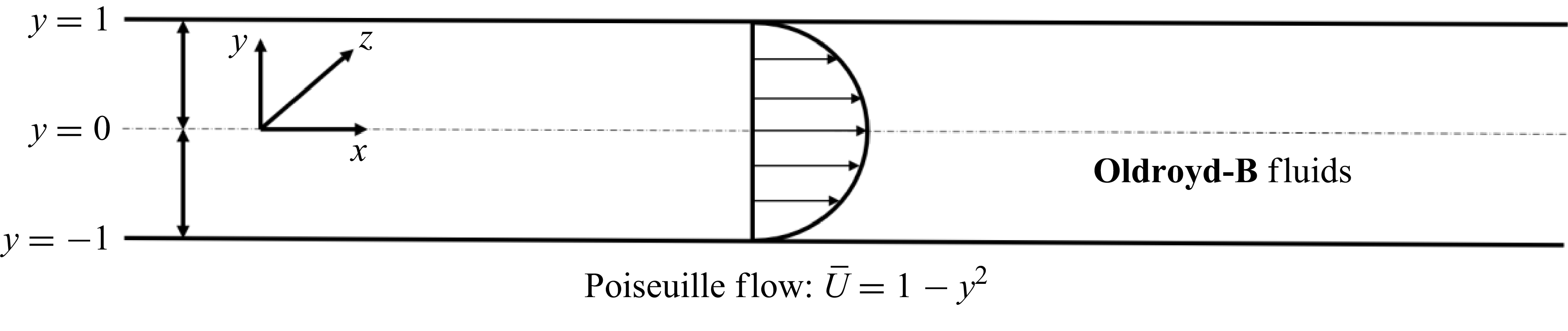
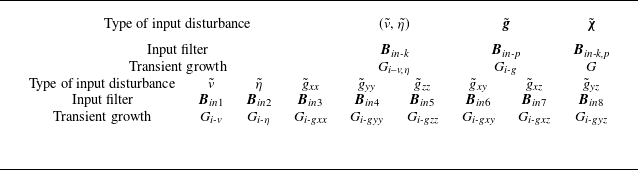
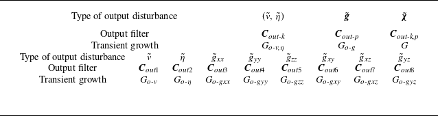
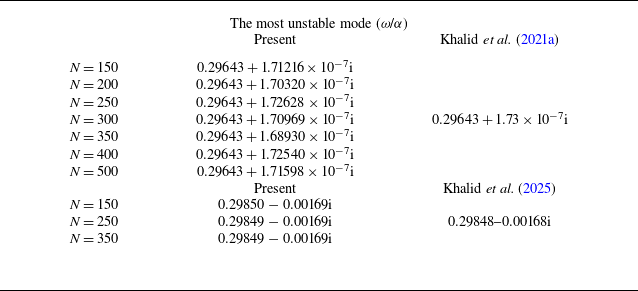


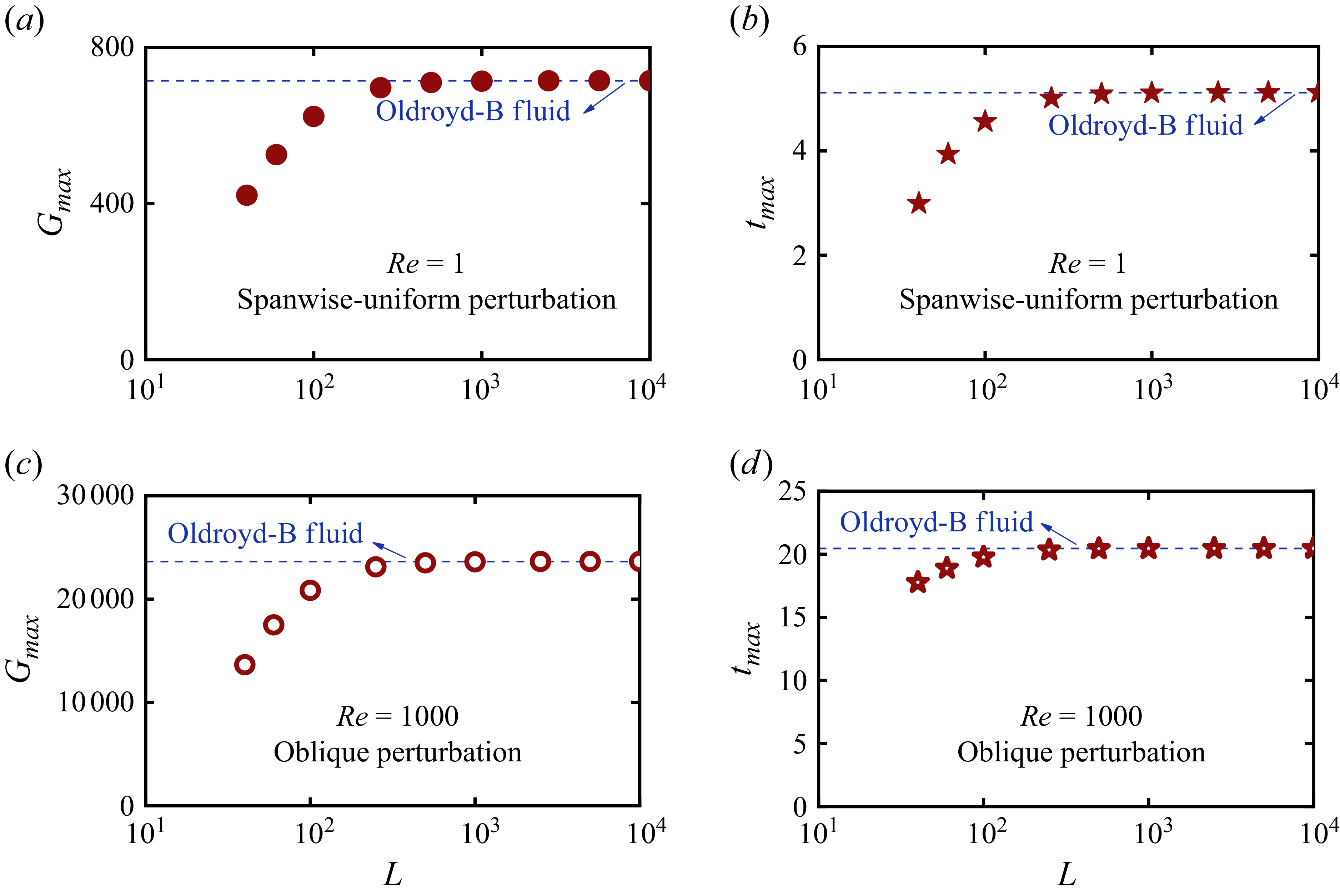

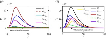


 g~
 u~
 c~


