



1. Introduction
Many natural and industrial systems feature turbulent flows of immiscible fluids. Examples include liquid fuel injection (Lefebvre & McDonell Reference Lefebvre and McDonell2017), breaking waves (Deike Reference Deike2022) and the food industry (Håkansson & Brandt Reference Håkansson and Brandt2022), among others. When evolving in a turbulent environment, the fluid parcels delimited by the interface deform and may fragment and/or coalesce (Risso & Fabre Reference Risso and Fabre1998; Vela-Martín & Avila Reference Vela-Martín and Avila2021; Ni Reference Ni2024; Zednikova et al. Reference Zednikova, Stanovsky and Orvalho2025). Historically, this problem was tackled starting from the ideal case of a unique element interacting with homogeneous isotropic turbulence at large Reynolds number, now referred to as the Kolmogorov–Hinze framework (Kolmogorov Reference Kolmogorov1949; Hinze Reference Hinze1955), and that suggests that breakup occurs when the surrounding fluid turbulent stresses at the scale of the element are larger than the surface tension cohesive forces.
This condition for breakup is associated with a specific scale, i.e, the Kolmogorov–Hinze scale: only drops larger than or similar to this scale can break. Whereas the breakup of a drop in high-turbulence-intensity flows shows violent modes (multifragment, bag, catastrophic), it reduces to a binary mechanism where a drop divides into two when the drop and Kolmogorov–Hinze scales are of the same order of magnitude.
As similarly observed for bubbles (Risso & Fabre Reference Risso and Fabre1998; Ni Reference Ni2024), the drop oscillates in this case and deforms under the action of turbulent pressure forces as well as capillary forces (Roa et al. Reference Roa, Renoult, Dumouchel and Brändle de Motta2023), sometimes taking the form of two blobs connected by a liquid bridge, as shown in figure 1(a). This bridge may either retract, leading to a recovering of the drop, or accentuate, leading to the binary breakup of the drop (Qi et al. Reference Qi, Xu, Tan, Zhong, Wu and Ni2024). Thus, the shape shown in figure 1(a) is not a sufficient condition for observing a binary rupture mechanism and the breakup condition is associated with a critical deformation state (CDS) characterising a drop deformation beyond which breakup is ineluctable.
Several CDS criteria have been proposed in the literature, such as, for instance, in Deberne et al. (Reference Deberne, Chéron, Poux and Brändle de Motta2024), where seven different criteria were presented (see their table 2). Defined by geometric or morphological characteristics (e.g. bounding box length, total surface area or average curvature), these criteria were computed statistically from a database, and a threshold distinguishing between stable and unstable drops was computed. Similar methodology was used for predicting breakup in droplets and bubbles (Qian et al. Reference Qian, McLaughlin, Sankaranarayanan, Sundaresan and Kontomaris2006; Perlekar et al. Reference Perlekar, Biferale, Sbragaglia, Srivastava and Toschi2012; Lalanne et al. Reference Lalanne, Masbernat and Risso2019).
(a) Realistic droplet from the database moments before breakup. (b) Ideal model proposed by Xing et al. (Reference Xing, Wang, Guo and Wang2015), where
 $R_1$
(blue) and
 $R_2$
(red) indicate the radii of the biggest and smallest spheres, respectively, and
 $R_3$
(orange) corresponds to the radius of the cylinder connecting them.

After considering Xing et al. (Reference Xing, Wang, Guo and Wang2015), Håkansson et al. (Reference Håkansson, Crialesi-Esposito, Nilsson and Brandt2022) suggested a CDS criterion for cases where the drop adopts a shape that can be modelled by two spheres connected by a cylinder, as portrayed in figure 1(b). The Laplace pressure in the cylinder is given by
 $P_{c} = P_0 + \sigma /R_{3}$
and the pressure in the lobes by
 $P_{s_1} = P_0 + 2\sigma /R_{1}$
and
 $P_{s_2} = P_0 + 2\sigma /R_{2}$
, where
 $R_1$
,
 $R_2$
and
 $R_3$
are the radii of the two spheres and the cylinder, respectively, and
 $\sigma$
is the surface tension. The pressure
 $P_0$
stands for the pressure of the surrounding fluid, which is assumed to be constant. The CDS criterion states that if the pressure at the cylinder is greater than the pressure in the smallest sphere, i.e.
 $P_{c} \gt P_{s_2}$
, the liquid in the neck will discharge towards the blobs until they split up. However, if
 $P_{c} \lt P_{s_2}$
, the neck is resupplied by the blobs and breakup does not occur. Håkansson et al. (Reference Håkansson, Crialesi-Esposito, Nilsson and Brandt2022) defined this critically deformed state as a state from which breakup will follow deterministically, even if no further external stresses would act on the drop. This suggests that the dynamics of the binary breakup results from capillary efforts only. Here, we aim at addressing the deterministic nature of the geometric CDS introduced by Håkansson et al. (Reference Håkansson, Crialesi-Esposito, Nilsson and Brandt2022) in more detail, more specifically questioning the CDS ‘criticality’ depending on the features of the external flow field.
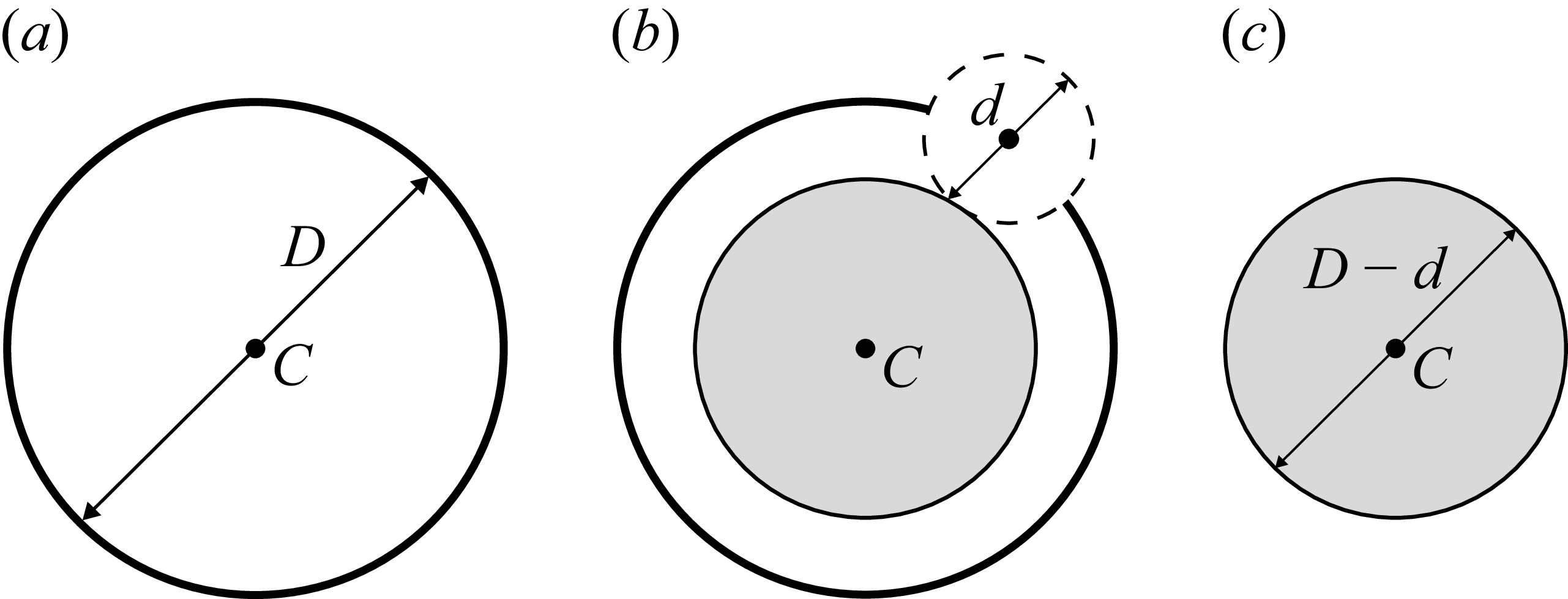
Erosion operation at scale
 $d$
of a sphere of diameter
 $D$
and centre
 $C$
. (a) Initial sphere, (b) erosion operation at scale
 $d$
, (c) the resulting eroded body is a sphere of diameter
 $D {-} d$
and centre
 $C$
.

This study proposes to interpret the results of numerical simulations of droplets immersed in homogeneous and isotropic turbulence using the CDS criterion introduced by Håkansson et al. (Reference Håkansson, Crialesi-Esposito, Nilsson and Brandt2022). Determining the
 $R_{1}$
,
 $R_{2}$
and
 $R_{3}$
scales used in the CDS is not straightforward for droplets with realistic deformation such as the one shown in figure 1(a). A scale-by-scale shape analysis of the droplets is applied to overcome this difficulty. The droplet shapes are described by their Euler characteristic as well as those of their parallel or eroded systems (Dumouchel et al. Reference Dumouchel, Thiesset and Ménard2022), which are obtained from a series of erosion operations as illustrated in figure 2 and explained hereafter. This tool is nicely tailored for identifying the typical deformation scales of the fluid parcels and their evolution in time. In particular, the regions associated with contraction (bottlenecks) and accumulation (blobs) patterns can readily be highlighted, thereby allowing the aforementioned CDS criterion to be tested on realistic droplet shapes. Furthermore, the deterministic nature of the breakup event at the CDS is explored by extending the simulations to theoretical cases with modified turbulent conditions. Finally, additional simulations illustrating the influence of droplet shape and Ohnesorge number on the intrinsic capillary instability are presented. This raises the question of whether a more comprehensive description of droplet morphology should be considered.
2. Description of the drop deformation
The technique chosen in the present work to describe the drop deformation is taken from a previous work (Dumouchel et al. Reference Dumouchel, Thiesset and Ménard2022). First, the drop is associated with a series of parallel systems obtained from a series of erosion operations. Second, the drop and its parallel systems are associated with quantities issued from integral geometry. The dependence of these quantities on the parallel systems offers a description of the drop deformation.
Commonly used in image analysis, an erosion operation consists of removing the part of the body under consideration covered by a sphere of diameter
 $d$
that has been slid over the entire interface of the body while keeping the centre of the sphere on this interface. The diameter
 $d$
of the eroding sphere is referred to hereafter as the scale. Figure 2 shows the example of the erosion at scale
 $d$
(figure 2
b) of a sphere of diameter
 $D$
and centre
 $C$
(figure 2
a). The resulting eroded body is a sphere of diameter
 $D {-} d$
and centre
 $C$
(figure 2
c). All normals of the eroded system being also normals of the initial system, the two systems are therefore said to be parallel to each other.
In an
 $n$
-dimensional space,
 $n+1$
integral quantities are required to provide a complete description of the shape of any body (Mecke Reference Mecke2002). Known as the Minkowski functionals (MFs), these quantities reflect the integration of local characteristics across the entire system. For example, the MFs for
 $n=3$
correspond to the volume, the surface, the surface integrated mean curvature and the surface integrated Gaussian curvature. The present analysis considers only the latter, which is defined as
 \begin{align} G = \int _{S} \kappa _1 \kappa _2 \,\text{d}S, \end{align}
where
 $S$
designates the body surface,
 $\text{d}S$
is an elementary surface element and
 $\kappa _1$
and
 $\kappa _2$
are the two principal curvature components at each point of the surface. By virtue of the Gauss–Bonnet theorem, for a closed surface, the surface integrated Gaussian curvature
 $G$
is related to the Euler characteristic
 $\chi$
by
 \begin{align} G = 2\pi \chi . \end{align}
The topological invariant
 $\chi$
depends only on the topology of the body under consideration, regardless of the way it is bent. For instance,
 $\chi = 2$
for a sphere as well as for any other body homeomorphic to a sphere, e.g. a spheroid. The characteristic
 $G$
(and therefore
 $\chi$
) is additive: its value for a system made of several bodies is the sum of the values of each body. Thus, the Euler characteristic of
 $N$
spheroids is equal to
 $2N$
.
In the present analysis, a drop is described at each instant by the function
 $G(d)$
(or
 $\chi (d)$
), i.e. the surface integrated of the Gaussian curvature (or the Euler characteristic) of the parallel systems of the drop according to erosion scale
 $d$
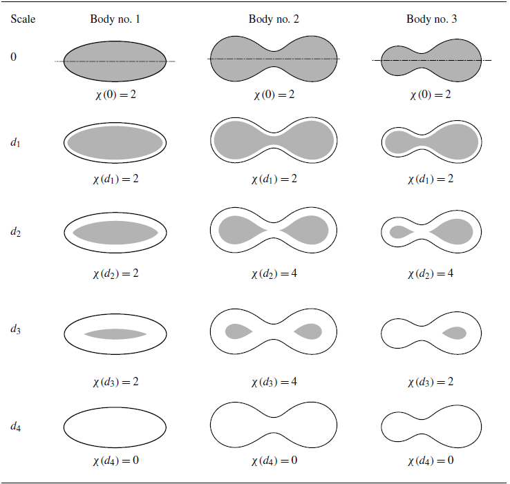
. This approach is illustrated in table 1 for three bodies (body no. 1, no. 2 and no. 3) exhibiting an axial symmetry whose axis is the dashed line drawn in the first row. Each row reports the eroded system of each body for the scale indicated in the first column as well as the corresponding value of the Euler characteristic
 $\chi (d)$
. The black continuous lines in table 1 delimit the initial bodies. The grey areas delimit the eroded bodies.
Examples of body erosions and corresponding values of the Euler characteristic of the eroded body. Black lines delimit the body, the dashed line shows the symmetry axis and the grey areas delimit the eroded or parallel system for the scale indicated in first column.

Table 1. Long description
Panel A: Body no. 1. The diagram shows the erosion of body no. 1 at different scales. Each row represents a different scale, with the body outlined in black and the eroded area shaded in grey. The Euler characteristic values are provided for each scale. Panel B: Body no. 2. The diagram shows the erosion of body no. 2 at different scales. Each row represents a different scale, with the body outlined in black and the eroded area shaded in grey. The Euler characteristic values are provided for each scale. Panel C: Body no. 3. The diagram shows the erosion of body no. 3 at different scales. Each row represents a different scale, with the body outlined in black and the eroded area shaded in grey. The Euler characteristic values are provided for each scale.
When the scale is equal to zero (first row,
 $d = 0$
), the initial and eroded bodies coincide. Since the three bodies in table 1 are each homeomorphic to a single sphere,
 $\chi (0) = 2$
. Note that the drops of interest in this work will be always homeomorphic to a sphere such that
 $\chi (0) = 2$
before breakup. For small scales (second row,
 $d = d_{1}$
), the eroded systems remain homeomorphic to a sphere and their Euler characteristics are unchanged;
 $\chi (d_{1}) = 2$
. There exist larger scales (third row,
 $d = d_{2}$
), for which the eroded system of bodies no. 2 and no. 3 shows two disconnected parts and has therefore a double Euler characteristic,
 $\chi (d_{2}) = 4$
. This does not occur for body no. 1. There exist even larger scales (fourth row,
 $d = d_{3}$
), for which one of the two parts of the eroded system might disappear if the initial sizes of the two parts are different. This is the case for body n
 $\textrm{o}.$
3, whose Euler characteristic of the eroded system is reduced,
 $\chi (d_{3}) = 2$
. Finally, at very large scales (fifth row,
 $d = d_{4}$
), the bodies are totally eroded and their eroded system Euler characteristics are equal to
 $0$
.
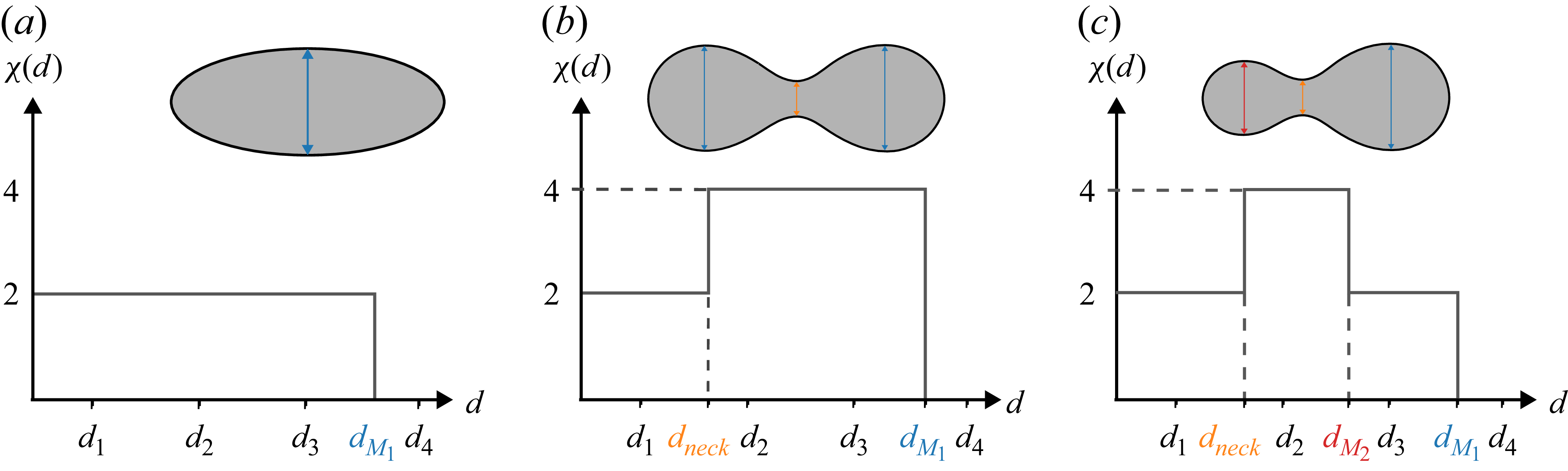
For the three bodies considered in table 1, the functions
 $\chi (d)$
are schematised in figure 3, where the scales
 $d_1$
,
 $d_2$
,
 $d_3$
and
 $d_4$
are also positioned. We note that the jumps of
 $\chi (d)$
always occur at characteristic scales of the body. An increase of
 $\chi (d)$
at a scale occurs when the erosion operation carried out at this scale produces a disconnected eroded system. This scale is therefore representative of a contraction size of the initial system. This scale is named
 $d_{\textit{neck}}$
in figure 3 and is indicated in orange. A decrease of
 $\chi (d)$
at a scale occurs when the erosion operation carried out at this scale causes all or part of the body to disappear. For body no. 2 (figure 3
b), this occurs only once at scale
 $d_{M_1}$
, indicated in blue in the figure, and that corresponds to the size of the bulges on each side of the contraction. For body no. 3 (figure 3
c), a decrease of
 $\chi (d)$
is observed twice since the bulges on each side of the contraction have a different size. In this case,
 $\chi (d)$
makes it possible to identify the scale of each bulge, i.e.
 $d_{M_1}$
the last decrease of
 $\chi (d)$
and
 $d_{M_2}$
the first decrease of
 $\chi (d)$
. These scales are represented in blue and red, respectively, in figure 3(c). For body no. 1, the only scale that emerges is scale
 $d_{M_1}$
.
Evolution of the Euler characteristic
 $\chi (d)$
of the eroded body as a function of the scale of erosion
 $d$
for the bodies of table 1. Identification of the scales of interest in the present analysis. (a) Body n
 $\textrm{o}.$
1. (b) Body n
 $\textrm{o}.$
2. (c) Body n
 $\textrm{o}.$
3.

The work focuses on the breakup of the drops. When such an event occurs, the drop deformation shows at least one neck. The scale for which
 $\chi (d)$
increases from
 $2$
to
 $4$
, called
 $d_{\textit{neck}}$
, refers to this situation. More generally, an increase of
 $\chi (d)$
may also occur when the drop shows a flattened zone, but such a deformation does not signal a breakup. Therefore, the
 $d_{\textit{neck}}$
scale of interest characterises a rather cylindrical liquid bridge to which we can associate a Laplace pressure defined by
 \begin{align} P_{\textit{neck}} = P_{0} + 2\frac {\sigma }{d_{\textit{neck}}}. \end{align}
Considering that the swollen parts of the deformed drop are close to spheres, the Laplace pressure associated with the scales
 $d_{M_1}$
and
 $d_{M_2}$
is defined by
 \begin{align} P_{M_{i}} = P_{0} + 4\frac {\sigma }{d_{M_{i}}},\quad \text{for}\quad i=1,2. \end{align}
The objective is to build a condition of rupture by comparing the Laplace pressure
 $P_{\textit{neck}}$
,
 $P_{M_1}$
and
 $P_{M_2}$
.
Here, the eroded system at scale
 $d$
is obtained directly from numerical data using the signed-distance function with positive values corresponding to the disperse phase. The computation of the Gaussian curvature is carried out using the routines already described by Di Battista et al. (Reference Di Battista, Bermejo-Moreno, Ménard, de Chaisemartin and Massot2019), Essadki et al. (Reference Essadki, Drui, de Chaisemartin, Larat, Ménard and Massot2019) and Dumouchel et al. (Reference Dumouchel, Thiesset and Ménard2022).
Note that our methodology is not limited to codes that explicitly solve an evolution equation for the distance function. When volume-of-fluid (VoF) or diffuse interface methods are used, the distance function can be postcomputed using, e.g., a marching-cubes algorithm. The Euler characteristics can also be obtained using simple object labelling and counting methods, albeit the eroded systems remain homeomorphic to spheres. Although not systematically observed, there are possible cases where the deformed droplet is flattened so that the eroded system becomes homeomorphic to a torus, with
 $\chi =0$
. The computation of
 $G$
was preferred as it is more robust and provides an accurate topological representation of the system.
In summary, to compute the CDS in a simple way, it is necessary to compute the distance function by applying a marching-cubes algorithm. Then, from each eroded system (defined as the shape given by an isovalue of the distance function), the number of elements can be computed with a labelling algorithm. Then the change in the number of elements provides the lengths
 $d_{\textit{neck}}$
(first length where there is more than one element) and
 $d_{M_2}$
(length where there are one or fewer elements). By computing
 $P_{\textit{neck}}$
and
 $P_{M_2}$
with (2.3) and (2.4), respectively, the criteria can be verified by checking if
 $P_{\textit{neck}} \gt P_{M_2}$
or not.
3. Numerical methodology
3.1. ARCHER solver
The numerical database presented here has been obtained using the high-performance computing code ARCHER developed at CORIA laboratory (Ménard et al. Reference Ménard, Tanguy and Berlemont2007). It solves on a staggered Cartesian mesh the one-fluid formulation of the incompressible Navier–Stokes equations.
For transporting the interface, a coupled level-set (signed-distance) and volume-of-fluid (CLSVOF) method is used. The level-set function accurately describes the geometric features of the interface (its normal and curvature) while the VoF function ensures mass conservation.
The convective term is written in the conservative form and solved using the improved Rudman’s technique (Rudman Reference Rudman1998; Vaudor et al. Reference Vaudor, Ménard, Aniszewski, Doring and Berlemont2017). The viscous term is computed following the scheme presented in the work of Sussman et al. (Reference Sussman, Smith, Hussaini, Ohta and Zhi-Wei2007). To ensure the incompressibility of the velocity field, a Poisson step is solved using a multi grid preconditioned conjugate gradient algorithm (MGCG) (Zhang Reference Zhang1996) coupled with a ghost fluid method (Fedkiw et al. Reference Fedkiw, Aslam, Merriman and Osher1999). The ARCHER code has been used to investigate primary atomisation (Lebas et al. Reference Lebas, Menard, Beau, Berlemont and Demoulin2009) and secondary atomisation under turbulent conditions (Duret et al. Reference Duret, Luret, Reveillon, Ménard, Berlemont and Demoulin2012).
The use of the level-set function to describe the interface makes it straightforward to compute the MFs of the system. Indeed, this function is nothing but the implicit definition for the set of parallel systems at a distance
 $d$
. The Gaussian curvatures
 $G(d)$
for each level set
 $d$
are computed using the method of Essadki et al. (Reference Essadki, Drui, de Chaisemartin, Larat, Ménard and Massot2019) and Di Battista et al. (Reference Di Battista, Bermejo-Moreno, Ménard, de Chaisemartin and Massot2019), which is implemented in a specific postprocessing submodule of the ARCHER code. In practice, the isoelements are computed at a fixed step distance; here, 150 isoelements are computed over the initial droplet radius. This step gives the distance between the parallel elements. This means that the computation of the MFs does not provide smooth signals like the ones presented in the work of Dumouchel et al. (Reference Dumouchel, Thiesset and Ménard2022), where the level sets are computed for ideal and well-refined shapes.
3.2. Database of droplets in turbulence
As a part of previous studies (Roa et al. Reference Roa, Renoult, Dumouchel and Brändle de Motta2023; Deberne et al. Reference Deberne, Chéron, Poux and Brändle de Motta2024), a database of independent droplets immersed in a homogeneous and isotropic turbulent background flow was generated. These previous studies consider the oscillations of the droplet, the breakup and their lifetime. The current work focuses on the later moments before the breakup using the same database. This database was created by performing multiple realisations of the same physical configuration, with the viscous and density ratios, as well as the turbulent Reynolds and Weber numbers, kept constant. The numerical simulation was performed over a
 $64^3$
grid, providing a sufficient resolution to capture the interactions between the droplets and the surrounding turbulent flow. To maintain the turbulent characteristics at statistically steady state, a linear forcing adapted to two-phase flows has been applied (Rosales & Meneveau Reference Rosales and Meneveau2005; Duret et al. Reference Duret, Luret, Reveillon, Ménard, Berlemont and Demoulin2012). The ratio between the initial droplet radius
 $R$
and domain size
 $L$
is
 $R/L = 0.233$
. The Reynolds number is defined as
 $ \textit{Re}_\lambda = u'^2\sqrt { 5 \rho _{2} / (3\mu _{2} \epsilon ) } \simeq 40$
, where
 $u'^2$
is twice the averaged turbulent kinetic energy and
 $\epsilon$
is the kinetic energy dissipation rate. The subscripts
 $1$
and
 $2$
indicate the dispersed and continuous phase, respectively. The turbulent timescale is
 ${ ( (2 R)^2 / \epsilon )}^{1/3}=2.3\,t_{c}$
, where
 $t_{c} = \sqrt {\rho _{1} R^{3}/\sigma }$
is the capillary timescale, with
 $\rho _1$
the density of the dispersed phase. The Weber number, defined as
 $ \textit{We} = \rho _{1} u'^{2} 2 R/\sigma$
, of
 $0.9$
, and an Ohnesorge number
 $ (Oh = \mu _{1}/\sqrt {\sigma \rho _{1}R} )$
of
 $0.00465$
were considered. This Weber number was set to ensure the droplet would deform before experiencing breakup. The viscosity ratio (
 $\mu _{2}/\mu _{1}$
) as well as density ratio (
 $\rho _{2}/\rho _{1}$
) are set to unity. For the results presented here, 181 breaking droplets were analysed. For more information on the database generation, the reader is advised to refer to the work by Deberne et al. (Reference Deberne, Chéron, Poux and Brändle de Motta2024).
Two reduced-size databases were generated with finer grids to assess mesh convergence. These databases contain (a) 28 droplets with double the grid resolution per axis (
 $128^3$
) and (b) 11 droplets with four times the grid resolution per axis (
 $256^3$
). These two databases share the same physical parameters as the reference database presented in the paragraph just above. The statistical study of these databases is given in Appendix A, confirming that the simulations used to reproduce results presented in § 4 are resolved enough.
Two other datasets are also generated in order to prove the limits of the current study. From the refined setup (the
 $128^3$
mesh), a set of droplets with
 $ \textit{Re}_{\lambda } = 80$
is simulated, i.e. double the original
 $ \textit{Re}_{\lambda }$
. From the original database of droplets (the
 $64^3$
mesh), the Weber number was expanded to three different Weber values. For
 $ \textit{We} =1.35, 1.8$
, we observed a similar trend to the results of our original database, as shown in Appendix B. It has been observed that for
 $ \textit{We}=4.5$
, the breakup is no longer binary and therefore, the droplets are not considered in this study.
4. Results
4.1. Scale-by-scale analysis of drop deformation and breakup
We first present the time evolution of the scales
 $d_{M_1}$
,
 $d_{M_2}$
and
 $d_{\textit{neck}}$
defined in § 2 for one arbitrary chosen drop of the database. Qualitatively similar observations were made for the other realisations. Results are depicted in figure 4 where the time axis spans from the initial spherical state of the drop to the breakup event and is normalised by the capillary timescale. The first response of the droplet to the turbulent surrounding is to depart from its spherical state, which manifests as the decrease of
 $d_{M_1}$
within the first
 $2\,t_{c}$
. After that, the variation of the scales illustrates the drop deformation and oscillation resulting from the stresses of the surrounding turbulent flow (Roa et al. Reference Roa, Renoult, Dumouchel and Brändle de Motta2023).
Time evolution of the scales
 $d_{M_1}$
(blue),
 $d_{M_2}$
(red) and
 $d_{\textit{neck}}$
(orange) for a breaking droplet (see evolution in supplementary movie is available at https://doi.org/10.1017/jfm.2026.11953). The navy, purple and black vertical dashed lines indicate the start of the last neck formation, the critical state and the breakup event, respectively. Similar figures for droplets generated with refined meshes are presented in figure 9 of Appendix A.

As discussed before, the fragmentation event is supposed to be triggered by the formation of two liquid lobes connected by a cylindrical liquid bridge. As explained in figure 3, the presence and size of such a bridge is characterised by the instances in which
 $d_{\textit{neck}}$
can be identified. One interesting finding of this study is that these events can be found multiple times during the drop lifetime. Indeed, figure 4 reveals that a neck (as per the definition of § 2) begins to form, for example at
 $t \approx 12\,t_{c}$
, and is followed by a return to a state without neck at
 $t \approx 15.5\,t_{c}$
. At a later time of
 $t \approx 19\,t_{c}$
, another neck forms, but this time it leads to fragmentation of the drop at
 $t \approx 23\,t_{c}$
. Shortly before the breakup event (
 $t \approx 22\,t_{c}$
), the scale
 $d_{\textit{neck}}$
promptly drops to zero. The time evolution of the blob scales
 $d_{M_1}$
and
 $d_{M_2}$
presented in figure 4 reveals that as a neck forms,
 $d_{M_1}$
and
 $d_{M_2}$
are close to each other. When the liquid bridge thins, these scales may depart from each other, indicating that the two blobs may differ in size and shape.
It should be remembered from figure 4 that the formation of a neck does not constitute an indicator of an upcoming breakup. In what follows, the CDS criterion proposed by Håkansson et al. (Reference Håkansson, Crialesi-Esposito, Nilsson and Brandt2022) is applied.
4.2. The CDS criterion
The CDS criterion is constructed by linking the scales
 $d_{M_1}$
,
 $d_{M_2}$
and
 $d_{\textit{neck}}$
to the pressure distributions in the drop, denoted
 $P_{M_1}$
,
 $P_{M_2}$
and
 $P_{\textit{neck}}$
, as presented in § 2 and plotted in figure 5(a) as a function of
 $(t - t_{\textit{breakup}})$
and where each coloured line corresponds to the ensemble average over the whole database. The filled regions correspond to the root-mean-square error (RMSE). We observe that the dynamics of deformation and breakup are similar for all drops of the database. The pressures slightly vary until the drops are deformed strongly enough that the pressure at the neck becomes higher than the one at the smallest lobe, i.e.
 $P_{\textit{neck}} \geqslant P_{M_2}$
. The time at which this threshold is exceeded is defined as
 $t_{\textit{critical}}$
. Beyond this threshold, the neck rapidly thins, and the pressure
 $P_{\textit{neck}}$
promptly increases, thereby discharging the liquid from the neck to the bulbs. All the drops of the database experience break up when passing this point. Therefore, the present analysis provides unprecedented support in favour of the CDS proposed by Håkansson et al. (Reference Håkansson, Crialesi-Esposito, Nilsson and Brandt2022).
(a) Representation of the Laplace pressures obtained from the scales
 $d_{M_1}$
,
 $d_{M_2}$
and
 $d_{\textit{neck}}$
for all droplets of the database. The averaged values in the interval
 $(t_{\textit{breakup}} - t) \gt -10\,t_{c}$
are represented by the blue, red and orange lines. The RMSE over the complete database is represented by the filled regions in their respective colours. The vertical purple dashed line is the average critical time
 $\langle t_{\textit{critical}} \rangle$
. The same results with finer grids are presented in figure 8 of Appendix A. (b) The distribution of the excursion time for the droplets in the database. (c) The distribution of breakup time for the droplets in the database (light grey) and for the droplets starting from the CDS and initially quiescent flow (dark grey, see definition of case Q in § 4.3).

Figure 5. Long description
Panel A: A line graph shows the Laplace pressures obtained from different scales for all droplets in the database. The x-axis represents normalized time (t - t_breakup)/t_c, and the y-axis represents the Laplace pressure P_L. The graph includes multiple lines representing averaged values for different scales: blue for d_M1, red for d_M2, and orange for d_neck. The filled regions around these lines indicate the root mean square error (RMSE) over the complete database. A vertical purple dashed line marks the average critical time t_critical. Panel B: A histogram displays the distribution of the excursion time for the droplets in the database. The x-axis represents normalized excursion time (t_breakup - t_excursion)/t_c, and the y-axis represents the probability density function (p.d.f.). Panel C: Another histogram shows the distribution of breakup time for the droplets in the database. The x-axis represents normalized breakup time (t_breakup - t_critical)/t_c, and the y-axis represents the probability density function (p.d.f.). The light grey bars represent orginal database, while the dark grey bars represent droplets starting from the critical deformation state (CDS) and initially quiescent flow.
We introduce the excursion time, denoted
 $t_{\textit{excursion}}$
, the time at which a neck leading to breakup is formed. This time is illustrated in figure 4 by the cyan vertical line. The latter is determined for the whole database and its probability density function is plotted in figure 5(b). The time between the formation of the neck and the fragmentation varies greatly. It can last for
 $20\,t_{c}$
but can be as short as
 $4\,t_{c}$
. The average is rather about
 $9\,t_{c}$
. Such large temporal fluctuations between neck formation and droplet breakup indicate that, prior to the CDS, the competition between capillary restoring force and external turbulent perturbations can persist over a relatively long period before reaching the CDS.
Temporal evolution of the ratio
 $d_{\textit{neck}}/2R$
from the critical time. The graphs (a) (b) and (c) show the behaviour of three droplets with different shapes at
 $t_{\textit{critical}}$
. These droplets are depicted in each graph. For each droplet, the four cases are presented as case FT (dashed line), case DT (dashed–dotted line), case EQ (dotted line) and case Q (continuous line).

The probability density function of the time between the critical state and breakup time for the whole database is presented by the light-grey histogram in figure 5(c). This histogram, which is of course narrower than the one in figure 5(b), shows highly variable rupture times, ranging from
 $0.5$
to
 $2$
times the capillary time
 $t_c$
. By definition, the capillary time
 $t_c$
is characteristic of the effects of capillary forces at the droplet scale, i.e. stabilising effects (i.e. opposing rupture). The range of break times shown in figure 5(c) suggests a variability in the breakup dynamics during the later stages before breakup. The additional simulations presented in §§ 4.3 and 4.4 provide insights into this issue.
4.3. Influence of the turbulent environment on the rupture dynamics
This section attempts to identify the possible influence of turbulence on the breakup dynamics represented by the temporal evolution of the ratio
 $d_{\textit{neck}}/2R$
from the critical time
 $t_{\textit{critical}}$
to the breakup time. Partly inspired by the work of Håkansson et al. (Reference Håkansson, Crialesi-Esposito, Nilsson and Brandt2022), supplementary simulations have been conducted with different turbulent conditions but similar initial droplet shape. Including the initial simulations, four simulation cases are now available:
-
(i) Case FT (forced turbulence): initial simulations in which the surrounding turbulence forcing is maintained over time.
-
(ii) Case DT (decaying turbulence): at
 $t = t_{\textit{critical}}$
, the turbulence forcing is set to zero.
-
(iii) Case EQ (external quiescent): at
$t = t_{\textit{critical}}$
, the surrounding velocity field is set to zero while keeping the internal velocity field free to decay. -
(iv) Case Q (quiescent): at
$t = t_{\textit{critical}}$
, all velocity fields (inside and outside the droplets) are reset to zero.


The results of these simulations are shown in figure 6 for three droplets whose shapes at
 $t = t_{\textit{critical}}$
, shown in each graph, are different. Indeed, it is important to keep in mind that even if droplets satisfy the CDS, they might have different shapes at
 $t_{\textit{critical}}$
. The Ohnesorge number is equal to
 $0.0046$
and the line texture in figure 6 differentiates the simulation cases: dashed line (case FT), dashed–dotted line (case DT), dotted line (case EQ) and continuous line (case Q).
The simulations report different behaviours for the three droplets. The results of the initial simulations (case FT) display very similar rupture dynamics for the drops shown in figures 6(a) and 6(b) with a breakup time of the order of
 $0.6\,t_c$
for both of them. The drop in figure 6(c) reports a longer breakup time of the order of
 $1.1\,t_{c}$
Note that these breakup times lie on either side of the peak of the histogram (figure 5
c). Simulations of case DT show that a decaying turbulence from
 $t_{\textit{critical}}$
does not alter the breakup dynamics for the droplets in figures 6(a) and 6(b), while the breakup of the third droplet is slightly delayed (figure 6
c). Although the impact of decaying turbulence remains minor for this latter drop, it is evidenced by an increase of the breakup time from
 $1.1\,t_c$
to
 $1.2\,t_c$
. The difference between the cases with decaying and forced turbulence (cases DT and FT) is small since the time for the turbulence to decay is large compared to
 $t_c$
. Here, the turbulent turnover time is
 $u'^2/\epsilon =3.7\,t_c$
. The difference between forced and decaying is only visible when the breakup time begins comparable to
 $t_c$
.
The third set of simulations (case EQ), which removes the surrounding turbulence at time
 $t_{\textit{critical}}$
, yields different results for the three droplets. The droplet in figure 6(a) appears unaffected by this change, and its breakup dynamics remain unchanged compared to the previous simulations. The droplet in figure 6(b) exhibits slower breakup dynamics in this case compared to the previous one. Finally, the absence of external turbulent stresses on the third droplet (figure 6
c) prevents it from breaking.
The fourth simulation case (case Q) imposes zero velocity field inside and outside the droplet at
 $t_{\textit{critical}}$
. These simulations provide insight into the ability of capillary forces alone to trigger a binary rupture. For the droplet shown in figure 6(a), we note that the temporal decay of
 $d_{\textit{neck}}/2R$
is slightly delayed but remains rather parallel to those found for the previous simulation cases. Therefore, the figure 6(a) droplet has a rupture dynamic insensitive to the turbulence. For this droplet, the rupture dynamic is purely capillary and can be qualified as intrinsic or deterministic instability, i.e. it depends on nothing else but the shape of the droplet. The time lag observed for case Q illustrates the delay required by the capillary efforts to set in motion the droplet internal flow.
The droplet of figure 6(b) reports for case Q a very different rupture dynamic compared to the previous cases. When the binary rupture is controlled by the capillary efforts only, the breakup time is almost doubled. For this droplet, we understand that whereas the turbulence of the surrounding environment is not required to trigger the binary breakup event, it contributes to its acceleration. Contrary to the previous droplet, the binary breakup of the figure 6(b) droplet in a turbulent environment is not a deterministic or intrinsic instability.
Finally, as expected after the case EQ simulation, the figure 6(c) droplet does not break when left to the action of capillary forces alone (case Q). The simulation series for this droplet clearly demonstrates the essential need for external stress (the turbulence in the present work) for the binary breakup to take place. Thus, based on the results in figure 6, it is clear that the turbulence of the external environment has a negligible, contributing or essential influence on the binary breakup of the droplet after the CDS is reached.
Simulations of case Q, performed on all droplets in the database, showed that breakage is still observed in
 $81\,\%$
of the droplets. Thus, droplets of the type shown in figure 6(c) account for
 $19\,\,\%$
of the entries in the database and are therefore not negligible. The different behaviours shown in figure 6 are related to the shape of the droplets at time
 $t_{\textit{critical}}$
. In figure 5(c), the distribution of breakup times of the cases FT and Q are compared. The shift to larger times for the quiescent initial flow, observed in droplet 6(b), is then statistically observed. There are no breakup times smaller than
 $0.82\,t_c$
for the quiescent flow, and the average breakup time passes from
 $0.94\,t_c$
for the forced turbulent case to
 $1.19\,t_c$
for the quiescent case.
The binary breakup of a droplet results from the competition of internal flows with opposite effects. For the case of stretched ligament relaxation, Tong & Wang (Reference Tong and Wang2007) demonstrated the existence of a recoiling flow from the blob toward the neck and an extension flow from the neck toward the blob. The recoiling flow opposes rupture, while the extension flow leads to rupture. They also observed that the dominance of one flow over the other is directly related to the shape of the blob, i.e. to the curvature distribution that characterises it. They also pointed out that according to the curvature distribution around the neck, the peak of pressure might be located next to the neck. It seems reasonable to assume that the droplets studied here contain similar flows and characteristics to those identified by Tong & Wang (Reference Tong and Wang2007). In consequence, the full curvature distribution along the interface of the droplets must be considered when predicting their rupture. As far as this study is concerned, we understand that even when the CDS criterion is met, some droplet shapes are not appropriate to generate capillary instability leading to binary breakup through capillary forces alone. To illustrate the importance of the droplet shape on the resulting capillary forces and their ability to trigger binary rupture, supplementary simulations with varying Ohnesorge number are presented in the last section.
Temporal evolution of the ratio
 $d_{\textit{neck}}/2R$
from the critical time. The graphs (a) (b) and (c) show the behaviour of the three droplets considered in figure 6 with different initial shapes at
 $t_{\textit{critical}}$
. These droplets are depicted in each graph considering initial quiescent flow. The black line corresponds to
 $ \textit{Oh} = 0.0046$
(the original database Ohnesorge). Lines of different colours correspond to several
 $ \textit{Oh}$
numbers. The dashed line in graph (b) corresponds to the slope
 $-0.1$
. The same droplets with finer grids are presented in figure 10 of Appendix A.

Figure 7. Long description
Three line graphs depict the temporal evolution of the ratio from the critical time for droplets with different initial shapes (panels A, B and C). A line graph shows the ratio d_neck/2R over time (t - t_critical)/tc for droplets. The x-axis is labeled (t - t_critical)/tc and the y-axis is labeled d_neck/2R. Multiple colored lines represent different Oh values.
4.4. Effect of drop shape and Ohnesorge number on capillary instability
In addition to the previous simulations, this section presents simulations for different Ohnesorge numbers of the droplet. The Ohnesorge number is the ratio of viscous force to capillary and inertia forces. These additional simulations are performed for case Q only, maintaining both ratios
 $\mu _2/\mu _1$
and
 $\rho _{2}/\rho _{1}$
equal to unity. The Ohnesorge number was varied up to factors
 $[0.28 {-} 12]$
of the initial value
 $0.0046$
. The variations also impact the value of the capillary time
 $t_{c}$
.
Figure 7 reports the results for the three droplets examined in figure 6. The continuous lines of different colours correspond to the results for the considered range of Ohnesorge numbers.
For the three droplets, figure 7 shows that the dynamics of
 $d_{\textit{neck}}/2R$
are not influenced by the Ohnesorge number when it is less than or equal to
 $0.0046$
. Above this value, several scenarios are observed. While all dynamics slow down when the Ohnesorge number is greater than
 $0.0046$
, the binary breakup is never compromised for the droplet in figure 7(a), whereas it is compromised for the drop in figure 7(b). For this droplet, the breakup is no longer observed when the Ohnesorge number is greater than or equal to
 $0.0186$
. As expected, the third droplet (figure 7
c) never reports a binary breakup for the simulation series reported in this section. As far as the influence of the Ohnesorge is concerned, the results of figure 7(b) indicate a compromised binary breakdown if the initial slope of
 $d_{\textit{neck}}/(2R)$
is of the order
 $-0.1$
(see dashed line). This limit should be generalised to different shapes and
 $ \textit{Oh}$
numbers through a more detailed study.
The results here show that there is a competition between different phenomena: viscosity, inertia and surface tension. The effect of these phenomena is negligible for small
 $ \textit{Oh}$
, and can have an effect in different ways for larger
 $ \textit{Oh}$
by delaying and even preventing the breakup. The study of the balance between these phenomena is out of the scope of the current work.
The results of figure 7 show that the intrinsic capillary instability leading to binary breakup is not solely dependent on the pressure at the neck and in the smallest blob but involves the whole shape of the droplet. These observations are consistent with the findings of Tong & Wang (Reference Tong and Wang2007), who showed, for example, that the pressure peak does not always coincide with the position of the neck. This once again highlights the need to consider the entire shape of the droplets when studying their binary breakup.
5. Conclusions
Using numerical simulations combined with an analysis based on the use of Euler characteristic of the droplet and of its parallel systems, this work demonstrates that the definition of the CDS proposed by Håkansson et al. (Reference Håkansson, Crialesi-Esposito, Nilsson and Brandt2022) that is expressed as
 $P_{\textit{neck}}\gt P_{M_2}$
is appropriate for identifying the point at which droplets in a turbulent environment evolve into a binary breakup. This was confirmed on 181 drops in a turbulent environment reporting a binary rupture. In addition to the simulations used in this analysis, Appendix B reports simulations for only a few drops at other Reynolds and Weber numbers for which the validity of the established CDS is confirmed.
The influences of the turbulence, of the fluid properties and of the drop shape at
 $t_{\textit{critical}}$
(time at which the CDS is satisfied) on the dynamics of the binary breakup mechanism, i.e. from the critical to the breakup times, were investigated. For that, taking inspiration from Håkansson et al. (Reference Håkansson, Crialesi-Esposito, Nilsson and Brandt2022), supplementary simulations were performed from
 $t_{\textit{critical}}$
to
 $t_{\textit{breakup}}$
. These simulations considered additional cases with a relaxing turbulence, with no turbulence in the surrounding environment and with no turbulence everywhere. Analysis of these additional simulations shows that, depending on the shape of the droplets at the critical time, the turbulence has a negligible, contributory or essential effect on the binary breakup event. For droplets whose binary breakup is not influenced by turbulence, the CDS captures the transition from turbulence-driven deformation to capillary-driven breakup for binary breakup events and the CDS is associated with an irreversible configuration in which the pressure distribution within the droplet drives liquid drainage from the neck towards the two bulbs, ultimately leading to fragmentation. The rupture here is due to intrinsic capillary instability.
For the droplets for which the turbulence contributes to the rupture dynamics, the CDS also points to a situation where the conditions for an intrinsic capillary instability are fulfilled but the observed rupture dynamics are not solely due to capillary since turbulence effects are significant and accelerate the rupture.
Finally, droplets for which the turbulence is essential to trigger the binary breakup are not in the appropriate conditions for an intrinsic capillary instability at
 $t_{\textit{critical}}$
. These droplets, which represent
 $19\,\%$
of the database, do not break when considering initially quiescent flow. Their breakup in the presence of turbulence is therefore not due to an intrinsic capillary instability.
In other words, our findings suggest that the term ‘critical’ in ‘critically deformed state’ should be moderated. It is reliable to anticipate binary breakup under sustained turbulent forcing (valid in all 181 cases). However, in the absence of external turbulent stresses, although it designates the onset of intrinsic capillary instability, it leads to rupture in just 81 % of cases.
The numerical simulations conducted as part of this study demonstrate that these different behaviours are partly related to the shape of the droplets at the moment the CDS is satisfied. The influence of fluid properties on the drop capillary instability, i.e. post-CDS, as estimated by simulations at different Ohnesorge numbers (the ratio of viscous forces to capillary and inertia forces), also appears to depend on the shape of the droplets at the moment the criterion is satisfied. Thus, while the CDS evaluated in this analysis is suitable for treating the case of binary droplet breakup in a turbulent environment, it is not a universal criterion that can be applied to all situations. The effects of the Ohnesorge number on the CDS itself (for which the shape is produced at a given
 $ \textit{Oh}$
) as well as on the post-CDS dynamics (how the balance between inertia, viscosity and surface tension interacts during the final stages) are open to future research. A universal criterion should also consider other characteristics of the shape of the drops at the moment when the CDS is reached. These characteristics are conveyed by the series of MFs, whose inclusion in the analysis would undoubtedly be useful.
Supplementary movie
Supplementary movie is available at https://doi.org/10.1017/jfm.2026.11953.
Acknowledgements
We thank the referees for their insightful feedback on an earlier version of this manuscript. This work was granted access to the HPC resources of IDRIS, TGCC and CINES under the allocation A0132B1010 made by GENCI (Grand Equipement National de Calcul Intensif) and the CRIANN (Centre Régional Informatique et d’Applications Numériques de Normandie) under the scientific project No. 2017 004.
Funding
This work is performed under the auspices of the French national research agency (Agence Nationale de la Recherche, ANR) under project ANR-20-CE46-0002-01.
Declaration of interests
The authors report no conflict of interest.
Data availability statement
All data are available upon request.
Appendix A. Convergence study
To ensure that the dynamics of the breakup are accurately captured by numerical simulations, two additional databases were generated with a refined domain. The first is done in a
 $128^3$
grid and the second in a
 $256^3$
grid, under the same parameters of the original one, e.g.
 $ \textit{Re}_{\lambda }$
,
 $ \textit{We}$
,
 $ \textit{Oh}$
, etc. The results for the evolution of the associated Laplace pressures for these databases are presented in figures 8(a) and 8(
b
), respectively. This statistical ensemble is smaller (28 breaking droplets and 11 breaking droplets, respectively). Nonetheless, it is clear that the evolution of scales follows the same trend. This is shown by comparing the RMSE of the refined database (blue, red and orange areas) with the average evolution of scales of the original database (black lines). The RMSE for the evolution of scale
 $d_{\textit{neck}}$
is on average
 $15\,\%$
versus the
 $10\,\%$
observed in the original database. This difference is most certainly due to the difference in number of breaking droplets events reached in each set. The same conclusion can be drawn when considering the average and RMSE of the breakup time of the three simulations,
 $(( {t_{\textit{break}}-t_{\textit{critical}}})/{t_c})$
, that are
 $0.942 \pm 0.27$
 $0.722\pm 0.37$
and
 $0.860\pm 0.38$
for the
 $64^3$
,
 $128^3$
and
 $256^3$
cases, as well as the length of the neck at
 $t_{\textit{critical}}$
,
 $({d_{\textit{neck}}}/{R})(t=t_{\textit{critical}})$
, which are
 $0.27\pm 0.016$
,
 $0.255\pm 0.025$
and
 $0.261\pm 0.021$
, respectively.
Average evolution of the pressure obtained from scales
 $d_{M_1}$
,
 $d_{M_2}$
and
 $d_{\textit{neck}}$
along with their RMSE in blue, red and orange, respectively. The black lines correspond to the average evolution of said pressures of the original database. (a) Mesh domain
 $128^3$
. (b) Mesh domain
 $256^3$
.

Some individual evolutions are presented in figure 9. Although the time to reach the breakup event is different due to the nature of the flow, it is clear that the evolution of each scale is qualitatively comparable.
Time evolution of the scales
 $d_{M_1}$
(blue),
 $d_{M_2}$
(red) and
 $d_{\textit{neck}}$
(orange) for two breaking droplets with (a)
 $128^3$
and (b)
 $256^3$
grids.

Figure 9. Long description
Panel A: A line graph titled 'Mesh domain 128^3' shows the time evolution of scales d_M1, d_M2, and d_neck for breaking droplets. The x-axis represents normalized time (t/tc) ranging from 0 to 28, and the y-axis represents normalized distance (d/2R) ranging from 0 to 1. The graph includes data points for d_M1 (blue), d_M2 (red), and d_neck (orange), with vertical lines indicating t_critical (purple dashed), t_excursion (cyan dashed), and t_breakup (black dashed). Panel B: A line graph titled 'Mesh domain 256^3' shows the time evolution of scales d_M1, d_M2, and d_neck for breaking droplets. The x-axis represents normalized time (t/tc) ranging from 0 to 28, and the y-axis represents normalized distance (d/2R) ranging from 0 to 1. The graph includes data points for d_M1 (blue), d_M2 (red), and d_neck (orange), with vertical lines indicating t_critical (purple dashed), t_excursion (cyan dashed), and t_breakup (black dashed).
Finally, a convergence study was carried out on the evolution of a drop from
 $t_{\textit{critical}}$
to
 $t_{\textit{breakup}}$
in case Q (turbulence and velocity fields removed everywhere at
 $t_{\textit{critical}}$
) for a range of Ohnesorge numbers. This was conducted for the two droplets of figures 6(a) and 6(b). Convergence study on the droplet from figure 6(c) is not performed since the breakup is not observed for this droplet for case Q. The droplets were refined from the
 $64^3$
initial mesh to the
 $128^3$
and
 $256^3$
mesh using linear interpolation. Then, a redistancing step was performed to ensure the quality of the level-set function. With this refined mesh, a new VoF field is built. As shown in Chéron et al. (Reference Chéron, Brändle de Motta, Ménard, Poux and Berlemont2023), this later step can lead to an increase of the volume given by the VoF, in particular for small curvature regions. The isocontour of their respective interfaces, as well as the evolution of
 $d_{\textit{neck}}$
for different Ohnesorge numbers, are presented in figure 10. The evolution shows a smoother trend for refined meshes since the step between the computed parallel systems is fixed to 200 isoelements over the initial droplet radius. Due to the transformation between the coarse and fine mesh of the volume, the initial value of
 $d_{\textit{neck}}$
increases with the refinement step. Thus, the initial conditions of the simulations vary slightly with spatial resolution, leading to differences in the results, such as the behaviour of the second droplet when
 $ \textit{Oh} = 0.0186$
. Beyond this difference, it is shown that the dynamics of the droplet following its CDS are similar to that of the original ones, confirming that the original mesh is fine enough to explore the CDS and subsequent first stage towards rupture. Hence, it is appropriate for our purpose. Other analysis, such as the study of satellite droplets, would require much more computational effort.
The choice of the
 $64^3$
mesh in the core of the paper is made considering the large number of realisations for this mesh size and the fact that similar behaviour is observed. For this convergence study the load on each processor is kept constant and equal to
 $64^3$
nodes per processor. The computational cost depends on the lifetime of the droplet, which varies according to an exponential distribution, as detailed in Deberne et al. (Reference Deberne, Chéron, Poux and Brändle de Motta2024). The CPU time needed to conduct the simulation of a capillary time in an AMD EPYC 9654 core is 0.2, 5.1 and 140.2 h for
 $64^3$
,
 $128^3$
and
 $256^3$
meshes, respectively.
In complement to figure 7, influence of the mesh size on the behaviour of the two breaking drops.

Appendix B. Different flow parameters
The Reynolds and Weber number effects on the pressures in the later moments before breakup are examined in this appendix. First, the Reynolds number
 $ \textit{Re}_{\lambda }$
is increased from 40 to 80 by decreasing the viscosity. The pressures for these two situations are compared in figure 11. For the generation of the new database, we made use of the refined domain (
 $128^3$
mesh) utilised for the mesh convergence study. This database only contains 18 breaking droplets. However, the behaviour of the selected pressures shows great agreement with the original database results, indicating that the Reynolds number does not impact the scale dynamics, at least for the range of Reynolds numbers investigated here.
Average evolution of the pressure obtained from scales
 $d_{M_1}$
,
 $d_{M_2}$
and
 $d_{\textit{neck}}$
along with their RMSE in blue, red and orange, respectively, for a dataset of droplets with Reynolds number
 $ \textit{Re}_{\lambda }=80$
. The black lines correspond to the average evolution of the stated pressures of the original database.

Average evolution of the pressure obtained from scales
 $d_{M_1}$
,
 $d_{M_2}$
and
 $d_{\textit{neck}}$
along with their RMSE in blue, red and orange, respectively, for a dataset of droplets with Weber number
 $ \textit{We}=1.35$
. The black lines correspond to the average evolution of the stated pressures of the original database.

The second dataset generated corresponds to drops in turbulence with varied Weber numbers, reducing the surface tension and maintaining the viscosity and density ratio constant. To generate this database, we used the initialisation of the original case. Hence, the simulations are performed in a
 $64^3$
grid. In the search of the limit, three different Weber numbers were studied:
 $ \textit{We}=1.35$
(31 droplets),
 $ \textit{We}=1.8$
(23 droplets) and
 $ \textit{We}=4.5$
(21 droplets). The latter yields in non-binary breakup. The results of the two former cases are presented in figures 12 and 13, respectively. These are compared against the average results of the original database (black lines). It is observed that the evolution of the pressures for these cases is not dependent on the Weber number, at least for the range of Weber numbers investigated here. Indeed, even with such a low amount of droplets per Weber number, the average of the original case falls within the RSME of the different cases. It is important to highlight that these correspond and are limited to binary breakup.
Average evolution of the pressure obtained from scales
 $d_{M_1}$
,
 $d_{M_2}$
and
 $d_{\textit{neck}}$
along with their RMSE in blue, red and orange, respectively, for a dataset of droplets with Weber number
 $ \textit{We}=1.8$
. The black lines correspond to the average evolution of the stated pressures of the original database.


 R1
 R2
 R3
 d
 D
 C
 d
 D−d
 C
 χ(d)
 d
 o.
 o.
 o.

 dM1
 dM2
 dneck

 dM1
 dM2
 dneck
 (tbreakup−t)>−10tc
 ⟨tcritical⟩

 dneck/2R
 tcritical

 dneck/2R
 tcritical
 Oh=0.0046
 Oh
 −0.1

 dM1
 dM2
 dneck
 1283
 2563

 dM1
 dM2
 dneck
 1283
 2563


 dM1
 dM2
 dneck
 Reλ=80

 dM1
 dM2
 dneck
 We=1.35

 dM1
 dM2
 dneck
 We=1.8



