2. Physical model and numerical methods

The schematic of the flow configuration and particle distribution is shown in figure 1, along with the spatial evolution of the boundary layer thickness and the skin friction coefficient in the streamwise direction. Due to the blowing and suction disturbances, the skin friction coefficient increases rapidly in the transition region from $x_{\textit{in}}$ to $x_{t}$ , then gradually decays in the turbulent region from $x_{t}$ to $x_{\textit{out}}$ . The boundary layer thickness grows spatially throughout the turbulent region, and particles are distributed within this region. A sub-domain from $x_{\textit{sub},\textit{in}}$ to $x_{\textit{sub},\textit{out}}$ in the turbulent region was selected for the analysis, which is considered to be fully developed. The specific location details are provided later.

Figure 1.

Schematic of the flow configuration and particle distribution.

2.1. Governing equations for the fluid phase

The direct numerical simulations of the fluid phase are carried out by solving the compressible continuity, species, momentum and energy equations

(2.1) \begin{align} \frac {\partial \rho }{\partial t}+\frac {\partial }{\partial x_{\kern-1pt j}}(\rho u_{\kern-1pt j})=0, \\[-28pt] \nonumber \end{align}

(2.2) \begin{align} \frac {\partial \rho _s}{\partial t}+\frac {\partial }{\partial x_{\kern-1pt j}}\left (\rho _s u_{\kern-1pt j}-\rho _s D_s\frac {\partial Y_s}{\partial x_{\kern-1pt j}}\right )=w_s, \\[-28pt] \nonumber \end{align}

(2.3) \begin{align} \frac {\partial (\rho u_i)}{\partial t} + \frac {\partial }{\partial x_{\kern-1pt j}} \left ( \rho u_i u_{\kern-1pt j} + p \delta _{\textit{ij}} - \sigma _{\textit{ij}} \right ) = 0, \\[-28pt] \nonumber \end{align}

(2.4) \begin{align} \frac {\partial E}{\partial t} + \frac {\partial }{\partial x_{\kern-1pt j}} \left [ (E + p) u_{\kern-1pt j} - u_i \sigma _{\textit{ij}} + q_j - \sum _s \rho _s D_s \frac {\partial Y_s}{\partial x_{\kern-1pt j}} h_s \right ] = 0, \\[0pt] \nonumber \end{align}

where $\rho$ is the density of the air mixture, $\rho _s$ is the density of species $s$ , $Y_s=\rho _s/\rho$ is the mass fraction of species $s$ , and $u_i$ is the velocity in the $i$ th direction (also $u$ , $v$ and $w$ ), with $i = 1, 2, 3$ (also $x$ , $y$ and $z$ ) denoting the streamwise, wall-normal and spanwise directions. Here, $D_s$ is the diffusion coefficient, and $w_s$ is the chemical source term, which is detailed in Appendix A. The pressure $p$ is given by $p = \sum _s \rho _s RT/M_s$ , where $R=8.314$ ${\rm J\ mol}^{-1}\ {\rm K}^{-1}$ is the universal gas constant, $T$ is temperature, and $M_s$ is the molecular weight of species $s$ . Also, $h_s$ is the enthalpy of species $s$ , and $q_j$ is the heat flux described by Fourier’s law $q_j = -k\, \partial T/\partial x_{\kern-1pt j}$ , with $k$ being the thermal conductivity. The total energy is $E=\sum _{s = 1}^{n_s}\rho _s e_s+({1}/{2})\rho u_i u_i$ , where $e_s$ is the internal energy of species $s$ per unit mass. The shear stress tensor is $\sigma _{\textit{ij}} = 2\mu (S_{\textit{ij}} - ({1}/{3})S_{kk}\delta _{\textit{ij}})$ , where $S_{\textit{ij}}=( {1}/{2})(\partial u_i/\partial x_{\kern-1pt j}+\partial u_{\kern-1pt j}/\partial x_i)$ is the strain rate tensor, and $\mu$ is the dynamic viscosity coefficient. For compressible air, $\mu$ , $k$ and $D_s$ are temperature-dependent and calculated using fitting formulas and coefficients from Gupta et al. (Reference Gupta, Yos and Thompson1989).

The initial mean flow is obtained by logarithmic-type empirical formulas (Musker Reference Musker1979) then extended to the entire domain. This empirical formula is also used as the inlet condition. Other boundary conditions are given as follows. Non-reflecting conditions are enforced at the outlet boundary (Poinsot & Lelef Reference Poinsot and Lelef1992). No-slip and isothermal conditions are employed at the solid boundary, given by $u=0,\ v=0,\ w=0$ , and $T=T_w$ . At the upper boundary, the conditions are $u=U_\infty$ , $\partial v/\partial y=0$ and $\partial w/\partial y=0$ . Periodic conditions are adopted in the spanwise direction. A bypass transition mode is achieved by introducing blowing and suction disturbances as in Pirozzoli, Grasso & Gatski (Reference Pirozzoli, Grasso and Gatski2004).

The direct numerical simulations are carried out using OpenCFD, which was developed by Li, Fu & Ma (Reference Li, Fu and Ma2006) using the finite difference method. The viscous terms of the governing equations are discretised using an eighth-order central difference scheme. Time integration is performed using a third-order Runge–Kutta method. In compressible turbulence, an important aspect is that shocklets may occur when the Mach number is sufficiently high. Therefore, the fifth-order weighted essentially non-oscillatory (WENO) scheme (Shu & Osher Reference Shu and Osher1988) is adopted to discretise the convective terms in the governing equations when flow discontinuities are present.

2.2. Lagrangian particle tracking

The Lagrangian particle-tracking method is used to calculate the particle motion. The governing equations for particle motion can be written as

(2.5) \begin{align} \frac {{\rm d}x_{p,i}}{{\rm d}t}=u_{p,i}, \\[-28pt] \nonumber \end{align}

(2.6) \begin{align} \frac {m_p\,{\rm d}u_{p,i}}{{\rm d}t}=F_{p,i}, \\[0pt] \nonumber \end{align}

where $x_{p,i}$ and $u_{p,i}$ represent the position and velocity of the particle, and $F_{p,i}$ is the net force acting on the particle in the $i$ th direction. Here, we discuss the diffusion of dilute-phase spherical solid point-particles in compressible turbulence. Since the particle diameter $d_p$ is small and the particle density is high, forces such as shear lift, rotational lift, pressure gradient force, Basset force and added mass force are neglected. The particle motion equation primarily includes the drag force $F_{D,i}$ , which accounts for the inertial effects of the particles, and the thermophoretic force $F_{T,i}$ , which is significant in high temperature gradient environments. Finally, the force on the particle is written as

(2.7) \begin{align} F_{p,i} = F_{D,i} + F_{T,i}, \end{align}

where the drag force model (Loth et al. Reference Loth, Daspit, Jeong, Nagata and Nonomura2021) is

(2.8) \begin{align} F_{D,i} = 3\pi \mu d_p (u_{@p,i} - u_{p,i}) \left (1 + 0.15 Re_p^{0.687}\right ) H_M, \end{align}

in which the particle slip Reynolds number $ \textit{Re}_p=\rho\, |\boldsymbol {u}_{@p}-\boldsymbol {u}_p|\, d_p/\mu$ is defined on the basis of the magnitude of the slip velocity vector $|\boldsymbol {u}_{@p}-\boldsymbol {u}_p|$ , where $\boldsymbol {u}_p$ is the particle velocity vector, and $\boldsymbol {u}_{@p}$ is the fluid velocity vector at particle position. Here, $H_M$ is the Mach number correction (Loth et al. Reference Loth, Daspit, Jeong, Nagata and Nonomura2021), expressed as

(2.9) \begin{align} H_{M}=\left \{\begin{array}{ll} 0.0239\, Ma_{p}^{3}+0.212\, Ma_{p}^{2}-0.074\, Ma_{p}+1, & Ma_{p} \leqslant 1, \\[8pt] 0.93+\dfrac {1}{3.5+Ma_{p}^{5}}, & Ma_{p}\gt 1, \end{array}\right . \end{align}

where $ \textit{Ma}_p=|\boldsymbol {u}_{@p}-\boldsymbol {u}_p|/\sqrt {\gamma RT}$ is the particle Mach number. The specific heat ratio $\gamma$ is the ratio of the specific heat at constant pressure $C_p$ to the specific heat at constant volume $C_v$ . The thermophoretic force $F_{T,i}$ , which was proposed by Brock (Reference Brock1962) and used by Chen et al. (Reference Chen, Wang, Luo and Fan2022) for boundary layer combustion, is adopted as

(2.10) \begin{align} F_{T,i}=-\frac {12\pi \mu ^2 r_{\kern-1pt p}C_s \big(\lambda_{\kern-1pt f}/\lambda _p + C_t l/r_{\kern-1pt p} \big)}{\rho \big(1 + 3C_ml/r_{\kern-1pt p} \big) \big(1 + 2\lambda_{\kern-1pt f}/\lambda _p + 2C_tl/r_{\kern-1pt p} \big)}\frac {\partial T}{T_0\,\partial x_i}, \end{align}

where $C_m= 1.149$ , $C_s = 1.13$ and $C_t = 2.17$ are the coefficients of the velocity jump, thermal creep and temperature jump, respectively, $l$ is the molecular mean free path in the fluid, and $r_{\kern-1pt p}=d_p/2$ . Here, $T_0$ is the mean temperature around the particle, and $\lambda_{\kern-1pt f}$ and $\lambda _p$ are the thermal conductivities of the fluid and particle, respectively. In the simulation, we assume that the particles are adiabatic, and neglect the heat conduction between the fluid and the particles.

After the compressible turbulence is fully developed, particles are released into the flow field with their initial velocities set to be the same as those of the local fluid. Similar to turbulence, periodic boundary conditions are applied in the spanwise direction for particle motion. While in the streamwise direction, an inlet–outlet boundary condition is applied (Wei et al. Reference Wei, Wang and Zheng2024), i.e. once particles exit the computational domain from the streamwise outlet plane at each time step, an equal number of particles are released randomly in the inlet region. The particle–wall collisions are perfectly elastic. The motion equations of these particles are solved using a third-order Runge–Kutta method, and the flow field information at the particle locations is computed using trilinear interpolation.

2.3. Computational details

The free-stream Reynolds numbers and Mach numbers of the compressible TBL are defined as $ \textit{Re}_\infty =\rho _\infty U_\infty L/\mu _\infty$ and $ \textit{Ma}_{\infty} = U_\infty /a_\infty$ , respectively, where $\rho _\infty$ , $U_\infty$ , $\mu _\infty$ and $T_\infty$ are the free-stream density, velocity, viscosity and temperature, and $a_\infty =\sqrt {\gamma R_g T_\infty }$ is the speed of sound. For air in the free stream, $\gamma$ is 1.4; $R_g$ is the individual gas constant, taken as $287\ {\rm J\ kg}^{-1}\ {\rm K}^{-1}$ . The case is designed in terms of the flight altitude of modern fighter aircraft (Zhang et al. Reference Zhang, Bi, Hussain and She2013), ranging from 6 to 15 km. We select a design flight altitude $H=10$ km. At this altitude, the free-stream temperature $T_\infty$ is approximately $233.15\,\rm K$ , and the density $\rho _\infty$ is $0.41\,\rm kg\,m^{-3}$ . Based on the free-stream temperature, the air viscosity $\mu _\infty$ is chosen as $1.5\times 10^{-5} {\,\rm Pa\boldsymbol{\, }s}$ , and the characteristic length is $L = 1$ inch (2.54 cm). The wall temperature $T_w$ is set to the recovery temperature $T_r$ following Yu et al. (Reference Yu, Zhao, Yuan and Xu2024), $T_w=T_r=T_\infty (1+r(\gamma -1)\,Ma_\infty ^2/2)$ , where $r$ is the recovery factor, and is taken as 0.89. The mean free path of the molecules, defined as $l=k_B T_\infty /\sqrt {2}\, \pi d_g^2 P_\infty$ , is approximately $2\times 10^{-7}\,\rm m$ . Here, the Boltzmann constant is $k_B=1.38\times 10^{-23}\,\rm J\,K^{-1}$ , the effective diameter of air molecules $d_g$ is approximately $3.7\times 10^{-10}\,\rm m$ , and the air pressure $P_\infty$ is approximately $26.5\,\rm kPa$ . Details of the simulation parameters are provided in table 1.

Table 1.

Flow parameters: the streamwise, wall-normal and spanwise sizes of the computational domain, free-stream velocities, temperature ratios, free-stream Mach numbers and Reynolds numbers, friction Reynolds numbers and average friction Reynolds numbers in the sub-domain. The free-stream temperature $T_\infty$ is approximately $233.15 \,\rm K$ ; $\delta _0$ is the nominal boundary layer thickness at the inlet. The domain is discretised by 2400, 280 and 280 grids, respectively. The dimensionless time unit for fluid and particle calculations is $\Delta t = 0.001\delta _0/U_\infty$ . The initial mean flow is obtained by empirical formulas then extended to the entire domain, and a bypass transition mode is adopted and achieved by introducing blowing and suction disturbances.

In this study, the Reynolds averaging (represented by $\overline {\varLambda }$ ) for any quantity $\varLambda$ is employed, with ${\varLambda }'$ denoting the remaining fluctuations. The inner-scale quantities of compressible flow are denoted by the subscript $+$ , and the physical quantities at the wall are denoted by the subscript $w$ . For example, the inner-scale velocity is ${\overline {u}}^{+}=\overline {u}/u_{\tau }$ , where the friction velocity at the wall is $u_\tau =\overline {\tau }_w/\overline {\rho }_w$ , and $\tau _w=\mu\, {\rm d}u/{\rm d}y|_w$ . Analogously, $y^+=y/\delta _{\nu }$ , where $\delta _{\nu }=\mu _{w}/(\overline {\rho }_{w}u_{\tau })$ . The range of the friction Reynolds number $ \textit{Re}_\tau =\overline {\rho }_w u_\tau \delta _{\nu }/\mu _w$ in the computational domain, and its average value $ \textit{Re}_{\tau ,sub}$ within the sub-domain, are listed in table 1.

The streamwise, wall-normal and spanwise sizes of the computational domain are set as $L_x=80\delta _0$ , $L_y=9\delta _0$ and $L_z=8\delta _0$ , where $\delta _0$ is the nominal boundary layer thickness at the inlet. Here, the nominal boundary layer thickness $\delta$ is defined by $\bar {u}(y=\delta )=0.99U_\infty$ . The domain is discretised by 2400, 280 and 280 grids, respectively. The grid points in the wall-normal direction are stretched by a hyperbolic sine function with 240 grid points clustered below $y =2.5\delta _0$ . The streamwise and spanwise grid intervals defined in terms of the viscous scales at the inlet for case M095 (with the highest inlet $ \textit{Re}_\tau$ ) are $\Delta x^+=6.9$ and $\Delta z^+= 6.0$ . The first grid off the wall is located at $\Delta y_w^+=0.5$ , and the grid interval in the free stream is $\Delta y_c^+=7.5$ . Such grid intervals are sufficient for the used numerical schemes. The blowing and suction disturbance is applied over $x=2.5\delta{-}5\delta _0$ . The turbulent region begins at $x_t = 20\delta _0$ and ends at $x_{\textit{out}} = 80\delta _0$ . The sub-domain for analysis is set to $x_{sub,in{-}out}=60\delta _0{-}70\delta _0$ in the streamwise direction for all main simulations. The dimensionless time unit for fluid and particle motion is $\Delta t = 0.001\delta _0/U_\infty$ . This ensures that the CFL numbers for both the fluid and the particles remain below 0.1. Each calculation runs for total computation time $1000\delta _0/U_\infty$ , and the last time window $240\delta _0/U_\infty$ is used to gather statistics.

Initially, the particles in the simulation are distributed randomly within $h_{\textit{init}}=2\delta _0$ in the turbulent region. We note that in the definition $ \textit{St}_\infty =\tau _{p,\infty }/(\theta _{\textit{in}}/U_\infty )$ , the particle relaxation time is $\tau _{p,\infty }=\rho _pd_p^2/18\mu _\infty$ , and $\theta _{\textit{in}}=\int _{0}^{\infty }\overline {u}/U_{\infty } (1-\overline {u}/U_{\infty } )\,{\rm d}y$ is the momentum thickness. The particle volume fraction $\phi _v$ is approximately $5\times 10^{-7}$ , which is calculated as $\phi _v=N_p\pi d_p^3/[6(x_{\textit{out}}-x_t)h_{\textit{init}}L_z]$ . 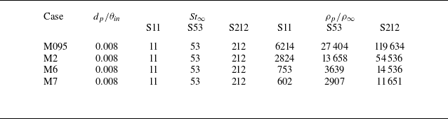The dispersed phase contains three Stokes numbers, $ \textit{St}_\infty =11,53,212$ , with the same particle number $N_p=10^6$ . The particle parameters are set in a similar way to those in Wei et al. (Reference Wei, Wang and Zheng2024). That is, we obtain different particle Stokes numbers $ \textit{St}_\infty$ by varying the particle-to-fluid density ratio from 602 to 119 634. The density ratios used in most cases are higher than those typically encountered in engineering applications, and would be impossible to replicate in experiments. Although $ \textit{St}_\infty$ is also related to particle diameter besides the density ratio and fluid variables, it is difficult to achieve the target Stokes numbers by varying $d_p$ . Large $d_p$ will lead to higher $d_p/\eta$ , where $\eta$ is the Kolmogorov scale, making the point-particle model no longer applicable, while small $d_p$ will lead to higher Knudsen number $K_n=l/d_p$ , causing the continuum assumption of the flow to fail. Therefore, particle diameter 10 $ \mu \textrm{m}$ was chosen, corresponding to a maximum $d_p/\eta \lt 0.25$ across the entire computational domain. The Knudsen number is approximately 0.02, hence the flow falls in the continuum regime (Moss & Bird Reference Moss and Bird1984). Since the volume fraction is $\phi _v\approx 5\times 10^{-7}$ , and the average particle Mach number $ \textit{Ma}_p$ remains below 0.6 for all simulation cases, the employed one-way coupled, shock-free scheme in point-particle simulations is reasonable according to Capecelatro & Wagner (Reference Capecelatro and Wagner2024). For most cases, the mass fraction is less than 1 %. Only in the M095S212 and M2S212 cases is it greater than 2 %. The results from Zhou et al. (Reference Zhou, Zhao, Huang and Xu2020) show that in particle-laden flows, even when the mass fraction reaches 24 %, particles ( $ \textit{St}=30$ ) have a very limited effect on the fluid velocity profile and turbulence intensity. Therefore, we do not consider turbulence modulation in the present study. Detailed parameter settings are provided in table 2.

Table 2.

Particle diameters, Stokes numbers and density ratios.

2.4. Solver verification

To validate the chemical solver with a five-species model, a non-equilibrium decaying isotropic turbulence is simulated, with the details presented in Appendix B. Validation is also conducted based on developing boundary layer simulations. Figure 2(a) shows the profiles of fluid viscosity as compared with Sutherland’s law (Sutherland Reference Sutherland1893). The results in the sub-domain used for verification are obtained within the streamwise range $60\delta_0{-}70\delta _0$ . Close agreement is observed at lower Mach numbers, while the fluid viscosity exhibits a deviation up to 10 % from Sutherland’s predictions in near-wall regions at high Mach number $ \textit{Ma}_\infty =7$ . According to (2.8) and (2.10), this deviation will affect the particle drag and thermophoretic forces. Figure 2(b) shows that the specific heat ratio profiles at $\gamma =1.4$ at free-stream temperature conditions, but decreases significantly at high temperatures, reaching approximately 1.3 in the near-wall region for the case M7.

Figure 2.

The validation of the simulation. (a) Wall-normal distribution of viscosity coefficient compared with Sutherland’s law. (b) Specific heat ratio. (c) The average velocity profiles obtained from the van Driest transformation, compared with the results of Bernardini & Pirozzoli (Reference Bernardini and Pirozzoli2011) at $ \textit{Re}_\tau \approx 450$ , Yu et al. (Reference Yu, Zhao, Yuan and Xu2024) at $ \textit{Re}_\tau = 285{-}504$ , and Wei et al. (Reference Wei, Wang and Zheng2024) at $ \textit{Re}_\theta \approx 670$ . (d) The mean temperature–velocity relationship for the simulated data, compared with the generalised Reynolds analogy (GRA) and the results of Yu et al. (Reference Yu, Zhao, Yuan and Xu2024) in sub-domain $60\delta_0{-}70\delta _0$ .

Due to the compressibility, the traditional wall-unit scaling cannot collapse the velocity profiles. Van Driest (Reference van Driest1951) proposed a well-known transformation to account for the average density effects:

(2.11) \begin{align} u_{\textit{VD}}^+ = \int _0^{\bar {u}^+} \left ( \frac {\bar {\rho }}{\bar {\rho }_w} \right )^{1/2} {\rm d} \bar {u}^+. \end{align}

Figure 2(c) shows the mean turbulent velocity profiles at $ \textit{Ma}_\infty = 0.95$ , 2, 4, 6 and 7 using the van Driest transformation in the sub-domain. The results of Bernardini & Pirozzoli (Reference Bernardini and Pirozzoli2011), Yu et al. (Reference Yu, Zhao, Yuan and Xu2024) and Wei et al. (Reference Wei, Wang and Zheng2024) are also illustrated. For all cases considered, the transformed mean velocity profiles are well collapsed and consistent with the reference data below $y^+=100$ , obeying the linear law in the viscous sub-layer, and the logarithmic law in the log region, as seen in the grey solid line in figure 2(c). The van Driest transformation for the mean velocity also remains valid for high-enthalpy flows by removing the calorically perfect gas assumption, as demonstrated by Duan et al. (Reference Duan, Beekman and Martín2011).

The mean temperature–velocity relationships are shown in figure 2(d), manifesting zero gradients close to the wall due to the quasi-adiabatic thermal condition. The mean temperature profiles are well collapsed at low Mach numbers with Yu et al. (Reference Yu, Zhao, Yuan and Xu2024) and the generalised Reynolds analogy proposed by Zhang et al. (Reference Zhang, Bi, Hussain and She2013), which relates the mean temperature and the mean velocity by

(2.12) \begin{align} \frac {\bar {T}}{T_\infty } = \frac {T_w}{T_\infty } + \frac {T_{r} - T_w}{T_\infty } \frac {\bar {u}}{U_\infty } + \frac {T_\infty - T_{r}}{T_\infty } \left ( \frac {\bar {u}}{U_\infty } \right )^2 \!. \end{align}

The mean temperature–velocity relationship for case M7 exhibits slight downward deviation from the theoretical prediction of the generalised Reynolds analogy. This occurs because the wall temperature under the simulation condition exceeds 2000 K (as shown in table 1), initiating the near-wall dissociation reactions. These endothermic reactions have a chemical cooling effect, thereby reducing the temperature in the flow field. Therefore, it is necessary to take the chemical reactions into account in high-Mach-number flows when calculating the thermophoretic force.

3. The effects of thermophoresis on the transport of particles near the wall

We first present in figure 3 the instantaneous distributions of particle position, streamwise velocity and temperature field within the streamwise range approximately $40\delta_0{-}70\delta _0$ , for case M7S53 as an example. Particles are represented by small grey spheres, and for better visualisation, only parts of particles are shown. Figure 3(a) shows the streamwise turbulent velocity fluctuations normalised by the free-stream velocity $U_\infty$ . The $x$ – $z$ slice at $y^+\approx 15$ clearly highlights the near-wall streak structures. Meanwhile, the $x$ – $y$ slice at $z=0$ reveals that a sharp irregular interface separates the flow field into two distinct red and yellow regions, indicating a jump in velocity (Chauhan, Philip & Marusic Reference Chauhan, Philip and Marusic2014). Figure 3(b) shows the temperature fluctuations normalised by the wall temperature $T_w$ , where travelling-wave-like APNS emerge in the $x$ – $z$ slice at $y^+\approx 3$ . We note that they have also been identified in previous studies through other variables, such as velocity, pressure, dilatation, shear stress and heat flux (Yu et al. Reference Yu, Xu and Pirozzoli2019, Reference Yu, Xu and Pirozzoli2020; Tang et al. Reference Tang, Zhao, Wan and Liu2020; Zhang et al. Reference Zhang, Wan, Dong, Liu, Sun and Lu2023). The spatial scale of APNS is significantly smaller than that of traditional wall streaks. Research indicates that APNS are closely associated with compressibility effects (Yu et al. Reference Yu, Xu and Pirozzoli2019), and they not only significantly influence the statistical characteristics of wall pressure (Zhang et al. Reference Zhang, Wan, Liu, Sun and Lu2022), but are also involved in the mechanisms underlying extreme wall shear stress (Yu et al. Reference Yu, Xu and Pirozzoli2019) and heat flux (Zhang et al. Reference Zhang, Wan, Dong, Liu, Sun and Lu2023).

Figure 3.

Instantaneous snapshot of the flow field and particle distribution within the computational domain $40\delta _0\lt x\lt 70\delta _0$ for case M7S53. Particles are indicated by small grey spheres. (a) Streamwise velocity normalised by the free-stream velocity $U_\infty$ within a vertical slice $z^+=0$ , and the streamwise velocity fluctuations within a horizontal slice at $y^+\approx 15$ . (b) Temperature normalised by the wall temperature $T_w$ at vertical slices $z^+=0$ , and the temperature fluctuations within a horizontal slice at $y^+\approx 3$ .

Figure 4.

The profiles of average particle concentration in the sub-domain ( $60\delta _0\lt x\lt 70\delta _0$ ) for varying $ \textit{St}_\infty$ and $ \textit{Ma}_\infty$ , normalised by the bulk particle concentration: (a) double-logarithmic coordinates, and (b) linear coordinates.

The non-uniform wall-normal distribution of particles can be characterised quantitatively by the mean particle concentration, calculated as

(3.1) \begin{align} c\left (y_{j}\right )=\frac {N_{p}\left (y_{j}\right )}{\sum _{j} N_{p}\left (y_{j}\right )} \frac {\sum _{j} \Delta h_{\kern-1pt j}}{\Delta h_{\kern-1pt j}}, \end{align}

where $N_{p}(y_{j})$ is the particle number located between the $j$ th and $(j+1)$ th vertical grid points, and $\Delta h_{\kern-1pt j}$ is the grid interval. Figure 4(a) shows the time-averaged (in the sub-domain) particle concentration profiles as a function of the inner-scaled wall-normal distance $y^+$ in double-logarithmic coordinates for different Stokes numbers and Mach numbers. Figure 4(b) presents the same particle concentration profiles in linear coordinates. At low Mach numbers ( $ \textit{Ma}_\infty = 0.95$ and 2), the particle concentration exhibits a steep decline with increasing $y^+$ , which can also be observed in figure 4(b), indicating the near-wall accumulation caused by turbophoresis (Sardina et al. Reference Sardina, Schlatter, Brandt, Picano and Casciola2012). This phenomenon becomes most evident at $ \textit{St}_\infty \approx 53$ . The outer-region concentrations are several orders of magnitude lower than those near the wall. The near-wall concentrations for particles with $ \textit{St}_\infty =11$ and $ \textit{St}_\infty =212$ are both lower than those for case $ \textit{St}_\infty =53$ . Such non-monotonic Stokes number effects are consistent with the incompressible results of Bernardini (Reference Bernardini2014). In contrast, the near-wall and outer-region particle concentrations are of comparable magnitude at high Mach numbers. Notably, under the condition $ \textit{St}_\infty =11$ and at high Mach number ( $ \textit{Ma}_\infty = 6$ and 7), the near-wall particle concentration is $c\lt 1$ , resulting in a distinct peak of the particle concentration profile near the wall. Additionally, a small number of particles can be detected beyond the interface due to turbulent dispersion, while most particles accumulate near the wall.

Figure 5.

The instantaneous fields of (a,b) density and (c,d) temperature for cases (a,c) $ \textit{Ma}_\infty = 6$ and (b,d) $ \textit{Ma}_\infty = 7$ . Some typical APNS are marked by boxes.

It is clearly observed that the concentration profiles exhibit distinct peaks at $y^+\approx 3$ within the viscous sub-layer. Sardina et al. (Reference Sardina, Schlatter, Brandt, Picano and Casciola2012) examined the transport of inertial particles for varying particle Stokes numbers in the range $ \textit{St}^+=1{-}100$ in incompressible TBLs. They found that only when $ \textit{St}^+=1$ did the particle concentration exhibit a peak at $y^+\approx 0.4$ . For all other Stokes numbers, the near-wall concentration decreases monotonically with $y^+$ . Bernardini (Reference Bernardini2014) investigated the Reynolds number scaling of particle statistics in turbulent channel flows. No particle concentration peaks were observed at the studied Reynolds numbers $ \textit{Re}_\tau =150{-}1000$ . Yu et al. (Reference Yu, Zhao, Yuan and Xu2024) studied the transport of inertial spherical particles in compressible TBLs and the effects of Mach number, without considering the real gas effects and thermophoretic forces. The peaking phenomenon does not appear even at high Mach number ( $ \textit{Ma}_\infty = 6$ ). The above studies indicate that the effects of Reynolds number, Stokes number and Mach number (only considering compressibility effects, without thermal effects induced by Mach number) are not the reasons for the near-wall concentration peaks. Thus we hypothesise that this phenomenon may be attributed to thermal effects. We further analyse the formation mechanisms of the particle concentration peaks by considering the thermal effects.

Figure 5 shows the instantaneous fields of the density and temperature at the wall ( $y^+\lt 3$ ) for cases $ \textit{Ma}_\infty = 6$ and 7. It is seen that the temperature fluctuation is very low. This is attributed to the isothermal boundary condition imposed on the bottom wall. The zero temperature gradient at the isothermal wall suppresses temperature fluctuations near the wall through thermal conduction. On the contrary, the fluid density fluctuates significantly near the wall. We see that the highest density within the horizontal slice can be up to three times the lowest density. For case $ \textit{Ma}_\infty = 7$ , the APNS are clearly observed, marked by boxes. They are organised as wave-like alternating patterns along the streamwise direction. Nevertheless, a positive correlation between density and temperature is evident.

The APNS in the density and temperature fields directly affect the thermophoretic force near the wall. The magnitude of the thermophoretic force mainly depends on the fluid density because the density appears in the denominator of the thermophoretic force expression. Therefore, the thermophoretic force is more sensitive to changes in fluid density. And the relative temperature difference between the high- and low-temperature regions is very small, i.e. $T_\uparrow \approx T_\downarrow \approx T_0$ , thus the effect of dynamic viscosity can be ignored. According to (2.10), the direction of the thermophoretic force is determined by $\partial T/\partial y$ ; particles in high-temperature ( $T/T_w\gt 1$ ) regions generally experience a downward thermophoretic force, whereas those in low-temperature ( $T/T_w\lt 1$ ) regions are subject to an upward force. We assume that the magnitudes of the temperature gradients in the high- and low-temperature regions are approximately equal but in opposite directions, i.e. $\partial T_\uparrow /\partial y\approx -\partial T_\downarrow /\partial y\approx \partial T/\partial y$ . The average thermophoretic force in the wall-normal direction can be expressed as the average force of particles in the high- and low-density regions:

(3.2) \begin{align} \begin{aligned} \overline {F}_{T,y} = \frac {1}{2}(F_\uparrow + F_\downarrow )&=-\frac {1}{2} \frac {12\pi \mu ^2 r_{\kern-1pt p}C_s \left(\dfrac{\lambda_{\kern-1pt f}}{\lambda _p} + C_t \dfrac{l}{r_{\kern-1pt p}} \right)}{ \left(1 + 3C_m \dfrac{l}{r_{\kern-1pt p}}\right) \left(1 + 2 \dfrac{\lambda_{\kern-1pt f}}{\lambda _p} + 2C_t \dfrac{l}{r_{\kern-1pt p}}\right)}\frac {\partial T}{T_0\,\partial y} \! \left ( \! \frac {1}{\rho _\uparrow } - \frac {1}{\rho _\downarrow } \!\right )\\&= \frac {6\pi \mu ^2 r_{\kern-1pt p}C_s \left(\dfrac{\lambda_{\kern-1pt f}}{\lambda _p} + C_t \dfrac{l}{r_{\kern-1pt p}} \right)}{\left(1 + 3C_m \dfrac{l}{r_{\kern-1pt p}} \right) \left(1 + 2 \dfrac{\lambda_{\kern-1pt f}}{\lambda _p} + 2C_t \dfrac{l}{r_{\kern-1pt p}}\right)}\frac {\partial T}{T_0\,\partial y} \left(\frac {\rho _\uparrow -\rho _\downarrow }{\rho _\uparrow \rho _\downarrow }\right), \end{aligned} \end{align}

where, the subscript $\uparrow$ denotes the high-temperature and high-density regions, and the subscript $\downarrow$ denotes the low-temperature and low-density regions. According to (3.2), the average thermophoretic force is larger than zero, since $\rho _\uparrow \gt \rho _\downarrow$ , meaning that the direction of the average thermophoretic force acting on the particles is away from the wall.

Figure 6.

Joint distribution between normalised density fluctuation $\rho '/\rho _\infty$ and wall-normal particle velocity $v_p/U_\infty$ at the wall ( $y^+\lt 3$ ) for cases (a) M095S53, (b) M2S53, (c) M6S53 and (d) M7S53.

Figure 7.

(a) Schematic of particle transport influenced by the APNS. (b) The ratios of the thermophoretic force to the drag force in the wall-normal direction for different Mach numbers.

Figure 6 further shows the joint distribution of the normalised density fluctuation $\rho '/\rho _\infty =(\rho -\bar {\rho })/\rho _\infty$ and the wall-normal particle velocity $v_p/U_\infty$ at the wall for different Mach numbers, taking $ \textit{St}_\infty =53$ as an example. It can be observed that particles are mainly distributed in the second quadrant ( $\rho '\lt 0$ , $v_p\gt 0$ ) and the fourth quadrant ( $\rho '\gt 0$ , $v_p\lt 0$ ), i.e. in the positive-velocity, low-density region and the negative-velocity, high-density region, confirming the proposed schematic of particle transport influenced by the thermophoretic force as shown in figure 7(a). The schematic illustrates the particle transport mechanism within the distinct temperature and density regions of the APNS: in high-density regions with a positive temperature gradient, particles move towards the wall at a low velocity, whereas in low-density regions with a negative temperature gradient, particles move away from the wall at a high velocity. The wall-normal particle velocity distributions in high- and low-density regions exhibit asymmetry. For example, in low-density regions, the range of wall-normal particle velocity is broader, and extreme values occur more frequently.

Then we performed conditional averaging of the particle velocity in different density regions. For $ \textit{Ma}_\infty = 0.95$ , the results are $|\overline {v_p}(\rho '\lt 0)/U_\infty |=5.48\times 10^{-5}$ and $|\overline {v_p}(\rho '\gt 0)/ U_\infty |=4.27\times 10^{-5}$ . The ratio of the average wall-normal particle velocity in low-density regions to that in high-density regions is 1.28, which is greater than 1, indicating a net upward transport of particles. As the Mach number increases, the ratio increases, reaching 3.03 ( $(6.10\times 10^{-4})/(2.01\times 10^{-4})$ ) at $ \textit{Ma}_\infty = 7$ . Due to the rapid decay of the temperature gradient with height, the magnitude of the thermophoretic force also diminishes quickly, and its range of influence is limited. This accounts for the emergence of the concentration peak near the wall, and its enhancement at higher Mach numbers.

The particle concentration peak at $y^+\approx 3$ for higher Mach numbers in compressible boundary layers is the result of the balance between thermophoresis and turbophoretic drift. The former is related to the thermophoretic force, which depends on temperature and density, while the latter is related to the drag force (Reeks Reference Reeks1983). To illustrate this mechanism, figure 7(b) further shows the ratios of the wall-normal thermophoretic force to the drag force for different Mach number conditions. At low Mach numbers (M095S5, M2S53), the thermophoretic force is significantly smaller than the drag force ( $F_{Ty}/ F_{Dy}\ll 1$ ) and is therefore negligible. Consequently, no near-wall concentration peak is observed. For the high-Mach-number simulations (M6S5, M7S53), the ratio of the thermophoretic force to the drag force first increases and then decreases, reaching its maximum value close to 1 near $y^+\approx 2$ . The concentration peak occurs when the two forces are comparable, which occurs at $y^+\approx 3$ .

4. The effect of Mach number on the transport of particles near the TNTI

Figure 4(b) shows the particle concentration profiles in a linear coordinate to address the outer region. Similar to the findings of Sardina et al. (Reference Sardina, Schlatter, Brandt, Picano and Casciola2012), the concentration profile of finite-inertia particles at low Mach number exhibits a local minimum at $y^+\approx 50$ within the boundary layer. At $y^+\approx 300$ , a maximum value emerges, then particle concentration decays with increasing height, indicating that particles also accumulate near the top of the boundary layer. This accumulation and the minimum $c$ become most pronounced at $ \textit{St}_\infty =53$ for the same Mach number. Additionally, as the Mach number increases, the local minimum values of particle concentration profiles increase, and the particle accumulation near the TNTI weakens. This non-monotonic variation is opposite to the monotonic decrease of particle concentration in channel flow from the wall towards the channel centre (Bernardini Reference Bernardini2014; Wang et al. Reference Wang, Zhou and Zheng2024).

The accumulation of particles occurs at the top of the boundary layer where the TNTI is active (Chauhan et al. Reference Chauhan, Philip and Marusic2014). Therefore, this accumulation is related to the geometric and dynamic properties of the TNTI. We will next focus primarily on the distribution of particles near the TNTI, and how it is influenced by the Mach number. Note that the following discussions are based on the simulation case $ \textit{St}_\infty =53$ because these inertial particles exhibit the most significant accumulation phenomenon. Particles with Stokes numbers $ \textit{St}_\infty =11,212$ also display weak accumulation, but the local accumulations are less pronounced compared to the $ \textit{St}_\infty =53$ case, as shown in figure 4. For this study, accurate identification of the TNTI is essential. The detection of the TNTI relies on characteristic quantities of turbulence, such as the vorticity magnitude (Jahanbakhshi Reference Jahanbakhshi2021), the passive scalar (Kohan & Gaskin Reference Kohan and Gaskin2020) and the turbulence volume (Abreu, Pinho & Silva Reference Abreu, Pinho and da Silva2022). The location of the TNTI depends on the threshold value of the selected criterion. While there are many approaches used in the literature, here we will use the vorticity magnitude ( $\omega ^*=\omega \mu \sqrt {\delta ^+}/\rho u_\tau ^2,\ \omega =\sqrt {\omega _i\omega _i}$ , $\omega _i=\epsilon _{\textit{ijk}}\,\partial u_{\kern-1pt j}/\partial x_k$ , where $\epsilon _{\textit{ijk}}$ is a permutation symbol) as a detector function to identify the TNTI.

Figure 8.

Probability density functions of $\log_{10} \omega ^*$ for cases (a) $ \textit{Ma}_\infty =0.95$ , (b) $ \textit{Ma}_\infty =2$ , (c) $ \textit{Ma}_\infty =6$ and (d) $ \textit{Ma}_\infty =7$ .

Figure 8 shows the probability density functions of the dimensionless vorticity magnitude $\log_{10}\omega^*$ within the sub-domain for all four Mach number cases, as a function of the wall-normal distance $y/\delta$ . Taking the low-Mach-number case M095S53 as an example, two regions with high-probability-density distributions of $\log_{10}\omega^*$ can be observed. The region in the lower right corner is the near-wall high-vorticity region, and that in the upper left corner is actually the free flow with very low vorticity value due to the finite accuracy of the numerical scheme. The interlock of two iso-probability-density contours is selected as the threshold for TNTI identification. The vorticity value corresponding to the white dashed line in figure 8 represents the threshold used to detect the TNTI. The vertical coordinate corresponding to the intersection point is the average interface height $\bar {y}_{\textit{TNTI}}$ . We can see that the threshold vorticity gradually decreases as the Mach number increases because the $x$ -coordinate corresponding to the white dashed line shifts to the right. Specifically, the thresholds $\log_{10}\omega^*_{th}$ for $\log_{10}\omega^*$ are approximately $-1.4,-1.3,-1.2,-1.1$ for the cases M095S53, M2S53, M6S53, M7S53 in figures 8(a–d), respectively. The threshold vorticity values are used across the entire analysis sub-domain to identify the TNTI, as the vorticity iso-surfaces.

Figure 9.

Three-dimensional iso-surfaces of vorticity, taking $ \textit{Ma}=7$ as an example. The structures identified as ’bubbles’ and ’droplets’ are coloured in blue, while the TNTI is coloured in black.

In figure 9, we visualise the three-dimensional instantaneous vorticity iso-surface identified by the threshold vorticity $\omega _{th}^*$ for particle-free case M7. The largest connected iso-surface, coloured in black, is identified as the TNTI in this work; it envelops the turbulent core region. Numerous isolated ‘bubbles’ can be seen within the flow field beneath the TNTI, along with several ‘droplets’ in the potential flow region above it. Both bubbles and droplets are three-dimensional structures with roughly comparable size in all directions. In fact, bubbles are localised low-vorticity regions (swallowed irrotational flow) associated with engulfment of the TNTI, which refers to the process where the irrotational flows are swallowed into the TBL (Jahanbakhshi Reference Jahanbakhshi2021), while droplets are localised high-vorticity regions in the potential flow.

Figure 10.

Threshold iso-surfaces identified by the vorticity method, with droplets and bubbles, for cases (a) M095S53, (b) M2S53, (c) M6S53 and (d) M7S53.

However, adding particles to the three-dimensional visualisation in figure 9 for particle-laden flow would reduce clarity, making it unsuitable for analysing the entire TNTI as well as the bubbles and droplets near the TNTI. Therefore, we ultimately adopted two-dimensional diagrams to present the results. Figure 10 shows the instantaneous vorticity $\omega ^*$ distribution in the $x{-}y$ plane for all the cases at $z^+=0$ . The largest single connected component of the vorticity iso-surface that divides the turbulent and non-turbulent regions (Borrell & Jimenez Reference Borrell and Jimenez2016) is identified as the TNTI (black solid line in figure 10). We see that the TNTI is wrinkled and exhibits spatial undulation with the engulfment of large-scale structures (Silva et al. Reference da Silva, Hunt, Eames and Westerweel2014).

As the Mach number increases, the large-scale undulation of the TNTI becomes more significant. We calculated the standard deviation $\sigma _{\textit{TNTI}}$ of the TNTI height $y_{\textit{TNTI}}$ . The results show that values are $\sigma _{\textit{TNTI}}/\bar {y}_{\textit{TNTI}} = 0.19$ , 0.20, 0.24 and 0.27 for $ \textit{Ma}_\infty = 0.95$ , 2, 6 and 7, respectively. The large-scale undulation is related to the large-scale structures in the outer region of wall-bounded turbulence. As the Mach number increases, the scale of these large-scale structures increases (Wang et al. Reference Wang, Zhou and Zheng2024), which also leads to more pronounced undulation. In addition, the wrinkled TNTI has fractal characteristics. The box-counting algorithm (Sreenivasan & Meneveau Reference Sreenivasan and Meneveau1986; Sreenivasan & Prasad Reference Sreenivasan and Prasad1989; Sreenivasan, Ramshankar & Meneveau Reference Sreenivasan, Ramshankar and Meneveau1989; Meneveau & Sreenivasan Reference Meneveau and Sreenivasan1990) is used to calculate the fractal dimension $D_{\kern-1pt f}$ ; see Appendix C for details. The results are $D_{\kern-1pt f}=2.21$ , 2.18, 2.15 and 2.13 for $ \textit{Ma}_\infty =0.95$ , 2, 6 and 7. Note that Su et al. (Reference Su, Long, Wang and Li2024) reported $D_{\kern-1pt f}=2.18$ in compressible flow at $ \textit{Ma}_\infty = 2.9$ . The decreased $D_{\kern-1pt f}$ indicates that as the Mach number increases, the TNTI becomes less wrinkled, which is revealed for the first time. Additionally, it can be observed that the number of droplets and bubbles also increases with Mach number, which may be due to enhanced compressibility at higher Mach numbers (Duan et al. Reference Duan, Beekman and Martín2011). This enhanced compressibility leads to velocity discontinuities and local extrema in vorticity. Because droplets and bubbles are local high- and low-vorticity regions, respectively, the increase in the probability of local extrema in vorticity leads to an increase in the number of identified high- and low-vorticity regions, i.e. bubbles and droplets.

Figure 11.

Snapshots of the TNTI in the $x$ – $y$ plane at $z^+=0$ , with the TNTI marked in black. Particles are indicated by dots and coloured by their wall-normal velocity in a quasi-two-dimensional slice across the $z^+=0$ plane, for cases (a) M095S53, (b) M2S53, (c) M6S53 and (d) M7S53.

Obviously, the two features – the wrinkled TNTI with large-scale undulations, and the bubbles/droplets – are related to the transport of particles. We first look at the effect of the TNTI itself on the particle transport. Figure 11 shows the identified TNTI and particle distribution near the TNTI for cases M095S53, M2S53, M6S53 and M7S53. The TNTI is marked in black, and particles are coloured by their wall-normal velocity $v_p/U_\infty$ . Red particles ( $v_p\gt 0$ in figure 11) indicate that particles move upwards, while blue particles indicate downward transport. Several features can be observed. First, particle distribution in the turbulent region exhibits non-uniform structures with void regions below the TNTI, which is influenced by the large-scale structures in the outer turbulent region. Second, a significant high particle concentration is observed near the TNTI, implying particle accumulation. This phenomenon is consistent with the simulation results of incompressible-particle-laden TBLs (Wei et al. Reference Wei, Wang and Zheng2024). Through the vorticity analysis, Wei et al. (Reference Wei, Wang and Zheng2024) suggested that the particles tend to accumulate below the interface due to the centrifugal effect of large-scale vortices in the outer region of wall turbulence and the combined barrier effect of potential flow. Figure 11 shows that the results are qualitatively consistent across different Mach numbers. Third, for all cases, the red particles with upward velocity are mainly distributed on the bulges of the TNTI, while the blue particles with downward velocity are primarily distributed near the inward cusps. This means that the smooth bulges and the inward cusps transport particles upwards and downwards, respectively.

Figure 12.

(a) Particle flux near the TNTI variation with the interface height. (b) The conditionally averaged particle concentration profiles. The inset in (b) shows the averaged particle wall-normal velocity.

To quantify this transport effect, we show in figure 12(a) the particle flux $c_{\textit{TNTI}}v_p$ on the TNTI, scaled by the free-stream velocity $U_\infty$ , where $c_{\textit{TNTI}}$ is the particle concentration at the position of the TNTI. The horizontal coordinate in the figure is normalised by the mean interface height $\bar {y}_{\textit{TNTI}}$ for each case. We can see that $c_{\textit{TNTI}}v_p/U_\infty \lt 0$ at low $y_{\textit{TNTI}}/\bar {y}_{\textit{TNTI}}$ , while $c_{\textit{TNTI}}v_p/U_\infty \gt 0$ at high $y_{\textit{TNTI}}/\bar {y}_{\textit{TNTI}}$ . By summing $c_{\textit{TNTI}}v_p$ , we find that overall, particles are transported upwards on the interface, since the mean particle flux $\overline {c_{\textit{TNTI}}v}_p/U_\infty$ is slightly ${\gt } 0$ for all the cases. This is likely because the average interface height increases along the streamwise direction, which is similar to the boundary layer thickness. Note that although the mean particle fluxes in TBLs at different Mach numbers are almost the same when $y_{\textit{TNTI}}/\bar {y}_{\textit{TNTI}}\gt 1$ , their magnitude decreases with increasing Mach number when $y_{\textit{TNTI}}/\bar {y}_{\textit{TNTI}}\lt 1$ . This indicates a weakened downward particle transport at high Mach numbers.

Figure 12(b) shows the conditionally averaged particle concentration $c_{cond}$ near the TNTI as a function of normalised distance away from the TNTI $\xi /\delta$ , with $\xi /\delta \gt 0$ indicating the non-turbulent region, and $\xi /\delta \lt 0$ indicating the turbulent region. The normal distance is defined as $\xi =(x_p-x_{IB})n_{IB}$ , where $x_p$ is the particle position coordinate, $x_{IB}$ is the position of the nearest TNTI point to the particle, and $n_{IB}$ is the normal direction at this TNTI point. The local normal vector to the interface is computed as $n = -\boldsymbol{\nabla }\omega ^2 / \|\boldsymbol{\nabla }\omega ^2\|$ , and $c_{cond}$ is normalised by the averaged particle concentration on the TNTI $\bar {c}_{\textit{TNTI}}$ . We see that there is a peak ( $c_{cond}/\bar {c}_{\textit{TNTI}}\gt 1$ ) of particle concentration for each case at $\xi /\delta \lt 0$ , indicating that particles accumulate on the turbulent side of the interface. For $ \textit{Ma}_\infty =0.95, 2, 6, 7$ , the peak values of $c_{cond}/\bar {c}_{\textit{TNTI}}$ are $1.11$ , $1.06$ , $1.02$ , $1.01$ , respectively, and they are located at $\xi /\delta \approx -0.031$ , $-0.025$ , $-0.012$ , $-0.008$ . This means that the peak in particle concentration beneath the interface diminishes, and the concentration peak shifts closer to the TNTI as the Mach number increases, which is consistent with the accumulation phenomenon of the ensemble-averaged concentration shown in figure 4. This is because at high Mach numbers, the vorticity fluctuations in wall-bounded turbulence decrease (Yu et al. Reference Yu, Xu and Pirozzoli2019), the centrifugal effect weakens, and consequently, the ability to transport particles upward is suppressed. This can also be seen from the distribution of the particle wall-normal velocity $v_p/U_\infty$ for different Mach numbers shown in figure 12(b). It is seen that the particle velocity is $v_p/U_\infty \gt 0$ below the TNTI. However, as the Mach number increases, its magnitude decreases. Note that since the TNTI is far away from the wall, the influence of temperature on particle transport is less pronounced.

Figure 13.

Schematic of engulfment and particle transport for case M7S53.

Now we move to the relationship between the bubbles/droplets and the transport of particles. Due to the limited number of droplets, we discuss only the bubbles on the turbulent side. Figure 13 shows the vorticity and particle distribution for case M7S53 around bubbles in a typical engulfment region. In this figure, the black arrows indicate the vectors $(u_p-u_f,v_p)$ of the particle wall-normal velocities $v_p$ and the streamwise slip velocities $u_p-u_f$ , where $u_f$ is the fluid velocity at the particle position obtained by trilinear interpolation. It is seen that the particles near the bubbles tend to move downwards. Meanwhile, the particles are mainly distributed below these bubbles, and exhibit large velocity magnitudes, as indicated by the longer arrows.

For the quantitative analysis of particle distribution around bubbles, we use the clustering method (Chen et al. Reference Chen, Dong, Chen, Yuan and Xu2021) to identify bubbles, i.e. we first binarise the vorticity field of the flow into the labels $I=0$ and $I=1$ , corresponding to $\omega ^*\gt \omega _{th}^*$ and $\omega ^*\lt \omega _{th}^*$ , respectively. Because the vorticity in the bubble region is less than $\omega _{th}^*$ , the boundary of a bubble encloses a region $I=1$ . Then each identified connected region is considered as one bubble. Subsequently, we perform a conditional average of the surrounding particles using the bubbles as events. The specific process for conditional averaging is as follows. For an event $E(\chi ^*)$ defined at a bubble position $\chi ^*$ , which is the centre of the bubble, the conditional average of a quantity $\psi$ at a location $\chi$ is given by $\langle \psi (\chi )\,|\,E(\chi ^*)\rangle =\sum \psi _i(\chi )/E_n$ , where $E_n$ is the number of events. We are currently interested in the local particle volume fraction around the bubbles, thus $\psi$ denotes the local particle volume fraction $\phi _{\textit{bub}}$ and the label $I$ .

Figure 14.

Contour plots of particle volume fraction around bubbles for cases (a) M095S53, (b) M2S53, (c) M6S53 and (d) M7S53.

Figure 14 shows the conditional average volume fraction $\phi _{\textit{bub}}/\phi _v$ and the bubble for cases M095S5, M2S53, M6S53 and M7S53. The centre of the mean bubble is marked with a black star. The shape of the mean bubble is shown as a black solid line. We note that the solid line is the iso-line of $\langle I\rangle =0.01$ because we just obtain the contours of binarised $I$ ; when performing event averaging, the obtained $\langle I\rangle$ may not be an integer. The conditional particle volume fraction $\phi _{\textit{bub}}/\phi _v$ is represented with a flood contour. We see from figure 14(a) that the mean bubble is ellipse-like and tilted, with inclination angle $40^\circ$ from the abscissa. High $\phi _{\textit{bub}}/\phi _v$ appears at the lower downstream region of the bubble, indicating particle accumulation there. We try to explain the phenomena according to the engulfment process and particle inertia. As a matter of fact, the bubbles and the downward transport of particles are both the result of the engulfment process of the TNTI. However, the moving inertia forces particles to continuously move downwards after going into the turbulent region from the trough of the TNTI, and ultimately they move to a lower position than the irrotational fluid in bubbles. Analogously, these particles move with high streamwise velocity because they come from the high-speed potential flow region and move faster than the fluid, and therefore faster than the bubbles with zero inertia, in the turbulent region. That is why the high conditional $\phi _{\textit{bub}}/\phi _v$ is observed downstream of the bubbles. We also noticed that particles are seldom detected within the bubble, as shown in figure 13, and $\phi _{\textit{bub}}/\phi _v\sim 1$ within the mean bubble, indicating that the low vorticity bubbles may repel particles since the height with dense bubbles is just where the beneath-TNTI particle accumulation appears.

As the Mach number increases, the mean bubble becomes circular-like and its inclination angle increases. In fact, the inclination angle is $46^\circ , 59^\circ , 69^\circ$ for cases M2S53, M6S53 and M7S53. This is attributed to the reduced fractal dimension. The complexity of the interface is reduced, and the bubbles become smooth. Meanwhile, the inclination angle of the $\phi _{\textit{bub}}/\phi _v$ contour increases, while the maximum $\phi _{\textit{bub}}/\phi _v$ decreases from 1.46 to 1.25 as the Mach number increases from 0.95 to 7.0. The latter can be explained by figure 12(a): on the TNTI, the value of the particle flux near the inward cusps decreases with increased Mach numbers, which reduces the number of particles swallowed into the turbulent region.

5. Non-uniform distribution of particles in the horizontal plane

Most of the horizontal distribution phenomena observed in incompressible particle-laden wall-bounded turbulence are also present in compressible TBLs with thermal effects. In the near-wall region, particles form streaks in the horizontal plane, and preferentially distribute in low-speed regions. Meanwhile, particles form organised structures and distribute in high-speed regions in the outer layer.

Figure 15.

Instantaneous streamwise velocity fluctuation $u'/U_\infty$ with particles near the wall ( $y^+\approx 3$ ), for cases (a) M095S53 and (b) M7S53. (c) Two-point correlation of particle number density in the spanwise direction at reference height $y^+\approx 3$ .

In figures 15(a) and 15(b), we present the distributions of the dimensionless streamwise fluctuation velocity $u'/U_\infty$ near the wall at $y^+\approx 3$ for cases M095S53 and M7S53. Particles are coloured by their wall-normal velocity $v_p/U_\infty$ . For a better presentation of spatial distribution, particles are enlarged. Clear particle streak structures are observed in the low Mach number case. However, at high Mach number, these streak structures become less pronounced. To emphasise this phenomenon, we calculated the two-point correlation coefficient $R_{\varPhi ^{\prime } \varPhi ^{\prime }}$ of the particle number density $\varPhi$ to quantify the particle structures. The coefficients are defined as $ R_{\varPhi ^{\prime } \varPhi ^{\prime }}(\Delta z)=\left \langle \varPhi ^{\prime } (x, y_{\mathit{ref}}, z, t )\, \varPhi ^{\prime } (x, y_{\mathrm{ref}}, z+\Delta z, t )\right \rangle /\left \langle \varPhi ^{\prime } (x, y_{\mathit{ref}}, z, t )\, \varPhi ^{\prime } (x, y_{\mathit{ref}}, z, t )\right \rangle ,$ where $y_{\mathit{ref}}$ is the reference height. Figure 15(c) shows that the position of the first local minimum value in the spanwise two-point correlations for $ \textit{Ma}_\infty =0.95$ occurs at $\Delta z^+\approx 61$ , implying an average spanwise spacing of approximately 122 viscous units, along with the results of Sardina et al. (Reference Sardina, Schlatter, Brandt, Picano and Casciola2012). As the Mach number increases, this spacing increases, reaching approximately 130, 141 and 147 viscous units for $ \textit{Ma}_\infty =2$ , 6 and 7, respectively. Moreover, the minimum value of the spanwise two-point correlation increases from −0.095 to −0.042, suggesting an attenuation of the particle streaks with increasing Mach number. This may be due to the weakened quasi-streamwise vortices and consequently reduced capacity to organise particles into streaks (Wang et al. Reference Wang, Zhou and Zheng2024; Yu et al. Reference Yu, Zhao, Yuan and Xu2024).

Figure 16.

(a,b) Instantaneous streamwise velocity fluctuation $u'/U_\infty$ at $y^+\approx 200$ with particles near the TNTI ( $175 \lt y^+\lt 225$ ), and (c,d) the iso-surfaces obtained by applying the selected vorticity magnitude threshold with the same particles, for cases (a,c) M095S53 and (b,d) M7S53.

Furthermore, an enlarged view of figure 15(b) shows the particle distribution near the APNS compared with that without APNS in figure 15(a). The particles are coloured by their wall-normal velocity, with white and black dots representing high- and low-velocity magnitudes, respectively. It can be observed that particles near the APNS exhibit higher-velocity magnitudes. This is attributed to the flow disturbance induced by the APNS at high Mach numbers, as shown in figure 7. These high-velocity-magnitude particles tend to move upwards and downwards, drifting away from the particle streaks and thereby depleting the streaks.

Figures 16(a) and 16(b) show the instantaneous streamwise velocity fluctuation $u'/U_\infty$ at $y^+\approx 200$ with the particle distribution near the TNTI ( $175\lt y^+\lt 225$ ). Particles tend to distribute in high-speed regions, consistent with the results of Xiao et al. (Reference Xiao, Jin, Luo, Dai and Fan2020) for compressible TBLs. At low Mach numbers, particles maintain organised structures in the outer region, consistent with the findings of Wang & Richter (Reference Wang and Richter2019) for incompressible open-channel turbulence. As the Mach number increases, the organised structures become less clear. This may be attributed to enhanced flow fluctuations caused by pronounced genuine compressibility effects at high Mach numbers (Yu et al. Reference Yu, Xu and Pirozzoli2019). Figures 16(c) and 16(d) show the top views of the vorticity iso-surfaces, which are obtained using the selected vorticity magnitude threshold $\omega ^*_{th}$ and coloured by the instantaneous values of the interface height $y_{\textit{TNTI}}$ . The particles are the same as those in figures 16(a) and 16(b). A comparison between figures 16(c) and 16(a) reveals an inverse correlation between flow velocity and TNTI height: low-speed regions correlate with high-interface-height regions, and vice versa. This phenomenon can be attributed to the occurrence of sweep and ejection events, which induce a correlation between high-speed regions and low-interface-height regions. Particles in the outer region tend to distribute in high-speed regions. These high-speed regions correspond to low-interface-height regions, known as inward cusps. Consequently, the particles preferentially distribute in these inward cusps. Furthermore, small-scale wrinkles located on large-scale bulges and inward cusps were observed at $ \textit{Ma}_\infty = 0.95$ . This is similar to the observation in Wei et al. (Reference Wei, Wang and Zheng2024) for incompressible TBLs. However, these wrinkles became less pronounced at $ \textit{Ma}_\infty = 7$ . Comparison of figures 16(c) and 16(d) shows that particles are distributed over a larger area in the inward cusps as the Mach number increases, which is likely caused by the reduction of wrinkles.