1. Introduction
Shock wave/boundary layer interaction (SBLI) is a classic flow phenomenon for a high-speed vehicle. The boundary layer in the internal and external flows of a vehicle may frequently encounter shock waves, leading to boundary layer separation, extreme heating loads, unsteadiness, transition to turbulence, and so on. There are numerous configurations where SBLI occurs, such as impinging shock, compression ramp, swept ramp, double cone and single fin (Gaitonde Reference Gaitonde2015). Understanding the dynamics of SBLI over different configurations is of crucial importance to the design and flow control of supersonic and hypersonic vehicles. According to the state of the incoming boundary layer, SBLI can be classified into three groups (Gaitonde & Adler Reference Gaitonde and Adler2023): shock wave/laminar boundary layer interaction (SLBLI), shock wave/transitional boundary layer interaction (STrBLI) and shock wave/turbulent boundary layer interaction (STBLI). Although STBLI has been comprehensively studied for decades (Dolling Reference Dolling2001; Clemens & Narayanaswamy Reference Clemens and Narayanaswamy2014; Gaitonde & Adler Reference Gaitonde and Adler2023), the other two interactions have been less investigated until recent years, especially in the framework of laminar–turbulent transition.
1.1. The SLBLI
In general, SLBLI is found in a low-disturbance environment (e.g. quiet wind tunnel, some flight conditions) and can be extensively simulated by computational fluid dynamics (CFD). In SLBLI, the laminar boundary layer is hard to resist the shock-induced adverse pressure gradient, and as a result, a considerable separation bubble is usually produced. Due to the presence of a separation bubble, the reattached boundary layer may transition to turbulence because of different instabilities.
First, the separation bubble (i.e. the recirculating flow in the bubble) may be associated with self-excited instability that induces streamwise streaks downstream of reattachment in the absence of external disturbances (Hildebrand et al. Reference Hildebrand, Dwivedi, Nichols, Jovanović and Candler2018; Sidharth et al. Reference Sidharth, Dwivedi, Candler and Nichols2018; Cao et al. Reference Cao, Hao, Klioutchnikov, Olivier and Wen2021). These streaks can finally break down to turbulence due to secondary instability (Fu et al. Reference Fu, Karp, Bose, Moin and Urzay2021; Cao et al. Reference Cao, Hao, Klioutchnikov, Wen, Olivier and Heufer2022). As the linear behaviour of self-excited instability can be predicted by global stability analysis (GSA) (Theofilis Reference Theofilis2011), it is also called global instability (Hao et al. Reference Hao, Cao, Wen and Olivier2021). The occurrence of global instability in different SBLIs – e.g. impinging shock case (Robinet Reference Robinet2007), double-wedge flow (Sidharth et al. Reference Sidharth, Dwivedi, Candler and Nichols2018), double-cone flow (Hao et al. Reference Hao, Fan, Cao and Wen2022), backward-facing step flow (Yu et al. Reference Yu, Hao, Wen and Xu2024), hollow-cylinder–flare flow (Li & Hao Reference Li and Hao2023) and compression-ramp flow (Cao et al. Reference Cao, Hao, Klioutchnikov, Olivier and Wen2021) – has been reported. For a flow over a compression ramp (or compression corner), the occurrence of global instability may be observed by increasing the ramp angle (Hao et al. Reference Hao, Cao, Wen and Olivier2021).
If the separation bubble is intrinsically stable, then convective instabilities can also be at play and trigger transition to turbulence in an SLBLI. In terms of a high-speed boundary layer, there exist multiple paths to turbulence, such as eigenmode growth, transient growth and bypass mechanisms (Reshotko Reference Reshotko2008). Essentially, these transition paths are also applicable to SLBLI. For example, a pair of Mack’s first modes can nonlinearly lead to the formation of streamwise streaks, which then break down to turbulence over the compression ramp (Lugrin et al. Reference Lugrin, Beneddine, Leclercq, Garnier and Bur2021; Dwivedi, Sidharth & Jovanović Reference Dwivedi, Sidharth and Jovanović2022). In addition to Mack’s first mode, Mack’s second mode can also play a role at high Mach numbers (Butler & Laurence Reference Butler and Laurence2021; Paredes et al. Reference Paredes, Scholten, Choudhari, Li, Benitez and Jewell2022). Besides, both the first mode and second mode are found to contribute to the transition process in a cone–cylinder–flare geometry (Benitez et al. Reference Benitez, Borg, Paredes, Schneider and Jewell2023a ,Reference Benitez, Borg, Scholten, Paredes, McDaniel and Jewell b ; Caillaud et al. Reference Caillaud2024). Furthermore, streamwise streaks may arise via transient growth then experience strong amplification in the interaction region due to Görtler instability (Cao et al. Reference Cao, Hao, Guo, Wen and Klioutchnikov2023; Hao et al. Reference Hao, Cao, Guo and Wen2023). Therefore, the transition process associated with the convective instabilities is highly case-dependent. In addition, the transition path is also dependent on the amplitude of external disturbances (Cao, Hao & Guo Reference Cao, Hao and Guo2024). It should be mentioned that in an experiment, global instability and convective instability may coexist and influence each other (Cao et al. Reference Cao, Hao, Guo, Wen and Klioutchnikov2023). Their combined effect is receiving more attention.
1.2. The STrBLI
Unlike SLBLI, for which the transition to turbulence usually appears downstream of the SBLI region, the transition in STrBLI is associated with the SBLI. As a consequence, the boundary layer in the SBLI region is highly transitional, thus can withstand a higher adverse pressure gradient. Therefore, the separation bubble observed in STrBLI is usually smaller than its counterpart in SLBLI, and the surface heating loads near reattachment also exhibit a significant difference between STrBLI and SLBLI. A comprehensive review on STrBLI can be found in Knight & Mortazavi (Reference Knight and Mortazavi2018).
Concerning the effects of external disturbances on boundary layer separation, data are rarely available for a direct comparison of the separation bubble size between SLBLI and STrBLI because only a few wind tunnels can operate at both noisy and quiet conditions. A recent work by Benitez, Jewell & Schneider (Reference Benitez, Jewell and Schneider2021) provided an example. However, it is easy to change the Reynolds number in an experiment so as to study its influence on the boundary layer separation. Although the separation bubble grows with increasing Reynolds number in SLBLI, the trend that the separation bubble size decreases with increasing Reynolds number for STrBLI has been reported in numerous experimental studies (e.g. Sandham et al. Reference Sandham, Schülein, Wagner, Willems and Steelant2014; Schülein Reference Schülein2014; Willems, Gülhan & Steelant Reference Willems, Gülhan and Steelant2015; Lugrin et al. Reference Lugrin, Nicolas, Severac, Tobeli, Beneddine, Garnier, Esquieu and Bur2022; Benitez et al. Reference Benitez, Caillaud, McDaniel, Lugrin, Borg, Jewell, Scholten, Paredes, Li and Choudhari2024). Therefore, the difference in the size of the separation bubble serves as a typical feature to distinguish between SLBLI and STrBLI.
Another feature of STrBLI is the greater surface heat transfer than in laminar and turbulent interactions, which has been demonstrated in the literature (Benay et al. Reference Benay, Chanetz, Mangin, Vandomme and Perraud2006; Bur & Chanetz Reference Bur and Chanetz2009; Knight & Mortazavi Reference Knight and Mortazavi2018; Currao et al. Reference Currao, Choudhury, Gai, Neely and Buttsworth2020). This heat-flux overshoot can be as high as 15 % (Currao et al. Reference Currao, Choudhury, Gai, Neely and Buttsworth2020) to 25 % (Lugrin et al. Reference Lugrin, Nicolas, Severac, Tobeli, Beneddine, Garnier, Esquieu and Bur2022). An impact of the overshoot is significant thermal loads on the vehicle. It is therefore suggested by Benay et al. (Reference Benay, Chanetz, Mangin, Vandomme and Perraud2006) and Bur & Chanetz (Reference Bur and Chanetz2009) that provoking transition to obtain a fully STBLI could be preferable. The causes of heat-flux overshoot are often related to the Görtler instability pertaining to the streamline curvature at reattachment (Benay et al. Reference Benay, Chanetz, Mangin, Vandomme and Perraud2006; Currao et al. Reference Currao, Choudhury, Gai, Neely and Buttsworth2020) as well as the rapid transition at reattachment. Other instabilities involving the transition process in STrBLI include the first mode (Yao et al. Reference Yao, Krishnan, Sandham and Roberts2007; Lugrin et al. Reference Lugrin, Beneddine, Leclercq, Garnier and Bur2021), the second mode (Sandham et al. Reference Sandham, Schülein, Wagner, Willems and Steelant2014) and the global instability (Lugrin et al. Reference Lugrin, Nicolas, Severac, Tobeli, Beneddine, Garnier, Esquieu and Bur2022). In general, the underlying transition mechanisms are also case-dependent and rely on both flow conditions and configurations. Therefore, much effort is required towards a deep understanding of the transition mechanisms in both SLBLI and STrBLI.
1.3. Difficulties in studying SLBLI and STrBLI
One difficulty in studying the transition to turbulence in SBLI is the determination of freestream disturbances. As the noise level in different facilities differs, achieving cross-validation of experimental data is challenging. Moreover, a lack of full information on wind-tunnel disturbances and free-flight disturbances makes it difficult to simulate SBLI using CFD. On the other hand, the transition path is sensitive to the nature of external disturbances. Therefore, it is necessary to identify the details (e.g. amplitude, frequency, wavenumber) of disturbances for different flows. Although random forcing may represent the noise in some situations (e.g. some flight conditions), the disturbances in conventional wind tunnels have particular characteristics (Laufer Reference Laufer1961; Duan et al. Reference Duan2019). With the development of measurement techniques, it is now possible to obtain more information about the disturbances in wind tunnels (Duan et al. Reference Duan2019).
Although great progress has been achieved in SLBLI and STrBLI in recent years, there are no evident criteria to distinguish between SLBLI and STrBLI. It is usually believed that for an STrBLI, the transition happens at reattachment (Knight & Mortazavi Reference Knight and Mortazavi2018), and for an SLBLI, it takes place downstream of reattachment (Cao et al. Reference Cao, Hao, Klioutchnikov, Wen, Olivier and Heufer2022, Reference Cao, Hao and Guo2024). However, this statement seems ambiguous as there is no exact description about the transition zone, i.e. the transition onset and end. If the transition zone is clearly identified, then it might be possible to provide more physical insights on the boundary layer separation, heat-flux overshoot, transition mechanism, and so on.
In the present work, we study a canonical SBLI – compression-ramp flow – at Mach 6.5. Wind tunnel experiments, numerical simulations and stability analyses will be carried out to reveal the complete transition process for different disturbance levels. Two distinct transition scenarios will be demonstrated. One is related to SLBLI, and the other is associated with STrBLI. Although the two scenarios are often observed in experimental and numerical studies, the direct comparison between SLBLI and STrBLI is still rare. More importantly, we will uncover the relative position between the reattachment region and the transition zone. On the basis of our findings, a criterion is proposed to distinguish between SLBLI and STrBLI.
2. Experimental and numerical methodology
2.1. Experimental set-up
The experiments presented in this study were conducted in the JF8A shock tunnel, a medium-scale hypersonic facility located at the Institute of Mechanics, Chinese Academy of Sciences. The JF8A is a pulsed hypersonic tunnel designed for dual-mode operation, capable of functioning as both a shock tunnel and a gun tunnel. The facility comprises a high-pressure driver section, a low-pressure driven section, a hypersonic nozzle, a test section and a downstream vacuum tank. The inner diameters of the driver and driven sections are 150 and 155 mm, respectively, with corresponding lengths 9.67 and 16.6 m. The JF8A has been widely employed in studies involving hypersonic heat transfer, SBLI and boundary layer transition (Wang et al. Reference Wang, Lu, Li, Wu, Li, Zhao and Jiang2017).
The specific test conditions for the present experiments are summarised in table 1, corresponding to freestream Reynolds number
 $1.2\times 10^7$
 $\text{m}^{-1}$
and Mach number 6.5. The test model is a typical
 $15^\circ$
compression ramp, with width 300 mm and total length 346 mm. The length of the flat plate is
 $L^* = 100$
mm, which is used as the reference length in this paper. As a result, the corner is located at
 $x = x^*/L^* = 1$
. It is noted that the dimensional variables in the present paper are highlighted with an asterisk superscript. Other variables are non-dimensional. Thin-film resistance gauges were mounted on the model because of their fast thermal response and high electrical sensitivity to temperature variations. The measured voltage signals were converted to time-resolved surface heat flux using a thermoelectric analogue network. In addition, the freestream density disturbances were measured using the focused laser differential interferometry (FLDI) technique. Detailed descriptions of the FLDI measurement set-up can be found in Huang et al. (Reference Huang, Zhang, Liu, Luo, Wang, Wang and Zhao2025b
).
Flow conditions at the shock tunnel JF8A.

2.2. Direct numerical simulations
Direct numerical simulations (DNS) are also employed to investigate the transition scenarios in the compression-ramp flow. The Navier–Stokes equations for unsteady, compressible flow are discretised by a finite-difference method with high-order accuracy. A fifth-order weighted essentially non-oscillatory (WENO) scheme and a sixth-order central-difference scheme are utilised for inviscid and viscous fluxes, respectively. The time integration is approximated by a third-oder Runge–Kutta scheme. Details about the numerical scheme and the validation of the DNS solver may be found in Cao et al. (Reference Cao, Klioutchnikov and Olivier2019, Reference Cao, Klioutchnikov and Olivier2020, Reference Cao, Hao, Klioutchnikov, Olivier and Wen2021, Reference Cao, Hao, Klioutchnikov, Wen, Olivier and Heufer2022) and Cao (Reference Cao, Hao, Klioutchnikov, Olivier and Wen2021).
In the simulation, a total number of
 $3200 \times 320 \times 260 \approx 266 \text{ million}$
grid points is used to capture the transition process. Freestream parameters are introduced at the inflow and upper boundaries. A zero-gradient boundary condition is used at the outflow boundary. For the no-slip wall, an isothermal condition with wall temperature 293 K is specified. A periodic boundary condition is used in the spanwise direction (
 $z$
). The time step is set at
 $4.7 \times 10^{-9}$
s to satisfy the Courant–Friedrichs–Lewy condition. To save computational resources, the width of the compression ramp is set at 14 mm. This choice is based on the stability analysis result that will be shown later. While keeping the same flat-plate length, the length of the ramp in the DNS is different to that in the experiments.
2.3. The GSA
To examine the global instability of the considered compression-ramp flow, GSA is employed to study the temporal stability of the two-dimensional (2-D) base flow with respect to three-dimensional (3-D) small-amplitude perturbations. First, the Navier–Stokes equations are linearised and written in the operator form
 \begin{align} \frac {\partial \boldsymbol{U}'}{\partial t} = \boldsymbol{A} \boldsymbol{U}', \end{align}
where
 $\boldsymbol{U}'$
includes the perturbation variables, and
 $\boldsymbol{A}$
is the linearised Navier–Stokes operator. In the present study, the perturbation
 $\boldsymbol{U}'$
is assumed to be in the form
 \begin{align} \boldsymbol{U}'(x,y,z,t) = \hat {\boldsymbol{U}}(x,y) \exp \left [ - \text{i}(\omega _r + i\omega _i)t + \text{i} \beta z \right ], \end{align}
where
 $\hat {\boldsymbol{U}}$
denotes the 2-D eigenfunction,
 $\beta$
represents the spanwise wavenumber,
 $\omega _r$
is the angular frequency, and
 $\omega _i$
is the temporal growth rate. Note that the spanwise wavelength is calculated by
 $\lambda _z = 2\pi / \beta$
, and the frequency by
 $f = \omega _r / 2\pi$
.
Substituting (2.2) into (2.1) results in the eigenvalue problem
 \begin{align} \boldsymbol{A} \hat {\boldsymbol{U}} = - (\omega _r + \text{i}\omega _i) \hat {\boldsymbol{U}}. \end{align}
Here,
 $\boldsymbol{A}$
is a function of
 $\beta$
. The resulting eigenvalue problem is discretised using the finite-volume method described in Hao et al. (Reference Hao, Cao, Wen and Olivier2021) and Cao et al. (Reference Cao, Hao, Guo, Wen and Klioutchnikov2023). It is then solved using the implicitly restarted Arnoldi method implemented in ARPACK (Sorensen et al. Reference Sorensen, Lehoucq, Yang and Maschhoff1996) for a given
 $\beta$
in the shift-invert mode. The inversion step is processed using the lower–upper decomposition implemented in SuperLU (Li et al. Reference Li, Demmel, Gilbert, Grigori, Shao and Yamazaki1999). For a given
 $\beta$
(or
 $\lambda _z$
), we seek the eigenvalue spectra that identify the stable (
 $\omega _i \lt 0$
) and unstable (
 $\omega _i \gt 0$
) modes.
2.4. Local stability analysis
In addition to the self-excited instability, convective instability is another potential mechanism related to the transition in the compression-ramp flow. In the local stability analysis, we focus on Mack’s first/second mode in the high-speed boundary layer. The small-amplitude perturbation is in the form
 \begin{align} \boldsymbol{\psi } ' (x,y,z,t) = \boldsymbol{\varphi }(y)\,{\rm e}^{{\rm i}(\alpha x + \beta z - \omega t)}, \end{align}
where
 $ \boldsymbol{\varphi }$
is the eigenfunction. Here,
 $\alpha = \alpha _r + {\rm i}\alpha _i$
, where
 $ {\alpha }_r$
is the streamwise wavenumber, and
 $ -{\alpha }_i$
is the spatial growth rate;
 $ \beta$
represents the spanwise wavenumber, and
 $\omega$
denotes the angular frequency. The local growth rate
 $\sigma = -\alpha _i$
is calculated in the space
 $(\omega ,\beta )$
, where
 $\sigma \gt 0$
suggests an unstable mode.
3. Transition to turbulence in the absence of external disturbances
3.1. The complete transition process
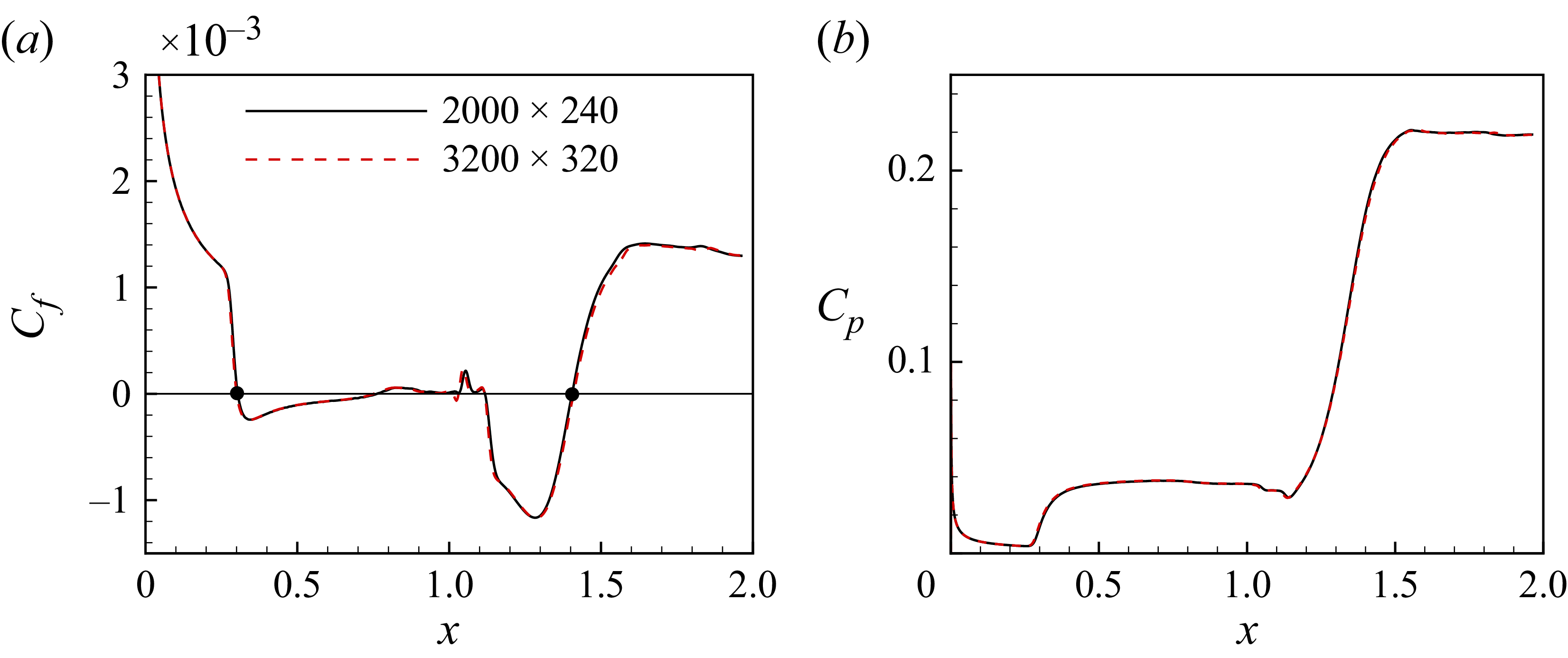
Because the transition to turbulence in a compression-ramp flow can be excited by the global instability, DNS are first performed in the absence of external disturbances. The 2-D base flow (laminar solution) is given in figure 1, where the numerical schlieren (density gradient contour) characterises the flow separation and reattachment as well as the shock system. Due to a large adverse pressure gradient induced by the shock, a remarkable separation bubble is produced around the corner. Figure 2 shows the streamwise distribution of skin friction coefficient
 $C_{\kern-1pt f}$
and surface pressure coefficient
 $C_{\kern-1pt p}$
for the base flow. Two mesh resolutions, i.e.
 $2000\times 240$
and
 $3200\times 320$
, are considered to illustrate grid independence. It can be measured from figure 2(a) that the separation point is located at
 $x = 0.30$
and the reattachment point at
 $x = 1.41$
. It is noted that secondary separation (Shvedchenko Reference Shvedchenko2009) occurs beneath the primary separation bubble at
 $x \approx 0.8{-}1$
and
 $x \approx 1.05{-}1.12$
. As a result, the primary bubble fragments into multiple vortices (see figure 1). This phenomenon is a sign of the existence of global instability (Hao et al. Reference Hao, Cao, Wen and Olivier2021).
Numerical schlieren (density gradient contour) of the compression-ramp flow (2-D solution). Flow from left to right. Red lines indicate the boundary of computational domain; the lower boundary corresponds to the wall. Blue lines indicate streamlines embedded in the separation bubble.

Streamwise distribution of (a) the skin friction coefficient and (b) the surface pressure coefficient for two mesh resolutions. The solid circles mark the separation and reattachment positions.

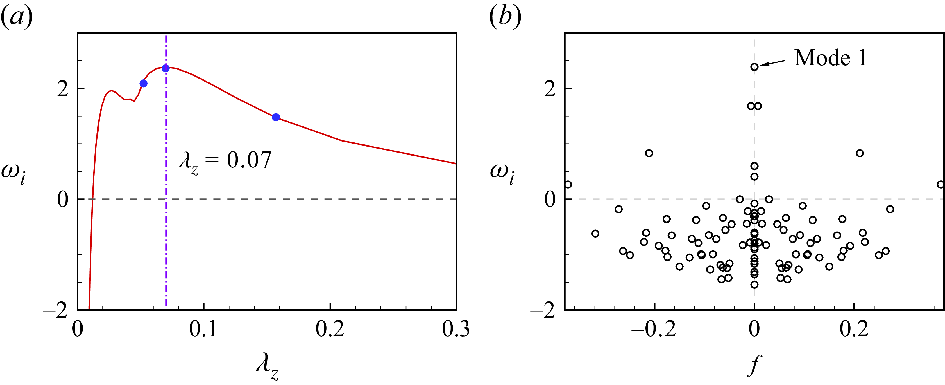
The GSA results. (a) Growth rate of the most unstable mode as a function of spanwise wavelength. Line indicates coarse mesh; solid circles indicate fine mesh. (b) Eigenvalue spectrum at
 $\lambda _z = 0.07$
.

Subsequently, GSA is performed to identify globally unstable modes in the base flow. Figure 3(a) plots the growth rate of the most unstable mode (mode 1) as a function of spanwise wavelength
 $\lambda _z$
. As seen in the figure, mode 1 is unstable in a wide range of
 $\lambda _z$
, and its growth rate peaks at
 $\lambda _z = 0.07$
with
 $\omega _i = 2.39$
. The corresponding eigenvalue spectrum at
 $\lambda _z = 0.07$
is shown in figure 3(b). Except for mode 1, there are five additional unstable modes, including two stationary modes and three oscillatory modes. The identified large growth rate and the presence of multiple unstable modes indicate that the global instability is quite strong. In this view, 3-D simulation is then carried out to explore the transition process associated with the global instability.
The initial 3-D flow field is built by extending the 2-D solution in the spanwise direction. At
 $t = 0$
, the simulation starts without introducing any artificial disturbances in the inflow or at the wall. To monitor the occurrence of three-dimensionality, the quadratic mean of the spanwise velocity
 $w$
at
 $x = 1.12$
, which is defined by
 \begin{align} A_w = \sqrt {\frac {1}{N_y N_z} \sum _{j=1}^{N_y} \sum _{k=1}^{N_z} w_{j,k}^2}, \end{align}
is considered. Here,
 $N_y$
and
 $N_z$
are the numbers of grid points in the
 $y$
and
 $z$
directions. The choice
 $x = 1.12$
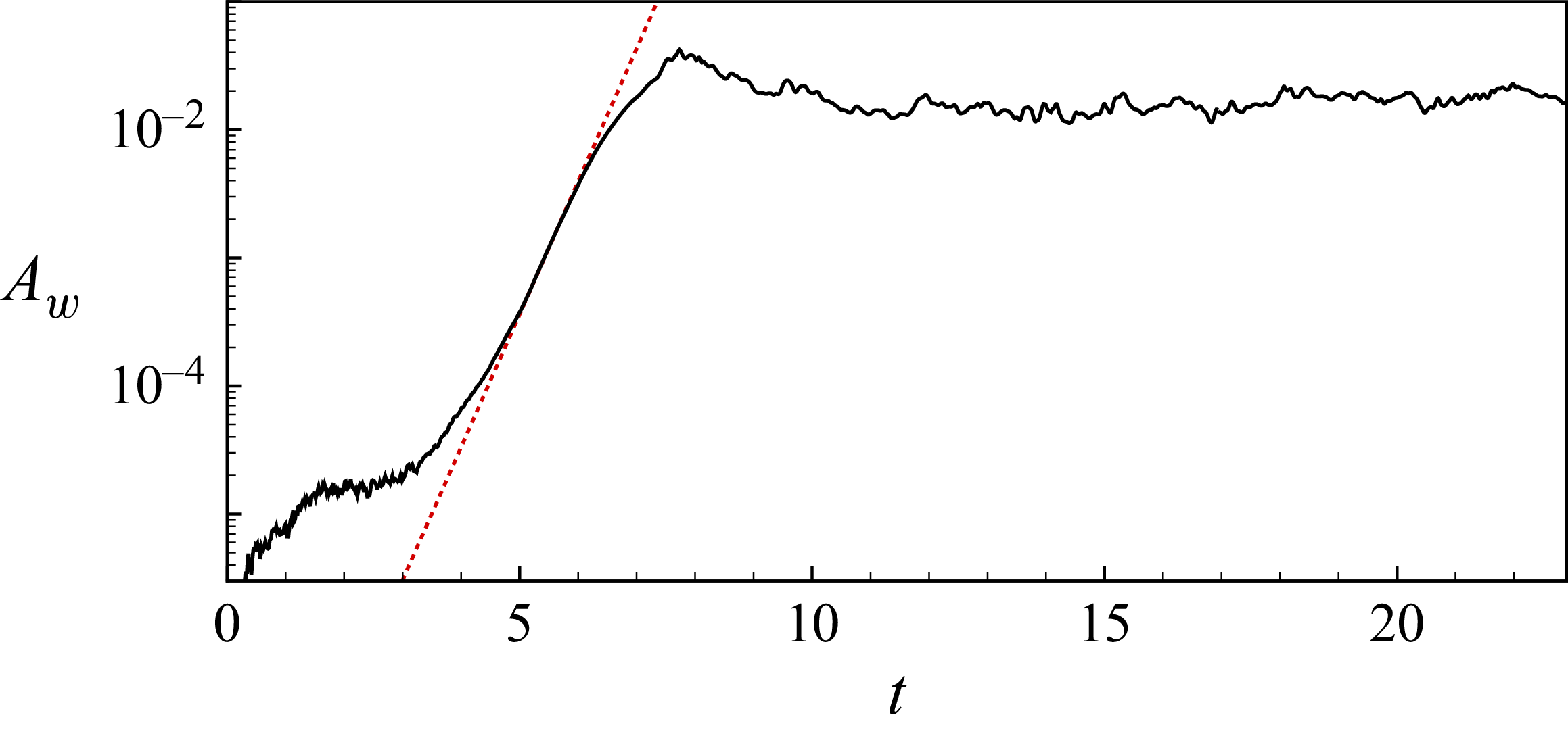
is based on the fact that the global instability emerges inside the separation bubble and is very strong near the recirculation core (Cao et al. Reference Cao, Hao, Klioutchnikov, Olivier and Wen2021). Figure 4 plots the temporal evolution of
 $A_w$
. After a transient process, it begins to grow exponentially. The growth rate matches the value predicted by the GSA (namely
 $\omega _i = 2.39$
). Subsequently, the unstable modes saturate, and
 $A_w$
reaches a quasi-steady state at approximately
 $t = 12$
, after which the flow is considered to be fully developed.
The detailed flow structure corresponding to
 $t = 21$
and 23 is presented in figure 5. Isolines of
 $C_{\kern-1pt f} = 0$
are shown on the wall to indicate the separation and reattachment regions. The
 $Q$
-criterion is used to visualise the vortical structures. The isosurface of
 $Q = 150$
is presented and coloured by the total velocity
 $U$
. Upstream of separation, the flow is clean as no external disturbances are introduced. Inside the separation bubble, the recirculating flow is rather irregular in the downstream part. At
 $t = 21$
, elongated streamwise streaks resulting from the global instability are visible downstream of reattachment. The transition to turbulence is found a certain distance downstream (close to the outflow boundary). At
 $t = 23$
, however, no distinct streamwise streaks are observed in the reattachment region, and the transition to turbulence takes place immediately downstream of reattachment. The instantaneous flows above suggest a long transition zone over the ramp. It seems that this transition process is slightly different from that described by Cao et al. (Reference Cao, Hao, Klioutchnikov, Wen, Olivier and Heufer2022), where the transition zone was short and was located far downstream of reattachment. To this end, we subsequently analyse the transition zone in the present flow.
3.2. The transition zone
Figure 6, where contours of streamwise momentum
 $\rho u$
are shown on a wall-parallel plane at
 $y_n = 0.0025$
, provides some evidence for the breakdown of streaks. At
 $t = 21$
, the streaks keep straight until approximately
 $x = 1.7$
. Then spanwise distortion appears as a result of secondary instability, which is followed by a quick breakdown to turbulence. At
 $t = 23$
, however, the spanwise distortion of streaks can be observed downstream of
 $x = 1.4$
, which is well upstream of that at
 $t = 21$
. Note that the spanwise-averaged reattachment point is located at
 $x = 1.39$
and 1.34 for
 $t = 21$
and 23, respectively.
Temporal evolution of the spanwise velocity (3.1) at
 $x = 1.12$
. The slope of the dotted line corresponds to the growth rate of mode 1 predicted by GSA.

Instantaneous flow field at (a)
 $t = 21$
and (b)
 $t = 23$
. Surface heat flux (Stanton number) together with isolines of
 $C_{\kern-1pt f} = 0$
are shown at the wall. The density gradient contour at
 $z = 0$
is shown to indicate the SBLI. The
 $Q$
-criterion (coloured by the total velocity
 $U = \sqrt {u^2 + v^2 + w^2}$
) is used to visualise the transitional and turbulent flows.

Contour of
 $\rho u$
on a wall-parallel plane (
 $y_n = 0.0025$
) at (a)
 $t = 21$
and (b)
 $t = 23$
. The spanwise-averaged reattachment point is located at
 $x = 1.39$
and 1.34 for
 $t = 21$
and 23, respectively.

Time history of streamwise velocity fluctuation at different streamwise locations on the centre plane (
 $z = 0.07$
). All positions are taken from a streamline passing through the shear layer over the separation bubble.

To better illustrate the intermittent transition process, figure 7 plots the time history of streamwise velocity fluctuation
 $u'$
in the flow field. The sampling positions are located on a streamline in the
 $x$
–
 $y$
plane at
 $z = 0.07$
, which passes through the shear layer over the separation bubble in the time- and spanwise-averaged flow. At
 $x = 1.2$
, the shear layer is almost undisturbed, which is consistent with the fact that the global instability occurs inside the separation bubble. At
 $x = 1.3$
, the reattaching shear layer exhibits low-frequency unsteadiness consistent with previous studies (Cao et al. Reference Cao, Hao, Klioutchnikov, Olivier and Wen2021, Reference Cao, Hao, Klioutchnikov, Wen, Olivier and Heufer2022). As expected, high-frequency components occur downstream of
 $x = 1.4$
in the reattached boundary layer, indicating the breakdown to turbulence.
Streamwise distribution of the skewness.

It should be mentioned that the increase in skin friction and surface heat flux as a result of transition is coupled with the flow reattachment (see below), which is similar to some flows in Fu et al. (Reference Fu, Karp, Bose, Moin and Urzay2021) and Cao et al. (Reference Cao, Hao and Guo2024). This makes it difficult to determine the transition onset from the distributions of skin friction and surface heat flux. Therefore, we consider the skewness of the streamwise velocity fluctuation to identify the exact position of transition onset. The skewness has been previously employed to determine the transition onset in boundary layers over a flat plate (Veerasamy & Atkin Reference Veerasamy and Atkin2020) and turbine blade (Gomes et al. Reference Gomes, Stotz, Blaim and Niehuis2015). Following Gomes et al. (Reference Gomes, Stotz, Blaim and Niehuis2015), the present skewness is defined as
 \begin{align} sk(u') = \left ( \frac {1}{N} \sum _{i=1}^{N} u'^3 \right ) \Bigg/ \left ( \frac {1}{N} \sum _{i=1}^{N} u'^2 \right )^{3/2}. \end{align}
Figure 8 shows the streamwise distribution of the skewness. As pointed out by Gomes et al. (Reference Gomes, Stotz, Blaim and Niehuis2015), the location of maximum skewness corresponds to the transition onset. It is therefore obvious that the transition onset in the present flow is located at
 $x = 1.41$
. This position is located downstream of the time- and spanwise-averaged reattachment point (
 $x = 1.36$
, see below). Thus it can be concluded that the transition zone in the compression-ramp flow without external disturbances is located downstream of reattachment, which proves our conjecture for the SLBLI. In this regard, many recent studies concerning the laminar–turbulent transition in SBLI belong to SLBLI, such as Fu et al. (Reference Fu, Karp, Bose, Moin and Urzay2021), Dwivedi et al. (Reference Dwivedi, Sidharth and Jovanović2022), Benitez et al. (Reference Benitez, Borg, Scholten, Paredes, McDaniel and Jewell2023b
) and Cao et al. (Reference Cao, Hao and Guo2024).
4. Transition to turbulence in the presence of strong disturbances
4.1. The complete transition process
The above transition scenario may be found in a low-disturbance environment, e.g. in a quiet tunnel. However, in a noisy environment, which is the case for many conventional wind tunnels, the transition scenario may differ. In the following, we first present the experimental results obtained in the JF8A. Then well-designed DNS are performed to reproduce the experiment. Finally, we examine the effects of disturbance amplitude on the transition process.
Figure 9 shows the schlieren image obtained in the experiment. An animation showing the flow establishment process is provided in the supplementary material are available at https://doi.org/10.1017/jfm.2026.11596. It can be seen that as the separation bubble grows, the separation point moves upstream and finally stops at
 $x = 0.6{-}0.7$
, and the reattachment point is located slightly downstream of the corner. In the fully developed flow, the reattached boundary layer appears to be in a turbulent state. It is obvious that the separation bubble is much smaller than the case in the absence of external disturbances (see figure 5). This discrepancy is attributed to the strong disturbances in the shock tunnel, which are visible in the animation.
Schlieren image obtained from experiment.

To numerically reproduce the compression-ramp flow in the experiment, we consider introducing disturbances that may occur in a noisy wind tunnel. It is well known that the dominant disturbances in a high-speed wind tunnel are acoustic disturbances that are radiated from the turbulent high-speed boundary layers along the nozzle walls (Laufer Reference Laufer1961; Schneider Reference Schneider2008; Duan et al. Reference Duan2019). In this view, FLDI is employed to measure the freestream disturbances in the JF8A. Figure 10 provides the power spectral density (PSD) of the freestream density disturbances measured at three different Reynolds numbers. The obtained spectra are similar to those reported by Duan et al. (Reference Duan2019). Note that while pressure fluctuations were measured directly by Duan et al. (Reference Duan2019), FLDI data can also interpret freestream pressure fluctuations quantitatively (Lawson et al. Reference Lawson, Neet, Hofferth and Austin2022). In the low- and high-frequency ranges, the spectra may be modelled by a constant-slope function, where the spectral slopes can be chosen as
 $-0.5$
and
 $-3.0$
, respectively.
Spectra of freestream density disturbances measured in the JF8A.

Recent work by Wagner et al. (Reference Wagner, Schülein, Petervari, Hannemann, Ali, Cerminara and Sandham2018) demonstrated that a slow acoustic wave is the dominant acoustic mode in noisy hypersonic wind tunnels. The slow acoustic wave model has been widely used to study the boundary layer transition in high-speed flows (Marineau Reference Marineau2017; Cerminara & Sandham Reference Cerminara and Sandham2020; Guo, Hao & Wen Reference Guo, Hao and Wen2025). Here, the freestream perturbation variable is defined as
 $\boldsymbol{\phi }'=(\rho ', u', v', w', p')^{\text{T}}$
. Taking the example of density disturbance, it is given by
 \begin{align} \rho '(x,z,t) = \varepsilon _\infty \sum _{m=1}^{M} \sum _{n=0}^{N} \rho '_{m,n}, \end{align}
where
 $\varepsilon _\infty$
controls the disturbance amplitude, and
 $\rho '_{m,n}$
represents the disturbance variable for a single Fourier mode
 $(m,n)$
, which is assumed as
 \begin{align} \rho '_{m,n} = A_m [\cos (\beta _n z + \psi _{m,n}) + \cos (-\beta _n z + \psi _{m,n})] \cos (\alpha _m x - \omega _m t + \varphi _m). \end{align}
Here, the subscripts
 $m$
and
 $n$
correspond to the
 $m$
th frequency and the
 $n$
th spanwise wavenumber,
 $\alpha$
and
 $\beta$
indicate the streamwise and spanwise wavenumbers,
 $\omega$
is the angular frequency, and
 $A_m$
controls the amplitude of the
 $m$
th component. The symbols
 $\psi _{m,n}$
and
 $\varphi _m$
represent randomly generated constant phase angles that do not change with time. It is noted that when
 $n=0$
,
 $\beta _n$
and
 $\psi _{m,n}$
are fixed at zero. Note also that
 $\omega _m = 2\pi f_m$
, where
 $f_m$
is the non-dimensional frequency. In (4.2), the streamwise wavenumber and the angular frequency are linked through the equation
 \begin{align} \alpha _m = \frac {\omega _m}{1 \pm 1/(M_\infty \cos \theta )}, \end{align}
where the
 $\pm$
sign indicates fast and slow acoustic waves, respectively. As mentioned previously, in this paper we consider the slow acoustic wave. In (4.3),
 $\theta$
denotes the oblique wave angle in the
 $x$
–
 $z$
plane and is given by
 $\theta _{m,n} = \arctan (\beta _n / \alpha _m)$
.
The total number of modes can be adjusted by varying
 $M$
and
 $N$
, which correspond to the number of frequencies and non-zero spanwise wavenumbers. In the present study, dimensional frequencies (
 $f^*_m$
) ranging from 10 kHz to 1000 kHz with interval 10 kHz are considered. As a result, 100 frequency components are included, i.e.
 $M = 100$
. This is reasonable according to the experimental measurements. In addition, the dimensional spanwise wavenumber ranges from 800 to 16 000
 $\text{m}^{-1}$
with interval 800
 $\text{m}^{-1}$
, leading to
 $N = 20$
. The corresponding spanwise wavelength varies from 0.39 to 7.9 mm.
In terms of amplitude, the model proposed by Balakumar & Chou (Reference Balakumar and Chou2018) is employed. This model evaluates the amplitude on the basis of the measured PSD of freestream pressure disturbances in Marineau et al. (Reference Marineau, Moraru, Lewis, Norris, Lafferty and Johnson2015). Here, the frequency-dependent amplitude
 $A_m$
is determined by
 \begin{align} A_m = \begin{cases} \sqrt {C_L f_m^{*-0.5}\, \Delta f^*/2}, & f_m^* \leqslant 100 \ \text{kHz}, \\[6pt] \sqrt {C_H f_m^{*-3}\, \Delta f^*/2}, & \text{otherwise}, \end{cases} \end{align}
where the constants in the low- and high-frequency parts are
 $C_L = 4 \times 10^{-7}$
and
 $C_H = 1.26 \times 10^6$
in SI units, which ensure a smooth transition from the low-frequency components to the high-frequency components. The laws of
 $f_m^{*-0.5}$
and
 $f_m^{*-3}$
are determined using the present experimental data (see figure 10) instead of those in Balakumar & Chou (Reference Balakumar and Chou2018). The resulting amplitude at
 $f_m^* = 100 \ \text{kHz}$
is
 $2.5 \times 10^{-3}$
for
 $\Delta f^* = 10$
kHz, which is comparable to the amplitude obtained by Balakumar & Chou (Reference Balakumar and Chou2018). As seen in (4.1), the final amplitude of a disturbance variable can be rescaled by
 $\varepsilon _\infty$
, which enables a parameter study for different amplitudes. In the present study,
 $\varepsilon _\infty = 0.5$
, 1 and 1.5 are considered to examine their influence on the transition process.
According to the dispersion relations that link the velocity, pressure and temperature perturbations to the density perturbation (Cerminara & Sandham Reference Cerminara and Sandham2020; Guo et al. Reference Guo, Hao and Wen2025), the disturbance for other variables is
 \begin{align} u'_{m,n} = - \frac {1}{M_\infty } \rho '_{m,n} \cos \theta _{m,n}, \quad v'_{m,n} = w'_{m,n} = 0, \quad p'_{m,n} = \gamma \rho '_{m,n}. \end{align}
Here,
 $\gamma$
denotes the specific heat ratio and is given by 1.4.
Time history of
 $u'$
(red line),
 $p'$
(green line) and
 $\rho '$
(blue line) at
 $x = 0$
for case
 $\varepsilon _\infty = 1$
.

Next, the above disturbance model is utilised in the DNS to investigate the transition scenario in the considered compression-ramp flow. Disturbances
 $\boldsymbol{\phi} '$
are introduced in the freestream at the beginning of simulation (i.e.
 $t=0$
). Note that we start 3-D simulations directly, rather than using the 2-D solution in § 3 as the initial flow field. The flow establishment process for case
 $\varepsilon _\infty = 1$
is demonstrated in the supplementary material using an animation. In addition, the fluctuation of density, velocity and pressure at the inlet (
 $x = 0$
) is monitored in figure 11. As expected, the velocity perturbation is much weaker than the pressure and density perturbations. The pressure perturbation has the largest amplitude. But the maximum is less than 0.08. The relatively small amplitude implies that the flow upstream of separation remains in the linear regime, which may explain why the boundary layer upstream of separation is in the laminar state.
Numerical schlieren of the compression-ramp flow in the presence of external disturbances with different amplitudes: (a)
 $\varepsilon _\infty = 0.5$
, (b)
 $\varepsilon _\infty = 1$
and (c)
 $\varepsilon _\infty = 1.5$
. The triangle marks the reattachment position in the time- and spanwise-averaged flows.

Figure 12 illustrates the numerical schlieren of the fully developed compression-ramp flows with
 $\varepsilon _\infty = 0.5$
, 1 and 1.5. For convenience, we label the four cases in §§ 3 and 4 as A0, A0.5, A1 and A1.5, where the number means the amplitude of disturbances. In the figure, the blue triangles mark the time- and spanwise-averaged reattachment point. It is obvious that in cases A0.5, A1 and A1.5, the separation bubble is much smaller than in case A0, and the transition to turbulence appears near the reattachment region. Additionally, the size of the separation bubble is sensitive to the disturbance amplitude. A larger amplitude causes a smaller separation bubble. This is due to an earlier transition induced by the large amplitude. Owing to the presence of strong disturbances, the boundary layer on the flat plate and the shear layer over the separation bubble are very unstable, indicating the effects of convective instabilities. This is discussed later.
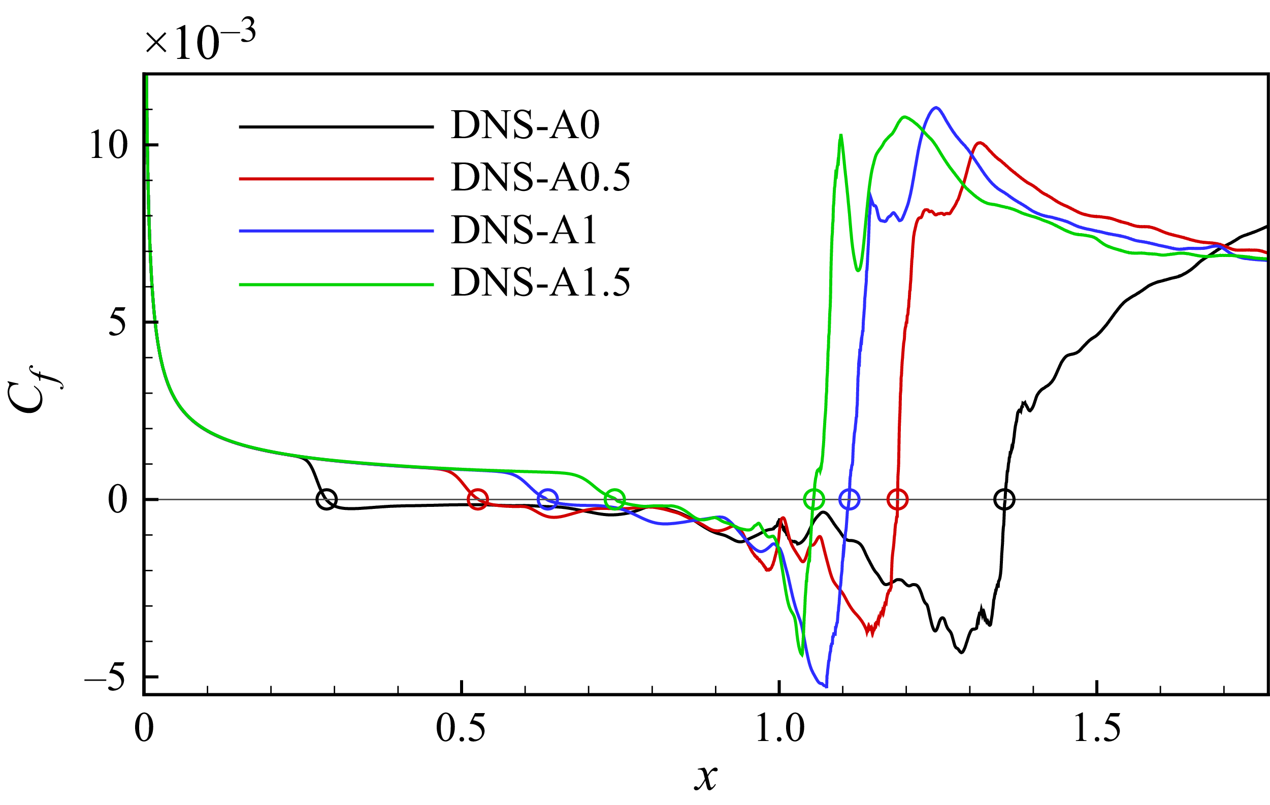
Streamwise distribution of the skin friction coefficient obtained from numerical simulations. The circles correspond to the separation and reattachment positions.

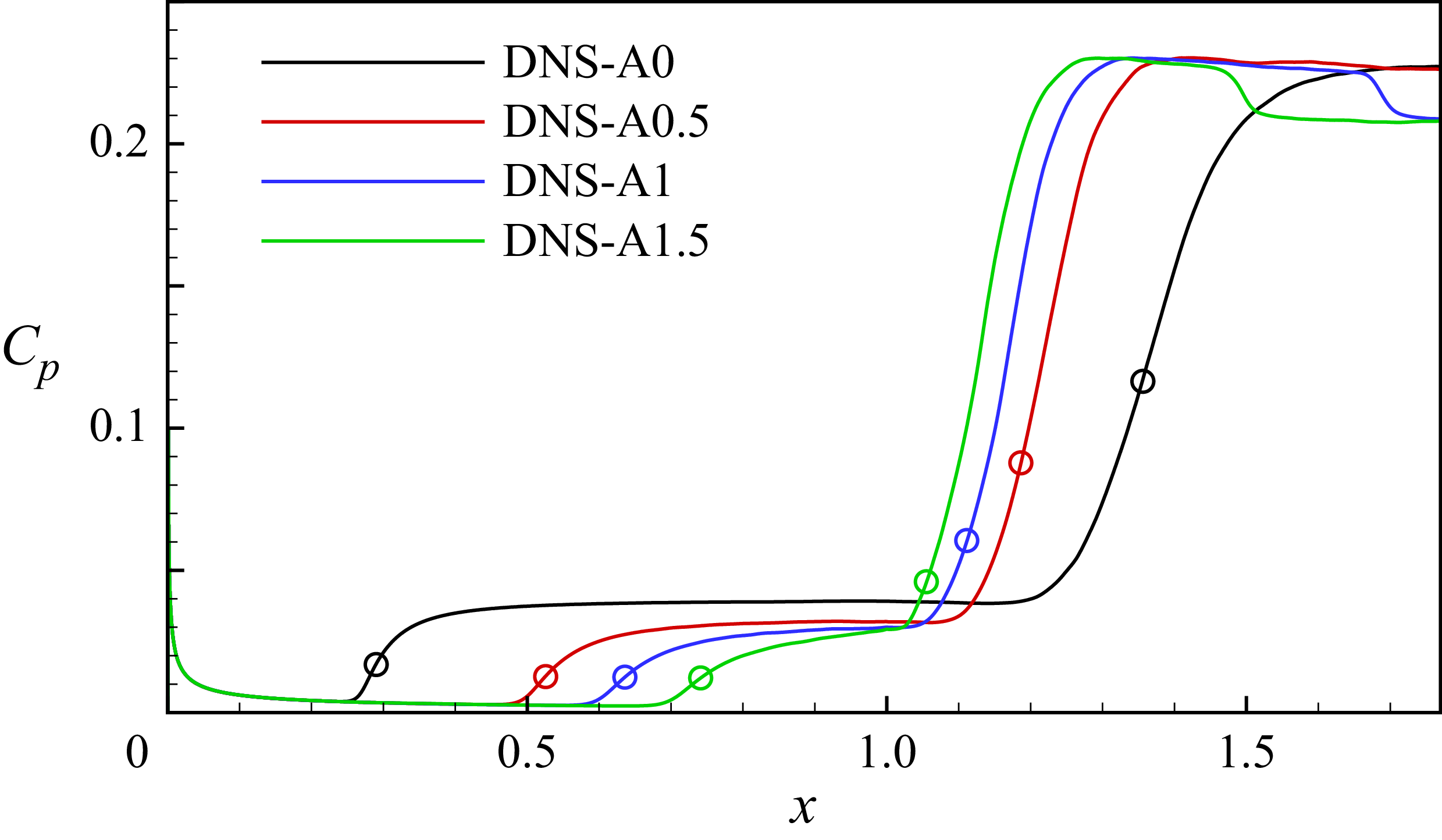
Streamwise distribution of the surface pressure coefficient obtained from numerical simulations. The circles correspond to the separation and reattachment positions.

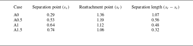
To facilitate a direct comparison between DNS and experiments, we plot the streamwise distribution of the skin friction coefficient, the surface pressure coefficient and the Stanton number in figures 13, 14 and 15, respectively. In these figures, all the DNS data are obtained from time- and spanwise-averaged flows. The decrease in the extent of the separation bubble with increasing disturbance amplitude is apparent in figure 13. It is easy to determine the separation and reattachment positions by finding the intersection between the data and
 $C_{\kern-1pt f} = 0$
. These points are highlighted by circles in the figure and are listed in table 2. The length of the separation bubble, which is defined by the difference between reattachment point
 $x_r$
and separation point
 $x_s$
, is also shown in the table. It is also seen that despite of the strong disturbances, the boundary layer upstream of separation is in a laminar state for all cases. Figure 14 shows typical surface pressure distribution for an SBLI. The pressure rise on the flat plate and the ramp highlights the separation shock and reattachment shock. Note that the pressure over the ramp will finally recover to the inviscid level after passing the expansion fan emanating from the triple point (Cao et al. Reference Cao, Hao, Klioutchnikov, Wen, Olivier and Heufer2022).
Time- and spanwise-averaged separation and reattachment points.

Streamwise distribution of the Stanton number obtained from experiments and numerical simulations. The circles correspond to the separation and reattachment positions.

Figure 15 gives the Stanton number data obtained from both the experiment and DNS. Here, the Stanton number is defined by
 $St = q_w^* / [\rho ^*_\infty U^*_\infty c_p (T^*_{aw} - T^*_w)]$
, where
 $q_w^*$
and
 $T^*_{aw}$
denote the wall heat flux and the adiabatic wall temperature. As shown in the figure, the extent of the separation bubble in case A0 is more than twice that in the experiment. Nevertheless, both the separation and reattachment positions in case A1 match well with the experimental results. Moreover, the laminar state of the boundary layer upstream of separation is also indicated by the experimental data, and far downstream of reattachment, both the experimental and numerical Stanton numbers approach the turbulent level.
Instantaneous flow field for case A1. Surface heat flux (Stanton number) together with isolines of
 $C_{\kern-1pt f} = 0$
are shown at the wall. The density gradient contour at
 $z = 0$
is shown to indicate the SBLI. The
 $Q$
-criterion (coloured by the total velocity
 $U = \sqrt {u^2 + v^2 + w^2}$
) is used to visualise the transitional and turbulent flows.

To visualise the transition process, an instantaneous flow field for case A1 is illustrated in figure 16. Similar to figure 5, the density gradient contour, the Stanton number contour and the
 $Q$
-criterion are employed. Upstream of separation, footprints of upstream disturbances are visible near the leading edge and on the wall. In the shear layer, the vortical structure reveals the evolution of instabilities. In the reattachment region, a rapid breakdown to turbulence is evident, and a fully turbulent boundary layer can be observed downstream. Next, we elaborate more on the instabilities that trigger this transition process.
In contrast to the transition scenario in § 3, the disturbances introduced in the present flows play a dominant role in destabilising the boundary layer and the shear layer, and promoting transition in the reattaching flow. To understand the convective instability, it is necessary to perform a normal-mode stability analysis for the upstream boundary layer. Under the same flow conditions, a new laminar flat-plate boundary layer is simulated with length 80 mm. The unstable mode is sought in a wide range
 $x\in [0.4, 0.8]$
,
 $\omega \in [0, 800]$
and
 $\beta \in [0, 1200]$
. Figure 17 displays the growth-rate contour of the most unstable mode at
 $x = 0.4$
. The growth-rate peak of the second mode is located at
 $(\omega , \beta )=(190,0)$
, while the growth-rate peak of the first mode is approximately located at
 $(\omega , \beta )=(40,90)$
. The corresponding dimensional frequencies of the most unstable second and first modes are approximately 319 and 67 kHz, respectively. The non-dimensional spanwise wavelength of the most unstable first mode is 0.07. At
 $x = 0.7$
, similar results are observed (contour not shown). While the frequency of the most unstable second mode shifts to 245 kHz due to a thickening of the boundary layer (Mack Reference Mack1984), the frequency of the most unstable first mode remains at 67 kHz. In addition, the spanwise wavelength of the most unstable first mode increases to 0.08.
Contour of the spatial growth rate
 $\sigma$
of the most unstable mode in the space
 $(\omega ,\beta)$
at the location
 $x = 0.4$
. Circles represent the most unstable oblique first and planar second modes.

The
 $N$
-factors for the first and second modes in the flat-plate boundary layer.

Spectra of the density fluctuation in the boundary layer (
 $x=0.4$
) and shear layer (
 $x=0.7$
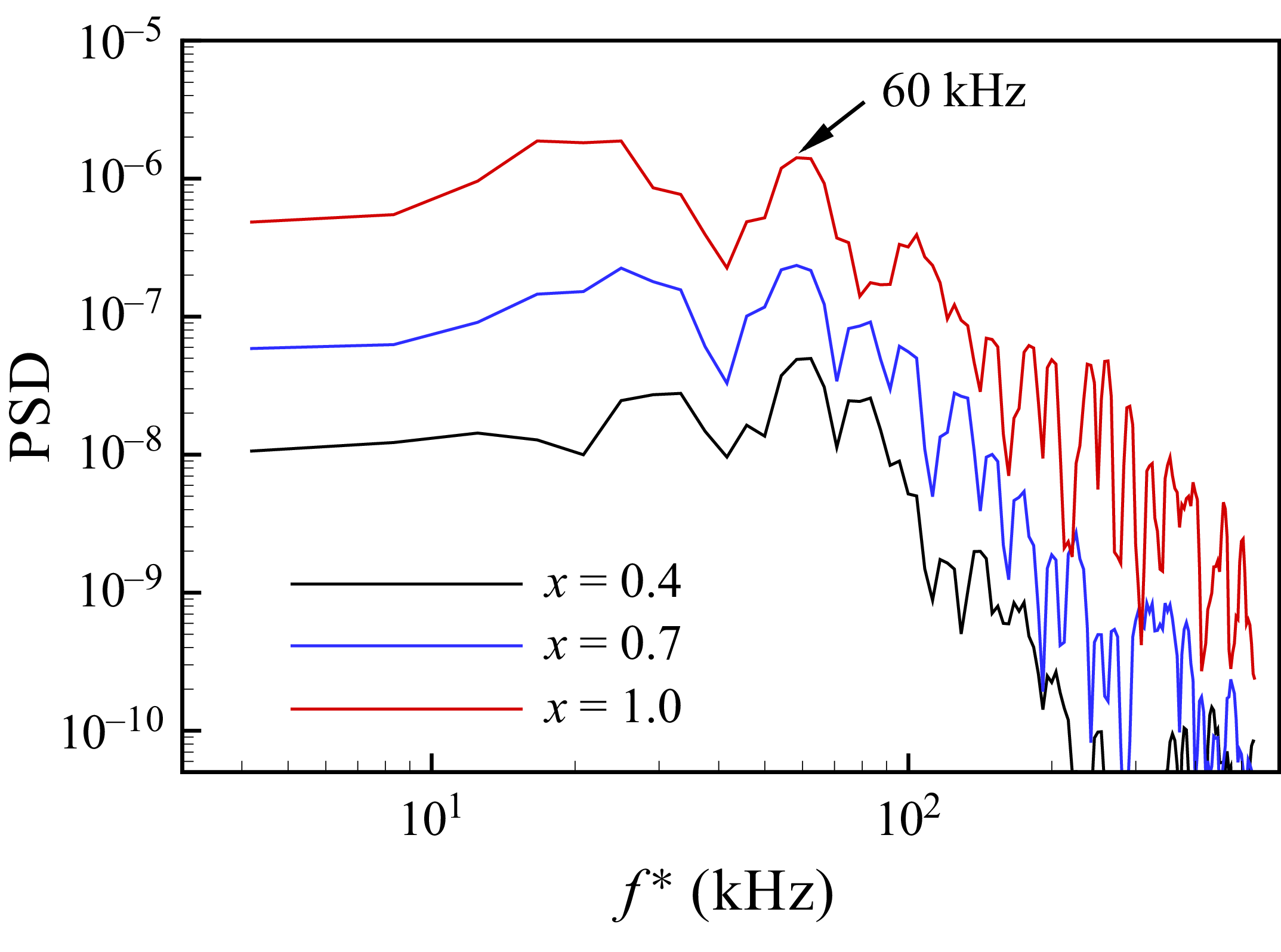
and 1.0) obtained from the DNS for case A1.

Then we carry out further analysis for the flat-plate boundary layer to illustrate the
 $N$
-factors for the first mode and second mode, which are shown in figure 18. Overall, the second mode exhibits a larger amplification rate than the first mode in the streamwise direction for most frequencies. Hence the second mode should dominate the disturbance growth if the initial amplitude for different frequency components is the same. However, in the experiment and DNS, the low-frequency disturbances have a much larger amplitude than the high-frequency disturbances (which is important for the second mode). As a result, the first mode becomes more significant than the second mode due to the large initial amplitude.
Towards this end, the spectra of the density fluctuation in the incoming boundary layer (at
 $x=0.4$
) and the shear layer for case A1 are given in figure 19. The two positions in the shear layer are
 $(x,y) = (0.7, 0.010)$
and
 $(1.0, 0.032)$
. As expected, the spectra are dominated by low frequencies due to the nature of the introduced disturbances. A local peak at approximately 60 kHz is evident at the three positions, which agrees well with the frequency of the most unstable first mode revealed by the local stability analysis for the upstream boundary layer. It indicates that the first mode originating from the upstream boundary layer is continuously amplified in the shear layer. Therefore, it is concluded that the first mode, as well as other low-frequency modes that originate from the upstream disturbances, finally promotes the transition to turbulence in the reattachment region.
4.2. The transition zone
It is clear that this transition scenario is different to that in § 3, as they are related to different instabilities. For cases A0.5, A1 and A1.5, the transition to turbulence is excited by the continuous forcing and is coupled with the flow reattachment process. To examine the transition zone, we first present the contour of
 $\rho u$
on a near-wall plane for case A1 in figure 20. Two time instants,
 $t = 22$
and 24, are considered. Note that a fully developed flow is established at
 $t \approx 14$
. Unlike case A0 (see figure 6), the two contours look very similar. In other words, there is no noticeable intermittency in the transition process for case A1. Furthermore, the rapid breakdown to turbulence is also apparent downstream of reattachment. The strong spanwise distortion at
 $x \approx 1.2$
suggests that it is in the late stage of breakdown. It should be emphasised that due to the spanwise distortion of the reattaching shear layer, the reattachment point ranges from
 $x = 1.07$
to
 $x = 1.17$
in the spanwise direction (see the blue triangles in the figure). Therefore, figure 20 mainly shows the boundary layer features downstream of reattachment, as the shear layer (upstream of
 $x = 1.17$
) is well above the wall (see figure 12).
Contour of
 $\rho u$
on a wall-parallel plane (
 $y_n = 0.0025$
) at (a)
 $t = 22$
and (b)
 $t = 24$
for case A1. The blue triangles mark the reattachment region, which ranges from
 $x = 1.07$
to
 $x=1.17$
.

Contour of streamwise velocity on the
 $y$
–
 $z$
plane at different
 $x$
positions for case A1, for (a)
 $t = 22$
and (b)
 $t = 24$
.

To demonstrate the distortion of the shear layer due to the convective instability, we show the contour of streamwise velocity on the
 $y$
–
 $z$
plane at different
 $x$
positions for case A1 in figure 21. At
 $x = 1.05$
, the shear layer, which is approximately located at
 $y_n = 0.15{-}0.02$
, exhibits spanwise periodicity in different scales. The largest spanwise scale has wavelength
 $\lambda _z = 0.08$
corresponding to the most unstable first mode discussed previously. Farther downstream (at
 $x = 1.1$
and 1.15), the reattaching shear layer is more distorted, and smaller streaks tend to be dominant. Downstream of reattachment (at
 $x = 1.2$
and 1.25), the spanwise periodicity breaks, and the tips of the low-speed streaks are quickly lifted up from the wall, indicating the final breakdown to turbulence (Mayer et al. Reference Mayer, Von Terzi and Fasel2011; Dwivedi et al. Reference Dwivedi, Sidharth and Jovanović2022).
Time history of streamwise velocity fluctuation at different streamwise locations on the centre plane (
 $x = 0.08$
) for case A1.

Subsequently, the time history of streamwise velocity fluctuation is plotted in figure 22 to provide more evidence for the transition zone. The sampling positions are taken from a streamline that passes through the shear layer and the reattached boundary layer on the centre plane (
 $z = 0.08$
). At
 $x = 1.05$
, the signal shows a strong periodicity, which is in line with the spatial periodicity in figure 21. However, the periodicity breaks at
 $x = 1.12$
, which is the time- and spanwise-averaged reattachment point (see table 2). As pointed out by Mayer et al. (Reference Mayer, Von Terzi and Fasel2011), the loss of periodicity is a sign for the final breakdown to turbulence. In addition, in the reattachment region at
 $x = 1.12$
and 1.15, higher frequencies appear in the signal, which also indicates the existence of secondary instability. Downstream of reattachment, the signal becomes more irregular, and finally approaches a typical distribution for a fully turbulent boundary layer (at
 $x = 1.7$
). As shown in Appendix, the boundary layer profile at
 $x = 1.25$
exhibits special features (e.g. several inflection points) for a transitional boundary layer, and the profile at
 $x = 1.75$
is typical of a turbulent boundary layer.
Although the breakdown to turbulence at reattachment has been observed in many experiments for STrBLI (e.g. Lugrin et al. Reference Lugrin, Nicolas, Severac, Tobeli, Beneddine, Garnier, Esquieu and Bur2022; Davami et al. Reference Davami2025; Threadgill et al. Reference Threadgill, Hader, Singh, Tsakagiannis, Fasel, Little, Lugrin, Bur, Chiapparino and Stemmer2025), the detailed flow features have not been clearly described before. Based on the above analyses, it is now clear that the flow remains in the transitional state in the whole reattachment region. In other words, a fully turbulent state is not reached in the reattaching flow, but the flow becomes fully turbulent a short distance downstream of the reattachment region, which presents more physical insights into STrBLI.
5. Discussion and conclusion
In this work, a compression-ramp flow at Mach 6.5 was studied using wind tunnel experiments, DNS and stability analyses. Two transition scenarios were revealed, which are linked to two groups of SBLI, i.e. SLBLI and STrBLI.
In the absence of external disturbances, the DNS capture the transition to turbulence downstream of reattachment. This transition scenario is initiated by the global instability in the separation bubble. Several unstable modes are identified by the GSA. The growth of the most unstable mode in the DNS is well predicted. In the fully developed flow, the unstable separation bubble continuously excites the transition process without the aid of external disturbances. The transition to turbulence in this flow exhibits strong intermittency. By examining the skewness of the streamwise velocity fluctuation, it was found that the transition onset is located downstream of the reattachment region.
In the experiment, however, owing to the strong freestream disturbances in the shock tunnel, a relatively small separation bubble forms at the corner. This flow deviates significantly from the compression-ramp flow without external disturbances. To numerically reproduce the experimental flow, slow acoustic waves that represent typical disturbances in a conventional supersonic wind tunnel were added to the freestream of DNS. The disturbance spectra were constructed on the basis of the FLDI measurement. Consequently, the DNS capture the transition to turbulence in the vicinity of the reattachment region. With an appropriate amplitude of disturbances, both the separation bubble size and the surface heat flux distribution match well with the experimental data. By performing local stability analysis for the upstream boundary layer, it was found that the growth rate of the most unstable first mode peaks at 67 kHz. The spectra of the shear layer fluctuations in the DNS also exhibit a local peak at 60 kHz, indicating a prominent role of the first mode. In short, this transition scenario is excited by the strong external disturbances, and the final transition to turbulence is provoked by the convective instability. Concerning the detailed flow behaviour in the transition zone, it is shown that the reattaching shear layer is transitional, and the reattached boundary layer breaks down to turbulence a short distance downstream of reattachment. In other words, the reattachment region is completely situated inside the transition zone.
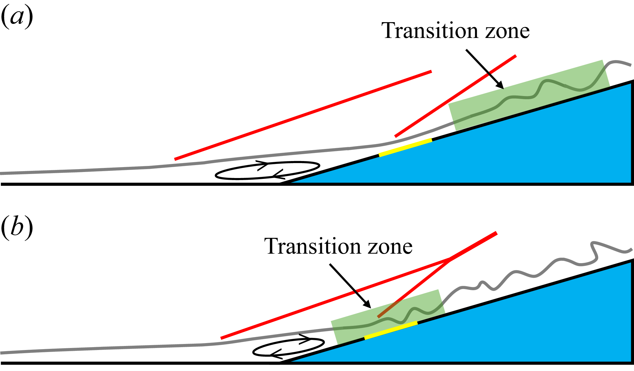
Schematic transition zone for (a) SLBLI and (b) STrBLI over a compression ramp. Red lines indicate shock waves. Yellow lines indicate the reattachment region.

According to the present study, it is appropriate to propose the following criteria to distinguish between SLBLI and STrBLI in the framework of laminar–turbulent transition (see also figure 23). In an SLBLI, the transition zone, namely, the region covered by the transition onset and end, is located downstream of the reattachment region. In our previous work (Cao et al. Reference Cao, Hao, Klioutchnikov, Wen, Olivier and Heufer2022, Reference Cao, Hao and Guo2024; Huang et al. Reference Huang, Cao, Hao, Guo and Wen2025a ) and many other studies (Fu et al. Reference Fu, Karp, Bose, Moin and Urzay2021; Dwivedi et al. Reference Dwivedi, Sidharth and Jovanović2022; Benitez et al. Reference Benitez, Borg, Scholten, Paredes, McDaniel and Jewell2023b ), the transition zone is located either close to the reattachment region or well downstream of reattachment. These are important characteristics of SLBLI. More importantly, in these studies, the separation bubble size is nearly not influenced by the transition process. This is the other prominent feature of SLBLI. It is reasonable because the reattachment region is located upstream of the transition zone, thus the reattaching shear layer is still in the laminar state.
On the other hand, both the reattaching shear layer and the reattached boundary layer in the vicinity of reattachment become highly transitional, as the reattachment region in an STrBLI is well covered by the transition zone. It is known that a transitional boundary layer has a greater resistance to adverse pressure gradient. This explains why the separation bubble shrinks in an STrBLI. In fact, the shrinking of the separation bubble is commonly observed in experiments with strong freestream disturbances (e.g. Currao et al. Reference Currao, Choudhury, Gai, Neely and Buttsworth2020; Lugrin et al. Reference Lugrin, Nicolas, Severac, Tobeli, Beneddine, Garnier, Esquieu and Bur2022; Davami et al. Reference Davami2025; Threadgill et al. Reference Threadgill, Hader, Singh, Tsakagiannis, Fasel, Little, Lugrin, Bur, Chiapparino and Stemmer2025). It is emphasised again that a fully turbulent state is not reached in the reattachment region, which is less noticed in the literature. One may conceive that if the reattaching flow becomes turbulent, then the SBLI tends to be an STBLI, and the separation bubble will be very small or even disappear.
In summary, the physics underlying the change of separation bubble size between SLBLI and STrBLI lies in the relative position between the reattachment region and the transition zone. Examining their relative positions allows us to identify whether a flow belongs to SLBLI or STrBLI. This contributes to building a comprehensive framework for SBLI.
Supplementary movies
Supplementary movies are available at https://doi.org/10.1017/jfm.2026.11596.
Funding
This research is supported by the National Natural Science Foundation of China (no. 12232018) and the Strategic Priority Research Programme of the Chinese Academy of Sciences (no. XDB 0620203).
Declaration of interests
The authors report no conflict of interest.
Appendix. Boundary layer profile
Figure 24 shows the boundary layer profiles obtained from the time- and spanwise-averaged flow for case A1. The streamwise velocity is transformed using van Driest transformation as the flow is compressible. The linear-sublayer and log-law relations are
 $u^+ = y^+$
,
 $u^+ = 2.5 \ln(y^+) + 5.8$
. As seen in the figure, the velocity profile at
 $x = 0.55$
manifests a laminar boundary layer. Note that its deviation from the linear-sublayer relation is due to the cold wall effects (Duan, Beekman & Martin Reference Duan, Beekman and Martin2010; Cao et al. Reference Cao, Hao, Klioutchnikov, Wen, Olivier and Heufer2022). At
 $x = 1.25$
, the profile has several inflection points, which is typical of a transitional boundary layer. At
 $x = 1.75$
, the profile indicates that a fully turbulent boundary layer is developed.
The van-Driest-transformed mean velocity profile at three
 $x$
positions for case A1. The dashed lines represent the linear-sublayer and log-law relations.