






1. Introduction
The flow-induced vibration (FIV) of closely placed cylinders significantly differs from that of an isolated cylinder. Many engineering applications such as buildings, heat exchanger tubes, offshore wind turbines, bridge pipelines, etc., often only exist as isolated systems. Further complexity in the system arises when these multibody systems are coupled through structural linkages. Some common examples are an overbridge between buildings, structural connections between parallel tubes and pipelines, connected offshore wind turbines, and twin bridge connections. Based on the structural coupling, these systems are accurately modelled as a rigidly or elastically coupled multistructure system placed in a cross-flow. Therefore, the present work focuses on studying the FIV response of an elastically coupled multicylinder system. A canonical set-up for studying multibody dynamics in a flow is two circular cylinders arranged in tandem (along the flow), side-by-side (transverse to the flow) and a staggered (diagonal to the flow) arrangement. Here, we focus on two circular cylinders in a tandem arrangement, vibrating only in the transverse direction. We briefly review the studies on circular cylinders with increasing complexity in the following subsections.
1.1. Studies on flow past an isolated cylinder
Extensive research has been carried out for flow past stationary circular cylinders (Zdravkovich Reference Zdravkovich1988; Williamson Reference Williamson1996b), rectangular plates (Matsumoto Reference Matsumoto1999), effects of systematic cross-section variation of the cylinders (Thompson et al. Reference Thompson, Radi, Rao, Sheridan and Hourigan2014; Sharma, Pandey & Bhardwaj Reference Sharma, Pandey and Bhardwaj2022b), etc. As highlighted by Williamson & Roshko (Reference Williamson and Roshko1988), a significant variation in wake structures occurs due to cylinder vibrations. Many researchers have extensively studied the FIV of the elastically mounted isolated cylinder and summarized earlier by Bearman (Reference Bearman1984), Rockwell (Reference Rockwell1998), Williamson & Govardhan (Reference Williamson and Govardhan2004), Sarpkaya (Reference Sarpkaya2004) and Mannini, Marra & Bartoli (Reference Mannini, Marra and Bartoli2014). Govardhan & Williamson (Reference Govardhan and Williamson2000) observed a high amplitude upper branch and relatively low amplitude lower branch synchronized FIV or lock-in and associated them with switching of the vortex and total force phases from  $0^\circ$ to
 $180 ^\circ$, respectively. While observations of Govardhan & Williamson (Reference Govardhan and Williamson2000) correspond to higher
 $Re~({\sim }3700)$, Leontini, Thompson & Hourigan (Reference Leontini, Thompson and Hourigan2006) observed a qualitatively similar FIV behaviour at low
 $Re$ of
 $200$. This qualitative similarity also extends to the non-circular cross-sections like a D-section (Zhao, Hourigan & Thompson Reference Zhao, Hourigan and Thompson2018; Sharma, Garg & Bhardwaj Reference Sharma, Garg and Bhardwaj2022a).
1.2. Two stationary cylinders in tandem arrangement
A stationary single cylinder placed in a cross-flow undergoes steady vortex shedding for a wide range of  $Re \in [150,4000]$ (Williamson Reference Williamson1996a), with nearly constant Strouhal number
 $St_{0} \sim 0.2$ and a periodic lift forcing. However, multiple stationary cylinders can result in a spectrum of responses, depending on the cylinder gap ratio, relative size and effective Reynolds number. At a given
 $Re$, the Strouhal number of the tandem cylinders (
 $St_{00}$) shows a continuous variation with cylinder centre-to-centre gap ratio
 $G$ (Igarashi Reference Igarashi1981; Xu & Zhou Reference Xu and Zhou2004; Zhou et al. Reference Zhou, Feng, Alam and Bai2009; Alam Reference Alam2014), especially at small
 $G$. The interaction between the two cylinders in stationary configurations has been investigated in various studies and summarized by Sumner (Reference Sumner2010) and Zhou & Alam (Reference Zhou and Alam2016).
With respect to the tandem cylinder configuration, Zdravkovich (Reference Zdravkovich1988) classified the flow as a proximity-wake interference regime for  $G<3.8$ and a wake interference regime for
 $G>3.8$. The proximity-wake interference regime is further subdivided into configurations where shear layers from the upstream cylinder (UC) directly form vortices (
 $G< 1.2$), steadily reattach to the downstream cylinder (DC) (
 $1.2< G<1.8$) or intermittently reattach to the DC (
 $1.8< G<3.8$). Similarly, Sumner (Reference Sumner2010) classified the system as single bluff body (
 $1< G<1.125$), shear layer reattachment (
 $1.125< G<4$) and vortex impingement (
 $G>4$), based on the resulting flow patterns. Hu & Zhou (Reference Hu and Zhou2008) also classified the stationary tandem cylinder configurations based on the flow structures as single street vortex shedding of type 1 and type 2, based on whether the downstream vortex strength is stronger or weaker than the isolated cylinder case, respectively.
Earlier studies primarily focused on the flow field around the cylinder. Very few studies considered other contributing factors, like the phase difference between the lift force on the two cylinders ( $\phi _{C_{L12}}$) and its effects on the wake characteristics. Sakamoto, Hainu & Obata (Reference Sakamoto, Hainu and Obata1987) studied flow past tandem square cylinders at
 $Re \sim O(10^4)$ and observed a linear increase in
 $\phi _{C_{L12}}$. They further reported that the onset of the coshedding regime, at a critical gap ratio
 $G_c$, is marked by
 $\phi _{C_{L12}} \sim 0^\circ$. Alam et al. (Reference Alam, Moriya, Takai and Sakamoto2003) observed a similar
 $\phi _{C_{L12}} \sim 0^\circ$ at the onset of coshedding (
 $G_c \sim 4$) for tandem circular cylinders at
 $Re=6.5 \times 10^4$. Similar to the high
 $Re$ studies, Alam (Reference Alam2016) also observed
 $\phi _{C_{T12}} \sim 0^\circ$ at
 $G_c \sim 3.5$ for
 $Re=200$. Therefore, the critical gap ratio
 $G_c$ is always accompanied by
 $\phi _{C_{T12}} \sim 0^\circ$ irrespective of the shape of the cylinders or the
 $Re$ of flow.
Alam et al. (Reference Alam, Moriya, Takai and Sakamoto2003) observed a local maxima of lift with increasing  $G$ for
 $\phi _{C_{L12}} \sim 2 n {\rm \pi}$ or
 $0^{\circ }$ and local minima of lift for
 $\phi _{C_{L12}} \sim (2 n+1) {\rm \pi}$ or
 $180^{\circ }$, and associated it with the in-phase and out-of-phase vortex shedding of the two cylinders. Alam (Reference Alam2016) further highlighted that a higher free stream flow into the wake of UC occurs with increasing
 $G$, further enhanced by the in-phase vortex shedding. Further, Wang, Alam & Zhou (Reference Wang, Alam and Zhou2018) investigated the flow past two tandem cylinders of unequal diameters at
 $Re=4.27 \times 10^4$ and observed that the vortex formation length of the UC primarily governs
 $G_c$.
1.3. Two tandem cylinders with one of them elastically mounted
The FIV of elastically mounted, either one or both of the tandem cylinders, has been extensively studied (Chen Reference Chen1986; Price Reference Price1995; Bearman Reference Bearman2011). One of the extensively studied tandem cylinder configurations constitutes the FIV of an elastically mounted cylinder placed in the wake of an upstream stationary cylinder (proximity-wake or wake interference (Zdravkovich Reference Zdravkovich1988)).
Past studies have analysed this system and identified various typical FIV regimes. Bokaian & Geoola (Reference Bokaian and Geoola1984b) studied this system using tandem cylinders with  $m \zeta = 0.019$ for
 $G \in [1.09,5]$ at
 $Re \sim 5600$, and identified four variations of the FIV response: galloping only (
 $G = 1.09$); combined vortex excitation and galloping (
 $G = 1.5$); separated vortex excitation and galloping (
 $G \in [2,3]$); and vortex excitation only (
 $G > 3$). Later, Assi, Bearman & Meneghini (Reference Assi, Bearman and Meneghini2010) reported a growing amplitude of vibrations extending for
 $G<8$ using cylinders of
 $m \zeta \sim 0.018$ at a higher
 $Re ({\sim }O(10^4)$) flow. However, they observed that the mechanism is not similar to single cylinder galloping, and termed it as wake-induced vibration (WIV). While the FIV regimes are similar at small
 $m \zeta$, higher
 $m \zeta$ show some deviations. Qin, Alam & Zhou (Reference Qin, Alam and Zhou2017) studied the
 $m \zeta = 0.58$ system at
 $Re \sim O(10^4)$ for
 $G \in [1.5,6]$ and observed no galloping-like WIV for equal diameter cylinders at any
 $G$. However, as they reduced the UC diameter, the downstream cylinder amplitude increased rapidly with
 $U_R$. Contrary to the classical single-cylinder galloping, they reported that galloping vibration during WIV is sustained by gap flow switching. Hu, Wang & Sun (Reference Hu, Wang and Sun2020b) further studied the effect of
 $m \zeta$ (
 $\in [184,0.719]$) and
 $G$ (
 $\in [1.1,8]$) on WIV response at
 $Re \sim O(10^4)$. They also observed a transition from galloping, to combined vortex excitation and galloping, to separated vortex excitation and galloping, to only vortex excitation, with increasing
 $m \zeta$ and
 $G$.
Notably, Assi et al. (Reference Assi, Bearman and Meneghini2010) observed a steadily increasing vibration frequency of the DC at high  $U_R$, which was not along the Strouhal frequency (
 $St_0 \sim 0.2$) or structural natural frequency (
 $f_n$). Hu, Wang & Sun (Reference Hu, Wang and Sun2020a) also observed a similar intermediate vortex shedding frequency between
 $St_0$ and
 $f_n$. Assi et al. (Reference Assi, Bearman, Carmo, Meneghini, Sherwin and Willden2013) cited this response as a result of wake-induced stiffness, dominant at high
 $U_R$, which controls the structural vibration frequency. Interestingly, Qin et al. (Reference Qin, Alam and Zhou2017) observed a significant reduction in vortex shedding frequency for smaller
 $G$ at high
 $U_R$, corresponding to the shear layer reattachment regime of stationary tandem cylinders (Zdravkovich Reference Zdravkovich1988). As pointed out in § 1.2,
 $St_{00}$, corresponding to tandem configuration, shows significant deviation from
 $St_0$. Therefore,
 $St_{00}$ can better quantify the FIV spectral characteristics.
As opposed to the former system, the upstream elastically mounted cylinder can also be placed in the proximity of a stationary downstream cylinder (proximity interference (Zdravkovich Reference Zdravkovich1988)). Bokaian & Geoola (Reference Bokaian and Geoola1984a) studied the FIV of an upstream cylinder for varying  $G \in [1.09,5]$ at
 $Re = 5900$ and
 $m \zeta = 0.019$. The UC shows galloping vibrations for
 $G<1.75$ and vortex-induced vibration (VIV) for
 $G \geq 2$. They also reported a shift in the mean position of the UC for small
 $G$ galloping vibrations. Similarly, Kim et al. (Reference Kim, Alam, Sakamoto and Zhou2009) also observed galloping vibrations of the UC at
 $G = 1.3$ and small amplitude VIV at
 $G = 4.2$ at
 $Re \sim O(10^4)$ and
 $m \zeta \sim 6$. Interestingly, they reported a suppression in FIV for a narrow region around
 $G = 2.2$ between the galloping and VIV excitation.
1.4. Two tandem cylinders with both being elastically mounted
Experimental findings of Kim et al. (Reference Kim, Alam, Sakamoto and Zhou2009) show that the cylinders, which show negligible vibration amplitudes near a stationary cylinder, may undergo high amplitude vibrations if the other cylinder is also elastically mounted. King & Johns (Reference King and Johns1976) observed FIV characteristics of two tandem cylinders at  $Re \sim O(10^4)$ for
 $G \in [2.25,7]$, and reported two variations of vortex lock-in regimes at all
 $G$: stronger vibrations of the UC (
 $A_1>A_2$) at lower
 $U_R$ and stronger vibrations of the DC (
 $A_2>A_1$) at higher
 $U_R$, followed by galloping at small
 $G$. Using cylinders of
 $m \zeta = 6.36$ at
 $G \in [1.1, 4.2]$ placed in an
 $Re \sim O(10^4)$ flow, Kim et al. (Reference Kim, Alam, Sakamoto and Zhou2009) observed five different regimes: no vibration (
 $G = 1.1$); vibrations dominated by upstream cylinder (
 $G = [1.2,1.6)$); vibration response dominated by downstream cylinder (
 $G \in [1.6,3.0)$); small vibration with wake reattachment (
 $G \in [3.0, 3.7)$); and wake induced vibrations (
 $G \geq 3.7$). Qin, Alam & Zhou (Reference Qin, Alam and Zhou2019) reported strong galloping vibrations with
 $A_1>A_2$ at
 $G \leq 1.5$, corresponding to
 $m \zeta =0.58$ an order of magnitude less than Kim et al. (Reference Kim, Alam, Sakamoto and Zhou2009). However, the galloping vibrations were suppressed when the UC was stationary. Further, they observed
 $A_1>A_2$ for VIV and low
 $U_R$ galloping, and
 $A_2>A_1$ for high
 $U_R$ galloping at
 $G \in (1.5,2.5)$. They observed strong dependence of the cylinder vibrations on the adjacent cylinder (stationary/vibrating) for
 $G \in [2.5,3]$, with this effect vanishing for
 $G>3$. Using the wake frequency modifications from the UC motion during the lock-in, Lin et al. (Reference Lin, Wang, Zheng and Sun2020) observed that
 $A_2$ at
 $m \zeta =0.018$, has negligible dependence on the frequency of upstream wake at
 $G = 4$ and
 $Re \sim O(10^3)$. However, a gradual increase in
 $A_2$ is observed with an increase in
 $Re$. Similar to § 1.3, Hu et al. (Reference Hu, Wang and Sun2020a) observed a transition from combined vortex shedding and galloping to separated vortex shedding and galloping, with increasing
 $G$ and
 $m \zeta$ at
 $Re \sim O(10^4)$.
The overall FIV response of tandem cylinders, with  $A_1 > A_2$ at low
 $U_R$ and
 $A_2 > A_1$ at high
 $U_R$, is also observed in the low
 $Re$ studies (Borazjani & Sotiropoulos Reference Borazjani and Sotiropoulos2009; Prasanth & Mittal Reference Prasanth and Mittal2009; Chung Reference Chung2017; Griffith et al. Reference Griffith, Jacono, Sheridan and Leontini2017). Using two-degree-of-freedom (2-DOF) (transverse and longitudinal) FIV of tandem cylinders (
 $m = 10, \zeta = 0.01$) for
 $G \in [2.5, 5]$ in an
 $Re = 160$ flow, Papaioannou et al. (Reference Papaioannou, Yue, Triantafyllou and Karniadakis2008) observed a delayed lock-in for a narrow range of
 $U_R$ with increasing
 $G$. This is caused due to the change in the corresponding tandem cylinder Strouhal frequency
 $St_{00}$, as vortex shedding frequency at
 $G = 2.5$ is close to the corresponding
 $St_{00}$ during desynchronization. Therefore,
 $St_{00}$ is better suited for FIV analysis of tandem cylinders. Borazjani & Sotiropoulos (Reference Borazjani and Sotiropoulos2009) studied FIV of one-degree-of-freedom (1-DOF) (transverse) and 2-DOF (transverse and longitudinal) vibration of tandem cylinders with
 $m = 2$ and
 $G = 1.5$ at
 $Re = 200$, and observed a wider lock-in range of
 $U_R$ for the 1-DOF case. The gap between the cylinders was reduced to
 $G = 1.2$ in the 2-DOF case, and the relative motion transformed into in-phase vibrations. This shows that
 $G$ and relative motion between the cylinders strongly influence the final FIV response. Prasanth & Mittal (Reference Prasanth and Mittal2009) (2-DOF,
 $m=10$,
 $G = 5.5$,
 $Re=100$) quantified the phase difference between the displacement of the two cylinders (
 $\phi _{y12}$) and observed a sharp jump in
 $\phi _{y12}$ during the transition from the
 $A_1 > A_2$ to the
 $A_2 > A_1$ regime, accompanied by
 $St_{00} \sim f_n$. Griffith et al. (Reference Griffith, Jacono, Sheridan and Leontini2017) (1-DOF,
 $m=2.546$,
 $G = 1.5$,
 $Re=200$) observed a
 $2S$ (two single vortices downstream) vortex shedding pattern for
 $A_1>A_2$, and a
 $2P$ (2 pair of vortices downstream) pattern for
 $A_2>A_1$ regime. However, Chung (Reference Chung2017) (2-DOF,
 $m=2$,
 $G \in [1.1,1.9]$,
 $Re = 100$) argued that the
 $2P$ pattern in near wake was observed due to gap flow and not due to cylinder vibrations, corresponding to single cylinder FIV. Further, they observed that the regime transitions shifted to higher
 $U_R$ at lower
 $Re$. Chen et al. (Reference Chen, Ji, Williams, Xu, Yang and Cui2018) studied the 1-DOF FIV of three tandem cylinders at
 $m = 2$ for uniform
 $G \in [1.2,5]$ at
 $Re=100$ and observed similar amplitude variations. The UC had a larger amplitude at lower
 $U_R$, and the DC had a larger amplitude at higher
 $U_R$ for
 $G > 1.5$. Similar to FIV of high
 $Re$ tandem cylinders, they observed galloping for all three cylinders at
 $G \leq 1.5$ and outlined three primary requirements: perfectly timed cylinder motion with vortex shedding; shift in the mean position; and high
 $U_R$.
1.5. Two elastically mounted coupled tandem cylinders
While the FIV of tandem cylinders discussed earlier is mainly influenced by coupling through the fluid, an additional mechanical coupling brings further complexity. In one of the earlier studies, King & Johns (Reference King and Johns1976) observed a delayed vibration response for an in-phase motion of elastically coupled tandem cylinders at  $G = 2$. Further, Price & Abdallah (Reference Price and Abdallah1990) modelled the 2-DOF tandem cylinder system using elastic coupling between them and proposed a frequency detuning technique for undamped FIV suppression. Brika & Laneville (Reference Brika and Laneville1997) investigated the in-phase and out-of-phase motion (controlled through mechanical linkages) FIV of tandem cylinders with
 $m \zeta \sim 0.08$ for a gap ratio of
 $25$ in an
 $Re \sim O(10^4)$ flow. They observed that matching (opposing) the intercylinder vibration phase
 $\phi _{y12}$ of a coupled system with the uncoupled tandem cylinder counterpart leads to a strong (suppressed) FIV response. Laneville & Brika (Reference Laneville and Brika1999) extended this study for smaller gap ratios
 $G \in [7,25]$ and observed a further increase in coupling effects with a reduction in
 $G$. Further, as the mechanical linkages were rigid, the amplitude of the coupled cylinders in favourable
 $\phi _{y12}$ conditions was identical (
 $A_1=A_2$) and close to the mean of FIV amplitudes of the two cylinders in an independent configuration. Therefore, even if
 $\phi _{y12}$ is favourable for FIV, the elastic coupling between the cylinders also controls the preferred ratio of amplitudes.
At a lower  $Re$ of
 $160$, Mahir & Rockwell (Reference Mahir and Rockwell1996) used prescribed in-phase and out-of-phase oscillations of two tandem cylinders for
 $G = 2$ and
 $5$. They observed an earlier onset
 $U_R$ for lock-in and desynchronization during in-phase vibrations, compared with out-of-phase vibrations at
 $G = 2.5$. A similar early onset of lock-in occurs at
 $G = 5$ for in-phase vibrations, compared with out-of-phase vibrations, with nearly identical
 $U_R$ for desynchronization. Similarly, Zhao (Reference Zhao2013) studied the in-phase vibrations of rigidly coupled tandem cylinders of
 $m = 2$ in
 $Re = 150$ flow for
 $G \in [1.5,6]$. The
 $U_R$ bandwidth of the lock-in regime of this system was reduced to less than the corresponding single cylinder system for
 $G \leq 2$, with lower vibration amplitudes. On the contrary, the
 $U_R$ bandwidth of
 $G \geq 4$ systems was widened significantly, with FIV amplitudes ranging up to
 $0.9$. Therefore,
 $\phi _{y12}$ has a direct influence on the resulting FIV response of the tandem cylinders.
A variant of coupled motion of two tandem cylinders is obtained if they are rigidly coupled and pivoted for angular vibrations. At  $Re \sim O(10^3)$, Arionfard & Nishi (Reference Arionfard and Nishi2018b) varied
 $G$ and pivoting locations to result in a combination of in-phase and out-of-phase vibrations of the tandem cylinders with varying amplitude ratios. They observed that the in-phase motion of the cylinders results in galloping vibrations if the amplitude of the UC is larger and is similar to VIV if the DC amplitude is larger. The pivoting at the centre results in out-of-phase vibration of the tandem cylinder system. In this configuration, they observed strong gap flow switch-induced vibrations for a smaller
 $G = 3.9$ and only VIV at larger
 $G = 5.9$.
1.6. Scope of the present study
The brief literature review shows that several governing parameters could affect the FIV response of tandem cylinders. Examples include, modified Strouhal number ( $St_{00}$) and associated phase difference between the transverse (lift) forces (
 $\phi _{C_{L12}}$) on the stationary tandem cylinders, that depends on the gap ratio
 $G$. Here
 $\phi _{C_{L12}}$ causes the FIV of tandem cylinders to occur at a particular phase difference
 $\phi _{y12}$ between their displacements and
 $\phi _{y12}$ shows a linear variation with
 $U_R$ during lock-in vibrations. Further, a rigid coupling modifies
 $\phi _{y12}$, leading to modified flow forces on cylinders. Thus, the complexity of the FIV system would increase significantly if the coupling between the cylinders is elastic, and is adequately demonstrated in an FIV study on in-line cylinders by King & Johns (Reference King and Johns1976) and an associated quasisteady analysis (Price & Abdallah Reference Price and Abdallah1990).
While previous studies explored some aspects of rigidly coupled FIV, no report is available on transverse FIV of the elastically coupled cylinders in the tandem configuration, to the authors’ knowledge. The investigation of the FIV of elastically coupled tandem cylinders will help in answering some of the previously unresolved key research questions about this system:
(i) What are the FIV regimes associated with elastically coupled tandem cylinders?
(ii) What is the mechanism for lock-in of classic and elastically coupled tandem cylinders?
(iii) What are the participating wake modes in a quasiperiodic FIV regime?
(iv) Does the gap vortex formation modify by the small amplitude FIV response?
(v) What is the effect of the relative motion of the cylinders on galloping response?
(vi) Can the system be used for undamped FIV suppression/energy harvesting applications?
We investigate the undamped transverse FIV response of tandem cylinders with mass ratio  $m = 10$ at
 $Re = 100$, for gap ratio
 $G \in [1.1,5]$ and reduced velocity
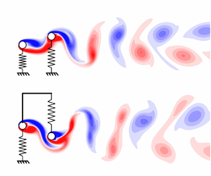
 $U_R \in [4,18]$. Three cases (figure 1) are considered to compare the elastically coupled and uncoupled tandem cylinder FIV. Case 1 represents the conventional elastically mounted uncoupled tandem cylinders. Case 2 and Case 3 represent the elastically coupled tandem cylinders, with the Strouhal frequency close to the natural frequency corresponding to the in-phase and out-of-phase vibration mode of the cylinders, respectively.
Problem definition and computational domain considered in the present work.

2. Computational model
An in-house fluid–structure interaction (FSI) solver is utilized to solve for elastically coupled multicylinder FIV. The solver is based on the sharp-interface immersed boundary method, as described by Mittal et al. (Reference Mittal, Dong, Bozkurttas, Najjar, Vargas and von Loebbecke2008) and Seo & Mittal (Reference Seo and Mittal2011). The solver was further extended to account for FIV of deformable structures (Bhardwaj & Mittal Reference Bhardwaj and Mittal2012) and elastically mounted cylinder (Garg, Soti & Bhardwaj Reference Garg, Soti and Bhardwaj2018). In the present study, the elastic coupling between two tandem cylinders placed in a cross-flow is prescribed. Two-dimensional simulations are carried out at a low Reynolds number,  $Re=100$. The flow past an isolated circular cylinder remains two-dimensional up to
 $Re < 188.5$ (Barkley & Henderson Reference Barkley and Henderson1996). However, the presence of a second cylinder in close proximity tandem configuration results in possible three-dimensional transition at a lower Reynolds number
 $Re \approx 110$ flow at
 $G = 3$ (Carmo, Meneghini & Sherwin Reference Carmo, Meneghini and Sherwin2010a,Reference Carmo, Meneghini and Sherwinb). Therefore, the flow across tandem cylinders at all the considered
 $G \in [1.1,5]$ can be assumed to be two-dimensional at
 $Re=100$. Furthermore, Leontini et al. (Reference Leontini, Thompson and Hourigan2006) reported the delay in the three-dimensional transition to a higher
 $Re$ flow due to the transverse motion of the cylinders. The following subsections describe the governing equations, problem set-up, and FIV quantification parameters used in the present study.
2.1. Governing equations
The fluid flow is governed by unsteady, incompressible and viscous Navier–Stokes equations, written in non-dimensional form as follows:
 $$\begin{gather} \boldsymbol{\nabla} \boldsymbol{\cdot} \boldsymbol{u} = 0, \end{gather}$$
 $$\begin{gather}\frac{\partial \boldsymbol{u}}{\partial t} + (\boldsymbol{u} \boldsymbol{\cdot} \boldsymbol{\nabla}) \boldsymbol{u} =-\boldsymbol{\nabla} p + \frac{1}{Re} {\nabla}^2 \boldsymbol{u}, \end{gather}$$
where dimensionless variables include flow velocity  $\boldsymbol {u}=\boldsymbol {u}^*/u^*_0$, pressure
 $p = p^* / \rho _f^* u_0^{* 2}$, time
 $t = u^*_0 t^* / D^*$ and Reynolds number (
 $Re = \rho _f^* u^*_0 D^* / \mu ^*$). The superscript
 $^*$ denotes a dimensional variable, and
 $u^*_0$,
 $\rho _f^*$,
 $D^*$ and
 $\mu ^*$ are free stream flow velocity, fluid density, cylinder diameter and dynamic viscosity, respectively. Definitions of major symbols are provided in table 1.
Definitions of the symbols used in the present study.

We consider the dynamics of two elastically mounted circular cylinders in a tandem arrangement, as shown in figure 1. This set-up is a simplified version of Price & Abdallah (Reference Price and Abdallah1990) for modelling FIV response of electrical conductor wires separated by elastic spacers. Here we consider cross-flow vibrations of cylinders with 1-DOF with equal mass ratio  $m$ and zero damping. The equation of motion of an elastically coupled cylinder system is as follows:
 \begin{equation} \begin{bmatrix} 1 & 0 \\ 0 & 1 \end{bmatrix} \begin{bmatrix} \ddot{y}_1 \\ \ddot{y}_2 \end{bmatrix} + \begin{bmatrix} k_{1}+k_{2} & -k_{2} \\ -k_{2} & k_{2}+k_{3} \end{bmatrix} \begin{bmatrix} y_1 \\ y_2 \end{bmatrix} = \begin{bmatrix} 4 F_{T 1}/{\rm \pi} m \\ 4 F_{T 2}/{\rm \pi} m \end{bmatrix}, \end{equation}
where  $y_i=y_i^*/D^*$ is the non-dimensional transverse amplitude of displacement and
 $F_{T i} = F_{T i}^*/\rho _f^* u_0^{* 2} D^*L^*$ is the non-dimensional transverse force on the
 $i$th cylinder. Here we have
 $i=1$ for the UC and
 $2$ for the DC. Here
 $k_{i}=k_i^* D^{* 2}/m_{s}^* u_0^{* 2}$ is the non-dimensional reduced stiffness, and
 ${4 m_s^*}/{{\rm \pi} \rho _f^* D^{* 2}}L^*$ is the mass ratio (
 $m_1=m_2=m$) of the cylinders. Here
 $y_i$,
 $\dot {y}_i$ and
 $\ddot {y}_i$ represent the instantaneous displacement, velocity and acceleration of the
 $i$th cylinder. Here
 $L^*$ is the cylinder spanwise length and is taken as unity in the present study.
For the conventional tandem cylinder configuration (Case 1), the reduced stiffness values are  $k_1=k_3$ and
 $k_2=0$. Substituting these values in (2.4a,b)–(2.5a,b) gives
 $f_{n1}=f_{n2}=\sqrt {k_1}/2 {\rm \pi}$, with
 $\sigma _1=1$ and
 $\sigma _2=-1$. This implies that the uncoupled tandem cylinder system has a single natural frequency, with any linear combination of the two mode shapes (
 $[1,1]^{\rm T}$ and
 $[-1,1]^{\rm T}$) as the associated mode shape. This is why there is no specific mode shape or
 $\phi _{y12}$ associated with uncoupled tandem cylinders. However, for Cases 2 and 3, elastic coupling is introduced via an additional spring with stiffness
 $k_2 \neq 0$. Owing to the coupling stiffness
 $k_2$, the system bifurcates into two natural frequencies (
 $\,f_{n1}$ and
 $\,f_{n2}$) and associated modal amplitude ratios (
 $A_{n1}/A_{n2}=\sigma _{n1}$ and
 $\sigma _{n2}$, respectively):
 $$\begin{gather} f_{n 1} = \cfrac{1}{2 {\rm \pi}} \sqrt{ \cfrac{k_1+k_3}{2} + k_2 - \sqrt{ \left( \cfrac{k_1-k_3}{2} \right)^2 + k_2^2}} ,\quad \sigma_{n 1} = \sqrt{1 + \left( \cfrac{k_1-k_3}{2 k_2} \right)^2} - \cfrac{k_1-k_3}{2 k_2}, \end{gather}$$
 $$\begin{gather}f_{n 2} = \cfrac{1}{2 {\rm \pi}} \sqrt{\cfrac{k_1+k_3}{2} + k_2 + \sqrt{ \left( \cfrac{k_1-k_3}{2} \right)^2 + k_2^2}} ,\quad \sigma_{n 2} =-\sqrt{1 + \left( \cfrac{k_1-k_3}{2 k_2} \right)^2} - \cfrac{k_1-k_3}{2 k_2}. \end{gather}$$
2.2. Simulation set-up
The FIV of two circular cylinders in the tandem configuration is studied in an open domain flow of  $Re=100$ as shown in figure 1. The open domain is simulated by enforcing constant inflow velocity on the upstream wall (
 $u=1,v=0$). The free slip boundary condition (
 $\partial u/\partial y=0,v=0$) is imposed on the side walls of the considered domain. The right-hand boundary is prescribed with a fully developed boundary condition (
 $\partial u/\partial x=0,\partial v/ \partial x=0$). Two tandem cylinders, with gap ratio
 $G$ varying systematically from
 $1.1$ to
 $5$, are immersed in the flow. The fluid–structure interface is imposed with no-slip boundary condition (
 $(\boldsymbol {\nabla } \boldsymbol {u})\boldsymbol{\cdot}\boldsymbol {\hat {n}} = 0$). The cylinders are constricted to move only in the transverse direction. The mass ratio of both cylinders is kept constant at
 $m=10$, with no damping
 $\xi =0$.
The reduced stiffness values  $k_1,k_2,k_3$ are varied systematically to obtain multiple structural vibration configurations. The excitation force frequency is primarily assumed to be
 $\approx St_{00} \sim St_0$. Therefore, only the natural frequency closer to
 $St_0$ is assumed to be excited in a particular case. The stiffness parameters proposed by Ding et al. (Reference Ding, Srinil, Bao, Zhou and Han2020) are used in the present analysis to excite individual modes (see the Appendix) during FIV of tandem cylinders. First,
 $k_1=k_3\in [0.12,2.47];k_2=0$, corresponding to
 $U_R = u_0^*/f_{n}^* D^* \in [4,18]$, is used in Case 1. In Case 2,
 $k_1=6,k_2\in [0.12,8.19];k_3=0$ configuration is used to ensure
 $f_{n2} \gg St$ for
 $U_{R}=u_0^*/f_{n1}^* D^* \in [4,18]$. Finally, the Case 3 configuration is realized using
 $k_1=0.1,k_2\in [0.018,8.19];k_3=0$ such that
 $f_{n1} \ll St_0$ for
 $U_{R}=u_0^*/f_{n2}^* D^* \in [4,18]$.
The computational method used in the present study, is briefly described in § S1 of the supplementary material available at https://doi.org/10.1017/jfm.2023.910. Based on the domain and grid independence tests (see § S2 in the supplementary material), a Cartesian grid of  $1024 \times 256$ distributed over a domain size of
 $85 \times 30$, with grid size
 $\Delta x = \Delta y = 0.02$ in the refined regions, is utilized to perform all the subsequent simulations at time step size
 $\Delta t = 0.01$. Further, the solver is verified (see § S3 in the supplementary material) and shows good agreement with Ding et al. (Reference Ding, Srinil, Bao, Zhou and Han2020) for elastically coupled FIV of side-by-side cylinders.
2.3. The FIV quantification parameters
Several quantification variables are used to compare and contrast the FIV response across different cases,  $G$ and
 $U_R$. The cylinder displacements
 $A_i$ correspond to the maximum FIV displacement amplitude, with bars indicating the localized cycle-to-cycle amplitude fluctuations. The maximum coefficient of fluctuating transverse force on the two cylinders is given by
 \begin{equation} C_{Ti}^\prime =2 F_{Ti}^\prime = 2 (F_{Ti} - \bar{F}_{Ti})_{max}. \end{equation}
The transverse force is composed of potential ( $C_{Pi}=-2 C_{a} ({\rm \pi} /4) \ddot {y}_i$) and vortex (
 $C_{vi} = C_{Ti}-C_{Pi}$) force components (Lighthill Reference Lighthill1986; Govardhan & Williamson Reference Govardhan and Williamson2000). Here
 $C_{a}$ is the added mass coefficient and is assumed to be
 ${\approx }1$, corresponding to the isolated cylinder case (Govardhan & Williamson Reference Govardhan and Williamson2000). Further, the stationary
 $i$th cylinder mean drag
 $\bar {C}_{Di}$ and maximum fluctuating lift
 $C_{Li}^\prime$ is also presented for varying
 $G$.
To remove spurious oscillations in signals of displacement and fluid force, we utilized a Butterworth filter with a non-dimensional cutoff frequency of unity. Typically,  $50$ vibration cycles after reaching dynamically steady state were considered for the analysis. The simulations are executed for at least
 $t = 1200$ and longer, if required, to ensure a dynamic steady state. Some sample signals with delayed dynamic steady state are shown in § S5. The amplitude spectral density (ASD) of displacement (
 $y_i$) and transverse force (
 $C_{Ti}$) is normalized using the corresponding structural natural frequency
 $f = f_{signal}/f_{ni}$ (
 $i=1$,
 $1$ and
 $2$ for Cases 1, 2 and 3, respectively). The ASD of the signals at each
 $U_R$ is interpolated using histogram distribution on a common frequency scale of
 $0$ to
 $4$ with
 $\Delta f=0.025$ and normalized with the maximum strength of the frequency signal at that
 $U_R$, and plotted on a logarithmic scale. The colourmap is superimposed with the normalized Strouhal frequency
 $f_{St_{00}}=St_{00}/f_{ni}$ using a dotted blue line.
Here  $\phi _{C_{Ti}}$ and
 $\phi _{C_{vi}}$ denote phase difference of
 $C_{Ti}$ and
 $C_{vi}$ with
 $y_i$, respectively. Furthermore,
 $\phi$ is obtained using the phase difference between the ASD frequency component of the two signals, corresponding to the dominant
 $y_i$ frequency at that
 $U_R$. Further, the intercylinder phase difference
 $\phi _{y12}$,
 $\phi _{C_{T12}}$ and
 $\phi _{C_{L12}}$ indicate the phase lag of
 $y_2$,
 $C_{T2}$ and
 $C_{L2}$ from
 $y_1$,
 $C_{T1}$ and
 $C_{L1}$, respectively, corresponding to the dominant frequency of
 $y_1$,
 $C_{T1}$ and
 $C_{L1}$. All the phase differences are indicated in degrees.
The angular locations  $\theta _i$ are measured from the front stagnation point location of the
 $i$th cylinder in stationary isolated configuration. The vortex formation length
 $L_{u^\prime u^\prime }$ is quantified as the downstream distance of the vortex formation point from the centre of the cylinder. The vortex formation point is defined as the location in the flow where the fluctuating component of the axial velocity becomes maximum (Green & Gerrard Reference Green and Gerrard1993). The localized mean coefficient of pressure
 $C_{Pi}=p^*_i/(1/2 \rho _f^* u_0^{* 2})$ and coefficient of skin friction
 $C_{Fi}=\tau _i^*/(1/2 \rho _f^* u_0^{* 2})$ is plotted using solid lines, with shaded regions indicating the transient variations in
 $C_{Pi}$ and
 $C_{Fi}$ at the corresponding
 $\theta _i$ locations. The separation (reattachment)
 $\theta _i$ correspond to a positive to negative (negative to positive) transition of
 $C_{Fi}$ on the cylinder surface. The localized gap flow velocity
 $c_g$ is quantified as the flow velocity normal to the line joining the centres of the UC and DC. The transient gap flow
 $F_g$ is obtained as the total volume flow rate across the line joining UC and the DC. Further, energy transfer from the fluid to the cylinder is quantified as the rate of work done by the flow on the cylinder,
 $W_i = C_{Ti} \dot {y}_i$.
The dynamic mode decomposition (DMD) is performed on the vorticity field for quasiperiodic FIV responses. We use the methodology and the algorithm described by Schmid (Reference Schmid2010), Sayadi et al. (Reference Sayadi, Schmid, Nichols and Moin2013) and Kutz et al. (Reference Kutz, Brunton, Brunton and Proctor2016). All the field data, corresponding to the mesh columns of the oscillating cylinders, is neglected during DMD analysis and later plotted after linear interpolation for those regions. Here  $|\alpha _i|$ shows the strength of corresponding modal frequencies. A typical case consists of at least 500 snapshots for periodic and up to 1800 snapshots for quasiperiodic FIV response at non-dimensional time interval of 0.1. Further details of the methodology have been discussed in Sharma et al. (Reference Sharma, Pandey and Bhardwaj2022b).
3. Characteristics of cylinder vibrations
In this section, we report the FIV amplitudes of the tandem upstream ( $A_1$) and downstream (
 $A_2$) cylinder for Cases 1, 2 and 3, for
 $G \in [1.1,5]$ and
 $U_R \in [4,18]$.
3.1. Case 1: elastically uncoupled cylinders
The UC FIV response (figure 2a) for  $2 \leq G \leq 5$ is quite similar to the VIV response of an isolated circular cylinder (Prasanth & Mittal Reference Prasanth and Mittal2009). Here
 $A_1$ shows an initial jump to
 ${\sim }0.65$ and is gradually reduced to
 ${\sim }0.2$ during lock-in, with amplitude variations similar to upper and lower branch variations at high
 $Re$ (Govardhan & Williamson Reference Govardhan and Williamson2000). The initial and final desynchronization have negligible
 $A_1$ (
 ${\sim }O(10^{-3})$ and
 ${<}0.05$, respectively). Although some variations in
 $U_R$ correspond to various jumps in
 $A_1$, the qualitative features remain consistent for various
 $G$. While the DC FIV response
 $A_2$ (figure 2b) exhibits some similarities with the UC, the following are some important differences. The
 $A_2$ for
 $G \geq 2$ shows an initial jump, similar to
 $A_1$. However,
 $A_2$ is lower (
 ${\sim }0.4$) than
 $A_1$ (
 ${\sim }0.65$), and continuously increases with
 $U_R$. Furthermore,
 $A_2$ shows a sharp jump to
 ${\sim }1.0$ at
 $U_R \sim 7$ for all
 $G \geq 2$, and further gradually decreases with increasing
 $U_R$. The
 $A_2$ is much larger (nearly double) than
 $A_1$ in this regime. Finally,
 $A_2$ drops to very small amplitudes at large
 $U_R$, corresponding to the final desynchronization of the UC. However,
 $A_2$ remains
 $> 0.1$ in the desynchronization regime for
 $G > 2$, even at very large
 $U_R$. The larger
 $A_2$ is possibly due to the interactions of the UC wake with the DC, resulting in WIV (Assi et al. Reference Assi, Bearman and Meneghini2010, Reference Assi, Bearman, Carmo, Meneghini, Sherwin and Willden2013).
Variation of amplitude with reduced velocity ( $U_R$) for (a,c,e) upstream cylinder,
 $A_1$, and (b,d,f) downstream cylinder,
 $A_2$: (a,b) Case 1, elastically uncoupled; (c,d) Case 2, elastically coupled, Mode 1; (e,f) Case 3, elastically coupled, Mode 2. Difference cases of gap ratio
 $G$ are compared in each panel. The insets in (a,c,e) represent the configuration for Case 1, 2 and 3, respectively.

The FIV response for uncoupled tandem cylinders (Case 1) with  $2 \leq G \leq 5$ is broadly classified into four regimes. The first regime is initial desynchronization (ID) at very low
 $U_R$. The second regime corresponds to the amplitude jumps for both cylinders with
 $A_1>A_2$. The third regime is initiated by a secondary jump in
 $A_2$, resulting in
 $A_2>A_1$. Finally, the fourth regime is the final desynchronization of
 $A_1$ and
 $A_2 \sim 0.1$, corresponding to WIV. The observed characteristics are consistent with previous numerical (Papaioannou et al. Reference Papaioannou, Yue, Triantafyllou and Karniadakis2008; Borazjani & Sotiropoulos Reference Borazjani and Sotiropoulos2009; Prasanth & Mittal Reference Prasanth and Mittal2009; Bao et al. Reference Bao, Huang, Zhou, Tu and Han2012; Griffith et al. Reference Griffith, Jacono, Sheridan and Leontini2017) and experimental (King & Johns Reference King and Johns1976; Ruscheweyh Reference Ruscheweyh1983; Allen & Henning Reference Allen and Henning2003; Narvaez, Schettini & Silvestrini Reference Narvaez, Schettini and Silvestrini2020; Xu et al. Reference Xu, Wu, Jia and Wang2021) studies. Notably, the transition between the second and third regime occurs at
 $U_R \sim 7$ for all
 $G \geq 2$, corresponding to
 $f_n \sim 0.14$. This is close to
 $St_{00}$ in the presence of gap vortices (figure S4c) and is consistent with the finding of Prasanth & Mittal (Reference Prasanth and Mittal2009) that the transition occurs when
 $St_{00} \sim f_n$. It is worth highlighting that Gu et al. (Reference Gu, Xu, Jiang and Yao2023) also studied the effect of
 $G \in [2,6]$ on 2-DOF vibrations of tandem square cylinders at
 $Re=100$ and observed qualitatively similar
 $A_1$ and
 $A_2$ variation. In their study, the peaks of
 $A_1 \sim 0.65$ and
 $A_2 \in [0.85,1]$ are also close to the peaks
 $A_1 \sim 0.65$ and
 $A_2 \sim 1.0$ of the present study, even though the cross-sections are significantly different. However, Qin et al. (Reference Qin, Alam and Zhou2019) performed experimental investigations on tandem circular cylinders for systematic variation in
 $G \in [1.2,6]$ at
 $Re \sim O(10^4)$. They observed significant changes in
 $A_1$ and
 $A_2$ with variation in
 $G$, which are not reflected in the present study. This is possibly caused due to galloping vibrations occurring at high
 $Re$, resulting in high FIV amplitudes at high
 $U_R$. Moreover, they study the damped vibrations (
 $m \zeta \sim 0.58$), contrary to the present undamped vibration study (
 $m \zeta = 0$), resulting in very small VIV contributions in their study.
The  $G = 1.1$ results significantly differ from the cylinders with larger
 $G$. The cylinders show an initial jump in
 $A_1$ and
 $A_2$ at
 $U_R = 5.25$. Eventually, both cylinders show continuously increasing FIV amplitudes, with
 $A_1$ and
 $A_2$ reaching
 ${\sim }1.0$ and
 ${\sim }1.1$ at
 $U_R = 18$, respectively. A minor jump in both amplitudes is observed at
 $U_R = 9$. Chung (Reference Chung2017) (
 $Re = 100$) reported a similar galloping response for independent elastically mounted tandem cylinders corresponding to
 $G \leq 1.7$. However, some of their characteristics differ from the present study. In Chung (Reference Chung2017),
 $A_1$ is slightly higher than the present study, and
 $A_2$ shows a drop at
 $Ur=10$, which is not observed in the present study. This is likely due to their lower mass ratio (
 $m=2$) than the present study (
 $m=10$) and an additional vibration mode of the cylinders in the in-line direction. Similarly, Chen et al. (Reference Chen, Ji, Williams, Xu, Yang and Cui2018) (
 $Re=100$) observed a galloping response for three tandem cylinders, with diverging amplitudes at
 $G = 1.2$ and almost constant amplitudes at
 $G = 1.5$. Kim et al. (Reference Kim, Alam, Sakamoto and Zhou2009) (
 $Re=O(10^5)$) also reported a similar galloping response for tandem cylinder FIV at
 $G = 1.1$ and
 $1.3$, at large
 $m \zeta$. Interestingly, Qin et al. (Reference Qin, Alam and Zhou2019) observed a continuous galloping response for
 $G \leq 1.5$ and a delayed galloping response for
 $G \leq 3$, for high
 $m \zeta$ tandem cylinders at high
 $Re \sim O(10^4)$.
3.2. Case 2: elastically coupled cylinders Mode 1
As shown in § 2.1, only Mode 1 (see inset in figure 2c) is excited for Case 2, i.e. the cylinders are bound to vibrate in-phase ( $\phi _{y12} = 0$). Figure 2(c) shows a significantly weaker FIV response for the UC, as compared with Case 1. The maximum
 $A_1 \sim 0.2$ is substantially lower than
 $A_1 \sim 0.65$, corresponding to Case 1. Here
 $A_1$ shows an initial jump similar to the initial branch. It is followed by a gradually decreasing
 $A_1$ similar to lock-in. The drop in
 $A_1$ at desynchronization is also gradual and not sharp compared with Case 1.
In figure 2(d), the DC attains  $A_2 \sim 0.9$ for
 $G>2$, and slightly lower values for
 $G = 1.1$ (
 $A_2 \sim 0.4$) and
 $G = 2$ (
 $A_2 \sim 0.6$). The jump in the initial branch for
 $A_2$ occurs at almost the same
 $U_R$, corresponding to the transition from regime 1 to 2 in Case 1. The only exception is
 $G = 2$, for which the jump corresponds to the
 $U_R$ of the second amplitude jump between regimes 2 and 3 in Case 1. For Case 2,
 $A_2$ (
 $G>2$) attains a higher magnitude than their Case 1 counterpart (regime 2). However, the
 $A_2$ curve, corresponding to the second amplitude jump (
 $G = 2$), attains a lower magnitude than its Case 1 counterpart (regime 3). The inconsistent behaviour of
 $G = 2$ is likely due to the unfavourable time delay of vortices between the two cylinders. The
 $\phi _{C_{L12}}\sim 90^{\circ }$ indicates a slight delay from the desired modal in-phase forcing of Case 2. As the cylinders vibrate, the vortex path between the cylinders elongates, resulting in a more antiphase nature of the fluid forces. This phenomenon is similar to ‘modal decoupling’, reported by Price & Abdallah (Reference Price and Abdallah1990), that leads to FIV suppression even if the excitation frequency is closer to the cylinder's natural frequency. In this context, previous studies on rigidly coupled two tandem cylinders have realized
 $\phi _{y12}=0$, similar to Case 2. For example, Zhao (Reference Zhao2013) studied the rigidly coupled tandem cylinders at
 $Re=150$ and observed a similar VIV-type amplitude variation curve. Similar to the present study, the FIV amplitudes in their study (
 $A_1=A_2$) were smaller for
 $G = 1.5$ (
 $A_1 \sim 0.2$) and
 $2$ (
 $A_1 \sim 0.6$), as compared with
 $G \geq 4$ (
 $A_1 \sim 0.9$). Zhao, Murphy & Kwok (Reference Zhao, Murphy and Kwok2016) also reported a VIV-type response variation in
 $A_1=A_2$ for rigidly coupled tandem cylinders at
 $Re=5000$ for
 $G>1.5$.
While rigid coupling enforces  $A_1=A_2$, even if the two cylinders experience different flow forces, we report significant amplitude variations between
 $A_1$ and
 $A_2$ for the elastic coupling. This shows the implications of flow force and mode shape interactions between the two cylinders. The
 $A_1/A_2$ (
 ${\sim }1/3$) variation is introduced in the side-by-side configuration of Ding et al. (Reference Ding, Srinil, Bao, Zhou and Han2020) for the same mode shape. However,
 $A_1/A_2$ in the present study is
 ${\sim }0.2$ for tandem configuration with the same structural parameters. Therefore, enhanced transverse forces on the DC modify the relative FIV amplitudes in the present case. A detailed description of flow forces on the cylinders is discussed in § S7.
While  $G = 1.1$ (Case 1) shows a galloping-like response (§ 3.1),
 $G = 1.1$ (Case 2) shows a VIV-like response. Zhao (Reference Zhao2013) also observed this behaviour at
 $Re=150$ and
 $G = 1.5$, reporting an exceptionally low FIV amplitude. Galloping is possibly due to
 $\phi _{y12} \neq 0$ induced between the tandem cylinders in Case 1. The modal arrangement enforces
 $\phi _{y12} = 0$ in Case 2, possibly suppressing galloping at small
 $G$. Maeda et al. (Reference Maeda, Kubo, Kato and Fukushima1997) also observed the absence of galloping for rigidly connected tandem cylinders (
 $m \zeta \sim 0.46$) at
 $Re \sim O(10^4)$, with a resumption of galloping in a slightly staggered arrangement. However, Zhao et al. (Reference Zhao, Murphy and Kwok2016) observed a galloping-like response for the rigidly connected tandem cylinders (
 $m = 2.5, \zeta = 0$) at
 $G = 1.5$ in an
 $Re=5000$ flow. Similar behaviour is also reflected in the FIV response of elliptical cylinders (single body approximation for closely placed tandem cylinders), as a narrow lock-in at low
 $Re$ (Yogeswaran et al. Reference Yogeswaran, Sen and Mittal2014) and an elongated lock-in at high
 $Re$ (Zhao, Hourigan & Thompson Reference Zhao, Hourigan and Thompson2019). Therefore,
 $\phi _{y12}=0$ configuration tandem cylinders at very small
 $G$ can exhibit galloping response at sufficiently smaller
 $m$ and larger
 $Re$.
3.3. Case 3: elastically coupled cylinders Mode 2
Similar to Case 2, only Mode 2 (see inset in figure 2e) is excited for Case 3, i.e. the cylinders are bound to move out-of-phase ( $\phi _{y12} = 180^{\circ }$). The UC with
 $G \geq 2$ attains
 $A_1 \sim 0.9$ during the lock-in, which is larger than the Case 1 or 2 counterparts. Similarly, the DC attains
 $A_2 \sim 0.75$ for
 $G>2$ in the lock-in regime. Similar to Case 2, both
 $A_1$ and
 $A_2$ do not show any amplitude jump in the middle of the lock-in branch, contrary to Case 1. The initiation of the lock-in is reflected by a sharp jump in
 $A_1$ and
 $A_2$ for
 $G = 2$, which is synchronized with the first amplitude jump in Case 1. The jump in
 $A_1$ and
 $A_2$ during the lock-in initiation becomes increasingly gradual for
 $2 \leq G \leq 5$. Interestingly, the reduction gradient of
 $A_1$ and
 $A_2$ towards the end of lock-in becomes steeper for
 $2 \leq G \leq 5$.
Like Cases 1 and 2, the DC exhibits WIV ( $A_2 \sim 0.1$) in the high
 $U_R$ desynchronized regime for
 $G \geq 3$ in Case 3. Surprisingly, for this Case, the lock-in regime for
 $G = 2$ extends up to
 $U_R = 13$, beyond its Case 2 counterpart. This is slightly beyond
 $U_R = 11.5$, corresponding to the desynchronization of
 $G = 2$ tandem cylinders in Case 1. Furthermore, an initial local maxima of
 $A_1 \sim A_2 \sim 0.5$ is attained in the low
 $U_R$ regime for
 $G \geq 4$, with significant amplitude fluctuations (§ 4.3). This is similar to the initial branch behaviour in VIV. However, instead of growing monotonically,
 $A_1$ and
 $A_2$ reach a local maxima and decrease until lock-in begins.
Furthermore,  $\phi _{y_{12}}= 180^{\circ }$ has been reported for connected tandem cylinders. Examples include controlling relative motion using complex thread linkages (Brika & Laneville Reference Brika and Laneville1997; Laneville & Brika Reference Laneville and Brika1999) or pivoting the rigidly coupled cylinders at the centre (Arionfard & Nishi Reference Arionfard and Nishi2018b,Reference Arionfard and Nishia). Laneville & Brika (Reference Laneville and Brika1999) observed multiple peaks for the FIV of cylinders at
 $Re \sim O(10^4)$ and
 $G>10$, with significant hysteresis in the low
 $U_R$ peaks. Similarly, Arionfard & Nishi (Reference Arionfard and Nishi2018b) observed two vibrations amplitude peaks at
 $U_R = 5.5$ and
 $7.3$ for
 $G = 3.9$ at
 $Re \sim O(10^3)$. While these studies are not exactly similar to the present case, they provide a reasonable correlation with the observations of Case 3.
Interestingly, the  $G = 1.1$ in Case 3 shows a galloping response similar to Case 1. The amplitude jumps in
 $A_1$ and
 $A_2$ occur at the same
 $U_R$ compared with the Case 1 counterpart. While the FIV amplitudes in Case 3 are lower than in Case 1, the relative amplitudes between the two cylinders (
 $A_1/A_2 \sim 0.7$) are very similar. The kinks in
 $A_i$ observed at
 $U_R \geq 13$ correspond to the amplitude fluctuations (§ 4.4).
4. Characteristics of the FIV regimes
The variations in  $A_1$ and
 $A_2$ give a basic prediction of different regimes of FIV distributed over
 $U_R \in [4, 18]$ and
 $G \in [1.1, 5]$ across different cases. However, other parameters like force, spectral and intracylinder and intercylinder phase characteristics must be observed collectively for final regime classification. The overall FIV response has been classified broadly into 10 regimes (figure 3): ID; IDG; IB; MM; UB; LB; LN; FD; WIV; GD. Additionally, stationary tandem cylinder regimes are classified as those without gap vortices (ST) and those with gap vortices (STG). We do not segregate UB and LB regimes of lock-in of Cases 2 and 3, and will be explained in the following subsections.
Classification of FIV regimes in the  $U_R$–
 $G$ plane for (a) Case 1, (b) Case 2 and (c) Case 3. The regimes are as follows: initial desynchronization (ID); initial desynchronization with gap vortices (IDG); initial branch (IB); mixed mode (MM); upper branch lock-in (UB); lower branch lock-in (LB); lock-in (LN); final desynchronization (FD); wake-induced vibration (WIV); and galloping domination (GD). The regimes for stationary tandem cylinders are shown at
 $U_R = 0$ and are classified as without (ST) and with (STG) gap vortices.

The overall flow force characteristics (discussed in § S7) show sharp contrast across Cases 1, 2 and 3. Therefore, for a better understanding of the branching characteristics and brevity of the study, each case is discussed using individual representative  $G$. In this section, we report the characterization of different FIV regimes across Cases 1, 2 and 3, including galloping. The FIV amplitudes, flow forces, ASD and phase characteristics are collectively analysed to classify and understand the FIV regimes. The classification of the regimes is based on the criteria described earlier by Sharma et al. (Reference Sharma, Garg and Bhardwaj2022a, table 2).
4.1. The FIV regimes of Case 1
As observed in § 3, the overall FIV response in Case 1 ( $G > 1.1$) is classified broadly into the following regimes: IDG and ID; UB and LB lock-in; FD or WIV. Since FIV responses for the gap ratios (
 $G > 1.1$) of Case 1 are qualitatively similar, we discuss a representative case of
 $G = 4$. Figures 4(a) and 4(b) show that
 $A_1$ and
 $A_2$ are negligible (
 ${<}0.01$) in the ID regime (
 $U_R \in [4,5.25]$). The
 $C_{T1}^\prime$ and
 $C_{V1}^\prime$ remain negligible (
 ${\sim }0.01$) with increasing
 $U_R$ in this regime, with
 $C_{T2}^\prime$ and
 $C_{V2}^\prime$ having finite decreasing magnitude. Interestingly, these flow forces are significantly lower than the stationary cylinder counterpart (
 $C_{L_0}^\prime \sim 0.403$) at
 $G = 4$, indicating stronger FIV suppression characteristics with increasing
 $U_R$. The
 $f_{y1}$,
 $f_{y2}$,
 $f_{C_{T1}}$ and
 $f_{C_{T2}}$ indicate single dominant frequency component parallel to
 $f_{St_{00}}$, with a slightly lower frequency. The lower frequency results from the absence of gap vortices in this regime (shown in § 6), contrary to the stationary cylinder flow with gap vortices. Finally,
 $\phi _{C_{Ti}}$ and
 $\phi _{C_{Vi}}$ remain
 ${\sim }0^{\circ }$ in this regime. Therefore, this regime is identified as the ID regime.
The FIV characterization for Case 1 at  $G = 4$: (a,b) shows
 $A_1$ and
 $A_2$, with bars representing cycle-to-cycle amplitude variation. Variation of
 $C_{Ti}^\prime$ (dotted blue),
 $C_{Vi}^\prime$ (dotted red) and
 $C_{Li}^\prime$ (dotted black) are plotted for the (c) upstream (
 $i=1$, a,c,e,g,i) and (d) downstream (
 $i=2$, b,d,f,h,j) cylinders. Contours show
 $f_{yi}$ (e,f) and
 $f_{C_{Ti}}$ (g,h) with the dotted blue line representing
 $f_{St_{00}}$ for
 $G = 4$. Here
 $\phi _{C_{Vi}}$ (dotted red) and
 $\phi _{C_{Ti}}$ (dotted blue) are plotted for (i) upstream and (j) downstream cylinders.

The second regime ( $U_R \in [5.5,6.75]$) shows sharp jumps in
 $A_1$ and
 $A_2$ during the transition from ID regime to this regime, indicating a narrow IB regime near
 $U_R =5.5$. The amplitudes
 $A_1 \sim 0.6$ (nearly constant) and
 $A_2 \sim 0.4$ (gradually increasing) remain high throughout this regime, with
 $A_1>A_2$. After a sudden jump in flow forces, both the cylinders show a decreasing
 $C_{Ti}^\prime$ and an increasing
 $C_{Vi}^\prime$. Dominant frequency components of
 $f_{yi}$ and
 $f_{C_{Ti}}$ are observed at
 ${\sim }1$ in this regime, with additional third harmonic signatures in
 $f_{C_{Ti}}$. Furthermore,
 $\phi _{C_{Vi}}$ jumps from
 $0^{\circ }$ to
 $180^{\circ }$ at the start of this regime, with
 $\phi _{C_{Ti}} \sim 0^{\circ }$ throughout this regime. Therefore, this regime is identified as the UB regime.
The  $A_1$ starts gradually decreasing in the third regime (
 $U_R \in [7,8.75)$). The
 $A_2$ jumps to
 ${\sim }1.0$ during the transition and remains nearly constant in this regime. After reaching a local maxima,
 $C_{V1}^\prime$ gradually reduces, with much smaller
 $C_{T1}^\prime$. The
 $C_{V2}^\prime$ also shows a gradual reduction in this regime after a sharp jump during the transition from the UB regime. The
 $f_{yi}$ and
 $f_{C_{Ti}}$ show dominant components at
 ${\sim }1$, with third harmonic signatures in
 $f_{C_{Ti}}$. Additionally,
 $\phi _{C_{Ti}}$ transitions from
 $0^{\circ }$ to
 $180^{\circ }$ in this regime, with
 $\phi _{C_{Vi}} \sim 180^{\circ }$. Therefore, this regime is identified as the LB lock-in regime. While in Case 1,
 $A_2$ is significantly larger in LB than UB, we choose to designate it as LB for continuity.
The initiation of the fourth regime ( $U_R > 8.75$) is characterized by a sudden initial drop in
 $A_1$ (
 ${<}0.07$) and
 $A_2$ (
 ${<}0.27$), followed by a gradual reduction with increasing
 $U_R$. The
 $C_{T1}^\prime$ and
 $C_{T2}^\prime$ asymptotically approach
 $C_{L1}^\prime$ and
 $C_{L2}^\prime$, respectively. The
 $f_{yi}$ and
 $f_{C_{Ti}}$ shows single frequency components coinciding to
 $f_{St_{00}}$, with
 $\phi _{C_{Ti}}$ and
 $\phi _{C_{Vi}}$ at
 $180^{\circ }$. The spectral characteristics show desynchronization, with
 $A_2 > A_1$ and
 $C_{T2}^\prime \gg C_{T1}^\prime$. This indicates that the DC experiences an additional FIV excitation due to the wake of the UC. Therefore, this regime is identified as the WIV regime, continuing with the nomenclature proposed by Assi et al. (Reference Assi, Bearman, Carmo, Meneghini, Sherwin and Willden2013).
4.2. The FIV regimes of Case 2
The ID regime of Case 2 is characterized by negligible  $A_1$ and
 $A_2$ (
 $< 0.01$) for
 $U_R \in [4,5.5]$. The
 $C_{T1}^\prime$,
 $C_{V1}^\prime$ are of
 $O (10^{-3})$, and
 $C_{T2}^\prime$,
 $C_{V2}^\prime$ of
 $O(10^{-1})$; with decreasing magnitude for increasing
 $U_R$. Dominant components of
 $f_{yi}$ and
 $f_{C_{Ti}}$ are parallel to
 $f_{St_{00}}$ with slightly lower frequency due to the absence of gap vortices. Similar to Case 1, Case 2 exhibits FIV suppression characteristics in this regime. Interestingly,
 $\phi _{C_{T1}} \approx \phi _{C_{V1}} \sim 80^{\circ }$ and
 $\phi _{C_{T2}} \approx \phi _{C_{V2}} \sim 360^{\circ }$ shows a deviation from the expected
 $0^{\circ }$ phase difference response in this regime.
The  $U_R \in [5.5, 6.0]$ shows a gradual increase in
 $A_i$, accompanied by sharp increase in
 $C_{Ti}^\prime$ and
 $C_{Vi}^\prime$. The
 $A_i$ show minor cycle-to-cycle fluctuations (indicated by bars in figure 5a,b), which are reflected in the ASD characteristics
 $f_{yi}$ and
 $f_{C_{Ti}}$. Therefore, this regime corresponds to the IB.
The FIV characterization for Case 2 at  $G = 4$. The rest of the caption is the same as in figure 4.

Similar to the isolated cylinder lock-in branch,  $U_R \in [6.0,7.75]$ shows steady and high values of
 $A_1$ (
 ${\leq }0.2$) and
 $A_2$ (
 ${\leq }1.0$). The ASD characteristics show dominant
 $f_{yi}$ and
 $f_{C_{Ti}}$ close to
 $1$, with third harmonic signatures in
 $f_{C_{Ti}}$. However, the ASD signatures show a minor gradient in associated frequencies with
 $U_R$. Further, the magnitude (
 $C_{Ti}^\prime$ and
 $C_{vi}^\prime$) and phase (
 $\phi _{C_{Ti}}$ and
 $\phi _{C_{vi}}$) of flow forces do not exhibit any explicit UB- or LB-like behaviour. For example, the decreasing
 $C_{T1}^\prime$ and
 $C_{V1}^\prime$ indicate a lower branch behaviour, however,
 $C_{T2}^\prime$ and
 $C_{V2}^\prime$ variations do not confirm to that behaviour. Furthermore,
 $\phi _{C_{T}}$ and
 $\phi _{C_{v}}$ of a freely oscillating cylinder (e.g. isolated cylinder or Case 1 configuration) vary between
 $0^{\circ }$ and
 $180^{\circ }$. The phase of forces in Cases 2 and 3 may vary anywhere between
 $0^{\circ }$ and
 $360^{\circ }$ due to the presence of elastic coupling between the cylinders. In this context, Zhao (Reference Zhao2013) also observed multiple phase jumps for the rigidly coupled cylinders. Therefore, the conventional classification of branches via flow force magnitude and phase is invalid for Cases 2 and 3. We refer to this regime as LN.
The  $U_R > 8$ regime of Case 2 shows a WIV response, similar to Case 1. Here
 $A_1 < 0.01$ and
 $A_2 \sim 0.13$ are observed at high
 $U_R$, with
 $C_{T1}^\prime$ and
 $C_{T2}^\prime$ asymptotically approaching
 $C_{L1}^\prime$ and
 $C_{L2}^\prime$, respectively. The
 $f_{yi}$ and
 $f_{C_{Ti}}$ show dominant frequencies along
 $f_{St_{00}}$, indicating a WIV regime. The
 $\phi _{C_{T2}} \approx \phi _{C_{V2}}$ remain
 $180^{\circ }$ for the whole regime. However,
 $\phi _{C_{T1}} \approx \phi _{C_{V1}}$ initially remains
 $180^{\circ }$ up to
 $U_R = 14$ and reduces to
 $0^{\circ }$ beyond
 $U_R = 15$.
4.3. The FIV regimes of Case 3
The  $G \leq 3$ in Case 3 shows the ID regime similar to Cases 1 and 2. However, if
 $G$ is increased beyond
 $3$, a local maxima of
 $A_1$ and
 $A_2$ is observed in the low
 $U_R$ regime, as shown in figure 2. This regime (
 $U_R < 5.75$) for
 $G = 4$ in Case 3 is characterized by large
 $A_1$ (up to
 $0.6$) and
 $A_2$ (up to
 $0.55$), accompanied by large cycle-to-cycle amplitude fluctuations as well (figure 6). In this regime, unlike IB, amplitudes increase, attain a local peak and then decrease towards the end of the regime. The
 $C_{Ti}^\prime$ and
 $C_{Vi}^\prime$ also attain large magnitudes, indicating loss of FIV suppression characteristics at low
 $U_R$ for Case 3. The ASD signatures of
 $f_{yi}$ and
 $f_{C_{Ti}}$ indicate multifrequency signatures, similar to the IB VIV response. However, plotting the in-phase modal frequency (dotted black line) corresponding to Case 2 indicates that the multiple frequencies present in the system are the two structural natural frequencies (
 $f_{n1}$ and
 $f_{n2}$) and one Strouhal frequency (
 $St_{00}$). Therefore, the initial local peak observed for
 $G \geq 4$ in Case 3 is caused by the excitation of both the structural modes at very low
 $U_R$. The in-phase mode gets excited at low
 $U_R$ because of the close proximity of
 $f_{n1}$ to
 $St_{00}$ at very low
 $U_R$ (see the Appendix). Therefore, this regime is referred to as a MM regime. The MM is only observed for sufficiently large gap ratios (
 $G \geq 4$) in Case 3, and its excitation is possibly associated with the gap vortex formation.
The FIV characterization for Case 3 at  $G = 4$. A dotted black line in (e,g,f,h) shows normalized first mode (in-phase) frequency. The rest of the caption is the same as in figure 4.

The second regime ( $U_R \in [5.75,13)$) is characterized by a gradual increase in
 $A_1$ and
 $A_2$ from
 ${\sim }0.16$ and
 ${\sim }0.03$, respectively. The
 $A_1$ and
 $A_2$ increase up to
 ${\sim }0.90$ and
 ${\sim }0.73$, respectively, and then gradually decrease until
 $U_R = 13$, with minor amplitude fluctuations. Similar to Case 2, no general pattern is observed in the variation of
 $C_{Ti}^\prime$ and
 $C_{Vi}^\prime$. Dominant components of
 $f_{yi}$ and
 $f_{C_{Ti}}$ are observed at
 $1$, with significant third harmonic signatures in
 $f_{C_{Ti}}$. Surprisingly, even harmonics are also present in
 $f_{C_{Ti}}$, with stronger signatures in the large
 $A_i$ regions. However, we cannot conclusively predict the origin of these even harmonics in the present study. As explained in Case 2, the force and phase signatures are significantly modified due to elastic coupling between the cylinders and are not useful in inferring branching characteristics. Therefore, this regime is referred to as the LN regime.
Like Cases 1 and 2, the  $U_R \geq 13$ regime is called the WIV regime. The
 $A_2$ (
 ${\sim }0.1$) is significantly larger than
 $A_1$ (
 ${\sim }0.025$) in this regime, with
 $C_{T1}^\prime$ and
 $C_{T2}^\prime$ approaching
 $C_{L1}^\prime$ and
 $C_{L2}^\prime$, respectively. The
 $f_{yi}$ and
 $f_{C_{Ti}}$ show desynchronized FIV response, with dominant frequency component along
 $f_{St_{00}}$. The
 $\phi _{C_{Ti}}$ and
 $\phi _{C_{Vi}}$ remain close to
 $180^{\circ }$ throughout this regime.
4.4. Galloping at  $G = 1.1$

As discussed in § 3, tandem cylinders with  $G = 1.1$ exhibit galloping in Cases 1 and 3 (figure 7). While the amplitude responses for both cases are qualitatively similar, some notable differences are discussed as follows. The first regimes (
 $U_R < 5.25$ in Case 1 and
 $U_R < 5.75$ in Case 3) are quite similar to the ID regime of the FIV systems discussed in §§ 4.1, 4.2 and 4.3. The
 $A_1 \sim A_2 \sim O (10^{-3})$ and
 $C_{T1}^\prime \approx C_{V1}^\prime \sim 0.03$, with continuously decreasing
 $C_{T2}^\prime \approx C_{V2}^\prime$ for increasing
 $U_R$, indicates the presence of FIV suppression characteristics. The
 $f_{yi}$ and
 $f_{C_{Ti}}$ have dominant frequency components along
 $f_{St_{00}}$, without any offset. Further, Case 1 is characterized by
 $\phi _{y1} \sim \phi _{y2} \sim \phi _{C_{T1}} \sim \phi _{C_{T2}} \sim \phi _{C_{V1}} \sim \phi _{C_{V2}} \sim 0$ in this regime. The phase characteristics of Case 3 are not considered due to the elastic coupling effects discussed in §§ 4.2 and 4.3.
The FIV characterization at  $G = 1.1$ for Case 1 and 3; (i,ii) and (iii,iv) plot the data of these Cases, respectively. The rest of the caption is the same as in figure 4.

The second regime, corresponding to  $U_R \in [5.25,9.0]$ of Case 1, shows LN characteristics, similar to
 $G \geq 2$ of Case 1 (combined UB and LB). The
 $A_1$ and
 $A_2$ jump at the start of this regime and maintain a high amplitude throughout the regime. After an initial jump,
 $C_{Ti}^\prime$ and
 $C_{Vi}^\prime$ show gradual variations similar to Case 1
 $G \geq 2$. The
 $f_{yi}$ and
 $f_{C_{Ti}}$ also show dominant frequency components along
 $1$, with third harmonic components in
 $f_{C_{Ti}}$. The
 $\phi _{C_{Ti}}$ and
 $\phi _{C_{Vi}}$ of Case 1, along with
 $C_{Ti}^\prime$ and
 $C_{Vi}^\prime$ variations, indicate separate UB and LB behaviour. However, the LN regime for Case 1
 $G = 1.1$ is not divided into UB and LB regimes due to no significant change in
 $A_i$ (observable for Case 1
 $G \geq 2$ in § 4.1).
The second regime of Case 3 ( $U_R \in [5.75,12]$) also shows an initial jump, followed by gradually increasing
 $A_1$ and
 $A_2$. The
 $f_{y1}$,
 $f_{y2}$ and
 $f_{C_{T1}}$,
 $f_{C_{T2}}$ also show dominant frequency components along
 $1$, with third harmonic components in
 $f_{C_{Ti}}$ similar to Case 1 LN regime. However, due to the elastic coupling, the flow force and phase signals are modified (§ 4.3) and cannot be directly used for further regime bifurcation. Therefore, we consider this regime Case 3 LN for
 $G = 1.1$.
The third regime ( $U_R > 9$ in Case 1 and
 $U_R > 12$ in Case 3) is characterized by a steady and increasing
 $A_i$. Case 3 shows significant cycle-to-cycle amplitude fluctuations, similar to those observed for the D-section cylinder galloping vibrations (Sharma et al. Reference Sharma, Garg and Bhardwaj2022a). The
 $C_{Ti}^\prime$ is steady for Case 1 (similar to FD or WIV regime) and shows irregular variations in
 $C_{Ti}^\prime$ with
 $U_R$ for Case 3 (similar to single cylinder galloping). For Case 1, dominant components of
 $f_{yi} \approx f_{C_{Ti}}$, are along 1, with third harmonic signatures in
 $C_{Ti}$. Interestingly,
 $f_{yi}$ and
 $f_{C_{Ti}}$ of Case 3 show frequency components parallel to
 $f_{St_{00}}$, similar to the galloping ASD characteristics of a D-section cylinder (Sharma et al. Reference Sharma, Garg and Bhardwaj2022a). Therefore, this regime is called GD. Although ASD characteristics of Case 1 do not show desynchronization characteristics, steady
 $C_{Ti} \sim 0.5$ indicates a significantly lower dominance of VIV in this regime. Therefore, this regime is considered GD for Case 1 as well.
5. Phase characteristics
The primary distinction between Case 1 and Cases 2 and 3 arises due to the restriction of  $\phi _{y12}$ in the latter cases. The cylinders in Case 2 and 3 are excited at in-phase (
 $\phi _{y12} = 0^{\circ }$) and out-of-phase (
 $\phi _{y12} = 180^{\circ }$) modal frequencies (§ 2.1), respectively. While previous studies on FIV of tandem cylinders analyse
 $\phi _{y12}$ (Prasanth & Mittal Reference Prasanth and Mittal2009), the role of
 $\phi _{C_{T12}}$ has not been discussed, to our knowledge. Thus, we analyse
 $\phi _{y12}$, as well as
 $\phi _{C_{T12}}$, to highlight some notable FIV characteristics. We omit
 $\phi _{C_{v12}}$ in the present analysis for brevity, as its variations are quite similar to
 $\phi _{C_{T12}}$. Figure 8 shows that every major transition between two successive FIV regimes (§ 4) is accompanied by jumps in
 $\phi _{y12}$ and
 $\phi _{C_{T12}}$. While the coupling between the cylinders is through the fluid forces in Case 1, elastic coupling forces play an important role in Cases 2 and 3. Therefore, the following analysis is predominantly based on
 $\phi _{C_{T12}}$ for Case 1 and
 $\phi _{y12}$ for Cases 2 and 3.
Here  $\phi _{y12}$ (ai–ei) and
 $\phi _{C_{T12}}$ (aii–eii) for
 $G = 1.1$ (ai,ii),
 $G = 2$ (bi,ii),
 $G = 3$ (ci,ii),
 $G = 4$ (di,ii) and
 $G = 5$ (ei,ii). The dotted brown line in (ii) represent
 $\phi _{C_{L12}}$, corresponding to stationary tandem configuration.

In Case 1 ( $G \geq 2$), the ID regime is characterized by
 $\phi _{C_{T12}} \sim \phi _{C_{L12}}$. This indicates small FIV perturbations resulting from the transverse forces. Nonetheless,
 $\phi _{C_{T12}}$ shows significant deviations from
 $\phi _{C_{L12}}$ at
 $G = 4$ (
 ${\sim }55^{\circ }$) and
 $G = 5$ (
 ${\sim }40^{\circ }$) spacing. This is caused by the suppression of gap vortex formation for
 $G$ up to
 $5$ in the low
 $U_R$ regime (indicated by
 $C_{T1}^\prime$ in figure S5), even though the stationary configuration cylinders have gap vortices for
 $G \geq 4$. The
 $\phi _{y12}$ and
 $\phi _{C_{T12}}$ show an initial jump during the initiation of the UB regime and gradually increase. The
 $\phi _{C_{T12}}$ is primarily an indicator of time delay for the flow perturbations travelling from the upstream to the DC. This implies that the time taken for flow perturbations (primarily vortices) to travel from the upstream to the DC increases with increasing
 $U_R$.
The  $\phi _{y12}$ and
 $\phi _{C_{T12}}$ again show a sharp jump (increase) during the transition from UB to LB regime. In LB,
 $\phi _{C_{T12}}$ gradually increase with
 $U_R$, similar to UB. This shows a continuously increasing delay in the flow force transmission between the cylinders. Finally,
 $\phi _{C_{T12}}$ drops close to
 $\phi _{C_{L12}}$ in the WIV regime, indicating flow characteristics similar to the corresponding stationary cylinder configuration. However,
 $\phi _{C_{T12}}$ shows deviations from
 $\phi _{C_{L12}}$ at
 $G = 3$ due to the early onset of gap vortex formation at high
 $U_R$, contrary to
 $G_c=4$ in stationary tandem configuration (see § S6). Papaioannou et al. (Reference Papaioannou, Yue, Triantafyllou and Karniadakis2008) reported similar deviations where vortex shedding frequency at higher
 $U_R$ was between
 $St_{00}$ and
 $St_{0}$.
The mode associated with the Case 2 configuration corresponds to the in-phase cylinder vibrations and is expected to be followed across all the FIV regimes. As expected,  $\phi _{y12}$ remains close to
 $0^{\circ }$ (or
 $360^{\circ }$) for Case 2, irrespective of
 $G$. Deviations in
 $\phi _{y12}$ are observed at high
 $U_R$ due to the reduced elastic coupling forces (
 $U_R \propto 1/\sqrt {k_2}$) and increasing domination of flow forces. This is also evident from
 $\phi _{C_{T12}}$ approaching
 $\phi _{C_{L12}}$ of corresponding
 $G$ at larger
 $U_R$. Interestingly,
 $\phi _{C_{T12}}$ for
 $G = 5$ in Case 2 is closer to
 $\phi _{C_{L12}}$, even though deviations are observed for Case 1 and 3. This is due to the re-emergence of gap vortices for Case 1
 $G = 5$ (figure 9) at low
 $U_R$, indicating reduced FIV suppression characteristics. Therefore, the deviation of
 $\phi _{C_{T12}}$ from
 $\phi _{C_{L12}}$ at high or low
 $U_R$ desynchronization regimes occurs due to the presence or absence of gap vortices.
Transient FIV characteristics for the ID (ai–vi), IDG (bi–vi), FD (ci–vi) and WIV (di–vi) regimes. Here  $y_1$,
 $y_2$,
 $C_{T1}$ and
 $C_{T2}$ are plotted with figure subscript
 $1$. Localized surface variation of
 $C_{P1}$ and
 $C_{F1}$ for the UC are plotted in (ii), and corresponding
 $C_{P2}$ and
 $C_{F2}$ for the DC are plotted in (iii). The solid lines represent localized time averaged
 $\bar {C}_{Pi}$, with shaded regions indicating localized transient variations
 $\bar {C}_{Pi} \pm C_{Pi}^\prime$ in one time period. The transient wakes at
 $t$,
 $t+T/4$ and
 $t+T/2$ (marked in (i)) are plotted in (iv–vi), with diamond-shaped dots corresponding to vortex formation points. See also supplementary movies of transient wake animations for the ID (movie1.mp4), IDG (movie2.mp4), FD (movie3.mp4) and WIV (movie4.mp4) regimes.

Case 3 is associated with out-of-phase vibrations. Therefore,  $\phi _{y12}$ remains close to
 $180^{\circ }$ for Case 3 for a wide range of
 $U_R$, irrespective of
 $G$, with deviations occurring at high
 $U_R$. At high
 $U_R$, the deviation of
 $\phi _{y12}$ from
 $180^{\circ }$ is reflected in shifting of
 $\phi _{C_{T12}}$ to
 $\phi _{C_{L12}}$ of the corresponding
 $G$, indicating increasing dominance of fluid force coupling. At very low
 $U_R$,
 $\phi _{y12}$ of Case 3 is
 ${\sim }0^{\circ }$, which corresponds to the in-phase cylinder vibrations. This is caused by the in-phase natural frequency (
 $f_{n1}$) approaching close to
 $St_{00}$ at very low
 $U_R$ (see the Appendix). Consequently, the low
 $U_R$ regime of the Case 3 configuration is susceptible to in-phase FIV similar to the Case 2 configuration, resulting in the MM regime of the FIV response. However, only
 $G \geq 4$ of Case 3 have MM regime at low
 $U_R$ (figure 3). This is possibly a result of significantly small
 $C_{Ti}$ at
 $G < 4$ due to the absence of gap vortex formation between the cylinders.
The galloping FIV response, corresponding to  $G = 1.1$ of Case 1 and 3, is also characterized by a major
 $\phi _{y12}$ and
 $\phi _{C_{T12}}$, occurring at the end of the ID regime. In the LN regime,
 $\phi _{C_{T12}}$ shows significant gradual fluctuations at lower
 $U_R$, which are not reflected in
 $\phi _{y12}$. This is due to the dominant coupling of FIV with vortex shedding at low
 $U_R$. However, the vortex shedding and cylinder vibrations become more independent with increasing galloping dominance. Thus, the transition from the LN to the GD regime is not marked by any significant jump in either
 $\phi _{y12}$ or
 $\phi _{C_{T12}}$, as it is a result of gradually increasing galloping dominance and not a sharp regime transformation.
6. Wakes
This section presents transient wake characteristics, surface pressure distribution, flow separation/reattachment, etc., for a representative case in each FIV regime.
6.1. Desynchronization and WIV regimes
The ID regime is discussed for  $G = 5$ of Case 1 at
 $U_R = 4$. Figure 9(ai) shows negligible
 $y_1$ (
 $A_1 \sim O(10^{-4})$) and
 $y_2$ (
 $A_2 \sim 0.004$) in the ID regime, along with much smaller transverse force (
 $C_{T1}^\prime \sim 0.006$ and
 $C_{T2}^\prime \sim 0.12$) compared with the stationary tandem
 $G = 5$ configuration (
 $C_{L1}^\prime \sim 0.38$ and
 $C_{L2}^\prime \sim 1.52$). The vortex shedding patterns (figures 9aiv–9avi) show the absence of gap vortices at
 $G = 5$, larger than the critical value of
 $G_c=4$. The vortex formation point (shown by diamond symbols in the downstream wake) is
 $L_{u'u' 2} \sim 5.6$ from the centre of the DC, which is larger than
 $L_{u'u'} \sim 3.0$, corresponding to a stationary single cylinder (Green & Gerrard Reference Green and Gerrard1993). These observations further confirm the dominance of FIV suppression in this regime. Figure 9(aii) indicates a flow separation for the UC at
 $\theta _{1} \sim 114^{\circ }$, with stationary rear stagnation point. This can be correlated with minor fluctuations in
 $C_{F1}$. While
 $C_{P1} \sim 1.1$ at the front stagnation point and flow separation occurring at
 $\theta _{1} \sim 114^{\circ }$ corresponds to the isolated stationary cylinder configuration,
 $C_{P1} \sim -0.4$ at the rear stagnation point is slightly larger. Interestingly, the variation of
 $C_{P1}$ and
 $C_{F1}$ resemble the findings of Chopra & Mittal (Reference Chopra and Mittal2019) for a ‘steady flow’ (no vortex shedding) across an isolated circular cylinder at
 $Re=100$. This indicates that the changes in the rear stagnation region of the UC are only due to the absence of gap vortices. The DC exhibits
 $C_{P2} < 0$ (figure 9aiii), indicating total submergence of the DC in the shear layers emanating from the UC. The shear layers from the UC reattach onto the DC at
 $\theta _{2} \sim 51^{\circ } \pm 4^{\circ }$. Similarly, the DC front stagnation point also shows fluctuations ranging in
 $\theta _{2} \sim 0^{\circ } \pm 10^{\circ }$. While the front stagnation and reattachment points show fluctuations on the DC, we do not observe intermittent shedding in the gap for the ID regime in the present study. The flow remains attached to the DC up to
 $\theta _{2} \sim 129^{\circ }$, with transient reattachment and separation occurring on the downstream surface based on the vortex shedding timing.
 $C_{P2}$ and
 $C_{F2}$ show significant transient fluctuations (min/max indicated by shaded regions) on the DC (especially around
 $\theta _2 \sim 90^{\circ }$), resulting in significantly larger
 $C_{T2}$ than
 $C_{T1}$.
The IDG regime at  $U_R = 4$ for
 $G = 5$ is shown for Case 2 in figures 9(bi)–9(bvi). Both
 $y_1$ and
 $y_2$ remain small (
 $A_1 \sim 0.028$ and
 $A_2 \sim 0.045$, respectively) during IDG, even in the presence of gap vortices (figures 9biv–9bvi). However,
 $y_1$ and
 $y_2$, in this case, are significantly larger than the ID counterparts (figure 9ai), discussed earlier.
As discussed in §§ 4.2 and 4.3,  $\phi _{C_{T1}}$ and
 $\phi _{C_{T2}}$ get significantly modified from
 $0^{\circ }$ due to the presence of elastic coupling between the cylinders. The flow separation occurs on the UC at
 $\theta _{1} \sim 118^{\circ } \pm 10^{\circ }$, with large fluctuations in
 $C_{F1}$ and
 $C_{P1}$ on the leeward side of the cylinder. Further,
 $C_{P1} \sim -0.64 \pm 0.05$ at
 $\theta _1 \sim 180^{\circ }$ is of the same order as
 $\bar {C}_P$ of the isolated stationary cylinder at
 $Re=100$ (Chopra & Mittal Reference Chopra and Mittal2019). The DC encounters large fluctuations in
 $C_{P2}$ and
 $C_{F2}$, with narrow steady flow reattachment in
 $\theta _2 \in [45^{\circ }, 90^{\circ }]$. Further,
 $C_{P2}$ varies from
 $-1.3$ to
 $0.8$ due to intermittent submergence of the cylinder in the upstream wake, indicating the flow of vortices across the DC. Figures 9(biv)–9(bvi) also show the formation of vortices in the gap, which later flow over the DC. However, the vortices are formed at
 $L_{u'u'1} \sim 1.8$ for the first cylinder, which is much smaller than the isolated stationary cylinder counterpart. Further, the vortex formation point corresponding to the DC (
 $L_{u'u'2} \sim 0.4$) is very close to the cylinder surface. This indicates that the DC shear layers rapidly merge with the upstream vortices and do not significantly modify the upstream vortex generation/propagation.
The FD regime for Case 1 ( $G = 2$) at
 $U_R = 18$ (figures 9ci–9cvi) is characterized by small
 $y_1$ (
 $A_1 \sim 0.0015$) and
 $y_2$ (
 $A_2 \sim 0.005$), along with small
 $C_{T1}$ (
 $C_{T1}^\prime \sim 0.009$) and
 $C_{T2}$ (
 $C_{T2}^\prime \sim 0.03$). The
 $C_{P1}$ and
 $C_{F1}$ indicate steady flow across the UC, with stationary front and rear stagnation points. Like an isolated stationary cylinder,
 $C_{P1}$ at the front stagnation point is
 ${\sim }1.1$, and flow separation occurs at
 $\theta _1 \sim 114^{\circ }$. However,
 $C_{P1}$ at the rear stagnation point drops to
 $\theta _1 \sim -0.5$ in the absence of gap vortices, which is slightly lower than isolated stationary cylinder under ‘steady flow’ at
 $Re=100$ (Chopra & Mittal Reference Chopra and Mittal2019). The
 $C_{P2} < 0$ on the cylinder surface indicates complete submergence of the DC in the UC shear layers. The flow reattaches and separates on the DC at
 $\theta _2 \sim 61^{\circ }$ and
 $\theta _2 \sim 130^{\circ }$, respectively. Minor transient variations are observed in
 $C_{P2}$ and
 $C_{F2}$ on the surface. As shown in figures 9(civ)–9(cvi), the gap vortices are absent, and the shear layers are directly advected past the DC. Finally, the vortex formation occurs at
 $L_{u'u'2} \sim 10.2$.
The FD regime in the presence of gap vortices is transformed into the WIV regime, and its characteristics are plotted for Case 1 at  $G = 5$,
 $U_R = 18$ in figures 9(di)–9(dvi). The
 $y_2$ (
 $A_2 \sim 0.12$) is significantly larger than
 $y_1$ (
 $A_1 \sim 0.03$), with
 $C_{T2}$ (
 $C_{T2}^\prime \sim 1.35$) being significantly larger than
 $C_{T1}$ (
 $C_{T1}^\prime \sim 0.32$). The flow forces in the WIV regime are similar to the stationary tandem cylinder counterparts (
 $C_{L1}^\prime \sim 0.38$ and
 $C_{L2}^\prime \sim 1.52$ (see figure S5)) with slightly lower magnitudes in the former. The UC shows
 $C_{P1}$ and
 $C_{F1}$ variations similar to the isolated stationary cylinder; with
 $C_{P1} \sim 1.1$ at front stagnation point,
 $C_{P1} \sim 0.56$ at rear stagnation point, and flow separation at
 $\theta _1 \sim 117^{\circ }$. Similar to the IDG regime, the DC in the WIV regime shows significant fluctuations in
 $C_{P2}$ and
 $C_{F2}$ ranging in
 $[-1.4,0.84]$ and
 $[-0.36,0.36]$, respectively; with no steady flow reattachment. This shows that the DC is immersed in the wake of the UC, as shown in figures 9(div)–9(dvi). The vortex formation occurs at
 $L_{u'u'1} \sim 2.1$ and
 $L_{u'u'2} \sim 0.6$ for the upstream and downstream cylinders, respectively. Here
 $L_{u\prime u \prime 1}$ is slightly larger for the WIV regime, as compared with the IDG regime at the same
 $G = 5$, with both being smaller than the isolated stationary cylinder case. Thus, motion of the DC influences gap vortex formation more than that by the UC.
6.2. Lock-in regimes
6.2.1. The UB regime: Case 1
The UB lock-in is discussed for  $G = 3$,
 $U_R = 6$ for Case 1 as follows. As shown in figure 10(a),
 $y_1$ (
 $A_1 \sim 0.62$) is larger than
 $y_2$ (
 $A_2 \sim 0.39$). Similarly,
 $C_{T1}^\prime \sim 0.61$ is also larger than
 $C_{T2}^\prime \sim 0.39$. Figures 10(c) and 10(d) indicate the presence of strong odd harmonics in the signals of
 $C_{T1}$ and
 $C_{T2}$, which results in a slight distortion of the transverse force signals. The downstream wake is characterized by a
 $C(2S)$ vortex shedding pattern (figure 10e).
Transient FIV characteristics of the Case 1 UB regime. (a) Time variation of  $y_1$,
 $y_2$,
 $C_{T1}$ and
 $C_{T2}$. (b) Transient variation of
 $W_1$,
 $W_2$ and
 $F_g$. (c) The ASD (without normalization) for
 $y_1$ and
 $C_{T1}$. (d) The ASD (without normalization) for
 $y_2$ and
 $C_{T2}$. (e) Overall vortex shedding pattern. (f) Transient flow characteristics. The upper subpanels show vorticity, with arrows representing gap flow velocity
 $c_g$. The orange and green coloured boundaries represent anticlockwise (ACW) and clockwise (CW) shear force on the cylinder surface. The lower subpanels show pressure distribution, and the arrows represent surface pressure distribution on the cylinders. See also supplementary movies of transient wake animations for the UB regime of Case 1 (movie5.mp4).

Figure 10(b) shows that energy is dissipated by the UC ( $W_1<0$) during dominant
 $F_g$ for
 $G=3$. This behaviour is consistent across all cases of
 $G$ (see figure S7). This implies that the UC FIV is responsible for creating the gap flow. Further, the transient flow snapshots in figure 10(f) show that the gap flow advects downstream in the form of a wave, and is discussed as follows.
For  $t_0$, when the UC is at the topmost position, gap flow velocity (
 $c_g$), close to the UC, decays. The upwards flow from the previous half-cycle leads to delayed (early) flow separation on the lower (upper) side of the UC. This leads to a low-pressure region formation on the upper side of the UC. Simultaneously, the DC receives a downward flow from the UC, and energizes (weakens) the flow on the lower (upper) side of the DC. This causes an early separation of flow from the upper side and flow reattachment on the lower side, resulting in a pressure drop on the upper side of the DC.
For  $t_1$ to
 $t_2$, as the UC moves downward, the rapid change from upward to strong downward
 $c_g$ results in strong shear layer formations and a sharp drop in pressure on the rear lower side of the UC. UC dissipates energy to the flow (
 $W_1<0$) during this interval, showing that the UC motion induces gap flow (not the other way round). Simultaneously, the DC continuously receives downwards
 $c_g$ with reducing magnitude, caused by the approaching CW vortex from the upstream. This pushes the shear layer towards the ACW vortex below the DC. This creates a low-pressure region on the lower rear side of DC, resulting in a mutual pulling force between the ACW vortex and the DC. It should be noted that the flow on the lower side of the DC remains attached due to large
 $\dot {y}_2$ downwards.
For  $t_2$ to
 $t_4$,
 $\dot {y}_1$ starts reducing after the UC crosses the mean position. However, the large upwards
 $c_g$ leads to the pulling of the shear layer from the lower side of the UC, resulting in earlier flow separation and further reduction in pressure at the lower rear side of the UC. As this pressure drop supports the motion of the cylinder, the UC regains the energy from the flow (
 $W_1>0$) to sustain its FIV. The DC receives a gradually increasing upwards
 $c_g$ during this interval of downwards motion, marked by an elongated CW upstream vortex. As the DC moves downwards, it suppresses
 $c_g$ and breaks the CW vortex into a larger part moving upwards and a smaller part moving downwards. This causes a weakening of the lower shear layer, resulting in a downward shifting of the front stagnation point and early flow separation on the lower side of the DC. Simultaneously, surface pressure variation shows that the ACW vortex on the lower side keeps pulling the DC downwards, as it advects downstream. The gain in energy by the DC from the flow (
 $W_2>0$) during this interval shows that the primary cause for the sustained FIV of the DC is the surface pressure variations caused by the upstream vortices. Further, the early separation of the flow on the lower side of the DC allows reattachment of the upper shear layer, resulting in a mirror image of
 $t_0$ configuration.
Overall, the UC response is similar to that of an isolated cylinder (Bourguet & Jacono Reference Bourguet and Jacono2014; Chen et al. Reference Chen, Ji, Alam, Xu, An, Tong and Zhao2022), in which (in general), the cylinder dissipates energy to the flow while moving towards the mean position, and regains energy from the flow while moving away from the mean position. Whereas, the DC sustains its FIV amplitude by interacting with the upstream vortices, while the vortices are advected directly to the downstream of the DC.
6.2.2. The LB regime: Case 1
The LB lock-in is discussed for  $G = 3$ of Case 1 at
 $U_R = 7.5$ as follows. Figure 11(a) shows
 $y_2$ (
 $A_2 \sim 1.1$) significantly larger than
 $y_1$ (
 $A_1 \sim 0.44$), with a similar trend followed by
 $C_{T2}^\prime \sim 0.5$ being much larger than
 $C_{T1}^\prime \sim 0.11$. As observed in figure 10,
 $C_{T1}$ and
 $C_{T2}$ show minor third-harmonic signatures in the UB regime. On the contrary, figure 11(c,d) show distinct dominance of the third harmonic in the
 $C_{T1}$ and
 $C_{T2}$ signals for the LB regime. The overall downstream vortex shedding pattern is also
 $C(2S)$ (figure 11e), with a lower degree of coalescence of vortices than the UB regime. Further, LB shows a strong dependence on the gap flow characteristics between the tandem cylinders, on the resulting FIV response. The different instances are plotted in figure 11(f) and are described as follows.
Transient FIV characteristics of the Case 1 LB regime. The rest of the caption is same as in figure 10. See also supplementary movies of transient wake animations for the LB regime of Case 1 (movie6.mp4).

For  $t_0$, when the UC and the DC are at the top and bottom extremes, respectively, the gap flow becomes maximum due to the staggered cylinder positions. The upper shear layer of the UC gets pushed away from the gap between the cylinders due to the gap flow, and starts to reattach to the top surface of the DC. Simultaneously, the gap flow pushes the lower shear layer into the gap between the cylinders, causing flow separation on the lower side of the UC in (
 $t_0, t_1$). As a result, a low-pressure region is formed on the lower side of the UC resulting in a downward pull on the cylinder.
For  $t_1$, as the UC moves downwards, the gap flow gradually pushes the low-pressure core of lower shear layer from the lower side to the rear side, causing a net gain in energy of the UC from the flow (
 $W_1>0$) in (
 $t_0, t_1$). However, as
 $\dot {y}_1$ increases, the front stagnation point of the UC shifts downwards, resulting in the dissipation of energy (
 $W_1<0$) for (
 $t_1,t_2$). Concurrently, the upper shear layer from the UC attaches to the rear side of the upper shear layer of DC, forming a strong low-pressure region on the top rear surface of the DC. As a result, the cylinder gets rapidly pulled upwards, and a net energy gain for the DC (
 $W_2>0$) occurs in (
 $t_1, t_2$).
For  $t_2$, as the UC crosses the mean position,
 $\dot {y}_1$ starts reducing, causing the front stagnation point to shift upwards. Since the lower shear layer is still weakly attached to the UC, it slightly energizes the cylinder (
 $W_1>0$) in (
 $t_2, t_3$). At the same time, due to large
 $\dot {y}_1$ in (
 $t_0, t_2$) and the lower shear layer entering the gap,
 $c_g$ near the UC shifts downwards, and
 $\bar {F}_g$ reduces significantly. The connected top shear layer from the UC to the DC breaks apart by the lower shear layer advected upwards with gap flow. However, the dominant part of the UC top shear layer diffuses with the shear layer of the DC to form an extended top shear layer advecting downwards, and thereby separating the ACW vortex from the lower shear layer.
For  $t_3$, as the UC approaches the lower extremum, a downwards
 $c_g$ is induced in the gap, resulting in a push on the top shear layer towards the UC. The low-pressure region on the top surface of the UC starts pulling back of the UC, resulting in a net dissipation of energy from the UC (
 $W_1<0$) around
 $t_3$. Simultaneously, the lower shear layer of the UC starts impacting the DC on the front surface, while being pushed downwards. This creates a low-pressure region on the front lower side of the DC, causing retardation of the cylinder (
 $W_2<0$) around
 $t_3$.
For  $t_4$, as the cylinders move to their opposite extreme positions, a maximum of
 $\bar {F}_g$ pushes the lower shear layer of the UC downwards and attaches to the lower shear layer of the DC, while the top shear layer gets pushed into the gap. This forms a mirror image of the
 $t_0$ instant, and the cycle continues.
Overall, a smaller  $\dot {y}_1$ at larger
 $U_R$ results in relatively farther proximity of the low-pressure core of the shear layer. Consequently, the induced gap flow due to the DC is responsible for pushing the shear layer closer to the UC and energizes the FIV at higher
 $U_R$. Similarly, the DC receives a lower mean flow due to the shielding effect of the UC. The shear layers of the DC cannot induce large
 $A_2$ by themselves. Therefore, the shear layers of the UC merge with shear layers of the DC to form strong vortices and attain large FIV amplitudes.
6.2.3. The LN regime: Case 2
The LN regime for Case 2 at  $G = 3$,
 $U_R = 6.5$ is characterized by
 $y_1$ (
 $A_1 \sim 0.17$) significantly smaller than
 $y_2$ (
 $A_2 \sim 0.87$). The modal ratio for Mode 1 oscillation at this
 $U_R$ is
 $\sigma _{n1} \sim 0.19$, which is the ratio of FIV amplitudes. This implies that the mode shapes strongly influence the relative amplitude, especially during lock-in with that modal frequency. The
 $C_{T1}^\prime \sim 0.54$ is slightly smaller than
 $C_{T2}^\prime \sim 0.63$. Figure 12(e) shows a
 $C(2S)$ vortex shedding pattern in the downstream wake, similar to the LB regime of Case 1. Interestingly, while a typical gap flow excitation requires an out-of-phase motion of the cylinders (Borazjani & Sotiropoulos Reference Borazjani and Sotiropoulos2009), the Case 2 configuration involves an in-phase motion of the cylinders due to the elastic coupling and is discussed as follows.
Transient FIV characteristics of Case 2 LN regime. The rest of the caption is same as in figure 10. See also supplementary movies of transient wake animations for the LN regime of Case 2 (movie7.mp4).

Figure 12(b) shows a non-zero time average of  $W_1$ and
 $W_2$, implying a net energy gain of the UC and net energy loss of the DC to the flow, even though there is no structural damping present in the system. This is due to the net transfer of the flow energy from the UC to the DC, through the elastic coupling. Further, the Case 2 LN regime is characterized by
 $A_2>A_1$, similar to Case 1 LB regime, which exhibits qualitative similarities, as seen by comparing figures 12 and 11. The transient
 $W_2$ variation is qualitatively similar in the two cases, with shear layers alternately separating from the UC and attaching to the corresponding shear layers on the DC (figure 12f at
 $t_3$). The gap flow between the two cylinders pushes the UC shear layer into the gap, pinching off the connected shear layer between the UC and the DC (at
 $t_0$). The associated pressure variations on the two cylinders result in an overall FIV mechanism, similar to the Case 1 LB regime.
However, there are some notable differences introduced into the FIV system due to the elastic coupling. As the UC and the DC move in-phase, a backward gap flow sets up near the UC (figure 12f at  $t_0$). This causes a reduced magnitude of
 $\bar {F}_g$, compared with the corresponding Case 1 LB regime (figure 11f at
 $t_0$), and a distant low-pressure core of the shear layer behind the UC (figure 12f at
 $t_0$). Consequently, no energy is gained in the (
 $t_0, t_1$) interval. Furthermore, due to the downstream shifting of the strong forward gap flow towards the DC at
 $t_1$, the upper shear layer from the UC attaches DC farther downstream, resulting in a lower energy gain from the flow in (
 $t_1, t_2$). The lower shear layer from the UC impacts directly on the DC, causing a larger energy loss to the flow in (
 $t_2, t_3$). As the UC approaches maximum
 $\dot {y}_1$ at
 $t_2$, the upper shear layer pushes closer to the cylinder, resulting in a net energy gain from flow (
 $W_1>0$). The gained energy is transferred to DC through the elastic coupling for sustaining the FIV of the coupled system.
Overall, the flow energizes the DC through the UC via the elastic coupling. Therefore, the system in Case 2 is able to exhibit LB characteristics at much lower  $U_R$, as compared with the Case 1 LB regime. However, the modification in the relative motion of the cylinders results in an inefficient gap flow between the cylinders, reflected by
 $F_g<0$ in (
 $t_1, t_2$).
6.2.4. The LN regime: Case 3
The LN regime for  $G = 4$,
 $U_R = 9$ of Case 3 is characterized as follows. Figure 13(a) shows that
 $y_1$ (
 $A_1 \sim 0.89$) is slightly larger than
 $y_2$ (
 $A_2 \sim 0.73$), which is very close to the corresponding modal ratio
 $\sigma _2 \sim -1.26$. The negative sign represents out-of-phase motion, reflected by
 $\phi _{y12} \sim 180^{\circ }$. The
 $C_{T1}^\prime \sim 0.67$ is slightly smaller than
 $C_{T2}^\prime \sim 0.75$, with both signals being asymmetric across the two half-periods. This is also reflected in the ASD signatures (figure 13c,d) with even and odd harmonics of the lock-in frequency. Further, the even harmonics are stronger in
 $C_{T2}$, as compared with
 $C_{T1}$. The downstream wake has a characteristic
 $P+S$ vortex shedding pattern (figure 13e), with a vortex pair in the lower row and a single vortex in the upper row.
Transient FIV characteristics of the Case 3 LN regime. The rest of the caption is same as in figure 10. See also supplementary movies of transient wake animations for the LN regime of Case 3 (movie8.mp4).

Figure 13(b) plots a net energy gain (loss) at the DC (UC) from the flow, with a dominant energy transfer from the DC to the UC through the elastic coupling. Here the UC generates a gap flow wave similar to Case 1 UB regime, however, the overall FIV mechanism is similar to the Case 1 LB regime, discussed as follows. In figure 13(f), the lower extreme position of the UC at  $t_0$ is marked by the upper shear layer being pushed downwards creating a low-pressure region on the upper side and absorbing energy from the flow (
 $W_1>0$). The DC also experiences a minor pressure drop due to the lower shear layer of the cylinder. As the UC moves upwards, the shear layer advects downstream and the front stagnation point moves upwards. However, the pressure drop induced by the upper shear layer is weak due to low
 $\dot {y}_1$ at high
 $U_R$, and is unable to overcome the downward push exerted on the UC by the stagnation pressure on the front surface in (
 $t_1, t_3$). As a result, the UC loses significant energy to the flow (
 $W_1<0$). Simultaneously, the lower shear layer of the UC, which passes through the gap at
 $t_0$, is forced downwards by the gap flow and reattaches with the lower shear layer of the DC. Subsequently, the lower shear layer of the DC grows stronger and the net pressure drop on the rear lower side of the DC increases drastically, pulling the DC downwards. This is also confirmed by
 $W_2>0$ in (
 $t_0, t_2$).
As the UC crosses the mean position and reaches  $t_3$,
 $\dot {y}_1$ reduces, and the stagnation point moves back to the frontal surface, gradually reducing the rate of energy dissipation to the flow. The upper shear layer of the UC, advected by gap flow, reaches the lower side of the DC and separates the connected lower shear layers of the UC and the DC. As a result, the extended lower shear layer of the DC forms a smaller vortex farther downstream and a larger vortex closer to the DC, with the UC shear layer merging with the larger vortex at
 $t_4$. This larger vortex formation close to the DC is responsible for reintensifying the low-pressure region behind the DC, and a net energy gain of the cylinder system from the flow (
 $W_2>0$) around
 $t_3$.
While the near wake shear layers at  $t_4$ almost mirror the
 $t_0$ configuration, the ACW vortex shed by the DC at
 $t_4$ is slightly stronger than the CW vortex at
 $t_0$. This is more evident from the pressure contours at
 $t_0$ and
 $t_4$. As discussed in § 6.2, this larger ACW vortex is able to merge downstream with the smaller ACW vortex formed at
 $t_3$, while the CW counterpart does not merge, resulting in a
 $P+S$ vortex shedding pattern. It should be noted that UC is unable to gain flow energy at
 $t_0$ or
 $t_4$ instant, due to the lower intensity of
 $c_g$ close to the UC. At smaller
 $G$ (see figure S10), the UC and the DC gain higher energy from the flow.
Overall, the UC dissipates energy into the flow by energizing the gap flow, confirmed by a maximum  $c_g$ close to the DC at
 $t_2$. This gap flow elongates the shear layers, which eventually attach to DC. The merged shear layers of the two cylinders create strong vortices in downstream of the DC, resulting in large FIV amplitudes. The DC eventually transmits the gained energy from the flow to the UC for sustaining large
 $A_1$ and the resulting gap flow. Therefore, the LN regime of Case 3 is sustained at a much larger
 $U_R$ than the Case 1 LB regime due to the sustainable large gap flow, induced by the UC vibrations.
6.3. Galloping regime
Figure 14 plots the Case 1 GD regime for  $G = 1.1$ at
 $U_R = 16$. As show in figure 14(a),
 $y_2$ (
 $A_2 \sim 1.1$) is larger than
 $y_1$ (
 $A_1 \sim 0.9$), with
 $\phi _{y12} \sim 326^{\circ }$. The ASD signatures in figure 14(c,d) show dominant frequencies of
 $y_1$,
 $y_2$ and those of
 $C_{T1}$,
 $C_{T2}$ closer to
 $f_{n1}$. While
 $St_{00}$ is close to the even harmonic of FIV vibration frequency, only odd harmonics are observed in the spectra of
 $C_{T1}$ and
 $C_{T2}$. Figure 14(b) indicates that the cylinders gain energy from the flow (
 $W_i>0$) while they move towards the mean position, and dissipate energy (
 $W_i<0$) as they move away from the mean position. Chen et al. (Reference Chen, Alam, Li and Ji2023) reported similar energy exchange characteristics in the galloping response of D-section cylinder at larger
 $U_R$.
Transient FIV characteristics of Case 1 GD regime. The rest of the caption is same as in figure 10. See also supplementary movies of transient wake animations for the GD regime of Case 1 (movie9.mp4).

The transient wake in figure 14(f) shows that the UC and the DC align themselves such that the DC is permanently submerged between the upper and lower shear layers of the UC. However, the DC is slightly misaligned from the UC wake centreline. As the UC moves upwards in ( $t_0, t_2$), the DC follows the UC by slightly blocking the lower shear layer. This creates a low-pressure region on the upper side of the UC and the DC, which pulls both cylinders upwards. Further, a weak gap flow between the cylinders results in flow reattachment on the lower side of the UC, and downward shifting of the front stagnation point of the DC. This further results in an upward push to the cylinders from the lower side. As the UC crosses the mean position around
 $t_1$,
 $\dot {y}_1$ starts reducing while
 $\dot {y}_2$ increases. This results in the shifting of the DC towards the upper shear layer of the UC, and the formation of a low-pressure region on the lower side of the UC and the DC during (
 $t_2, t_3$). As the cylinders move upwards, this low-pressure region strongly retards the cylinders around
 $t_3$. At
 $t_4$, the UC moves downwards, with the low-pressure region on the lower side due to the upward shifting of the DC. Since the cylinder motion is governed by minor obstruction of shear layers of the UC by the DC, and not entirely by vortex–cylinder interactions, the system continues to gallop at large
 $U_R$.
The cyclic obstruction of the UC shear layers by the DC results in an uneven strength of elongated shear layers in the downstream, those later interact to form a  $2P$ vortex shedding pattern (figure 14e). The dominant ASD frequency for both the cylinders in figure 14(c,d) is slightly larger than
 $f_n$, indicating a negative added mass. In this context, Horowitz & Williamson (Reference Horowitz and Williamson2010) reported that the
 $2P$ vortex shedding mode can induce a negative added mass, consistent with our observations here.
Case 3 galloping is described in figure 15 for  $G = 1.1$ and
 $U_R = 16$. Contrary to Case 1, Case 3 galloping is characterized by
 $y_1$ (
 $A_1 \sim 0.73$) larger than
 $y_2$ (
 $A_2 \sim 0.55$), with
 $\phi _{y12} \sim 227^{\circ }$ (figure 15a). This is a significant deviation from the expected natural mode parameters, i.e.
 $\sigma _2 \sim -2.864$ and
 $\phi _{y12} \sim 180^{\circ }$. Further, the mean position of the DC also shifts downwards by
 $\bar {y}_2 \sim -0.14$. The
 $C_{T1}^\prime \sim 0.9$ and
 $C_{T2}^\prime \sim 0.7$ also show larger cycle-to-cycle fluctuations, compared with Case 1 GD. The ASD signatures in figure 15(c,d) show the presence of strong even harmonics in
 $C_{T1}$ and
 $C_{T2}$, along with the dominant FIV frequency and its odd harmonics. Traces of even harmonics are also reflected in the
 $y_1$ and
 $y_2$ signals. The dominant frequency of the signals is slightly smaller than
 $f_{n2}$ and indicates strong added mass effects. Additionally, figures 7(diii) and 7(div) show the frequency component branch is parallel to
 $f_{St_{00}}$, which merges with the even harmonic branch at higher
 $U_R$. Therefore, the first even harmonic peak in figure 15(c,d) corresponds to the modified vortex shedding frequency, similar to those observed for D-section cylinder galloping vibrations (Sharma et al. Reference Sharma, Garg and Bhardwaj2022a). The overall vortex shedding pattern is
 $T+P$, indicating strong correlation of
 $\bar {y}_2$ with the flow characteristics. The transient flow characteristics are plotted in figure 15(f) and are discussed as follows.
Transient FIV characteristics of the Case 3 GD regime. The rest of the caption is same as in figure 10. See also supplementary movies of transient wake animations for the LN regime of Case 3 (movie10.mp4).

For  $t_0$, when the UC is at its upper extreme position and the DC returns from its lowermost position, a large gap flow is induced between the cylinders. The top shear layer of the UC does not reattach to the DC (as observed in the Case 3 LN regime), resulting in a CW vortex. The lower shear layer of the UC is weak and is pushed farther downstream by the gap flow, forming a weak low-pressure region on the lower side of the UC.
For  $t_1$, the UC and the DC start moving rapidly towards each other, and thereby reducing the gap flow. As a result, the shear layers passing through the gap become weaker, increasing the pressure on the lower side of the UC. Further, as the UC is moving downwards, the front stagnation point moves downwards and the upper shear layer separates earlier, resulting in energy dissipation from the UC to the flow (
 $W_1<0$). While a similar phenomenon occurs when the DC moves upwards, the energy dissipation effects are not significant due to shielding effects on the upper side due to the UC, and upwards shifting of the front stagnation point attributed to gap flow. Simultaneously, the lower shear layer of the DC rolls up to form a ACW vortex, pushing the CW vortex downstream.
For  $t_2$, as the cylinders cross the centreline, both shear layers of the UC pass around the DC with negligible gap flow. However, due to the relative motion of the two cylinders, the lower shear layer of the UC attaches to the DC, while the upper shear layer flows past the DC. The ACW vortex of the DC grows rapidly from the attached lower shear layer of the UC, and advects farther downstream.
For  $t_3$, as the UC moves farther downwards, the DC blocks the upper shear layer while it pulls the attached lower shear layer upwards. This creates a high (low) pressure region on the upper (lower) side of UC, leading to a strong displacing force from the flow (
 $W_1>0$). While this orientation causes energy dissipation at the DC, this effect is reduced by the formation of a low-pressure region on the rear upper surface of the DC. The upper shear layer of the UC reattaches with the DC shear layer to form a CW vortex.
For  $t_4$, the UC reaches the lowermost position with the DC, initiating its downwards motion. While this marks the half-time period of oscillation, the cylinder wake is significantly different from the expected mirror image. The CW vortex of the DC at
 $t_4$ is much larger than the ACW vortex of the DC at
 $t_0$. Further, the gap flow diminishes due to the downwards-shifted mean position of the DC. This results in an upstream shifting of the ACW vortex at
 $t_4$, with both the UC and the DC shear layers feeding to it. As a result, this ACW vortex grows stronger, compared with its CW counterpart at
 $t_0$. Further, the upper shear layer of the UC is more concentrated at
 $t_4$, resulting in a net energy gain from the flow (
 $W_1>0$).
For  $t_5$, as the cylinders move towards the mean position, the stronger ACW vortex rapidly moves upwards and separates the CW vortex. Similar to
 $t_1$, the UC dissipates energy to the flow, while the energy dissipated by the DC in this interval is regained from the ACW vortex downstream.
For  $t_6$, while the lower shear layers still feed the downstream ACW vortex at
 $t_2$, the upper shear layers of the UC and the DC combine to form another CW vortex due to the early separation of the CW vortex. However, this vortex results in a low-pressure region formation on the rear upper side of DC, causing a significant energy dissipation to the flow (
 $W_2<0$). At the same time, the upper shear layer of the UC, attached to the DC, gets pulled downwards with the DC. As a result, a strong low-pressure region is formed on the upper side of the DC in (
 $t_6, t_7$), which regains energy from the flow (
 $W_1>0$). This regained energy is transferred to the DC through the elastic coupling to sustain its downward motion.
For  $t_7$, as the CW vortex separates from the DC around
 $t_7$, the upper shear layers of the UC and the DC combine to form another CW vortex. This results in a CW vortex, that advances to
 $t_0$.
Overall, the galloping mechanism of the UC also depends upon the tendency of the DC blocking either side of the UC shear layers. However, the DC does not sustain FIV in the out-of-phase motion with the UC, which is compensated by transferring energy from the UC to the DC via the elastic coupling. Further, larger amplitudes lead to the advection of shear layers through the gap, resulting in an ineffective galloping excitation. Therefore, we report self-limiting amplitudes during galloping FIV for Case 3, instead of continuously increasing FIV amplitudes in Case 1.
6.4. Initial branch and mixed mode regime
Data of Case 1 at  $G = 5$ and
 $U_R = 4.75$ is plotted for the IB regime in figures 16(ai–16ax). The
 $y_1$ (
 $A_1 \in [0.33,0.36]$) is larger, and has smaller fluctuations than
 $y_2$ (
 $A_2 \in [0.12,0.25]$). Similarly,
 $C_{T1}^\prime \in [1.32,1.66]$ is also larger and has smaller fluctuations than
 $C_{T2}^\prime \in (0,1.68]$. Further, ASD of
 $y_1$ and
 $C_{T1}$ indicate a primary peak slightly lower than
 $f_{n1}$ (figures 16aii–16aiii), indicating positive added mass effects. The second dominant peak corresponds to
 $St_{00}$. While there are multiple peaks in the ASD plot, frequency values alone are inadequate to characterize the corresponding peaks. Therefore, DMD is performed to capture the different wake modes (Rowley et al. Reference Rowley, Mezić, Bagheri, Schlatter and Henningson2009; Schmid Reference Schmid2010; Jovanović, Schmid & Nichols Reference Jovanović, Schmid and Nichols2014). Figure 16 shows the corresponding DMD frequencies of the wake, with fundamental frequencies and their harmonics marked therein. The grey bars show harmonic interaction of
 $f_1$,
 $f_2$ and
 $f_3$. The reconstructed wake in figure 16(avi) from the decomposed frequencies (excluding the grey bars in figure 16aiv) shows good agreement with the actual wake in figure 16(av). The individual modal wakes (figures 16avii–16ax), obtained from DMD, show vortex coshedding regime (Zdravkovich Reference Zdravkovich1988) at
 $f_1$ similar to stationary tandem cylinders, i.e. corresponding to
 $St_{00}$. Figure 16(aviii) shows vortex shedding from the cylinders at
 $f_2$ closer to
 $f_n$, with ordered
 $C(2S)$ pattern similar to lock-in region. In addition, figure 16(aix) shows another vortex-shedding mode at
 $f_3$ similar to the
 $2S$ pattern observed in the ID regime, in the absence of gap vortices. Therefore, DMD evidently shows that the two vortex shedding modes (with and without gap vortex) and one structural mode coexist in the IB regime with different frequencies, resulting in a fluctuating quasiperiodic FIV response.
The FIV characteristics of the Case 1 IB (ai–ax) and MM (bi–bx) regime. Here  $y_1$,
 $y_2$,
 $C_{T1}$ and
 $C_{T2}$ are plotted in (i). The ASD (without normalization) is plotted for
 $y_1$ and
 $C_{T1}$ in (ii), and for
 $y_2$ and
 $C_{T2}$ in (iii). The DMD modal amplitudes are plotted in (iv). Flow wake and reconstructed wake from the considered DMD modes are plotted in (v) and (vi), respectively. First three wake modes, formed by
 $f_0 + \sum f_i$ are plotted in (vii) (
 $i=1$),
 $8$ (
 $i=2$) and
 $9$ (
 $i=3$). The panels (x) show the
 $f_0 + \sum (\,f_2-f_1)$ mode.

The MM regime is observed only for Case 3 and is characterized using tandem cylinders with  $G = 5$ at
 $U_R = 4.75$. Figure 16(bi) shows slightly larger
 $y_1$ (
 $A_1 \in [0.03,0.21]$) with larger fluctuations than
 $y_2$ (
 $A_2 \in [0.08,0.19]$). Similarly,
 $C_{T1}^\prime \in [0.52,0.67]$ is larger than
 $C_{T2}^\prime \in (0,1.75]$, with fluctuations larger on the DC. The ASD signatures show a dominant peak at
 $f_1 \sim f_{n2}$ for the UC and
 $f_2 \sim St_{00}$ for both the UC and the DC. Further, a dominant peak is also observed at
 $f_3 \sim f_{n1}$ (seen clearly in figure 6), corresponding to the in-phase vibration mode. However,
 $f_3$ is shifted to a higher frequency, indicating a negative added mass. In this context, Bao et al. (Reference Bao, Huang, Zhou, Tu and Han2012) studied the 2-DOF vibration of tandem cylinders at
 $Re=150$ with varying frequency ratios between the in-line and transverse directions. They observed strong negative added mass effects for the in-line vibrations, that drive the natural frequency closer to the flow excitation frequency. Similarly, a negative added mass is induced for in-phase vibration mode, and thereby
 $f_3$ moves close to
 $f_2 \sim St_{00}$. Similar to the IB regime, the DMD for the MM regime figure 16(biv) shows dominant wake modes corresponding to dominant ASD frequencies. Figures 16(bvii), 16(bviii) and 16(bix) correspond to the stationary tandem cylinder coshedding (Mode 2) at
 ${\sim }St_{00}$, out-of-phase structural vibration (wake Mode 1) at
 $\sim f_{n2}$ and stationary tandem cylinder reattached flow (wake Mode 3), respectively. However, more distinct vortices are formed for wake Mode 2 (figure 16bviii) and wake Mode 3 (figure 16bix), as compared with the corresponding IB regime. This implies a stronger FSI coupling between the structural natural frequency and the wake modes. As the wake Mode 3 is significantly weaker in the MM regime, we observe a dominant quasiperiodic coshedding regime.
7. Effect of Reynolds number
Here we briefly quantify the effect of  $Re$ and compare FIV response for Cases 1, 2 and 3 at
 $Re = 100$ with those at
 $Re = 200$, keeping
 $G$ the same at
 $G=4$ in figure 17. As observed in figure 17, the amplitude of both cylinders in all three configurations (Cases 1, 2 and 3) maintain a qualitative similarity between
 $Re = 100$ and
 $200$. However, it shows a shift of overall FIV response to a lower
 $U_R$ at
 $Re = 200$. This is due to shift of
 $St_{00}$ from
 ${\sim }0.144$ at
 $Re=100$ to
 ${\sim }0.165$ at
 $Re=200$. Therefore, the variation of the FIV response of the elastically coupled cylinders with respect to Reynolds number in range of
 $[100, 200]$ is not significant.
The FIV response of tandem cylinders at  $Re=100$ and
 $Re=200$ for
 $G=4$ in Cases 1, 2 and 3.

8. Discussion
In this section, we answer the research questions, posed in § 1.6, based on the findings of the present study.
8.1. What are the FIV regimes associated with elastically coupled tandem cylinders?
The FIV response is classified in 10 regimes (figure 18) based on elastic coupling,  $G$, and
 $U_R$. Low
 $U_R$ response is characterized by
 $St_{00} \ll f_{ni}$ (
 $i=1, 1, 2$ for Case 1, 2, 3) and exhibits an initial desynchronization response similar to single cylinder VIV. Depending on the absence or presence of gap vortices, this regime is classified as ID or IDG. On further increasing
 $U_R$, we observe a narrow IB regime, with amplitude fluctuations similar to IB of single cylinder VIV. However, Case 3 shows a MM regime with separate local maxima of vibration. Here, multiple structural natural modes are excited by the flow. As
 $U_R$ further increases,
 $St_{00}$ approaches
 $f_{ni}$ (
 $i=1, 1, 2$ for Case 1, 2, 3), and the spectral characteristics show vortex shedding lock-in with the structural vibrations. Case 1 shows distinct amplitude, force and phase characteristics of the UB and LB transitions. However, the force and phase characteristics of Cases 2 and 3 are modified due to the elastic coupling. Therefore, we do not further divide the LN regime into UB and LB for Cases 2 and 3. The high
 $U_R$ regime with
 $St_{00} \gg f_{ni}$ (
 $i=1, 1, 2$ for Case 1, 2, 3) shows very low amplitude vibrations and is also similar to final desynchronization single cylinder VIV. However, depending on the presence or absence of gap vortices, the downstream cylinder amplitude is negligible or significant (due to upstream vortices). Thus, based on the absence or presence of gap vortices, the regime is classified as FD or WIV. Cases 1 and 3 show continuously increasing vibration amplitudes at very small gap ratios and are termed GD regimes.
Identified FIV regimes, and associated wake patterns, for tandem cylinders corresponding to (a) Case 1, (b) Case 2 and (c) Case 3, on the  $U_R$–
 $G$ plane.

8.2. What is the mechanism for lock-in of classic and elastically coupled tandem cylinders?
The force and phase characteristics of uncoupled tandem cylinders (Case 1) show a clear demarcation of UB and LB lock-in regimes. As reported in § 4.1, the UB and LB transitions show jumps in  $A_1$ and
 $A_2$ and associated transitions in
 $C_{T1}$,
 $C_{T2}$ and
 $C_{V1}$,
 $C_{V2}$. Further,
 $\phi _{C_{V1}}$ and
 $\phi _{C_{V2}}$ jump from
 $0^{\circ }$ to
 $180^{\circ }$ during UB transition, followed by
 $\phi _{C_{T1}}$ and
 $\phi _{C_{T2}}$ jumps during LB transition. These FIV characteristics indicate a typical UB and LB behaviour similar to single-cylinder VIV (Govardhan & Williamson Reference Govardhan and Williamson2000; Sharma et al. Reference Sharma, Garg and Bhardwaj2022a). Further, Govardhan & Williamson (Reference Govardhan and Williamson2000) observed a change in the timing of vortex shedding from the isolated cylinder during the transition from UB to LB regime. Consistently, in the present work, UB regime lock-in is characterized by dominant vortex formation at the UC, with a transition to dominant vortex shedding from the DC in the LB regime.
The mechanism of UB lock-in for Case 1 is shown by a schematic in figure 19(a), the primary excitation in the UB regime is due to flow coupling with the UC, evident by the dominant vortices being formed at the UC and  $A_1>A_2$. The DC is excited due to the pull from the low-pressure regions of the advecting vortices shed by the UC. Further, we observe a negligible role of gap flow in sustaining the UB lock-in. On the contrary, the LB lock-in regime is primarily driven by the gap flow (figure 19b). The gap flow pushes the UC shear layer closer to the UC, resulting in an extended lock-in of the UC with the gap vortices. At the same time, this gap flow pushes the UC shear layer in downstream to merge with the corresponding the DC shear layer. As a result, the DC locks-in with the strong downstream vortex formed in the downstream region. The large amplitude motion of the DC (
 $A_2>A_1$) drives the gap flow, which helps in sustaining the LB lock-in.
Schematic description of the lock-in mechanism for (a) Case 1, UB regime, (b) Case 1, LB regime, (c) Case 2, LN regime and (d) Case 3, LN regime.

As described earlier, the phase and force characteristics are modified for the elastically coupled tandem cylinders, i.e. Cases 2 and 3. Therefore, we do not distinguish separate UB and LB of lock-in for those configurations, and term this regime as LN. However, the vortex-shedding characteristics show some resemblance with the LB regime of Case 1. The Case 2 LN regime shows a stronger vertical gap flow pushing the smaller shear layer of the UC into the gap (figure 19c), resulting in the reattachment of the longer shear layer on the DC. However, the early reattachment of the UC shear layer due to the in-phase motion of the cylinders, results in energy dissipation from the DC to the flow. This is compensated by the transfer of gained energy from the UC to the DC via the elastic coupling between them. Similarly, the LN regime of Case 3 shows a more horizontal gap flow, pushing the UC shear layer into the gap (figure 19d), resulting in the reattachment of the longer shear layer on the DC. However, a relatively tangential gap flow results in further proximity of the low-pressure core of the UC shear layer, resulting in a predominant retardation of the UC by the stagnation pressure. This is compensated by the transfer of energy from the DC to the UC via the elastic coupling.
8.3. What are the participating wake modes in a quasiperiodic FIV regime?
An initial glance at the ASD frequency peaks in figures 16(aii)–16(aiii) could be interpreted as near harmonics, i.e.  $f_1 \sim 2 f_3$ and
 $f_2 \sim 3 f_3$. However, the DMD characterization shows that these are independent frequencies originating from different flow–structure interactions, and have their own harmonics (figure 16aiv). Further, the reconstructed modes show the exact wake structures, associated with each fundamental frequency. As expected, the two dominant components correspond to the flow past stationary tandem cylinders, and the vortex shedding due to structural vibrations at its natural frequency. However, figure 16 shows another participating third wake mode, associated with flow past tandem cylinders, in the absence of gap vortices. This is qualitatively similar to flow past an elongated elliptic cylinder, extending from the UC to the DC. This wake frequency is also present in the UB regime (figure 10c,d), apart from the dominant lock-in frequencies. Figure S11 shows that this single-body wake mode frequency increases with decreasing
 $G$. Similar behaviour of decreasing
 $St_0$ with increasing length of afterbody of stationary cylinders has also been reported by Dobriyal et al. (Reference Dobriyal, Mishra, Bölander and Skote2020) and Sharma et al. (Reference Sharma, Pandey and Bhardwaj2022b).
The in-phase structural mode frequency ( $f_{n1}$) is very low in Case 3. The only excitation frequency close to
 $f_{n1}$ is the third wake mode natural frequency (
 $f_3$ in figure 16). However,
 $f_3$ increases with decreasing
 $G$ (figure S11). Additionally, the positive added mass effects also intensify for smaller
 $G$ (figure S11), reducing the effective structural natural frequency. As discussed in § 6.4, the in-phase mode excitation requires a negative added mass for higher in-phase structural mode frequency and low third wake mode frequency. Therefore, the MM regime is only excited for
 $G>3$ (figure 3).
Further, the in-phase structural mode frequency is very low for the MM regime and is only able to couple with the third wake mode for larger gap ratios, as  $f_3$ is smaller for large
 $G$. The frequency of this third wake mode increases at smaller
 $G$, resulting in a weaker flow–structure coupling for the in-phase vibration mode and the absence of MM regime at
 $G<4$ (figure 3).
8.4. Does the gap vortex formation modify by the small amplitude FIV?
The stationary cylinder results indicate  $G_c = 4$ (figure S4c), consistent with Mahir & Altaç (Reference Mahir and Altaç2008). However, figure 3 shows that
 $G_c>5$ for Case 1, and
 $G_c=5$ for Case 2, in the stiffness-dominated low
 $U_R$ regime (ID). This means that a minor reduction in structure stiffness may lead to suppression in vortex shedding, significantly reducing fluctuating fluid loading. This is counterintuitive to the conventional approach of making the structure increasingly rigid. However, it is worth highlighting that if the stiffness is too small, it reaches the high
 $U_R$ inertia-dominated FIV regime (FD). As indicated in figure 3, As indicated in figure 3,
 $G_c=3$ for Case 1 and 3 in this region, which is lower as compared with the stationary cylinder case. As a result, the tandem cylinder system is more susceptible to high amplitude WIV due to the formation of gap vortices and may lead to severe structural damage. Interestingly,
 $G_c=4$ in the high
 $U_R$ regime of Case 2 and the low
 $U_R$ regime of Case 3. This implies that
 $0 < (A_1, A_2) \ll 1$, and
 $\phi _{y12}$ manipulation can both significantly influence the gap vortex formation between the two tandem cylinders.
Previous studies report  $\phi _{C_{L12}} \sim 0^{\circ }$ during the onset of gap vortex formation (
 $G = G_c$), irrespective of cylinder cross-section (Sakamoto et al. Reference Sakamoto, Hainu and Obata1987; Alam et al. Reference Alam, Moriya, Takai and Sakamoto2003) or
 $Re$ (Alam et al. Reference Alam, Moriya, Takai and Sakamoto2003; Alam Reference Alam2016). This happens due to the favourable gap vortex formation conditions generated due to the in-phase flow forces on the two cylinders (Alam Reference Alam2016). As shown in figure 3, Cases 1 and 2 have
 $G_c \sim 3$ at high
 $U_R$, with
 $\phi _{C_{T12}} \sim 180^{\circ }$. Further, Case 2 has
 $G_c \sim 5$ at low
 $U_R$, with
 $\phi _{C_{T12}} \sim 270^{\circ }$. These observations correspond to the FD and ID regimes, with significantly small vibration amplitudes.
Since the difference between the ID and FD regimes is  $\phi _{C{_{Ti}}}$ for the tandem cylinders, the mechanism of gap vortex formation in terms of
 $\phi _{C_{Ti}}$ is explained as follows. We have considered the time interval in which
 $C_{T2} \approx 0$ and increases to its maxima (vortex formation on the upper side of the cylinder), while
 $\dot {y}_2$ decreases (increases) from maximum (minimum) to
 $0$ for ID (FD) regime. This corresponds to (
 $t, t+T/4$) and (
 $t+T/2, t+3T/4$) of the ID and FD regime in figure 9, and is shown schematically in figure 20(a). As the vortex approaches the DC, the DC moves upwards in the ID regime. This leads to an increased relative flow towards the gap region and reduced flow in the downstream direction, resulting in a more normal reattachment angle on the DC surface. Therefore, as shown in figure 20, the actual reattachment angle on the DC gets modified due to
 $\dot {y}_2$. As pointed out by Wang et al. (Reference Wang, Alam and Zhou2018), a more normal shear layer reattachment angle suppresses the gap vortex formation. In other words, the upward motion of the cylinder obstructs the downward movement of the vortex, resulting in a stable shear layer reattachment on the DC.
(a) Schematic description of the effect of stiffness and inertia domination on the onset of gap vortex formation. (b) Vortex shedding patterns for stationary (upper subpanels), stiffness dominated (low  $U_R=4$, middle subpanels), and inertia dominated (high
 $U_R=16$, lower subpanels) tandem cylinders in Case 1, indicating the onset of gap vortex formation. The dotted line indicates the downstream distance of vortex formation for the UC in the isolated configuration.

On the other hand, the downward motion of the DC with an approaching vortex leads to reduced recirculation flow in the gap, and increased flow in the downstream direction. Thus, the effective reattachment angle becomes more tangential to the surface, resulting in gap vortex formation (Wang et al. Reference Wang, Alam and Zhou2018). The strength of the CW vortex reduces in the gap, resulting in the upward movement of the ACW vortex and forming a complete gap vortex. As a result, the CW vortex is pushed forward over the DC, and the binary vortex shedding (Zdravkovich Reference Zdravkovich1988) is initiated. Therefore, the results from the present study show that even smaller amplitude vibrations can significantly alter the initiation of gap vortex formation from favourable  $\phi _{C_{T12}} \sim 0^{\circ }$ to a significantly unfavourable
 $\phi _{C_{T12}} \sim 180^{\circ }$.
8.5. What is the effect of relative motion of the cylinders on galloping response?
Figure 14 shows that the galloping response for Case 1 constitutes the submergence of the second cylinder inside the shear layers of the UC. This behaviour is quite similar to the galloping response of two tandem (Kim et al. Reference Kim, Alam, Sakamoto and Zhou2009; Chung Reference Chung2017) and three tandem (Chen et al. Reference Chen, Ji, Williams, Xu, Yang and Cui2018) cylinders. Chen et al. (Reference Chen, Ji, Williams, Xu, Yang and Cui2018) stated that the galloping response is due to perfectly timed wake–cylinder interference, accompanied by a shift in the mean position of the cylinders. While we do not encounter a significant shift in the mean position of the cylinders, the gradually decreasing phase lag  $\phi _{y12} \sim \phi _{C_{T12}} \in [320^{\circ }, 330^{\circ }]$ (figure 8ai,ii) ensures the perfect timing of downstream cylinder interference with the upstream wake for changing
 $U_R$. The Case 1 GD regime shows that the DC is not exactly along the wake centreline, but slightly lagging (figure 21a). This creates a non-uniform obstruction of the upstream shear layers by the DC, resulting in the formation of low (high) pressure region on the upper (lower) side of the cylinders. Thus, the consequent destabilizing force on the two cylinders helps in a sustained galloping FIV response. The cylinders’ motion in figure 14(f) is similar to the motion of a single body and resembles combined pitching and heaving of an elastically mounted airfoil. Tamimi et al. (Reference Tamimi, Wu, Esfehani, Zeinoddini and Naeeni2022) reported a similar galloping response of a pitching-heaving airfoil.
Schematic description of the mechanism of galloping for (a) Case 1, (b) Case 2 and (c) Case 3.

Case 2 shows suppression in galloping vibrations for in-phase cylinder motion, similar to findings of Zhao (Reference Zhao2013) at  $Re=150$ and Maeda et al. (Reference Maeda, Kubo, Kato and Fukushima1997) at
 $Re \sim O(10^4)$. This is because the UC and the DC vibrate in-phase (
 $\phi _{y12} \sim 0^{\circ }$), resulting in the shifting of the DC above the wake centreline (shown by a schematic in figure 21b). Therefore, the location of low- and high-pressure region formation is flipped with respect to Case 1, stabilizing the coupled tandem cylinder system. Tamimi et al. (Reference Tamimi, Wu, Esfehani, Zeinoddini and Naeeni2022) also reported suppression of the galloping vibrations for a pure heaving airfoil, i.e. if the pitching motion of the airfoil is arrested. Therefore, finite
 $\phi _{y12}$ is essential for the tandem cylinder to sustain galloping.
By contrast, Case 3 shows a galloping response, even though it has a higher deviation (with respect to Case 2) in  $\phi _{y12} \sim 360^{\circ }$ from
 $\phi _{y12} \in [320^{\circ }, 330^{\circ }]$ of Case 1. Further, the amplitude fluctuation of the tandem cylinders in figures 7(aiii) and 7(aiv) is qualitatively analogous to the galloping FIV response of D- and inverted C-section cylinders (Sharma et al. Reference Sharma, Garg and Bhardwaj2022a). However, a closer inspection of the flow characteristics around the galloping cylinders of Case 3 in § 6.3 shows that the excitation mechanism of galloping is similar to Case 1, explained as follows.
As shown in figure 21(c), the DC obstructs the shear layers such that the high and low-pressure regions destabilize the UC. However, the same pressure distribution tends to stabilize the DC, moving in the opposite direction. Here, the UC provides necessary excitation energy to the DC so that it continues its motion and intensifies the pressure difference on the gap region. As a result, there is a net destabilizing force on the elastically coupled tandem cylinder system. As the cylinders move in opposite directions, the shear layers pass through the gap and the pressure difference diminishes. This results in a self-limiting galloping response, instead of conventional, continuously growing galloping response. Since the primary excitation occurs when both the cylinders are close and moving towards the mean position, and about to switch the direction of gap flow, Arionfard & Nishi (Reference Arionfard and Nishi2018a) attributed the excitation mechanism to ‘gap shear layer switching’. Griffith et al. (Reference Griffith, Jacono, Sheridan and Leontini2017) reported sustained higher amplitude vibrations at larger  $U_R$ for staggered configurations compared with the tandem configuration. The present study shows a
 $\bar {y}_2 \sim 0.14$ shift of the downstream cylinder position for
 $G = 1.1$ of Case 3. This may be the reason for the self-limiting galloping response. Chen et al. (Reference Chen, Ji, Williams, Xu, Yang and Cui2018) also reported a shift in the mean position of the cylinders and attributed it as one of the factors affecting galloping vibrations. At larger
 $G$, the proximity effects become too weak to introduce a shift in the mean position of the cylinders, resulting in galloping suppression.
8.6. Can the present FSI system be used for undamped FIV suppression?
Figure 2 shows that the uncoupled tandem cylinders of Case 1 have significantly large vibration amplitudes with  $A_1 \sim 0.7$ and
 $A_2 \sim 1.1$, with a galloping response at
 $G = 1.1$. However, the in-phase vibrating cylinders in Case 2 show
 $A_1 < 0.2$ everywhere, even though
 $A_2$ reaches high amplitudes up to
 $1.0$. We note that the ratio of amplitudes is consistent with the corresponding structural modal amplitude ratio (2.4a,b) for Case 2. Further, we observe
 $A_1$ or
 $A_2$ is always less than
 ${\sim }1.1$ for all cases and gap ratio. In this context, Zhao (Reference Zhao2013) observed a maximum vibration amplitude of
 ${\sim }0.9$ for rigidly coupled tandem cylinders (
 $A_1/A_2=1$) at
 $Re=150$ over a wide range of gap ratios. Laneville & Brika (Reference Laneville and Brika1999) also reported
 $A_2 < 0.6$ for varying gap ratios at
 $Re \sim O(10^3)$ using mechanically coupled cylinders (
 $A_1/A_2=\pm 1$). Assi et al. (Reference Assi, Bearman and Meneghini2010, Reference Assi, Bearman, Carmo, Meneghini, Sherwin and Willden2013) report
 $A_2 \leq 0.8$ in the vortex excitation regime for the WIV at
 $Re \sim O(10^4)$. Zhu et al. (Reference Zhu, Zhao, Qiu, Lin, Du and Dong2023) observed
 $A_2<1.1$ for tandem cylinder in
 $Re=150$ flow in the absence of galloping. This implies that the maximum FIV amplitude of the tandem cylinder will always be less than
 $1.2$. However, in Case 2, the natural mode shape restricts the ratio of the modal amplitudes as
 $A_{n1}/A_{n2} = \sigma _1$. Therefore, the structural parameter
 $\sigma _1$ can be optimized (
 $\sigma _1 \ll 1$) to control the limiting amplitude of Case 2 configuration as
 $A_1 \lesssim 1.2 \sigma _1$ without using additional mechanical damping. Interestingly, we also observe a suppression in galloping vibrations at
 $G = 1.1$ in Case 2 due to this type of elastic coupling compared with Case 1.
8.7. Can the system be used for energy harvesting applications?
As described earlier, the tandem cylinder vibration amplitudes ( $A_1, A_2$) remain
 $< 1.2$ for tandem configuration. Further, the energy harvested from an FIV system is directly proportional to the vibration amplitude of the cylinder at a given
 $U_R$ (Mehmood et al. Reference Mehmood, Abdelkefi, Hajj, Nayfeh, Akhtar and Nuhait2013; Soti et al. Reference Soti, Thompson, Sheridan and Bhardwaj2017), setting up a limit for maximum energy harvested. However, the Case 3 configuration of the present study demonstrates the out-of-phase vibration of the two cylinders with amplitude
 ${\sim }0.9$. This results in a relative amplitude of
 ${\sim }1.8$ between the two cylinders. Therefore, mounting a single energy harvester between the two cylinders will nearly double the energy output, keeping all other parameters identical.
Based on this observation, we have calculated non-dimensional average power per unit damping coefficient ( $\overline {P_i}/c_i$) to quantify and compare the energy harvesting potential across the classic and elastically coupled tandem cylinder configurations. We compare and discuss
 $\bar {P}_i/c_i$ for all Cases in § S8 and relevant results are discussed here as follows. As observed in figure 22, a single energy harvesting unit between the cylinders in Case 3 can generate much higher power (
 $\bar {P}_{12}/c_{12}$), as compared with two energy harvesting units (
 $\bar {P}_1/c_1 + \bar {P}_2/c_2$). Further,
 $\bar {P}_{12}/c_{12}$ for Case 1 is challenging to realize without introducing an intermediate stiffness between the cylinders, thereby, transforming it into Case 2 or 3. It should be also noted that the FIV response may modify due to the introduction of damping for energy harvesters.
Energy harvesting potential for tandem cylinders using (a)  $\bar {P}_1/c_1 + \bar {P}_2/c_2$ as independent energy harvesters on uncoupled tandem cylinders in Case 1, and (b)
 $\bar {P}_{12}/c_{12}$ as intermediate energy harvester between tandem cylinders in Case 3. Energy harvesting potential for all configurations is plotted in figure S6.

9. Conclusions
We have numerically investigated the transverse FIV response of elastically mounted and elastically coupled tandem cylinders. We have employed a sharp-interface immersed boundary method to solve the unsteady, viscous and incompressible Navier–Stokes equation in two-dimensional coordinates. The cylinders have equal mass ratio ( $m = 10$) with zero damping (
 $\zeta = 0$) for varying gap ratio (
 $G \in [1.1, 5]$) and reduced velocity (
 $U_R \in [4, 18]$) at
 $Re = 100$. We conducted the grid and domain size convergence study and verified the solver with benchmark FIV data.
We compare the FIV response of the classic tandem cylinder (Case 1), in-phase (Case 2) and out-of-phase (Case 3) vibration of the elastically coupled cylinders. We quantify variation of the following output variables as a function of  $U_R$ and
 $G$: vibrations amplitudes (
 $A_1$ and
 $A_2$); flow forces (
 $C_{T1}^\prime$;
 $C_{T2}^\prime$;
 $C_{V1}^\prime$ and
 $C_{V2}^\prime$); ASD characteristics (
 $f_{y1}$,
 $f_{y2}$,
 $f_{C_{T1}}$ and
 $f_{C_{T2}}$); force phase characteristics (
 $\phi _{C_{T1}}$,
 $\phi _{C_{T2}}$,
 $\phi _{C_{V1}}$ and
 $\phi _{C_{V2}}$); and wake structures of the two cylinders. The resulting FIV responses have been classified into the following 10 regimes: IDG and ID; FD; MM; IB; LN; UB; LB; WIV; GD. The key findings of the present study are as follows.
(i) The FIV of tandem cylinders is governed by the Strouhal number associated with tandem cylinders (
$St_{00}$) at the corresponding $G$. Moreover, $St_{00}$ is significantly different from the isolated cylinder Strouhal number ($St_0$), showing around $30\,\%$ variation for $G \in [1.1,5]$.(ii) Previous studies show that the critical gap ratio (
$G_c$) for gap vortex formation occurs when lift forces on the two cylinders become in-phase ($\phi _{C_{T12}} \sim 0^{\circ }$), irrespective of cylinder cross-section or $Re$. However, the present study shows a significant deviation in $\phi _{C_{T12}}$ from ${\sim }0^{\circ }$, corresponding to $G_c$, due to smaller FIV amplitude ($A_1,A_2<0.1$). Here $G_c$ increases (decreases) significantly at small (large) $U_R$, without any specific $\phi _{C_{T12}}$.(iii) There is a clear distinction between the UB and LB lock-in for Case 1, with characteristics similar to those of the lock-in of an isolated cylinder. In addition, LB shows a larger amplitude of the downstream cylinder, as compared with UB. Cases 2 and 3 do not show a clear UB and LB distinction during lock-in, due to distortion of phase characteristics by the elastic coupling.
(iv) The LN regime is primarily governed by elastic coupling for Cases 2 and 3. The cylinder amplitude ratios (
$A_1/A_2$) and the associated phase difference ($\phi _{y12}$) are closer to the structural modal values ($\sigma _{n i}$), with significant deviation in $\phi _{C_{T12}}$ from $\phi _{C_{L12}}$. Contrarily, the desynchronization or WIV regime of Cases 2 and 3 is primarily governed by the flow coupling, as indicated by $\phi _{C_{T12}} \sim \phi _{C_{L12}}$ and deviation in $\phi _{y12}$ from modal phase differences.(v) Two different types of galloping vibrations, corresponding to Case 1 and Case 3, have been observed in the present study. The galloping vibration in Case 1 has been observed in previous studies and we note significant similarities between galloping in Case 1 and flow-induced pitching and heaving of an airfoil reported in earlier studies (Tamimi et al. Reference Tamimi, Wu, Esfehani, Zeinoddini and Naeeni2022). However, the galloping vibrations in Case 3 are significantly different and have not been observed earlier.
(vi) In Case 2, the modal amplitude ratio (
$A_1/A_2$) can be effectively utilized to attain an undamped FIV suppression due to the self-limiting characteristics of the tandem cylinder FIV amplitudes.(vii) In Case 3, out-of-phase vibrating tandem cylinders of Case 3 indicate a higher energy harvesting potential with a single energy harvesting unit, as compared with the uncoupled tandem cylinders in Case 1 with two energy harvesting units.


Overall, the present study provides fundamental insights into the FIV response of elastically mounted tandem cylinders in the presence of elastic coupling. These insights will help design technical applications in structural health monitoring and energy harvesting applications.
Supplementary material and movies
Supplementary material and movies are available at https://doi.org/10.1017/jfm.2023.910. The following is the supplementary material related to this article.
S1: Computational methodology.
S2: Domain and grid size independence tests.
S3: Code verification tests.
S4: Structure modal analysis.
S5: Dynamic steady-state identification.
S6: Flow characteristics for stationary tandem cylinders.
S7: Variation of fluid flow forces.
S8: Variations in lock-in characteristics with  $G$.
S9: Energy harvesting potential.
S10: Computer animations of vortex shedding patterns for different FIV regimes.
Acknowledgements
We thank the allocation of computing time by the high-performance computational (HPC) facility, IIT Bombay, for the simulations carried out in the present work. G.S. is thankful for the support of the Prime Minister's Research Fellowship (PMRF) from the Ministry of Education, Government of India. We thank Mr A.K. Pandey and Professor A. Sharma for the useful discussions.
Funding
This work was supported by grant no. MTR/2019/000696 from Science and Engineering Research Board (SERB), Department of Science and Technology (DST), New Delhi, India.
Declaration of interests
The authors report no conflict of interest.
Data availability statement
The data that support the findings of this study are available from the corresponding author upon reasonable request.
Author contributions
G.S. – conceptualization, methodology, software, validation, investigation, writing (original draft), writing (review and editing, visualization). R.B. – conceptualization, writing (review and editing), supervision, project administration, funding acquisition.
Appendix
Prior studies considered variations of elastically coupled tandem-cylinder systems in a side-by-side configuration, as shown in figure 23. In structural configuration of Kaja, Zhao & Xiang (Reference Kaja, Zhao and Xiang2013), Cui, Zhao & Teng (Reference Cui, Zhao and Teng2014),  $f_{n1}$ and
 $f_{n2}$ approaches
 $St_0$ in close proximity of
 $U_{R1} = 1/f_{n1}$ or
 $U_{R2}=1/f_{n2}$ variation. This leads to an overlap of the high
 $U_{R1}$ region with the low
 $U_{R2}$ region. The effects are evident from the amplitude and frequency plots in Kaja et al. (Reference Kaja, Zhao and Xiang2013) and Cui et al. (Reference Cui, Zhao and Teng2014). Therefore, it becomes difficult to analyse the FIV response of individual modes coupled with the flow. In this regard, the stiffness values considered by Ding et al. (Reference Ding, Srinil, Bao, Zhou and Han2020) ensured sufficiently distant natural frequencies, such that only one of the two natural modes is excited by
 $St_0$ for a particular case.
Modal distribution of various elastically coupled systems. Panels (a–c) correspond to the three configurations of Ding et al. (Reference Ding, Srinil, Bao, Zhou and Han2020). Panel (d) corresponds to the configuration used by Kaja et al. (Reference Kaja, Zhao and Xiang2013) and Cui et al. (Reference Cui, Zhao and Teng2014). Panel (e) corresponds to the second configuration of Cui et al. (Reference Cui, Zhao and Teng2014).


 Open access

