



1. Introduction and related work
Flows about canonical bluff bodies can produce characteristic phenomena that occur in a wide range of practical problems. For example, one can gain insight into the physics of biological propulsive flows, flows interacting with offshore structures and flows around aerofoils through a careful examination of representative canonical cases. However, bluff-body fluid dynamics is not completely understood, and there exists the potential for identifying new flow regimes and propulsive mechanisms. This paper details several cases in which the combined oscillatory rotation and translation of a cylinder in a quiescent fluid was found to produce several previously unreported symmetric and deflected wake regimes. A detailed numerical study is presented, which maps out a portion of the Reynolds number, Keulegan–Carpenter number (
 $\mathit{KC}$
) and phase shift parameter space.
Many studies have investigated the flows associated with infinitely long circular cylinders, the most well known of which is the von Kármán vortex street, which occurs for the steady flow over a static cylinder. Research has also been done with cylinders oscillating rotationally (Tokumaru & Dimotakis Reference Tokumaru and Dimotakis1991; Thiria, Goujon-Durand & Wesfreid Reference Thiria, Goujon-Durand and Wesfreid2006; Du & Dalton Reference Du and Dalton2013; Kumar et al.
Reference Kumar, Lopez, Probst, Francisco, Askari and Yang2013) as well as transversely (Ongoren & Rockwell Reference Ongoren and Rockwell1988; Williamson & Roshko Reference Williamson and Roshko1988; Gu, Chyu & Rockwell Reference Gu, Chyu and Rockwell1994; Blackburn & Henderson Reference Blackburn and Henderson1999; Guilmineau & Queutey Reference Guilmineau and Queutey2002; Lam, Liu & Hu Reference Lam, Liu and Hu2010b
; Leontini, Jacono & Thompson Reference Leontini, Jacono and Thompson2011) in a cross-flow at varying amplitudes and frequencies below, equal to and above the natural shedding frequency of a stationary cylinder. Others have investigated the effects of prescribed sinusoidal translation in quiescent fluids (Williamson Reference Williamson1985; Justesen Reference Justesen1991; Dütsch et al.
Reference Dütsch, Durst, Becker and Lienhart1998; Iliadis & Anagnostopoulos Reference Iliadis and Anagnostopoulos1998; Lam, Hu & Liu Reference Lam, Hu and Liu2010a
). Hall (Reference Hall1984) analytically determined the critical
 $\mathit{KC}$
values at which three-dimensional instabilities in the boundary layer of a translationally oscillating cylinder occur. The three-dimensional flow structures produced by oscillating cylinders have been investigated as well (Honji Reference Honji1981; Tatsuno & Bearman Reference Tatsuno and Bearman1990; Poncet Reference Poncet2004; Elston, Blackburn & Sheridan Reference Elston, Blackburn and Sheridan2006).
Several studies have also begun investigating the larger parameter space afforded by combined oscillatory rotation and translation of an infinitely long cylinder in a fluid. Blackburn, Elston & Sheridan (Reference Blackburn, Elston and Sheridan1999) were the first to look at combined rotary and translational oscillation of a cylinder in a quiescent fluid, noting the formation of a coherent thrust-producing jet often referred to as the swimming cylinder. By letting the cylinder propel itself perpendicular to the translational forcing, they observed a terminal velocity that was 33 % of the maximum prescribed velocity. It is encouraging to see that the propulsive flow did not unlock when the cylinder was allowed to move freely. In a similar work, Blackburn, Elston & Sheridan (Reference Blackburn, Elston and Sheridan1998) studied the effect of the phase shift between the combined oscillatory forcing for a cylinder in a quiescent fluid. In addition to the swimming cylinder, they noted a double-jet flow. While not specifically mentioned in the text, one of their images shows what appears to be the beginning of a deflected vortex wake as well. The swimming cylinder phenomenon was also produced with the lattice Boltzmann method by Beigzadeh-Abbassi & Beigzadeh-Abbassi (Reference Beigzadeh-Abbassi and Beigzadeh-Abbassi2012). In addition, Nazarinia et al. (Reference Nazarinia, Jacono, Thompson and Sheridan2009b ) investigated the three-dimensional stability of the swimming cylinder. They noted the potential for symmetry-breaking cases, which occur as the phase shift between rotary and translational oscillation is varied, but only observed a jet flow in the in-phase and opposing-phase cases. In two related studies, Nazarinia et al. (Reference Nazarinia, Jacono, Thompson and Sheridan2009a , Reference Nazarinia, Jacono, Thompson and Sheridan2012) looked at the effects of phase shift, velocity ratios and motion frequency for a cylinder undergoing combined rotary and translational oscillation in a cross-flow. The free-stream velocity in both of these studies was more than 100 % of the maximum prescribed translational velocity. Thus, the flows yielded were in an inherently different regime from the swimming cylinder.
In the present work, several new regions in the parameter space of a cylinder undergoing oscillatory rotation and translation in a quiescent fluid are studied. One of the resulting flow regimes consists of a deflected wake of closely interlocked dipole vortex pairs. This case is interesting because it is visually reminiscent of the propulsive deflected wake phenomenon, which has previously been identified in aerofoil studies.
In the case of an aerofoil oscillating in a cross-flow, Koochesfahani (Reference Koochesfahani1989) and Freymuth (Reference Freymuth1990) showed that, as the Strouhal number increases, the flow behind the aerofoil begins to transition from a von Kármán vortex street to a wake of aligned vortices to a reverse von Kármán vortex street, where the circulation of the wake vortices is reversed from what is seen with stationary aerofoils. This is known as the Knoller–Betz effect. These propulsive vortex streets were studied many times over the passing years, and an overview of the literature was presented by Platzer et al. (Reference Platzer, Jones, Young and Lai2008).
More recently, symmetry-breaking deflected wakes of dipole vortex pairs, which produce a net lift in addition to a net thrust, were captured by further increasing the Strouhal number in the aerofoil problem. Bratt (Reference Bratt1950) initially captured the deflected wake phenomenon but did not specifically comment on it. Jones, Dohring & Platzer (Reference Jones, Dohring and Platzer1998) offered the first explanation for the symmetry break, noting that the deflection direction was fixed by the initial oscillation direction in numerical simulations but varied randomly over time in experiments. This suggests that small flow disturbances could alter the deflection angle.
The focus of all previous works on combined rotary and translational oscillation of a cylinder in a quiescent fluid has been the completely out-of-phase case that yields a net thrust-producing jet flow perpendicular to the translation axis. While the dimensionless parameters in the aerofoil problem must be different from those in the present case, owing to the combined oscillations and the lack of a cross-flow, it was anticipated that there may be some similar symmetry-breaking mechanisms, which would allow control of the propulsive swimming cylinder flow in two directions instead of one. For this reason, a detailed numerical parameter study of a cylinder undergoing combined rotary and translational oscillation in a quiescent fluid was performed. The parameter study was limited to two-dimensional space because of the large number of cases that needed to be run. It was found that there are in fact multiple propulsive flow regimes with varying deflection angles in addition to several other locked regimes. The focus is on illustrating the new flow regimes and cataloguing their appearance over a broad parameter space while also noting the net force production for some of the more promising regimes.
The remainder of this paper is organized as follows. Section 2 outlines the prescribed kinematics, dimensionless parameters and imposed motion constraints of the problem at hand. Section 3 contains the formulation of the incompressible Navier–Stokes solver used in this study. Section 4 details the computational grid set-up and presents the results of a grid convergence study. Section 5 outlines the results of the parametric studies, including the observed flow regimes and phase space plots. Net force comparisons are also presented to demonstrate that the jet flow directions can be altered through subtle parameter changes. Section 6 reviews the main points of the paper, discusses initial three-dimensional results, provides additional discussion comparing the observed deflected wake regimes with the wake deflection observed behind oscillating aerofoils, and concludes with an overview of the open research topics related to this paper.
2. Problem statement
The flow regimes of interest in this study are produced by a cylinder, with diameter
 $D$
, undergoing a combination of rotary and translational prescribed oscillations with a phase shift between the two. The cylinder location and orientation in the unconstrained dimensional problem can by specified at any time by a translation in the
 $y$
direction,
 $$\begin{eqnarray}y(t)=A_{y}\sin (2{\rm\pi}f_{y}t),\end{eqnarray}$$
and a rotation about the centre of the cylinder,
 $$\begin{eqnarray}{\it\theta}(t)=A_{{\it\theta}}\sin (2{\rm\pi}f_{{\it\theta}}t+{\it\varphi}),\end{eqnarray}$$
where
 $f_{y}$
and
 $f_{{\it\theta}}$
are the oscillation frequencies,
 $A_{y}$
and
 $A_{{\it\theta}}$
are the oscillation amplitudes,
 $t$
is the time, and
 ${\it\varphi}$
is the phase shift between the combined motions. Figure 1 contains an illustration of these kinematics and the cylinder geometry. With no additional constraints, this problem is characterized by five dimensionless parameters. These can be taken as the phase shift,
 ${\it\varphi}$
, a pair of Keulegan–Carpenter numbers,
 $$\begin{eqnarray}\mathit{KC}_{y}=\frac{U_{y}}{f_{y}D},\quad \mathit{KC}_{{\it\theta}}=\frac{U_{{\it\theta}}}{f_{{\it\theta}}D},\end{eqnarray}$$
and a pair of Stokes numbers,
 $$\begin{eqnarray}{\it\beta}_{y}=\frac{f_{y}D^{2}}{{\it\nu}},\quad {\it\beta}_{{\it\theta}}=\frac{f_{{\it\theta}}D^{2}}{{\it\nu}},\end{eqnarray}$$
where
 ${\it\nu}$
is the kinematic viscosity of the surrounding fluid,
 $U_{y}$
is the maximum translational velocity and
 $U_{{\it\theta}}$
is the maximum tangential velocity on the cylinder surface. A pair of Reynolds numbers can also replace one of these pairs of dimensionless parameters,
 $$\begin{eqnarray}\mathit{Re}_{y}=\mathit{KC}_{y}{\it\beta}_{y}=\frac{U_{y}D}{{\it\nu}},\quad \mathit{Re}_{{\it\theta}}=\mathit{KC}_{{\it\theta}}{\it\beta}_{{\it\theta}}=\frac{U_{{\it\theta}}D}{{\it\nu}}.\end{eqnarray}$$
(a) Conceptual illustration of the parameters controlling the oscillatory rotation and translation prescribed to the circular cylinder. (b) Conceptual illustration of non-grid-conforming objects. The objects
 $S_{1}$
and
 $S_{2}$
reside in the physical domain
 ${\it\Omega}$
, which has an outer boundary
 ${\it\Gamma}$
. The interface between the fluid and the
 $i$
th object is denoted
 $\partial S_{i}$
.

Several constraints were imposed on the dimensional problem in order to explore what was believed to be the most promising portion of the parameter space. The Stokes numbers were held equal,
 ${\it\beta}_{y}={\it\beta}_{{\it\theta}}={\it\beta}$
, as were the Keulegan–Carpenter numbers,
 $\mathit{KC}_{y}=\mathit{KC}_{{\it\theta}}=\mathit{KC}$
. This implies that the Reynolds numbers were equal,
 $\mathit{Re}_{y}=\mathit{Re}_{{\it\theta}}=\mathit{Re}$
, as well as the frequencies,
 $f_{y}=f_{{\it\theta}}=f$
, and the maximum velocities,
 $U_{y}=U_{{\it\theta}}=U$
. Thus, the constrained dimensional problem was characterized by three dimensionless parameters: the phase shift,
 ${\it\varphi}$
, and any two-parameter combination of
 $\mathit{KC}$
,
 ${\it\beta}$
and
 $\mathit{Re}$
.
In order to prescribe the aforementioned kinematics in a dimensionless Navier–Stokes solver, the frequency and amplitudes needed for dimensionless versions of (2.1) and (2.2) were calculated using
 $D$
as the characteristic length and
 $D/U$
as the characteristic time. Parametric studies of
 $\mathit{KC}$
were performed by varying the dimensionless frequency,
 $f^{\ast }=1/\mathit{KC}$
, as well as the dimensionless amplitudes,
 $A_{y}^{\ast }=\mathit{KC}/2{\rm\pi}$
and
 $A_{{\it\theta}}^{\ast }=\mathit{KC}/{\rm\pi}$
, to assure all constraints were met.
3. Numerical methods
This section details the governing equations and their discretization using the immersed boundary method (IBM). The key feature of the IBM is that bodies immersed in the fluid do not need to align with the computational grid (figure 1 b), which greatly simplifies grid generation and allows for arbitrary movement and deformation of bodies in the flow field. The motivation for choosing the IBM is our desire to extend this work to multiple moving cylinders in the future.
The dimensionless, unsteady, incompressible Navier–Stokes equations, which govern viscous flows, are
 $$\begin{eqnarray}\displaystyle & & \displaystyle \displaystyle \frac{\partial \boldsymbol{u}}{\partial t}+\boldsymbol{u}\boldsymbol{\cdot }\boldsymbol{{\rm\nabla}}\boldsymbol{u}=\displaystyle \frac{1}{\mathit{Re}}{\rm\nabla}^{2}\boldsymbol{u}-\boldsymbol{{\rm\nabla}}p+\boldsymbol{f},\end{eqnarray}$$
 $$\begin{eqnarray}\displaystyle & & \displaystyle \boldsymbol{{\rm\nabla}}\boldsymbol{\cdot }\boldsymbol{u}=0,\end{eqnarray}$$
 $\boldsymbol{u}$
is the velocity,
 $t$
is the time,
 $p$
is the pressure and
 $\boldsymbol{f}$
represents an external body force field, which is used to impose no-slip boundary conditions in the IBM discretization. No special script is used to denote the fact that these variables are dimensionless, as all variables will be assumed dimensionless throughout the remainder of the paper unless otherwise specified.
A fractional step method is utilized for the temporal numerical integration of the governing equations on a staggered Cartesian grid. All spatial derivatives are approximated using second-order-accurate central differences, and a second-order-accurate Adams–Bashforth scheme is used to advance the advective and diffusive terms in time. In this scheme, an intermediate velocity
 $\tilde{\boldsymbol{u}}^{n}$
is determined from
 $$\begin{eqnarray}\frac{\tilde{\boldsymbol{u}}^{n}-\tilde{\boldsymbol{u}}^{n-1}}{{\rm\Delta}t}=\frac{3}{2}K(\boldsymbol{u}^{n-1})-\frac{1}{2}K(\boldsymbol{u}^{n-2})-\boldsymbol{{\rm\nabla}}p^{n-1}+\boldsymbol{f}^{n},\end{eqnarray}$$
where
 $K$
is a discrete operator containing the convective and viscous terms,
 $n$
is the time step index and
 ${\rm\Delta}t$
is the time step size. The intermediate velocity field is not divergence-free, but it can be projected into a divergence-free space by applying a correction,
 ${\it\phi}$
, which is calculated from the Poisson equation,
 $$\begin{eqnarray}{\rm\nabla}^{2}{\it\phi}^{n}=\frac{1}{{\rm\Delta}t}\boldsymbol{{\rm\nabla}}\boldsymbol{\cdot }\tilde{\boldsymbol{u}}^{n},\end{eqnarray}$$
and used to update the final velocity,
 $$\begin{eqnarray}\boldsymbol{u}^{n}=\tilde{\boldsymbol{u}}^{n}-{\rm\Delta}t\,\boldsymbol{{\rm\nabla}}{\it\phi}^{n},\end{eqnarray}$$
and the final pressure,
 $$\begin{eqnarray}p^{n}={\it\phi}^{n}+p^{n-1}.\end{eqnarray}$$
No-slip boundary conditions around non-grid-conforming objects (figure 1 b) are imposed via a moving least squares (MLS) forcing function computed directly on the immersed surface, which is represented by a series of Lagrangian markers, as was first done by Uhlmann (Reference Uhlmann2005). The flow solver components are implemented as units within the FLASH architecture (Dubey et al. Reference Dubey, Antypas, Ganapathy, Reid, Riley, Sheeler, Siegel and Weide2009). For a full derivation of the MLS forcing procedure, see Vanella & Balaras (Reference Vanella and Balaras2009). The octree grid refinement is done with the Paramesh toolkit (MacNeice et al. Reference MacNeice, Olson, Mobarry, de Fainchtein and Packer2000). The solution of the Poisson equation on an octree grid is done using a parallel version of a multigrid method (D. Martin & K. Cartwright 1996, personal communication) with a fast Fourier transform-based fast Poisson solver on the finest uniform grid. See Peskin (Reference Peskin2002), Mittal & Iaccarino (Reference Mittal and Iaccarino2005) for more detail on IBMs in general, and Balaras & Vanella (Reference Balaras and Vanella2009), Vanella, Rabenold & Balaras (Reference Vanella, Rabenold and Balaras2010) for more detail regarding the specific adaptive mesh refinement (AMR) and IBM used here.
Force coefficients (non-dimensionalized by
 $0.5{\it\rho}U_{\mathit{rms}}^{2}D$
) can be computed from the final velocity and pressure fields yielded by solving the discretized Navier–Stokes equations (3.3)–(3.6). In the absence of a cross-flow, the drag force will be taken to refer to the force component in the horizontal or positive
 $x$
direction and the lift force will refer to the force component in the vertical or positive
 $y$
direction (figure 1
a).
Thus, the instantaneous force coefficients can then be computed by integrating shear stress and pressure around the cylinder. For additional information on accurately calculating hydrodynamic forces on an object’s surface in the MLS IBM used in this study, as well as a comparison of force coefficients between this method and previously published experimental (Gu et al. Reference Gu, Chyu and Rockwell1994) and numerical (Guilmineau & Queutey Reference Guilmineau and Queutey2002) results for the flow over an oscillating cylinder, see Vanella & Balaras (Reference Vanella and Balaras2009).
4. Convergence and verification
In order to gain confidence in the new results, convergence tests were performed and comparisons were made between the present numerical approach and the results of Elston et al. (Reference Elston, Blackburn and Sheridan2006) for the case of a cylinder undergoing solely translational oscillation in an initially quiescent fluid. The comparison metric is the peak force coefficient in the direction parallel to the translation,
 ${\hat{C}}_{L}$
, which was measured during the last 30 oscillations of the cylinder.
Several Cartesian computational grids with varying domain boundaries and amounts of refinement around the cylinder were compared to ascertain the effects of domain size and mesh resolution. The cylinder initially resides at the origin of an
 $L_{x}\times L_{y}$
physical domain. There are
 $N_{d}$
grid cells across the diameter of the cylinder. A no-slip velocity boundary condition and a Neumann pressure boundary condition were utilized for all far-field boundaries, which are placed far enough away that the vortices forming around the oscillating cylinder do not come near them. Table 1 lists the details of the grids employed in this convergence study, and figure 2 shows an example of the
 $h$
refinements throughout the physical domain and a close-up of the grid refinement near the immersed cylinder surface for grid
 $G_{7}$
. All time steps were chosen so as not to exceed the Courant–Friedrichs–Lewy (CFL) stability criterion, making spatial convergence the dominant concern.
Illustration of grid
 $G_{7}$
. (a) Full physical domain with refinement boundaries and Paramesh block layout. (b) Close-up showing the grid cell resolution near the cylinder surface.

Specification of the AMR refinement levels, total grid cells, near-field as well as domain resolution and time step for each grid used for the convergence study, as well as the results.

Figure 3 summarizes the key findings of this convergence study. The solutions on all of the grids were qualitatively the same. Little change was observed in
 ${\hat{C}}_{L}$
when increasing the physical domain beyond
 $L_{x}=56D$
and
 $L_{y}=64D$
. Using grid
 $G_{4}$
, specific value comparisons were made between the present methods and the results of Elston et al. (Reference Elston, Blackburn and Sheridan2006) for three combinations of
 $\mathit{KC}$
and
 $\mathit{Re}$
. The percentage variation between the results of Elston et al. (Reference Elston, Blackburn and Sheridan2006) and the present ones is less than 1.5 % for each case. The comparisons are summarized in table 2.
Grid convergence study results for the case of a cylinder undergoing solely translational oscillation in a quiescent fluid, with
 $\mathit{KC}=2.5$
and
 $\mathit{Re}=250$
. The quantity of interest is the peak force coefficient in the direction parallel to the translation,
 ${\hat{C}}_{L}$
.

Comparison between the peak lift coefficients acting on the surface of a cylinder undergoing solely translational oscillation in a quiescent fluid computed in the present study with the results taken from table 2 column 5 of Elston et al. (Reference Elston, Blackburn and Sheridan2006). These measurements were made using grid
 $G_{4}$
.

For these reasons, unless otherwise specified, grid
 $G_{4}$
was utilized for the hundreds of code executions necessary for the parametric studies detailed in this paper, while grid
 $G_{7}$
was utilized for more detailed analysis of the individual cases for which force plots or flow visualizations are presented. For additional information on several other validation cases run with this code, including distributed force results for a cylinder oscillating in a cross-flow, the reader is referred to Vanella & Balaras (Reference Vanella and Balaras2009).
5. Results
This section presents an overview of the observed flow regimes and also details the results of several parametric studies of the phase shift, Keulegan–Carpenter number and Reynolds number in the constrained oscillating cylinder problem. In these studies,
 $\mathit{KC}$
ranged from
 $3{\rm\pi}/8$
to
 $2{\rm\pi}$
,
 $\mathit{Re}$
ranged from
 $30{\rm\pi}$
to
 $160{\rm\pi}$
, and
 ${\it\varphi}$
ranged from 0 to
 ${\rm\pi}$
. In addition to the thrust-producing case of Blackburn et al. (Reference Blackburn, Elston and Sheridan1999), several fascinating new flow regimes were identified for the cylinder undergoing combined rotary and translational oscillation in a quiescent fluid. Herein all the observed flows will be referred to using the following initials: HS (horizontal streaming), HV (horizontal vortex shedding), DS (deflected streaming), DV (deflected vortex shedding), DJ (double jet), JT (jet transition), DD (double dipole), CD (chaotic directional) and FC (fully chaotic or unclassifiable). Here the term ‘streaming’ is used to denote cases where long streaks of positive and negative vorticity form at some point around the cylinder but they do not exhibit shedding of individual vortices. To the best of our knowledge, the HV, DS, JT and DD flow regimes have not previously been reported.
All simulations in the parametric study proceeded for 80 translational oscillations, which proved more than adequate to discern the flow regime. This number is comparable to similar numerical studies. For instance, Blackburn et al. (Reference Blackburn, Elston and Sheridan1999) ran the simulation to 50 motion periods in the original swimming cylinder paper. A variety of visualizations, plots and supplementary data are provided to help elucidate the flow behaviour in each regime. Figures 4, 5 and 8 illustrate the key characteristics of each flow regime. In these figures, all colour-mapped vorticity is from the end of the 80th translational oscillation and all time-averaged velocity is measured from the last 20 translational oscillations. Isovalue magnitudes were varied slightly between figure panels to clarify the flow structures, with red representing positive vorticity and positive velocity, and blue representing negative vorticity and zero velocity. Also, path-line visualizations with colour mapped to elapsed time were only used in the streaming flow cases where a coherent jet flow was found. In these path-line visualizations, seed points were placed in a circle with radius
 $1.75D$
around the initial cylinder location and massless particle integration was performed for 10 dimensionless time units with fourth-order Runge–Kutta integration starting from the end of the 70th translational oscillation. In addition, supplementary movies 1–9 illustrating the evolution of each flow regime from an impulsive start are available online at http://dx.doi.org/10.1017/jfm.2014.699. The animation times are normalized by the oscillation periods to facilitate easier comparisons between data.
Visualization of cases characterizing the regimes in which flow proceeds horizontally to only one side of the cylinder in the combined oscillatory rotation and translation problem. (a) HS regime vorticity:
 $\mathit{KC}=3{\rm\pi}/8$
,
 $\mathit{Re}=160{\rm\pi}$
and
 ${\it\varphi}=3{\rm\pi}/4$
. (b) Time-averaged velocity and path-lines for the previous case. (c)
 $\text{HS}^{\ddagger }$
regime vorticity:
 $\mathit{KC}=5{\rm\pi}/8$
,
 $\mathit{Re}=160{\rm\pi}$
and
 ${\it\varphi}={\rm\pi}$
. (d) HV regime vorticity:
 $\mathit{KC}=2{\rm\pi}$
,
 $\mathit{Re}=30{\rm\pi}$
and
 ${\it\varphi}={\rm\pi}/2$
.

Visualizations of vorticity production in the DV regime. (a) Instantaneous vorticity:
 $\mathit{KC}=10{\rm\pi}/8$
,
 $\mathit{Re}=90{\rm\pi}$
and
 ${\it\varphi}=3{\rm\pi}/4$
. (b) Time-averaged vorticity in the same case. An asterisk denotes a symmetry break in vorticity production, opposite the deflected wake. (c,d) Effect of start direction on deflection angle:
 $\mathit{KC}={\rm\pi}$
,
 $\mathit{Re}=90{\rm\pi}$
and
 ${\it\varphi}=3{\rm\pi}/4$
.

The phase space plots included later in figure 10 illustrate the transitions that occur as the dimensionless parameters are varied and will be referred to repeatedly as each flow regime is introduced. In figure 10, a colour is associated with each flow regime in order to visually canvas the parameter space. This involved quite a bit of author interpretation of the hundreds of simulation results. High-resolution visualizations of the raw data used to make figure 10 are also available online in supplementary figures 1–6.
5.1. Horizontal flow regimes
Many cases were observed where streaming flow or vortex shedding occurred along the horizontal axis on only one side of the cylinder. As illustrated in figure 1, the forced cylinder translation is performed along the vertical axis. Flows in the HS regime produce a temporally coherent streaming jet flow perpendicular to the cylinder translation axis, but do not exhibit vortex shedding (see figure 4 a and supplementary movies 1 and 2). This results in a net time-averaged thrust, which is visually captured with colour mapped to time-averaged velocity magnitude and path-lines in figure 4(b). The swimming cylinder previously reported by Blackburn et al. (Reference Blackburn, Elston and Sheridan1999) is in this regime. It should also be noted that the large vortices on the right-hand side of figure 4(a,b) were produced by the impulsive start and do not form periodically over time.
In general, for lower
 $\mathit{Re}$
values, HS flows were observed at mid-range values of
 $\mathit{KC}$
, while at higher
 $\mathit{Re}$
values only low
 $\mathit{KC}$
values yielded HS flows. The impact of the phase shift is less clear. As expected, many HS flows resulted when the oscillations were completely out of phase
 $({\it\varphi}={\rm\pi})$
, as can be seen in figure 10. However, HS flows were also observed when the cylinder oscillations were not completely out of phase (
 ${\it\varphi}=3{\rm\pi}/4$
and
 ${\it\varphi}={\rm\pi}/2$
). This is surprising, as this flow regime was originally thought to occur only when the rotation and translation are completely in or out of phase.
For the most part, after many cylinder oscillations, the vortices produced from the impulsive start to the cylinder motion are convected into the far field by the streaming jet flow. However, several flows were observed where the starting vortices slowed while the streaming wake began to roll up around them. This phenomenon will be denoted as
 $\text{HS}^{\ddagger }$
in figure 10 to more clearly categorize the parameter space.
On the other hand, in the horizontal vortex shedding (HV) regime, two vortices with rotations of opposite signs are formed and shed perpendicular to the translation axis during each cycle. After the flow has had time to establish itself, the resulting trail of vortices remains nearly linear as it progresses into the far field and diffuses due to viscosity. Except for the comparatively small inter-vortex spacing, HV flows resemble a typical reverse von Kármán vortex street (see figure 4
d and supplementary movie 3). The HV regime only appeared when the forced oscillations were out of phase (
 ${\it\varphi}={\rm\pi}/2$
and
 ${\it\varphi}=3{\rm\pi}/4$
) at high values of
 $\mathit{KC}$
and low values of
 $\mathit{Re}$
, as can be seen in figure 10(b,c). Intermediate cases between the HS and HV regimes were also observed, which exhibit pulsatile streaming vorticity and periodic mass convection. Such cases were classified as HS in figure 10 unless there was clearly a trail of vortices proceeding into the far field.
5.2. Deflected wake regimes
Deflected wake regimes refer to cases where a single streaming jet or vortex street is shed from the cylinder in a direction that is not parallel to the horizontal axis. In the deflected vortex shedding (DV) regime, obliquely oriented dipole vortex pairs are shed from the cylinder during each motion cycle. The velocity of each shed pair is just high enough to ‘make room’ for the next shed pair. The result is a chain of interlocking dipole vortices, which extends into the far field, where it diffuses.
Vorticity is used to visualize the deflected vortex street structure at the end of the 80th translational oscillation (see figure 5(a) and supplementary movie 4). The time-averaged vorticity (figure 5
b) shows that, in addition to the symmetry-breaking direction of the wake, there is also a negative-vorticity region marked with an asterisk on the side opposite the deflected wake. As can be seen in figure 10, the DV regime occurred at moderate to high values of
 $\mathit{KC}$
, and moderate
 $\mathit{Re}$
values, but only when the oscillatory motions were not completely in or out of phase.
After 80 motion periods, the flow has clearly developed into a chain of dipole vortex pairs, moving at an angle from the horizontal axis. Looking at the flow during a single forcing cycle (figure 6
a–h), a pattern of vorticity generation and annihilation can be seen. The vortices created during each oscillation are labelled
 $A$
,
 $B$
,
 $C$
and
 $D$
in this figure for clarity, with
 $A$
and
 $B$
ultimately pairing up and being shed into the wake of interlocking vortices, while
 $C$
and
 $D$
are annihilated by the flow produced in ensuing oscillations.
Shed vortex tracking at eight steps during a complete translational oscillation for a DV regime case:
 $\mathit{KC}={\rm\pi}$
,
 $\mathit{Re}=90{\rm\pi}$
and
 ${\it\varphi}=3{\rm\pi}/4$
. Vortices are labelled
 $A$
,
 $B$
,
 $C$
and
 $D$
, with the superscript
 $n$
denoting the oscillation number at which individual vortices are created.

Figure 7 contains plots of the surface vorticity,
 ${\it\omega}_{w}$
, as well as the surface tangential acceleration,
 $\boldsymbol{a}_{{\bf\tau}}$
, distributed around the surface of the cylinder at eight time instants during a single oscillation. The measurements are made at angle
 ${\it\alpha}$
, which is measured in the anticlockwise direction (figure 7
i). The surface unit tangent,
 ${\bf\tau}$
, is assumed to be positive when pointing in the counter clockwise direction as well. Quadrants are labelled
 $Q_{1}$
,
 $Q_{2}$
,
 $Q_{3}$
and
 $Q_{4}$
around the cylinder to help clarify the following analysis.
Under these assumptions, one can expect positive surface tangential acceleration to cause increased negative shear vorticity at the cylinder surface (Morton Reference Morton1984). This can be seen in the distributed tangential acceleration and vorticity plots (figure 7 a–h). There is a slight time lag in the expected surface vorticity profiles due to the changing acceleration as well as the recently shed vortices interacting with the shear layer.
Plots clarifying the near-field flow physics for a DV regime case:
 $\mathit{KC}={\rm\pi}$
,
 $\mathit{Re}=90{\rm\pi}$
and
 ${\it\varphi}=3{\rm\pi}/4$
. (a–h) Distributed surface vorticity,
 ${\it\omega}_{w}$
, and surface tangential acceleration,
 $\boldsymbol{a}_{{\bf\tau}}$
, around the entire cylinder. (i) Illustration of the angle,
 ${\it\alpha}$
, measured in the anticlockwise direction, independent of the instantaneous cylinder rotation
 ${\it\theta}(t)$
, at which the surface measurements are made. The positive unit tangent,
 ${\bf\tau}$
, onto which the surface acceleration is projected, is also shown.

Taking a more detailed look at figures 6 and 7, it is clear that vortex
 $A$
begins to form during each oscillation as the cylinder translates upwards, passing its initial location. At this time the tangential acceleration in
 $Q_{1}$
and
 $Q_{4}$
becomes increasingly negative (figure 7
a,b). The resulting positive vorticity accumulates primarily in
 $Q_{4}$
at first despite the symmetric acceleration profile in the two quadrants. This is due to the strong negative surface vorticity from the previous oscillation in
 $Q_{1}$
. Similarly, vortices
 $B$
and
 $D$
begin to form as the cylinder translates upwards due to the strong positive surface tangential acceleration in
 $Q_{2}$
and
 $Q_{3}$
causing negative surface vorticity to accumulate around that half of the cylinder (figure 7
b–d).
As the cylinder reaches its peak translation point and reverses direction, positive vorticity is still present in
 $Q_{4}$
(figure 7
c–e) but it is beginning to separate from the surface as vortex
 $A$
. Vortex
 $A$
is then drawn above the downward-translating cylinder (figure 6
e, f). As the cylinder reaches its minimum translation point, vortex
 $A$
is no longer attached to its surface (figure 6
g).
Looking at the other side of the cylinder, when the distributed tangential acceleration levels out (figure 7
e) and reverses sign during the cylinder’s downward translation (figure 7
f), the negative surface vorticity that had formed in
 $Q_{2}$
and
 $Q_{3}$
splits into two distinct vortices (
 $B$
and
 $D$
), which separate and are drawn over opposing sides of the cylinder as it reverses its translation direction (figure 6
f,g and figure 7
f). At this time, vortex
 $B$
is drawn over the top of the cylinder to the positive
 $x$
side as it translates upwards at the start of the ensuing oscillation (figure 6
h,a). Vortices
 $A$
and
 $B$
pair up at this time and are entrained by the chain of shed dipole pairs from previous cycles, which proceeds into the far field while gradually diffusing due to viscosity.
Vortex
 $D$
, on the other hand, is drawn under the cylinder as it translates upwards (figure 6
a–c). Instead of remaining under the cylinder, vortex
 $D$
continues to be drawn onto the positive
 $x$
side of the cylinder as it begins to translate downwards (figure 6
d,e). It briefly touches vortex
 $B$
, which is already paired with vortex
 $A$
. Vortex
 $D$
then passes over the top of the cylinder (figure 6
f–h), where it lingers and diffuses during the following oscillation. This causes the additional time-averaged negative vorticity marked with an asterisk in figure 5
b.
Vortex
 $C$
begins forming in the second half of each translational oscillation due to the negative tangential acceleration in
 $Q_{2}$
and
 $Q_{3}$
(figure 7
f–h). The resulting positive-vorticity accumulation, on the side of the cylinder where vortices
 $B$
and
 $D$
recently shed, remains attached as the cylinder translates upwards (figure 7
a). Vortex
 $C$
separates as the cylinder hits its peak translation and the tangential acceleration in
 $Q_{2}$
and
 $Q_{3}$
becomes positive (figures 7
b and 6
b–d). At the translation reversal, vortex
 $C$
detaches and is drawn over the top of the cylinder as it translates downwards (figure 6
e, f). It briefly touches vortex
 $A$
(figure 6
g,h), but ultimately stretches and is annihilated by the oncoming strong negative vorticity when the cylinder translates upwards once again.
Colour-mapped instantaneous vorticity (a,c–f,h,j,k) and time-averaged velocity magnitude with path-lines (b,g,i) illustrating the structure of several flow regimes. (a,b) DS:
 $\mathit{KC}=11{\rm\pi}/8$
,
 $\mathit{Re}=50{\rm\pi}$
and
 ${\it\varphi}={\rm\pi}$
. (c)
 $\text{DS}^{\ddagger }$
:
 $\mathit{KC}=5{\rm\pi}/8$
,
 $\mathit{Re}=90{\rm\pi}$
and
 ${\it\varphi}=3{\rm\pi}/8$
. (d)
 $\text{DS}^{\ast }$
:
 $\mathit{KC}=7{\rm\pi}/8$
,
 $\mathit{Re}=70{\rm\pi}$
and
 ${\it\varphi}={\rm\pi}/4$
. (e) Mirrored jet produced by reversing the start direction in the previous case. ( f,g) DJ:
 $\mathit{KC}=6{\rm\pi}/8$
,
 $\mathit{Re}=90{\rm\pi}$
and
 ${\it\varphi}=3{\rm\pi}/4$
. (h,i) JT:
 $\mathit{KC}={\rm\pi}$
,
 $\mathit{Re}=90{\rm\pi}$
and
 ${\it\varphi}=112{\rm\pi}/128$
. ( j) DD:
 $\mathit{KC}=15{\rm\pi}/8$
,
 $\mathit{Re}=120{\rm\pi}$
and
 ${\it\varphi}=3{\rm\pi}/4$
at the end of the 70th translational oscillation. (k) Previous case at the end of the 80th translational oscillation.

5.2.1. Deflected streaming flow regime
In the deflected streaming (DS) regime, positive and negative streaming vorticity is generated in a continuous manner without the discrete vortices characteristic of a vortex street (see figure 8
a,b and supplementary movie 5). The DS regime is structurally similar to the HS regime except for the asymmetry with respect to the translation axis. Thus, it produces a net lift in addition to a net thrust. An asterisk (
 $\text{DS}^{\ast }$
) is used to denote a deflected streaming flow where the deflection angle extends beyond the vertical axis (see figure 8
d and supplementary movie 6). Also, the symbol
 $\text{DS}^{\ddagger }$
denotes a deflected streaming case where the jet flow is within 5° of parallel to the translation axis (figure 8
c). Deflected streaming flows were yielded for all phase shift values, as can be seen in figure 10. In the out-of-phase case
 $({\it\varphi}={\rm\pi})$
, DS flows were seen at combinations of low
 $\mathit{KC}$
and high
 $\mathit{Re}$
, and at high
 $\mathit{KC}$
and low
 $\mathit{Re}$
, but the relationship is not linear, as can be seen in figure 10(e). On the other hand,
 $\text{DS}^{\ast }$
cases were only observed at low phase shift values
 $({\it\varphi}\leqslant {\rm\pi}/4)$
. At low Reynolds numbers, decreasing
 $\mathit{KC}$
can cause the deflection angle to shift gradually from DS to
 $\text{DS}^{\ast }$
and then to
 $\text{DS}^{\ddagger }$
(figure 10
b).
5.3. Double-jet regime
In the double-jet (DJ) regime, two pairs of positive and negative vorticity stream out from the cylinder and are mirrored with a sign change, about the axis perpendicular to the cylinder translation (see figure 8
f,g and supplementary movie 7). The additional symbol
 $\text{DJ}^{\ddagger }$
denotes special cases where the two streaming jet flows become nearly vertical and begin to arc towards the left side of the cylinder in the far field. Several cases of this are shown in figure 9 for different values of the phase shift.
It is interesting that the combined rotary and translational oscillation applied to a bluff body in a quiescent fluid only yielded one relatively uncommon (figure 10) flow regime with two distinct secondary streaming directions given that several such regimes exist when only translational oscillation is applied to the cylinder. One similar case where a cylinder undergoing harmonic translation in a quiescent fluid yields a deflected flow in two directions was presented as ‘regime D’ by Tatsuno & Bearman (Reference Tatsuno and Bearman1990).
The jet transition (JT) regime denotes transitional flows that occur between the HS and DJ regimes but cannot be correctly classified as either. In this regime, two pairs of positive and negative vorticity stream out from the cylinder. However, unlike the DJ regime, they all remain within 5° of the axis perpendicular to cylinder translation (see figure 8
h,i and supplementary movie 8). Transitions between the HS, JT and DJ regimes were shown to occur with changes to all dimensionless parameters (figure 10). Figure 9 shows an example of the transitions between the HS, JT, DJ and
 $\text{DJ}^{\ddagger }$
regimes as the phase shift decreases for
 $\mathit{KC}={\rm\pi}/2$
and
 $\mathit{Re}=90{\rm\pi}$
. All these cases exhibit mirrored symmetry about the horizontal axis. At higher
 $\mathit{KC}$
values, the typical transition due to a decreasing phase shift is from HS to JT to DJ. At this point a symmetry break occurs as it bifurcates to DS to DV to chaos as phase shift,
 ${\it\varphi}$
, is further decreased (figure 10
f). It should be noted that the large vortices produced soon after the impulsive start for both the DJ and JT regimes do not form periodically and are eventually pushed into the far field after the streaming flows have time to get established.
Colour-mapped instantaneous vorticity illustrating the transitions between the HS, JT, DJ and
 $\text{DJ}^{\ddagger }$
flow regimes as the phase shift is varied.
 $\mathit{KC}={\rm\pi}/2$
and
 $\mathit{Re}=90{\rm\pi}$
for all panels in this figure.

Phase space plots yielded from parametric studies of
 $\mathit{KC}$
,
 $\mathit{Re}$
and
 ${\it\varphi}$
. The original swimming cylinder (Blackburn et al.
Reference Blackburn, Elston and Sheridan1999) is marked with a ‘B’. The
 $\times$
symbol denotes cases where the flow is mirrored about the translational axis compared to the corresponding cases in figures 4, 5 and 8. A backslash through a case coloured as FC denotes that the flow was not chaotic but rather was unclassifiable with the available data. (a) Colour map used for differentiating flow regimes. (b–e) Studies of
 $\mathit{KC}$
and
 $\mathit{Re}$
with four different constant
 ${\it\varphi}$
values. ( f) Study of
 $\mathit{KC}$
and
 ${\it\varphi}$
with a constant
 $\mathit{Re}$
. (g) Study of
 $\mathit{Re}$
and
 ${\it\varphi}$
with a constant
 $\mathit{KC}$
.

5.4. Chaotic directional and double dipole regimes
As expected, there were many chaotic cases observed. Many of these did exhibit a long-time average flow direction despite their chaotic nature. The chaotic directional (CD) label denotes these cases. The CD class includes cases that are reminiscent of all the previously described regimes, whose streaming or shedding behaviour did not settle to a constant deflection angle after 80 oscillations.
The double dipole (DD) regime is a special chaotic directional case, which has been classified separately due to its striking behaviour. Unlike many flows classified as CD, it does not have a non-chaotic counterpart in the parameter space that was investigated. In the DD regime, two pairs of dipole vortices are shed from the cylinder during each oscillation. They form into two distinct chains, initially separated by a distance roughly equivalent to the cylinder translation amplitude, flowing approximately perpendicular to the translation axis. However, these chains of dipoles exhibit chaotic flow reorientation in the far field as they collide with each other. The distance from the cylinder at which flow reorientation occurs varies over time, but the basic structure of the flow always re-establishes itself. This phenomenon is uncommon (figure 10 d). The DD flow structure is illustrated in figure 8 j,k, which shows the flow field at the end of the 70th and 80th translational oscillations, and also in supplementary movie 9. Clearly the flow is established but the reorientation distance will continue to oscillate.
Chaotic flows with no dominant direction, as well as unclassifiable cases where a regime could not be identified from the available data, are grouped as belonging to the fully chaotic (FC) class for the sake of clarity in the phase space plots (although this is obviously not a flow regime specific to this problem). These flows exhibit either intermittent switching of the dominant flow direction or no discernible flow direction. Vortices produced during previous oscillations mill about haphazardly, re-entering the near field in an unpredictable manner, yielding chaotic force histories.
5.5. Parametric studies
Now that the physical structure of the observed flow regimes has been established, we can look at the global structure of the phase space. This was accomplished with a parametric study involving a total of 1232 simulations (see figure 10 and supplementary figures 1–6). In addition to the parametric combinations that yield individual cases, which have already been covered, several observations can be made from looking at all the phase plots together. In general, there is a strip of CD flows separating the FC region from the regions of locked flow regimes. With the exception of the three DD cases observed in figure 10
d, no predictable cases re-emerged once the dimensionless parameter combinations at the border of the chaotic regions were crossed. Typically, higher values of
 $\mathit{KC}$
and
 $\mathit{Re}$
produced chaotic flows. Typically, regime transitions occurred gradually at lower values of
 $\mathit{Re}$
, whereas at higher values of
 $\mathit{Re}$
more abrupt bifurcations were observed between differently structured flows. Also, it should be noted that the group of flows labelled FC in the lower left corner of figure 10
e were not chaotic but were unclassifiable as any specific regime after 80 oscillations due to their creeping nature.
The
 $\mathit{KC}$
versus
 $\mathit{Re}$
study with
 ${\it\varphi}={\rm\pi}$
is the most straightforward plot (figure 10
e). However, even in this study there was a strip of symmetry-breaking DS cases observed prior to when the simulations started yielding chaotic results at higher values of
 $\mathit{Re}$
and
 $\mathit{KC}$
. Another interesting thing to note from this parametric study is the similarity of the results between the study comparing
 $\mathit{Re}$
and
 ${\it\varphi}$
and the study comparing
 $\mathit{KC}$
and
 ${\it\varphi}$
(figure 10
f,g). In particular, the pattern where HS, JT, DJ, DS and DV regimes appear as
 ${\it\varphi}$
varies is very similar in these plots. It is also interesting to note how the pattern in which the HS, JT, DJ, DS and DV regimes appear remains structurally similar but shifts to the left when going from
 ${\it\varphi}=3{\rm\pi}/4$
(figure 10
d) to
 ${\it\varphi}={\rm\pi}/2$
(figure 10
c).
For the non-chaotic cases, increasing the phase shift above
 ${\rm\pi}$
or below zero yields the same flow regimes except with a 180° rotation. This is due to the physical symmetries in the problem set-up. The regimes are classified based on whether or not their dominant flow direction is perpendicular to the translational axis of the cylinder. However, the streaming and shedding regimes also possess an internal symmetry or asymmetry about their dominant flow direction. It was found that, when there is no symmetry break about the horizontal axis, there is also no symmetry break in the cycle-averaged vorticity, except for the sign change. On the other hand, the deflected wake regimes showed an asymmetry in their cycle-averaged vorticity about the axis of deflection. This is illustrated in figure 5(b).
5.6. Net force production
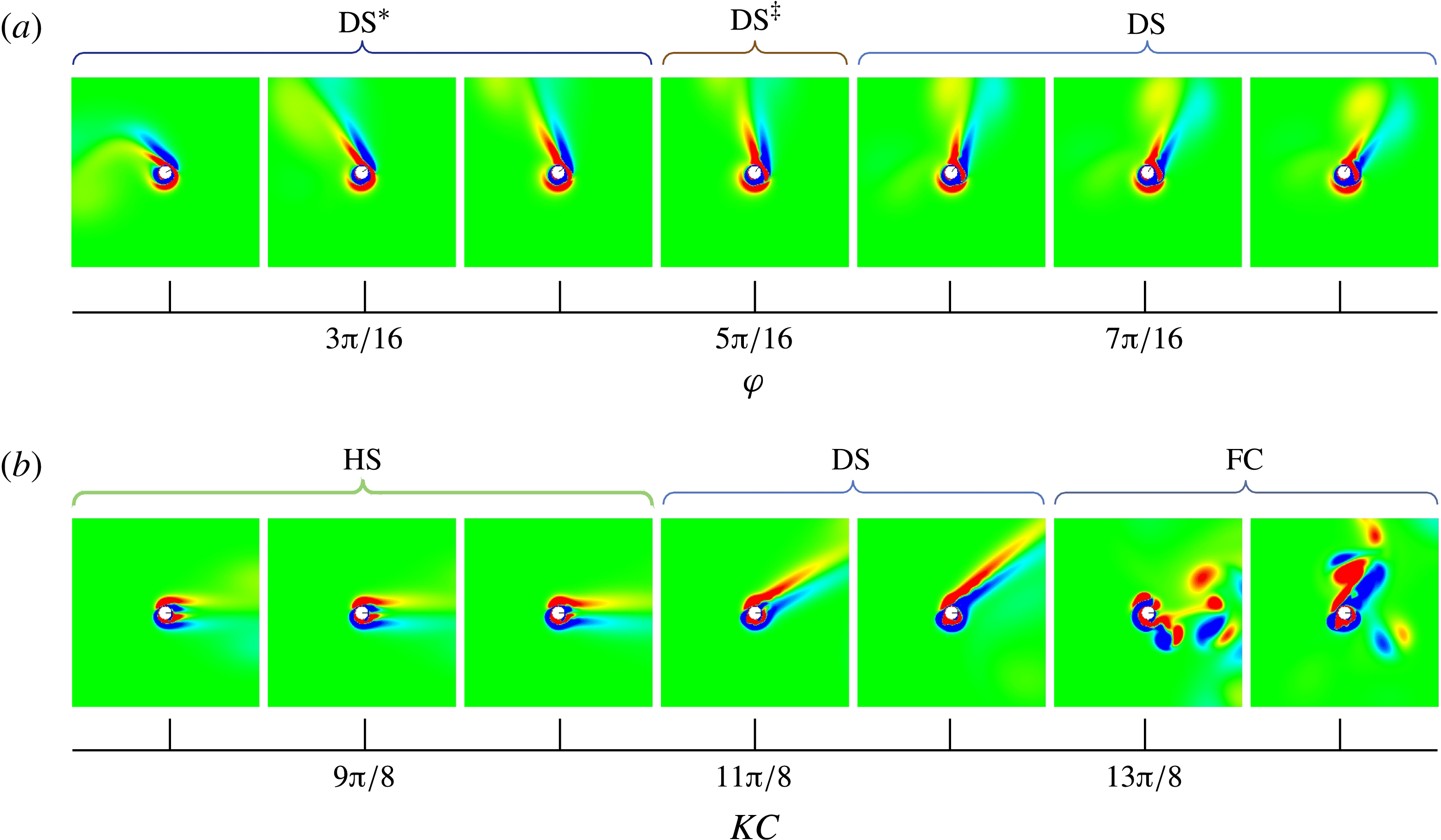
Another interesting trend that can be seen in figure 10 is the grouping of streaming flow regimes, particularly at lower Reynolds numbers. Upon zooming in and looking at the actual flow structures, one can see gradual changes in the deflection angle of the streaming jet flows occurring through slight variations in
 ${\it\varphi}$
and
 $\mathit{KC}$
. Two examples of this are shown in figure 11(a,b). Larger versions of the visualizations in figure 11 are included in supplementary figures 1–6, along with many other examples of the same phenomenon.
Colour-mapped instantaneous vorticity illustrating deflection angle transitions in streaming jet flows. (a) Gradual changes in the phase shift yielding a transition between
 $\text{DS}^{\ast }$
,
 $\text{DS}^{\ddagger }$
and DS flows when
 $\mathit{KC}={\rm\pi}$
and
 $\mathit{Re}=40{\rm\pi}$
. (b) Gradually increasing the Keulegan–Carpenter number in the completely out-of-phase case (
 ${\it\varphi}={\rm\pi}$
) yields DS flows before going chaotic. This example was run with
 $\mathit{Re}=50{\rm\pi}$
, but the same result was observed at many Reynolds numbers (figure 10
e).
It was previously shown by Blackburn et al. (Reference Blackburn, Elston and Sheridan1999) that one specific HS flow (
 $\mathit{KC}={\rm\pi}$
,
 $\mathit{Re}=90{\rm\pi}$
and
 ${\it\varphi}={\rm\pi}$
) yielded a net thrust force on the cylinder, which was capable of accelerating it to 33 % of its maximum translational velocity. Upon running this same case with prescribed kinematics, it was found that the time-averaged thrust coefficient was 0.2104. In order to determine if the directionality of the net force can be controlled, a dense series of time-averaged lift and drag coefficient measurements,
 $\bar{C}_{L}$
and
 $\bar{C}_{D}$
, were made in a portion of the state space that was known to contain a bifurcation from the HS regime to the DS regime (figure 11
b). The results of this study are plotted in figure 12.
Plot of the time-averaged lift and drag coefficients at a point in the state space where a bifurcation from the HS regime to the DS regime occurs when
 $\mathit{KC}$
is increased. In this case
 ${\it\varphi}={\rm\pi}$
and
 $\mathit{Re}=50{\rm\pi}$
. These data demonstrate the fact that the net force direction can be altered through subtle parameter changes.

In total, 58 simulations were run with
 ${\rm\pi}/128$
increments to
 $\mathit{KC}$
for each successive run. At lower
 $\mathit{KC}$
values, there is no net lift being produced. As
 $\mathit{KC}$
is increased, the net drag coefficient becomes increasingly negative as the jet strength increases. There is a relatively abrupt bifurcation in the state space from the HS regime to the DS regime when
 $\mathit{KC}$
approaches
 $11{\rm\pi}/8$
. At this point there is a clear decrease in the net lift coefficient as the jet begins to deflect in the anticlockwise direction. As
 $\mathit{KC}$
is increased further, both the time-averaged lift and drag coefficients continue to decrease.
The fact that slight parameter variations are capable of altering the direction of the force on the cylinder opens the door for using these flow regimes as a low-Reynolds-number propulsive alternative to flapping wings. This is desirable because the two-degree-of-freedom actuator necessary to make parameter tweaks to
 ${\it\varphi}$
and
 $\mathit{KC}$
for an oscillating cylinder would be simple compared to what is required to control multiple flapping wing systems. In the future we plan to incorporate fluid–structure interaction into this problem and look at the propulsive efficiency of flows in the DS regime. It remains to be seen if all the force-producing streaming jet flows will still form if the cylinder is allowed to move freely in the fluid. However, this is beyond the scope of the current work and will be investigated in a future study.
6. Discussion and conclusion
A detailed look at the flows induced by a circular cylinder undergoing oscillatory rotation and translation in a quiescent fluid has been presented. A broad parameter study was done in order to help identify potentially useful flow regimes. The parametric study was performed on the Reynolds number, Keulegan–Carpenter number and the phase shift between the rotational and translational harmonic motion.
There are several novel aspects of this work. To the best of our knowledge, the deflected streaming regimes (DS,
 $\text{DS}^{\ddagger }$
and
 $\text{DS}^{\ast }$
), the horizontal vortex shedding regime (HV), the jet transition regime (JT) and the double dipole regime (DD) have not been reported before. Also, the ability to alter the direction of the HS and DS jet flows with subtle parameter changes has not previously been demonstrated. It was shown that the deflected jets do in fact yield a net directional force on the cylinder. This demonstrates the potential of using these streaming jet flows as a propulsive mechanism that is controllable with a simple two-degree-of-freedom actuator.
6.1. Stability in three dimensions
While the two-dimensional point of view can shed light on important processes in low-Reynolds-number unsteady flows, it is important to ascertain how well the observed structures hold up in three dimensions. Some initial work has been done to that end. Specifically, a large three-dimensional simulation was carried out using dimensionless parameter values that are known to yield the DV flow regime (
 $\mathit{KC}={\rm\pi}$
,
 $\mathit{Re}=90{\rm\pi}$
and
 ${\it\varphi}=3{\rm\pi}/4$
). The grid used in this simulation was structurally the same as grid
 $G_{4}$
, although the size of individual grid blocks was slightly decreased such that
 $N_{d}=96$
. The length of the cylinder in the spanwise direction was
 $8D$
and periodic boundary conditions were applied at the spanwise domain boundaries. The case was run for 30 oscillations. The resulting flow at the end of the last translational oscillation is shown in figure 13. The general structure of the three-dimensional flow retains the wake deflection characteristic of the two-dimensional solution, despite the presence of spanwise periodicity.
Vorticity magnitude isosurfaces illustrate the flow structure from a three-dimensional simulation using dimensionless parameter values that produced the DV flow that was analysed in § 5.2 (
 $\mathit{KC}={\rm\pi}$
,
 $\mathit{Re}=90{\rm\pi}$
and
 ${\it\varphi}=3{\rm\pi}/4$
). Colour is mapped to the
 ${\it\omega}_{z}$
vorticity component. (a) Orthographic projection perpendicular to the spanwise axis showing horseshoe-shaped vortices in the deflected wake. (b) Orthographic projection along the spanwise axis showing that the deflection angle is similar to the two-dimensional case.

This suggests that the structure of the low-
 $\mathit{Re}$
flows detailed in § 5 will translate to three-dimensional space, especially since the majority of the new flow regimes occurred when
 $\mathit{Re}\leqslant 90{\rm\pi}$
(figure 10
b–e). However, more three-dimensional tests will need to be performed in the future with dimensionless parameters known to produce all the observed flow regimes, and stability analysis along the lines of those done by Nazarinia et al. (Reference Nazarinia, Jacono, Thompson and Sheridan2009b
) will need to be performed.
6.2. Similarities to aerofoil propulsion
As mentioned in the introduction, this work was motivated by the symmetry-breaking propulsive wakes observed behind oscillating aerofoils. In fact, the DV regime bears a striking resemblance to these deflected vortex streets. An analysis of the viscous surface stress distribution that leads to a shed dipole vortex pair during each oscillation in the DV regime was also presented, and there are additional parallels that can be drawn between the two problems. Specifically, tests were done to evaluate the long-term deflection angle behaviour in the DV and DS flow regimes.
In addition to Jones et al. (Reference Jones, Dohring and Platzer1998), several studies have investigated the temporal switching of the deflected jet angle. Heathcote & Gursul (Reference Heathcote and Gursul2004, Reference Heathcote and Gursul2007) observed that the near-field deflection angle changes periodically in time with a period two orders of magnitude greater than the aerofoil heaving period. They also observed that the switching period increased with increased foil stiffness. In a related study, Shinde & Arakeri (Reference Shinde and Arakeri2013) observed the long-time behaviour of the meandering jet to be random in time and not dependent on initial conditions. They opined that the leading-edge vortices observed in Heathcote & Gursul’s experiments could account for the differing results. It should be noted that the prescribed kinematics and aerofoil geometry differed between these studies. Wei & Zheng (Reference Wei and Zheng2013) investigated deflection angle changes between the near- and far-field wakes, concluding that they are due to a switch in vortex pairing patterns. Symmetry breaking and chaotic flows were also observed by Blondeaux, Guglielmini & Triantafyllou (Reference Blondeaux, Guglielmini and Triantafyllou2005) for aerofoils undergoing combined pitching and heaving and by Spagnolie et al. (Reference Spagnolie, Moret, Shelley and Zhang2010) for a prescribed heave and passive pitch motion.
Based on this literature, it is not exactly clear why different temporal switching behaviours of the jet deflection angle were observed in different studies. To gain a more general perspective, independent of aerofoil shape, on deflection angle behaviour at large times, one DV case and one
 $\text{DS}^{\ddagger }$
case were simulated to 2000 motion periods on a large grid (
 $G_{5}$
). When considering long-term wake deflection behaviour in the DS and DV regimes, the observed flows have three time scales. The smallest corresponds to the prescribed harmonic forcing of the cylinder. The intermediate scale corresponds to the formation of the deflected jet and its initial deflection angle. The potential periodic or random fluctuations in the deflection angle occur at the longest time scale (if at all), making this scale the most numerically onerous to capture.
For any given dimensionless parameter combination, it was found that the starting direction of the cylinder motion determined the deflection angle, which was then constant in time after settling down over the initial oscillations. Reversing the starting direction produced a mirrored deflected wake in both regimes, as can be seen in figures 5 c,d and 8 d,e. It should also be noted that, when employing a ‘soft’ instead of impulsive start, the wake would occasionally deflect in the opposite direction. The soft start was prescribed by weighting the rotational and translational dimensionless amplitudes based on the simulation time for the first several motion periods. We conjecture that the direction of the first oscillation with enough amplitude to make the formative flow bifurcate into the DV or DS regime varies as the number of motion periods employed in the soft start varies. For these reasons, we did not see any need to note specific deflection angle mirroring about the horizontal axis in the phase plots of figure 10.
With regard to jet switching, it should also be noted that the number of oscillations required for both DV and HV flows to ‘settle down’ varied with small dimensionless parameter fluctuations. Starting vortices re-entering the near field occasionally caused same signed vortices from neighbouring dipole pairs to roll up into a stronger vortex, which annihilated the local oppositely signed vortices and temporarily entrained the entire vortex street before being pushed into the far field (see supplementary movies 4 and 5). It is possible that similar phenomena are partially responsible for the varied results regarding wake deflection angle changes in aerofoils, but more research must be done on this topic.
6.3. Future work
There are several additional lines along which this work can be extended in the future. In particular, additional three-dimensional studies are needed to help further flush out the parameter space. Studies looking at the effects of turbulence, wall interaction or other flow disturbances on the formation of the observed regimes would also help gauge their persistence as propulsive mechanisms. Using optimization techniques to improve on the self-propulsive efficacy of the observed streaming jet flows is another potential extension to this work.
Acknowledgements
This work was supported in part by the Air Force Office of Scientific Research under Laboratory Tasks 09RB01COR (monitored by Dr Doug Smith) and 03VA01COR (monitored by Dr Fariba Fahroo), by HPTI and the DoD High Performance Computing Modernization Program through grant GS04T09DBC0017, and also by the National Science Foundation (award OCI-0904920).
Supplementary data
Supplementary data is available at http://dx.doi.org/10.1017/jfm.2014.699.



