1. Introduction
Comprehending the propagation of sound waves along the intake duct is vital for predicting the core characteristics of aircraft engine noise. Classical analyses typically assume an identical circular cross-section along the axis of the duct, consequently allowing for modelling using Bessel functions as the orthogonal basis functions (Rienstra & Hirschberg Reference Rienstra and Hirschberg2004). However, certain advanced aircraft designs, most notably next-generation blended wing body configurations, adopt deformed inlets to minimise drag, maximise ground clearance, optimise the pre-compression effects of the fuselage, or improve stealth performance.
Classification of the Wiener–Hopf technique research directions.

The study of wave equation solutions with elliptic boundary conditions dates back to early studies that utilised the elliptic coordinate system and Mathieu functions (McLachlan Reference McLachlan1947). Lowson & Baskaran (Reference Lowson and Baskaran1975) applied these tools to hard-wall straight ducts with elliptic cross-sections, theoretically studying the propagation of sound waves within the duct. Hong & Kim (Reference Hong and Kim1995) built upon this foundation, classifying modal patterns in elliptic ducts and elucidating the propagation rules of different modes along the axial direction of the duct. As a subsequent development, Oliveira & Gil (Reference Oliveira and Gil2014) replaced the hard-wall duct set-up with a lined-wall duct configuration. Most recently, Peake & Abrahams (Reference Peake and Abrahams2020) used the multiple scales method to derive the theoretical solution of sound propagation within ducts undergoing a geometrical transition from a circular cross-section to an elliptic cross-section along the axial direction. To the extent of our knowledge, theoretical models that reveal wave propagation and radiation emanating from elliptic ducts remain rare. This study bridges that gap by proposing an analytical model to tackle this problem.
In addition to studying the sound propagation within ducts, examining the wave scattering from an intake duct to its external environment is another important aspect of aircraft engine noise research. Such problems featuring mixed boundary conditions are well suited for utilising the Wiener–Hopf technique (Noble Reference Noble1958). Figure 1 shows the research directions of the Wiener–Hopf technique. The central step in applying this method involves factorising the kernel function into the product of two complex functions, which can be analysed separately in the positive and negative half-planes. Noble (Reference Noble1958) demonstrated the existence and uniqueness of this decomposition for scalar Wiener–Hopf kernels, and derived a theoretical calculation formula utilising the Cauchy integral method. This empowers us to tackle Wiener–Hopf problems involving scalar kernels.
The application of the Wiener–Hopf method in duct wave radiations was first proposed by Munt (Reference Munt1977) to tackle the scattering problem of semi-infinite straight pipes with hard-wall circular cross-sections. Rienstra (Reference Rienstra1984) later extended this method to a semi-infinite circular duct with a doubly infinite cylindrical hub. On top of this, Gabard & Astley (Reference Gabard and Astley2006) further proposed an analytical model for describing a duct set-up with a centre body, validating it against numerical simulation results, and conducting extensive parametric studies. In the interests of delving deeper into noise control methods, Demir & Rienstra (Reference Demir and Rienstra2006) further studied the model by including acoustic lining treatment on the wall. To address more complex scenarios involving annular cross-section pipes, researchers often simplify the problem by assuming an infinitely long central cylinder. To remove such a simplification, Veitch & Peake (Reference Veitch and Peake2008) extended this Wiener–Hopf method for modelling annular duct set-ups with semi-infinite coaxial cylinders. Overall, this modelling approach holds significant importance for comprehending noise scattering and suppression in turbofan engines.
For increasingly complicated aeroacoustic problems, the Wiener–Hopf kernel is generally not in scalar form, but in matrix form. When Ayton (Reference Ayton2016) studied the influence of the flat plate trailing edge extended by a poroelastic plate on plane wave scattering, she achieved the
 $3\times 3$
matrix form Wiener–Hopf kernel. Similarly, Kisil & Ayton (Reference Kisil and Ayton2018) proposed a theoretical solution method for the
 $2\times 2$
matrix kernel. In the field of pipe acoustics, the introduction of the matrix Wiener–Hopf kernel is often required when three-dimensional effects come into play due to circumferentially non-uniform boundary conditions. Liu et al. (Reference Liu, Jiang, Huang and Chen2016) introduced axially extended, circumferentially periodically distributed acoustic lining strips to study their impact on acoustic modal scattering in pipelines. Huang (Reference Huang2017) extended this contribution to the problem of plane wave scattering by a semi-infinite plate with a sawtooth trailing edge. Jiang, Lau & Huang (Reference Jiang, Lau and Huang2018) and Jiang & Huang (Reference Jiang and Huang2021) further studied the Wiener–Hopf model of a lined circular duct with arbitrary circumferentially lining distribution.
In this paper, we propose an analytical model for wave radiations from a semi-infinite elliptic duct in the presence of a uniform mean flow, as a model for forward noise emission in the next-generation blended wing body configurations. Our research builds upon and extends the framework established by Munt (Reference Munt1977), Rienstra (Reference Rienstra1984) and Gabard & Astley (Reference Gabard and Astley2006). The theoretical model describing the propagation of sound within elliptic ducts is inherited from Lowson & Baskaran (Reference Lowson and Baskaran1975) by using Mathieu functions. However, when addressing the scattering model for a semi-infinite elliptic duct, the problem becomes significantly more complex and cannot be resolved simply by replacing the Bessel functions with the Mathieu functions.
The well-established Wiener–Hopf method primarily focuses on radiation from circular or annular ducts, which can effectively be treated as a 2.5-dimensional problem (Zhang et al. Reference Zhang, Chen, Morfey and Nelson2004, Reference Zhang, Chen and Morfey2005; Huang et al. Reference Huang, Chen, Ma and Zhang2008), where the angular mode order
 $m$
is decoupled from the radial mode. Specifically, a circular mode with order
 $(m,n)$
can be expressed as
 \begin{equation} \varPsi _{1} = \cos (m\theta )\,\text{J}_m(\alpha _{\textit{mn}}r), \end{equation}
where
 $(r,\theta )$
are polar coordinates,
 $\text{J}_m$
denotes the
 $m$
th order Bessel function, and
 $\alpha _{\textit{mn}}$
represents the radial wavenumber. It is clear that its angular distribution is independent of the radial distribution. (The reverse, however, does not hold.) All scattered waves would also exhibit angular distribution
 $\cos (m\theta )$
. By solving the special case at
 $\theta = 0$
, the solution for any other azimuthal angle can be easily determined. In this process, only one Wiener–Hopf equation with a scalar kernel is involved.
On the other hand, an even-form elliptic mode can be written as
 \begin{equation} \varPsi _{2} = {\textit{ce}}_m(\eta ,q_{\textit{mn}})\,{\textit{Mc}}_m^{(1)}(\xi ,q_{\textit{mn}}), \end{equation}
where
 $(\xi ,\eta )$
are angular and radial variables from an elliptic coordinate system,
 ${\textit{ce}}_m$
and
 ${\textit{Mc}}_m^{(1)}$
are even-form angular and radial Mathieu functions, respectively, and
 $q_{\textit{mn}}$
is the parameter determined by rigid-wall boundary conditions. A detailed discussion of these variables and functions will be given in § 2. At this stage, the reader needs to know only that
 ${\textit{ce}}_m$
stands for the angular distribution,
 ${\textit{Mc}}_m^{(1)}$
refers to the radial distribution, and
 $q_{\textit{mn}}$
is a parameter related to the order of the angular and radial mode
 $(m,n)$
. The shared dependence of the angular and radial distributions on the parameter
 $q_{\textit{mn}}$
leads to their coupling. This coupling manifests itself as the three-dimensional effects in the radiation problems of elliptic ducts. At the duct lip, various radial distributions in the form of radial Mathieu functions are scattered from a single incident mode. Since they have different radial orders
 $n$
, their corresponding angular distributions also differ. As a result, it is no longer possible to use a two-dimensional axisymmetric model, as in the case of circular ducts, to describe the frequency-domain solution corresponding to any single incident mode. We will show later that this problem can ultimately be transformed into solving a set of Wiener–Hopf equations with scalar kernels.
The proposed analytical model is not merely a straightforward extension of Munt’s study on cylindrical ducts or a trivial replacement of Bessel functions with Mathieu functions. Instead, it introduces an innovative approach to tackling the inherent three-dimensional effects caused by the non-axisymmetric nature of elliptic ducts. Specifically, we employ a novel series expansion method in the Hilbert space using angular Mathieu functions as basis functions. This method overcomes the challenges posed by the elliptic geometry, transforming the radiation problem into the solution of a set of Wiener–Hopf equations with scalar kernels – a significant departure from the cases in cylindrical geometries. While Lowson & Baskaran (Reference Lowson and Baskaran1975) laid the groundwork for elliptic mode derivation, our work integrates and extends these results into a comprehensive framework tailored for scattering and radiation problems. The complexity of the geometry is not merely a matter of switching modal expansions; it fundamentally alters the problem structure. The coupling between angular and radial Mathieu functions introduces a level of mathematical intricacy that necessitates a more sophisticated treatment than the relatively decoupled modes in cylindrical ducts. The process of constructing Wiener–Hopf equations in our approach reflects these complexities and represents a valuable theoretical advancement for addressing non-axisymmetric duct acoustics.
The remaining part of this paper is organised as follows. Section 2 introduces the problem set-up. Section 3 develops the Wiener–Hopf model for this problem set-up. Next, numerical cases are executed in § 4 to validate the proposed theoretical model for sound radiations from an elliptic-shaped duct. Finally, § 5 summarises the key findings and contributions of this work.
2. Problem description
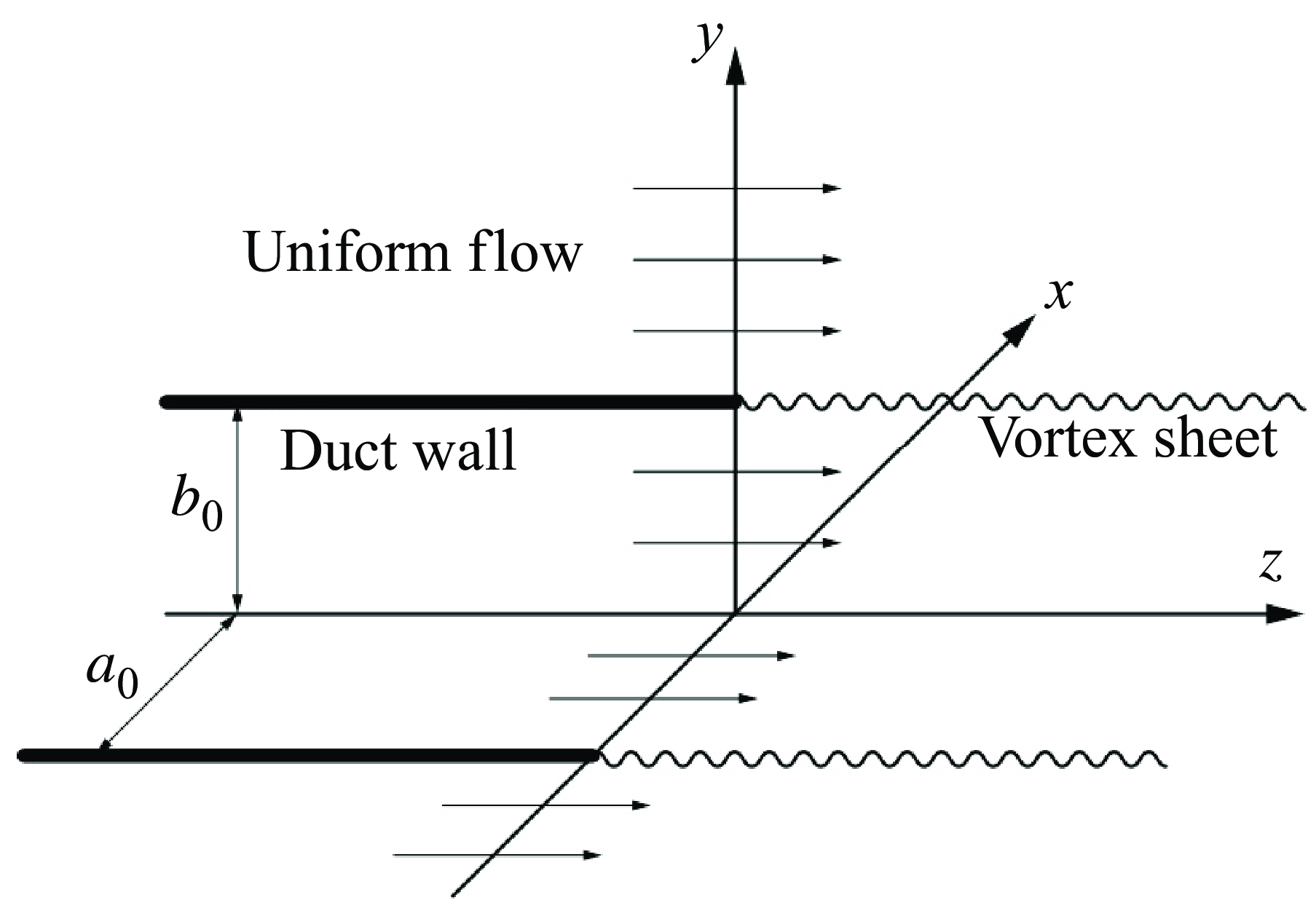
Consider a semi-infinite elliptic straight duct, depicted in figures 2 and 3, featuring a zero-thickness wall with semi-major axis length
 $a_0$
and semi-minor axis length
 $b_0$
. Then the foci are located at
 $(-h_0,0)$
and
 $(h_0,0)$
on the
 $x$
–
 $y$
plane, where
 \begin{equation} h_0 = \sqrt {a_0^2-b_0^2}. \end{equation}
The duct accommodates an axial uniform flow
 $v_0$
adhering to the ideal gas assumption for both its interior and exterior regions. In this analysis, we focus on cases where elliptic ducts function as inlets, implying that
 $v_0$
is generally negative. Static and outlet cases, however, are also discussed for completeness. The mean density and speed of sound are
 $\rho _0$
and
 $c_0$
, respectively.
Sketch of a semi-infinite straight duct with an elliptic cross-section.

Cross-sections of the model set-up on the
 $x$
–
 $z$
and
 $y$
–
 $z$
planes.

2.1. Elliptic-cylindrical coordinate system
In three-dimensional Euclidean space, the so-called elliptic-cylindrical coordinate system is an orthogonal coordinate system generated by projecting the two-dimensional elliptic coordinate system along the perpendicular
 $z$
-axis. The two-dimensional elliptic coordinate system, as shown in figure 4, consist of ellipses and hyperbolas with coincident foci
 $F_1$
and
 $F_2$
at
 $(-h_0,0)$
and
 $(h_0,0)$
, respectively. The definition of the elliptic-cylindrical coordinates
 $(\xi ,\eta ,\tilde {z})$
is then given by
 \begin{equation} \left \{\!\! \begin{array}{l} \tilde {x} = h_0 \cosh \xi \cos \eta , \\ \tilde {y} = h_0 \sinh \xi \sin \eta , \\ \tilde {z} = \tilde {z}, \end{array} \right . \end{equation}
where
 $\xi$
is non-negative real, and
 $-\unicode{x03C0} \lt \eta \leqslant \unicode{x03C0}$
. With the definition (2.2), all confocal ellipses could be expressed as
 $\xi = \textrm {constant}$
. Assuming that
 $\xi = \xi _0$
refers to the duct wall, we obtain
 \begin{equation} \xi _0 = \text{arctanh}\left (\frac {b_0}{a_0}\right )\!. \end{equation}
The two-dimensional elliptic coordinate system, where the thin solid lines and dotted lines are elliptic and hyperbolic coordinate lines, respectively. The thick solid line represents the cross-section of the duct wall, which is an ellipse with semi-major axis
 $a_0=0.5$
m and semi-minor axis
 $b_0=0.3$
m.

2.2. Governing equations
By making the spatial dimensions
 $\{\tilde {x}, \tilde {y}, \tilde {z}\}$
, mean velocity
 $v_0$
, acoustic density
 $\tilde {\rho }$
, time
 $\tilde {t}$
, velocity potential
 $\tilde {\phi }$
, and acoustic pressure
 $\tilde {p}$
dimensionless on
 $h_0$
,
 $c_0$
,
 $\rho _0$
,
 $h_0/c_0$
,
 $h_0c_0$
and
 $c_0^2\rho _0$
, respectively, the convected wave equation for velocity potential
 $\phi$
is
 \begin{equation} \left (\frac {\partial }{\partial t}+M\frac {\partial }{\partial z}\right )^2\phi - \Delta \phi = 0, \end{equation}
where
 $M = v_0/c_0$
, and
 $\Delta$
is the three-dimensional Laplace operator with respect to the dimensionless spatial variables
 $x$
,
 $y$
and
 $z$
. By taking the elliptic-cylindrical coordinates (2.2), (2.4) is extended as
 \begin{equation} \left (\frac {\partial }{\partial t}+M\frac {\partial }{\partial z}\right )^2\phi - \left [\frac {2}{\cosh 2\xi - \cos 2\eta }\left (\frac {\partial ^2 \phi }{\partial \xi ^2}+\frac {\partial ^2 \phi }{\partial \eta ^2}\right )+\frac {\partial ^2 \phi }{\partial z^2}\right ] = 0. \end{equation}
From the velocity potential, we can obtain the acoustic pressure
 $p$
, the particle velocity
 $\boldsymbol{v}=(v_\xi ,v_\eta ,v_z)$
and the acoustic density
 $\rho$
as
 \begin{equation} p = -\left (\frac {\partial }{\partial t}+M\frac {\partial }{\partial z}\right )\phi ,\quad \boldsymbol{v} = \boldsymbol{\nabla }\phi ,\quad \rho = p, \end{equation}
where
 $\boldsymbol{\nabla}$
denotes the gradient operator with respect to
 $\xi$
,
 $\eta$
and
 $z$
. The continuity of the acoustic pressure and particle velocity across the line segment connecting the two foci
 $F_1$
and
 $F_2$
yields
 \begin{equation} \left (\frac {\partial }{\partial t}+M\frac {\partial }{\partial z}\right )\phi (0,\eta ,z,t) = \left (\frac {\partial }{\partial t}+M\frac {\partial }{\partial z}\right )\phi (0,-\eta ,z,t), \ \forall z, \end{equation}
and
 \begin{equation} \frac {\partial }{\partial \xi }\phi (0, \eta , z, t) = -\frac {\partial }{\partial \xi }\phi (0, -\eta , z, t), \ \forall z, \end{equation}
respectively. The natural boundary conditions (2.7) and (2.8) differ from previous conditions in a traditional circular duct because the radial variable
 $\xi =0$
represents a line segment rather than a point, as it does in a circular duct.
The total acoustic field can be expressed as the summation of incident wave
 $\psi _i$
and scattered wave
 $\psi _s$
, which indicates
 \begin{equation} \phi (\xi ,\eta ,z,t) = [\psi _i(\xi ,\eta ,z)+\psi _s(\xi ,\eta ,z)]\exp (-\textrm {i}\omega t). \end{equation}
2.3. Sound propagating inside an elliptic duct
To solve for the incident wave
 $\psi _i$
, we first need to understand the characteristics of sound propagation within an elliptic duct. Following Lowson & Baskaran (Reference Lowson and Baskaran1975), for the acoustic velocity potential field inside the duct, we assume
 \begin{equation} \phi (\xi ,\eta ,z,t) = \varPhi _\xi (\xi )\,\varPhi _\eta (\eta )\,\varPhi _z(z)\exp (-\textrm {i}\omega t). \end{equation}
Substituting (2.10) into (2.5), we obtain
 \begin{align} \frac {2}{\cosh 2\xi - \cos 2\eta } \left (\frac {1}{\varPhi _\xi }\frac {\textrm {d}^2 \varPhi _\xi }{\textrm {d} \xi ^2} + \frac {1}{\varPhi _\eta }\frac {\textrm {d}^2 \varPhi _\eta }{\textrm {d} \eta ^2}\right ) + 4q &= 0, \end{align}
 \begin{align} \frac {1}{\varPhi _z}\frac {\textrm {d}^2 \varPhi _z}{\textrm {d} z^2} - \frac {1}{\varPhi _z}\left (-\textrm {i}\omega +M\frac {\textrm {d}}{\textrm {d} z}\right )^2\varPhi _z - 4q &= 0, \\[9pt] \nonumber \end{align}
where
 $q$
is a constant arising naturally from the process of separation of variables. Equation (2.11) will be used later to calculate the modal patterns across the elliptic duct cross-section, and (2.12) is the characteristic equation that governs the axial propagation. At this stage, we are dealing with a non-spinning elliptic mode propagating inside the duct. This means that we should obtain a standing wave solution rather than a travelling wave solution in both the azimuthal and radial directions. Therefore, the solution to (2.11), which corresponds to the solution of the angular and radial Mathieu equations, should be real. Given the relationship between the Mathieu function and its parameter
 $q$
,
 $q$
should be non-negative real.
For (2.11), the separation of
 $\varPhi _\xi$
and
 $\varPhi _\eta$
yields the following two equations: the classical forms of the angular Mathieu differential equation
 \begin{equation} \frac {\textrm {d}^2\varPhi _\eta }{\textrm {d}\eta ^2} + (a - 2q\cos 2\eta ) \varPhi _\eta = 0, \end{equation}
and the radial Mathieu differential equation
 \begin{equation} \frac {\textrm {d}^2\varPhi _\xi }{\textrm {d}\xi ^2} - (a - 2q\cosh 2\xi ) \varPhi _\xi = 0, \end{equation}
where
 $a$
is the eigenvalue derived from the recurrence relations (Appendix A; see Berezman et al. (Reference Berezman, Kerimov, Skorokhodov and Shadrin1986) for details).
The general solutions of (2.13) and (2.14) with four arbitrary constants
 $C_1$
,
 $C_2$
,
 $C_3$
and
 $C_4$
are
 \begin{align} \varPhi _\eta (\eta ) &= C_1{\textit{ce}}_m(\eta ,q) + C_2{\textit{se}}_m(\eta ,q), \end{align}
 \begin{align} \varPhi _\xi (\xi ) &= C_3{\textit{Mc}}^{(1)}_m(\xi ,q) + C_4{\textit{Ms}}^{(1)}_m(\xi ,q), \end{align}
where
 $m$
is the acoustic mode number along the angular direction
 $\eta$
, which will take a non-negative integer (for
 $C_2,C_4 = 0$
) or positive integer (for
 $C_2,C_4 \neq 0$
) to satisfy the circumferential periodicity condition,
 ${\textit{ce}}_m$
and
 ${\textit{se}}_m$
are angular Mathieu functions of even and odd form, respectively, and
 ${\textit{Mc}}^{(1)}_m$
and
 ${\textit{Ms}}^{(1)}_m$
are first-kind radial Mathieu functions of even and odd form, respectively. The normalisation of Mathieu functions follows the convention described in McLachlan (Reference McLachlan1947). Because of the physical constraints in this problem, the radial variable
 $\xi$
will be non-negative real.
The angular Mathieu functions
 ${\textit{ce}}_m(\eta ,q)$
and
 ${\textit{se}}_m(\eta ,q)$
can be classified as those in table 1. Note that
 ${\textit{se}}_0(\eta ,q)$
is undefined, and the angular distribution of a plane wave modal pattern can be expressed simply by using
 ${\textit{ce}}_0(\eta ,q)$
.
Classification of angular Mathieu functions by the parity and periodicity with respect to argument
 $\eta$
, where
 $l = 0,1,2,\ldots$
and
 $q$
is the parameter.

Assume
 $\varPsi (\xi ,\eta ) = \varPhi _\eta (\eta )\,\varPhi _\xi (\xi )$
. The continuity conditions (2.7) and (2.8) yield
 \begin{align} \varPsi (0, \eta ) - \varPsi (0, -\eta ) &= 0, \quad \forall \eta , \end{align}
 \begin{align} \frac {\partial }{\partial \xi } \varPsi (0, \eta ) + \frac {\partial }{\partial \xi } \varPsi (0, -\eta ) &= 0, \quad \forall \eta . \end{align}
Substitute (2.17) and (2.18) into (2.15) and (2.16). Considering the oddness of
 ${\textit{Ms}}^{(1)}_m$
and
 ${\textit{se}}_m$
and the evenness of
 ${\textit{Mc}}^{(1)}_m$
and
 ${\textit{ce}}_m$
, we obtain
 \begin{align} C_2C_3\, {\textit{Mc}}^{(1)}_m(0,q) {\textit{se}}_m(\eta ,q) - C_2C_3\, {\textit{Mc}}^{(1)}_m(0,q) {\textit{se}}_m(-\eta ,q) &= 0,\quad \forall \eta , \end{align}
 \begin{align} C_1C_4\, {{\textit{Ms}}^{(1)}_m}'(0,q) {\textit{ce}}_m(\eta ,q) + C_1C_4\, {{\textit{Ms}}^{(1)}_m}'(0,q){\textit{ce}}_m(-\eta ,q) &= 0,\quad \forall \eta , \end{align}
where
 $({\cdot })'$
denotes the derivative of a radial Mathieu function with respect to its argument
 $\xi$
. Hence
 $C_2C_3 = C_1C_4 = 0$
, and the general solution, with arbitrary complex constants
 $A_m = C_1C_3$
,
 $B_m = C_2C_4$
, is
 \begin{equation} \varPsi (\xi ,\eta ) = A_m\,{\textit{Mc}}_m^{(1)}(\xi ,q){\textit{ce}}_m(\eta ,q) + B_m{\textit{Ms}}_m^{(1)}(\xi ,q){\textit{se}}_m(\eta ,q). \end{equation}
Representative elliptic duct mode patterns. The Cartesian coordinates
 $(x,y)$
has been made dimensionless on half-focal length
 $h_0=0.4$
m. The solid line represents the cross-section of the duct wall, which is an ellipse with semi-major axis
 $a_0=0.5$
m and semi-minor axis
 $b_0=0.3$
m.

Now consider the boundary conditions on the duct wall:
 \begin{equation} \frac {\partial }{\partial \xi }\varPsi (\xi _0, \eta ) = 0, \quad \forall \eta . \end{equation}
Substitution of (2.21) into (2.22) yields
 \begin{equation} A_m\,{{\textit{Mc}}^{(1)}_m}'(\xi _0,q){\textit{ce}}_m(\eta ,q) + B_m{{\textit{Ms}}^{(1)}_m}'(\xi _0,q){\textit{se}}_m(\eta ,q) = 0, \quad \forall \eta . \end{equation}
A set of non-trivial linearly independent solutions can be found by taking either
 \begin{equation} {{\textit{Mc}}^{(1)}_m}'(\xi _0,q) = 0, \quad \text{with }B_m = 0, \end{equation}
or
 \begin{equation} {{\textit{Ms}}^{(1)}_m}'(\xi _0,q) = 0, \quad \text{with }A_m = 0. \end{equation}
Equations (2.24) and (2.25) should be solved individually, and the solution
 $q_{\textit{mn}}$
refers to the
 $(n-1)$
th non-negative real value that satisfies its corresponding wall boundary conditions. It is clear that
 $q_{\textit{mn}}$
, the solution of boundary conditions (2.24) or (2.25), can only be non-negative real, considering the Mathieu function calculation process described in Appendix A. We should note that the solutions of (2.24) and (2.25) are usually not identical. The value of
 $q_{\textit{mn}}$
determines which one of the linearly independent terms in (2.21) should be kept. Without loss of generality, we discuss only the elliptic modes of even form. By taking
 $A_m = 1$
and
 $B_m = 0$
, we can express the velocity potential distribution of an elliptic mode of even form as
 \begin{equation} \varPsi _{\textit{mn}}(\xi ,\eta ) = {\textit{Mc}}^{(1)}_m(\xi ,q_{\textit{mn}})\,{\textit{ce}}_m(\eta ,q_{\textit{mn}}). \end{equation}
Modal patterns
 $\varPsi _{\textit{mn}}$
with low angular and radial modal order are shown in figure 5.
Substituting
 $q = q_{\textit{mn}}$
into (2.12), the dimensionless axial wave number for the elliptic duct mode
 $(m,n)$
is related to
 $q_{\textit{mn}}$
by the dispersion relation
 \begin{equation} \mu _{\textit{mn}}^\pm = \frac {\pm \sqrt {1-4q_{\textit{mn}}(1-M^2)/\omega ^2} - M}{1-M^2}, \quad 0\lt \xi \lt \xi _0. \end{equation}
Note that since (2.24) and (2.25) generally have distinct solutions, the even and odd modes of the same order
 $(m,n)$
propagate inside the elliptic duct with different axial wavenumbers.
Hence the wave propagating inside the duct can be expressed as
 \begin{align} \phi (\xi ,\eta ,z,t) & = \sum _{m=0}^{+\infty } \sum _{n=0}^{+\infty } \left[A_{\textit{mn}}^- \exp \left(\textrm {i}\omega \mu _{\textit{mn}}^- z\right)+A_{\textit{mn}}^+ \exp \left(\textrm {i}\omega \mu _{\textit{mn}}^+ z\right)\right]\, \varPsi _{\textit{mn}}(\xi ,\eta )\exp (\rm -i\omega t),\nonumber\\& \quad 0\lt \xi \lt \xi _0, \end{align}
where
 $A_{\textit{mn}}^\pm$
are complex amplitudes. Since we are dealing with forward emissions from a semi-infinite duct, we set
 $A_{\textit{mn}}^-$
to zero, and keep only the sound waves propagating in the positive direction of the
 $z$
-axis. Now we can extract the incident wave
 $\psi _i$
from (2.28) as
 \begin{equation} \psi _i(\xi ,\eta ,z) = \left \{\!\! \begin{array}{ll} 0, &\xi \gt \xi _0, \\[4pt] A_{\textit{mn}}^+\,\varPsi _{\textit{mn}}(\xi ,\eta )\exp \left(\textrm {i}\omega \mu _{\textit{mn}}^+ z\right), &0\lt \xi \lt \xi _0. \end{array} \right . \end{equation}
2.4. Scattered wave
For the acoustic field scattered by the incident wave at the duct lip, we also assume
 \begin{equation} \psi _s(\xi ,\eta ,z,t) = \psi _s(\xi ,\eta ,z)\exp (-\textrm {i}\omega t), \end{equation}
and define the half-range Fourier transforms
 \begin{align} \beta _-(\xi ,\eta ,u) &= \int _{-\infty }^{0}\psi _s(\xi ,\eta ,z)\exp (-\textrm {i}\omega u z)\,\textrm {d}z, \end{align}
 \begin{align} \beta _+(\xi ,\eta ,u) &= \int _{0}^{+\infty }\psi _s(\xi ,\eta ,z)\exp (-\textrm {i}\omega u z)\,\textrm {d}z, \end{align}
where
 $u$
is the dimensionless axial wavenumber. The conventional Fourier transform is then obtained by simply taking
 \begin{equation} \beta (\xi ,\eta ,u) = \beta _-(\xi ,\eta ,u) + \beta _+(\xi ,\eta ,u). \end{equation}
The scattered wave (2.30) is also governed by (2.5). Substituting (2.30) into (2.5) and performing the Fourier transform (2.33), we obtain
 \begin{equation} \frac {2}{\cosh 2\xi - \cos 2\eta } \left (\frac {\partial ^2 \beta }{\partial \xi ^2}+\frac {\partial ^2 \beta }{\partial \eta ^2}\right ) + \omega ^2 \lambda ^2 \beta = 0, \end{equation}
where
 \begin{equation} \lambda ^2 = (1-uM)^2-u^2, \end{equation}
for
 $\lambda = \lambda _- \lambda _+$
with
 $\lambda _\pm =[1-u(M\pm 1)]^{1/2}$
. By taking the principal branches of the square root function, it could be derived that
 $\lambda _\pm$
go from
 $u_\pm$
to
 $\pm \infty$
, respectively, where
 $u_\pm = 1/(M\pm 1)$
.
We treat the axial wavenumber
 $u$
as a parameter, and then perform the variable separation
 \begin{equation} \beta (\xi ,\eta ,u) = \beta _\xi (\xi ,u)\, \beta _\eta (\eta ,u). \end{equation}
The applicability of variable separation is related not only to the coordinate system but also to the differential operators involved. Several related studies (Lowson & Baskaran Reference Lowson and Baskaran1975; Peake & Cooper Reference Peake and Cooper2001; Oliveira & Gil Reference Oliveira and Gil2014) have shown that the separation of spatial variables in the wave equation under elliptic coordinates is feasible. Boyer, Kalnins & Miller (Reference Boyer, Kalnins and Miller1976) provided a more detailed mathematical explanation of this issue. Substitution of (2.36) into (2.34) yields the form of the angular Mathieu equation
 \begin{equation} \frac {\textrm {d}^2\beta _\eta }{\textrm {d}\eta ^2} +(A - 2Q\cos 2\eta ) \beta _\eta = 0, \end{equation}
and the radial Mathieu equation
 \begin{equation} \frac {\textrm {d}^2\beta _\xi }{\textrm {d}\xi ^2} -(A - 2Q\cosh 2\xi ) \beta _\xi = 0, \end{equation}
where
 $Q = \omega ^2 \lambda ^2 /4$
is a function of
 $u$
, and
 $A$
denotes the eigenvalues of the corresponding Mathieu functions, like
 $a$
in (2.13) and (2.14). Similar to the discussion in § 2.3, the solution of (2.37) and (2.38) with arbitrary parametric coefficients
 $B_{0,\kappa }(u)$
and
 $B_{1,\kappa }(u)$
is
 \begin{equation} \beta (\xi ,\eta ,u) = \left \{\!\! \begin{array}{ll} \sum _{\kappa =0}^{+\infty } B_{0,\kappa }(u)\,{\textit{Mc}}_\kappa ^{(3)}(\xi ,Q)\, {\textit{ce}}_\kappa (\eta ,Q), &\xi \gt \xi _0, \\[6pt] \sum _{\kappa =0}^{+\infty } B_{1,\kappa }(u)\,{\textit{Mc}}_\kappa ^{(1)}(\xi ,Q)\, {\textit{ce}}_\kappa (\eta ,Q), &0\lt \xi \lt \xi _0, \end{array} \right . \end{equation}
where
 ${\textit{Mc}}_\kappa ^{(k)}$
is the
 $k$
th-kind radial Mathieu function of even form with non-negative integer order
 $\kappa$
, and
 ${\textit{ce}}_\kappa$
is the angular Mathieu function of even form with the same order
 $\kappa$
. In a practical implementation, the above infinite series would be truncated to a finite dimension.
Physically, (2.39) shows that an incident wave will be scattered into various different radial and angular Mathieu modes from the open end of an elliptic duct. The corresponding amplitudes of each mode can be rigorously determined based on the theoretical solutions that are to be developed below. In (2.39), we make an assumption that the scattered field resulting from an incident elliptic mode of even form is solely described by even-form Mathieu functions. This assumption holds due to the orthogonality property of angular Mathieu functions (McLachlan Reference McLachlan1947). However, if the incident wave consists of both even-form and odd-form elliptic modes, then the scattered field should be expressed as a linear combination of both even-form and odd-form Mathieu functions.
From (2.39), we find that
 $\beta$
can be expressed as the infinite series of the angular Mathieu functions of integer order, i.e.
 \begin{equation} \beta (\xi ,\eta ,u) = \sum _{\kappa =0}^{+\infty }\hat {\beta }_\kappa (\xi ,u)\,{\textit{ce}}_\kappa (\eta ,Q). \end{equation}
By comparing (2.39) and (2.40), we express the coefficients
 $\hat {\beta }_\kappa$
in the form of matrix operation as
 \begin{equation} \hat {\beta }_\kappa (\xi ,u) = \left \{\!\! \begin{array}{ll} B_{0,\kappa }(u)\,{\textit{Mc}}_\kappa ^{(3)}(\xi ,Q), &\xi \gt \xi _0, \\[6pt] B_{1,\kappa }(u)\,{\textit{Mc}}_\kappa ^{(1)}(\xi ,Q), &0\lt \xi \lt \xi _0. \end{array}\right . \end{equation}
2.5. Boundary conditions
There are three possible forms of the uniform mean flow: completely stationary, in the positive
 $z$
-axis direction, or in the negative
 $z$
-axis direction. Accordingly, the semi-infinite elliptic duct would be an ordinary duct, an outlet duct, or an inlet duct. It is important to note that the vortex sheet shown in figure 3 truly exists only in the second scenario, where the semi-infinite elliptic duct is used as an outlet duct. For the first and third scenarios, where the semi-infinite elliptic duct is used as an ordinary duct or an inlet duct, the vortex sheet is merely used to establish the necessary boundary conditions between the inner and outer sides.
The radial displacement of the sound particles on the vortex sheet is defined as
 \begin{equation} w(\eta ,z,t) = w(\eta , z)\exp (-\textrm {i}\omega t). \end{equation}
Omitting the time harmonic factor
 $\exp (-\textrm {i}\omega t)$
, particle displacement
 $w(\eta ,z)$
on the vortex sheet is related to the particle velocity as
 \begin{align} \left (-\textrm {i}\omega + M\frac {\partial }{\partial z}\right )w(\eta ,z) &= \frac {\partial }{\partial \xi }\psi _s\left(\xi _0^+, \eta , z\right), \quad \xi \gt \xi _0, \quad z\gt 0, \end{align}
 \begin{align} \left (-\textrm {i}\omega +M\frac {\partial }{\partial z}\right )w(\eta ,z) &= \frac {\partial }{\partial \xi }\psi _s\left(\xi _0^-, \eta , z\right), \quad 0\lt \xi \lt \xi _0, \quad z\gt 0, \end{align}
where the two limiting variables
 $\xi _0^+$
and
 $\xi _0^-$
approach
 $\xi _0$
from the positive and negative directions, respectively.
Readers may notice that (2.43) and (2.44) appear to be physically incorrect. The right-hand sides do not represent dimensionless particle velocity since the radial coordinate base
 $\partial _\xi$
is not a unitary base. To address this issue arising from coordinate transformations, we must note that in (2.42), (2.43) and (2.44), the particle displacement and velocity are expressed by their corresponding covariant components based on the local contravariant bases
 $(\partial _\xi ,\partial _\eta ,\partial _\zeta )$
. Due to the invariant nature of vector fields under changes in coordinate bases, these equations remain valid.
The continuity of the acoustic pressure across the vortex sheet yields
 \begin{equation} \left (\!-\textrm {i}\omega + M\frac {\partial }{\partial z}\right )\psi _s\left(\xi _0^+,\eta ,z\right) = \left (\!-\textrm {i}\omega + M\frac {\partial }{\partial z}\right )\! \left[\psi _s\left(\xi _0^-,\eta ,z\right)+\psi _i\left(\xi _0^-,\eta ,z\right)\right], \!\quad z\gt 0. \end{equation}
The boundary condition of the rigid duct wall is
 \begin{equation} \frac {\partial }{\partial \xi } \psi _s\left(\xi _0^-, \eta , z\right) = \frac {\partial }{\partial \xi } \psi _s\left(\xi _0^+, \eta , z\right) = 0, \quad z\leqslant 0. \end{equation}
3. Wiener–Hopf method
The Wiener–Hopf method is a powerful mathematical tool for solving two-dimensional partial differential equations with mixed boundary conditions. When encountering problems with three-dimensional effects, we usually need to introduce Fourier series to reduce the dimensionality of the problem (Liu et al. Reference Liu, Jiang, Huang and Chen2016; Huang Reference Huang2017; Jiang et al. Reference Jiang, Lau and Huang2018). Introducing the decomposition method analogous to the Fourier series comes at the cost of the Wiener–Hopf kernel function transforming into a matrix rather than a scalar. In this work, we leverage the unique properties of Mathieu functions, and introduce a decomposition method analogous to the Fourier series.
3.1. Wiener–Hopf equation
First, introduce the half-range Fourier transforms
 \begin{align} F_+(\eta ,u) &= \int _{0}^{+\infty } w(\eta ,z)\exp (-\textrm {i}\omega u z)\, \textrm {d}z, \end{align}
 \begin{align} G_-(\eta ,u) &= \int _{-\infty }^{0} \left (-\textrm {i}\omega + M\frac {\partial }{\partial z}\right )\left [\psi _s\left(\xi _0^+,\eta ,z\right)-\psi _s\left(\xi _0^-,\eta ,z\right)\right ] \exp (-\textrm {i}\omega uz)\, {\rm d}z, \end{align}
 \begin{align} G_+(\eta ,u) &= \int _{0}^{+\infty }\left (-\textrm {i}\omega + M\frac {\partial }{\partial z}\right )\left [\psi _s\left(\xi _0^+,\eta ,z\right)-\psi _s\left(\xi _0^-,\eta ,z\right)\right ] \exp (-\textrm {i}\omega uz)\,{\rm d}z, \end{align}
and the conventional Fourier transform
 \begin{equation} G(\eta ,u) = G_-(\eta ,u) + G_+(\eta ,u). \end{equation}
Note that
 \begin{equation} \psi _s\left(\xi _0^+,\eta ,z\right)-\psi _s\left(\xi _0^-,\eta ,z\right) = \psi _i(\xi _0,\eta ,z),\quad z\gt 0. \end{equation}
Therefore, by performing (3.3) on the incident wave (2.29), we obtain
 \begin{equation} G_+(\eta ,u) = A_{\textit{mn}}^+ \frac {1-\mu _{\textit{mn}}^+ M}{\mu _{\textit{mn}}^+ - u} {\textit{Mc}}_{m}^{(1)} (\xi _0,q_{\textit{mn}})\, {\textit{ce}}_m (\eta ,q_{\textit{mn}}). \end{equation}
Now we turn to the key part of this theoretical development. The implementation of the Wiener–Hopf method requires decoupling of the angular variable
 $\eta$
. To achieve this, we put forward an assumption, i.e. the distribution of almost all continuous and integrable periodic functions along the angular variable
 $\eta$
, e.g.
 $f(\eta )$
, can be decomposed in a method that imitates the Fourier series expansion. The basis function of this decomposition will be the angular Mathieu functions of integer orders with the same parameter, say
 $Q$
. Then
 $f(\eta )$
can be written in the series form
 \begin{equation} f(\eta ) = \sum _{\kappa =0}^{+\infty } \hat {f}_{c,\kappa }(\eta )\, {\textit{ce}}_\kappa (\eta ,Q) + \sum _{\kappa =1}^{+\infty } \hat {f}_{s,\kappa }(\eta )\, {\textit{se}}_\kappa (\eta ,Q). \end{equation}
The rationale behind our assumption is quite straightforward. The angular Mathieu functions of integer orders with the same parameter
 $Q$
can be expressed by Fourier series as (A1)–(A4). And for the
 $\kappa$
th-order angular Mathieu function
 ${\textit{ce}}_\kappa (\eta ,Q)$
or
 ${\textit{se}}_\kappa (\eta ,Q)$
, the complex amplitudes of its corresponding Fourier series form one of the linear independent eigenvectors derived from the recurrence relations (see Appendix A for more details), which means that in a Hilbert space, the angular Mathieu functions of integer orders with the same parameter
 $Q$
can also form a set of linearly independent basis functions. Actually, we can further prove the orthogonality conditions as follows (McLachlan Reference McLachlan1947):
 \begin{align} \int _{0}^{2\unicode{x03C0} }{\textit{ce}}_m(\eta ,Q)\,{\textit{ce}}_p(\eta ,Q)\,\textrm {d}\eta &= 0, \quad m\neq p, \quad m,p\ \text{non-negative integers}, \end{align}
 \begin{align} \int _{0}^{2\unicode{x03C0} }{\textit{se}}_m(\eta ,Q)\,{\textit{se}}_p(\eta ,Q)\,\textrm {d}\eta &= 0, \quad m\neq p, \quad m,p\ \text{positive integers}, \end{align}
 \begin{align} \int _{0}^{2\unicode{x03C0} }{\textit{ce}}_m(\eta ,Q)\,{\textit{se}}_p(\eta ,Q)\,\textrm {d}\eta &= 0, \quad m\neq p, \quad m,p\ \text{positive integers}. \end{align}
Equation (3.10) also suggests that considering only even modes does not lead to a loss of generality, since elliptic modes of even and odd form are linearly independent.
At this stage, it is important to clarify that the functions that we intend to decompose are not arbitrary. They all arise from an even-form elliptic mode as indicated by (2.29) within the context of this study. Utilising the orthogonality condition (3.10), we assert that only even-form Mathieu functions need be employed as basis functions for this decomposition, such as in the case of
 $G_+(\eta ,u)$
:
 \begin{equation} G_+(\eta ,u) = \sum _{\kappa =0}^{+\infty } \hat {G}_{+,\kappa }(u)\, {\textit{ce}}_\kappa (\eta ,Q). \end{equation}
Similarly, we have the series expansions of
 $G_-(\eta ,u)$
and
 $F_+(\eta ,u)$
as
 \begin{align} G_-(\eta ,u) &= \sum _{\kappa =0}^{+\infty } \hat {G}_{-,\kappa }(u)\, {\textit{ce}}_\kappa (\eta ,Q), \end{align}
 \begin{align} F_+(\eta ,u) &= \sum _{\kappa =0}^{+\infty } \hat {F}_{+,\kappa }(u)\, {\textit{ce}}_\kappa (\eta ,Q). \end{align}
Different from (3.11), where
 $G_+(\eta ,u)$
is already known in (3.6),
 $G_-(\eta ,u)$
and
 $F_+(\eta ,u)$
are unknown functions that need to be solved, and we can do so only by solving
 $\hat {F}_{+,\kappa }(u)$
first using the Wiener–Hopf method in the remaining part of this subsection.
By applying a Fourier transform along the axial direction
 $z$
to (2.43) and (2.44), we obtain
 \begin{align} -\textrm {i}\omega (1-uM)\,F_+(\eta ,u) &= \frac {\partial }{\partial \xi }\beta (\xi _0^+,\eta ,u), \quad \xi \gt \xi _0, \end{align}
 \begin{align} -\textrm {i}\omega (1-uM)\,F_+(\eta ,u) &= \frac {\partial }{\partial \xi }\beta (\xi _0^-,\eta ,u), \quad 0\lt \xi \lt \xi _0. \end{align}
Next, substitute the series (2.40) and (3.13) into (3.14) and (3.15). By comparing the coefficients, we obtain
 \begin{align} -\textrm {i}\omega (1-uM)\,\hat {F}_{+,\kappa }(u) &= {{\textit{Mc}}_\kappa ^{(3)'}}(\xi _0,Q)\, B_{0,\kappa }(u), \quad \xi \gt \xi _0, \end{align}
 \begin{align} -\textrm {i}\omega (1-uM)\,\hat {F}_{+,\kappa }(u) &= {{\textit{Mc}}_\kappa ^{(1)'}}(\xi _0,Q)\, B_{1,\kappa }(u), \quad 0\lt \xi \lt \xi _0. \end{align}
The continuity conditions across the vortex sheet (2.45) and the boundary condition of the rigid wall (2.46) yield
 \begin{equation} \hat {G}_{-,\kappa }(u) + \hat {G}_{+,\kappa }(u) = \textrm {i}\omega (1-uM) [{\textit{Mc}}_\kappa ^{(1)}(\xi _0,Q)\, B_{1,\kappa }(u) -{\textit{Mc}}_\kappa ^{(3)}(\xi _0,Q)\, B_{0,\kappa }(u)]. \end{equation}
Combining (3.16), (3.17) and (3.18), we obtain the Wiener–Hopf equation
 \begin{equation} \hat {G}_{-,\kappa }(u) + \hat {G}_{+,\kappa }(u) = K_\kappa (u)\, \hat {F}_{+,\kappa }(u), \end{equation}
where the Wiener–Hopf kernel is
 \begin{eqnarray} K_\kappa (u) = \omega ^2(1-uM)^2\left [\frac {{\textit{Mc}}_\kappa ^{(3)}(\xi _0,Q)}{{{\textit{Mc}}_\kappa ^{(3)'}}(\xi _0,Q)} - \frac {{\textit{Mc}}_\kappa ^{(1)}(\xi _0,Q)}{{{\textit{Mc}}_\kappa ^{(1)'}}(\xi _0,Q)}\right ]\!. \end{eqnarray}
3.2. Analytic strip and integration path
A unique solution requires an appropriate radiation condition that guarantees sound absorption at infinity. The Sommerfeld condition, which ensures that scattered waves radiate only outwards from known sources, is applied to maintain the causality of the initial value problem. Jones & Morgan (Reference Jones and Morgan1972) showed the proper approach by adding a positive imaginary component to the angular frequency
 $\omega$
. To mathematically describe the behaviour of acoustic waves radiating away to infinity, we introduce a complex angular frequency
 \begin{equation} \omega = |\omega |\exp (\textrm {i}\varepsilon ),\quad 0\leqslant \varepsilon \leqslant \frac {\unicode{x03C0} }{2}, \end{equation}
with
 $\varepsilon$
close to
 $\unicode{x03C0} /2$
, all waves decaying exponentially. Then we let
 $\varepsilon$
go to zero, the far-field radiation condition is correctly adopted, and the solution is obtained at a nearly real angular frequency. This process is vital for us to understand the behaviour of the Wiener–Hopf kernel function in the complex
 $u$
-plane, and gives us important insights into how to construct the analytical strip and integration path.
Schematics of the analytic strip and the integration path:
 $(a)$
when
 $\varepsilon$
is sufficiently large, the two complex half-planes
 $R_\pm$
define the overlapped strip
 $S$
with
 $M\lt 0$
;
 $(b)$
as
 $\varepsilon$
goes to 0, the analytic strip degenerates into a slightly deformed integration path that bypasses all possible acoustic zeros, poles and the aerodynamic zero
 $u_0$
.

To determine the analytical strip, it is necessary to discuss the regularity of
 $\beta (\xi ,\eta ,u)$
. As shown in figure 6
 $(a)$
, since
 $Q=\omega ^2\lambda ^2/4$
, the regularity conditions of the radial Mathieu functions require that
 $u$
can only take the value within the analytic strip defined by the half-planes
 $R_-$
and
 $R_+$
, where the half-planes
 $R_\pm$
are defined, respectively, as
 \begin{equation} \pm \textrm {Im}(u-u_\pm )\lt \mp \tan (\varepsilon )\,\text{Re}(u-u_\pm ). \end{equation}
As
 $\varepsilon \rightarrow 0$
, the integration path is slightly deformed around the aerodynamic double zero
 $u_0=1/M$
and the acoustic zeros and poles. Finally, as shown in figure 6
 $(b)$
, the analytic strip
 $S$
degenerates into the deformed integration path
 $\mathit \varGamma$
that goes from
 $-\infty +0\textrm {i}$
to
 $+\infty -0\textrm {i}$
and crosses the real axis at
 $u_c$
with
 \begin{equation} u_c = \frac {u_-+u_+}{2} = \frac {M}{M^2-1}. \end{equation}
For static cases with stationary flows,
 $M=u_c=0$
. For outlet cases,
 $M\gt 0$
, hence
 $u_c\lt 0$
. For inlet cases,
 $M\lt 0$
, hence
 $u_c\gt 0$
.
3.3. Kernel factorisation
Kernel factorisation is the key step in the implementation of the Wiener–Hopf technique. To clarify this procedure, we demonstrate the factorisation of
 $K_\kappa (u)$
. Detailed descriptions can be found in Munt (Reference Munt1977) and Rienstra (Reference Rienstra1984).
Before factorisng
 $K_\kappa (u)$
, we note that there are obvious aerodynamic double zeros associated with the Mach number of the uniform mean flow when
 $M\neq 0$
. These can be straightforwardly derived from (3.20) as
 \begin{equation} u_0 = \frac {1}{M}, \quad M\neq 0. \end{equation}
It would be beneficial to remove the possible double zeros prior to the factorisation of (3.20), which yields
 \begin{equation} K_\kappa (u) = \tilde {K}_\kappa (u)\,(u-u_0)^b, \end{equation}
where
 $b$
is an enumerable integer depending on the axial mean flow. For a static test case (
 $M=0$
), the aerodynamic zeros do not exist, hence
 $b=0$
. Otherwise, for the case with a uniform flow (
 $M\neq 0$
), we set
 $b=2$
.
Assume that
 $K_\kappa (u)$
is factorised into the form
 \begin{equation} K_\kappa (u) = \frac {K_{+,\kappa }(u)}{K_{-,\kappa }(u)}(u-u_0)^b, \end{equation}
with
 $K_{\pm ,\kappa }$
regular and non-zero on
 $R_\pm$
. Using Cauchy’s integration gives
 \begin{equation} \log K_{\pm ,\kappa }(u) = -\frac {1}{2\unicode{x03C0} \textrm {i}} \int _C \frac {\log [K_\kappa (\zeta )/(u-u_0)^b]}{\zeta -u}\,\textrm {d}\zeta . \end{equation}
As
 $\varepsilon \rightarrow 0$
, the integration path
 $C$
goes from
 $-\infty +i\varepsilon$
to
 $+\infty -i\varepsilon$
and crosses the real axis at
 $u_c=(u_-+u_+)/2$
. Since the integration path is symmetric about
 $u_c$
on the complex
 $u$
-plane, performing variable substitution and integrating along the new path gives
 \begin{align} \log K_{\pm ,\kappa }(u) &= -\frac {1}{2\unicode{x03C0} {\rm i}} \int _{0}^{+\infty -\textrm {i}\varepsilon }\left \{ \frac {\log [K_\kappa (u_c-v)/(u-u_0)^b]}{u_c-v-u} \right .\nonumber\\&\quad \left . +\, \frac {\log [K_\kappa (u_c+v)/(u-u_0)^b]}{u_c+v-u} \right \}\textrm {d}v, \end{align}
with
 \begin{equation} v(\mu ) = \left \{\!\! \begin{array}{ll} \mu + \textrm {i}\left (\frac {\Delta u - \varepsilon }{\Delta u^2}\mu ^2 -\mu \right ), & 0\leqslant \mu \lt \Delta u, \\ \mu - \textrm {i}\varepsilon , & \mu \geqslant \Delta u, \end{array} \right . \end{equation}
where
 $\Delta u = (u_+ - u_-)/2$
. For
 $K_{+,\kappa }(u)$
, if
 $u$
is above the integration contour, then we add the contributions of the pole
 $\zeta = u$
. In contrast, for
 $K_{-,\kappa }$
, a similar operation needs to be done when
 $u$
is below the integration contour.
3.4. General solutions
Substituting (3.26) into (3.19) gives
 \begin{equation} K_{+,\kappa }(u)\, \hat {F}_{+,\kappa }(u)\, (u-u_0)^b = K_{-,\kappa }(u)\,\hat {G}_{-,\kappa }(u) + K_{-,\kappa }(u)\,\hat {G}_{+,\kappa }(u). \end{equation}
By taking out the acoustic poles, we obtain
 \begin{align} &K_{+,\kappa }(u)\, \hat {F}_{+,\kappa }(u)\, (u-u_0)^b - K_{-,\kappa }\left(\mu _{\textit{mn}}^+\right)\, \hat {G}_{+,\kappa }(u) =K_{-,\kappa }(u)\,\hat {G}_{-,\kappa }(u) \nonumber \\ &\quad + \hat {G}_{+,\kappa }(u)\left[K_{-,\kappa }(u)-K_{-,\kappa }\left(\mu _{\textit{mn}}^+\right)\right]. \end{align}
The left- and right-hand sides of (3.31) are regular on the half-planes
 $R_\pm$
, respectively. According to analytic continuation in the complex analysis theory, (3.31) defines an entire function
 $E_\kappa (u)$
that is regular on the whole complex
 $u$
-plane.
3.4.1. Static cases
In the static flow case, there is no need to introduce the Kutta condition. It is necessary to discuss the behaviour of
 $E_\kappa (u)$
as
 $|u|\rightarrow \infty$
. The expansions of Mathieu functions in series of cross-products of Bessel functions (Appendix A) provide insightful details regarding
 $K_{\kappa }(u)$
, and ultimately lead to the inference that
 $K_{\pm ,\kappa }(u)\sim \textit {O}(u^{\mp 1/2})$
as
 $|u|\rightarrow \infty$
. For a static case (
 $M=0$
and
 $b=0$
), it is straightforward to assert
 $\psi _s(\xi _0,z)\sim \textit {O}(z)$
as
 $z\rightarrow 0$
. Following Noble (Reference Noble1958), this condition results in the conclusion that
 $F_{+,\kappa }(u)\sim \textit {O}(u^{-2})$
and
 $G_{-,\kappa }(u)\sim \textit {O}(u^{-1})$
as
 $|u|\rightarrow \infty$
, derived from (2.6), (3.1) and (3.19). Hence
 $E_\kappa (u)\sim \textit {O}(u^{-1/2})$
as
 $|u|\rightarrow \infty$
. Following Liouville’s theorem, the left-hand side of (3.31) is identically zero, i.e.
 \begin{equation} K_{+,\kappa }(u)\, \hat {F}_{+,\kappa }(u) - K_{-,\kappa }\left(\mu _{\textit{mn}}^+\right)\, \hat {G}_{+,\kappa }(u) = 0. \end{equation}
Hence
 \begin{equation} \hat {F}_{+,\kappa }(u) = K_{+,\kappa }^{-1}(u)\, K_{-,\kappa }\left(\mu _{\textit{mn}}^+\right)\, \hat {G}_{+,\kappa }(u). \end{equation}
3.4.2. Outlet cases
When the elliptic duct is used as a nozzle (given that we are only addressing uniform flow, this nozzle holds limited practical applicability), the full Kutta condition is applied at the duct lip, ensuring that all vortices shed exclusively from the lip. Note that the problem addressed in this study involves only uniform flow, unlike the work of Gabard & Astley (Reference Gabard and Astley2006), where instability waves form at the duct lip due to the velocity difference between the jet and the ambient flow, and propagate downstream. Therefore, flow instability and its effects are not considered in this study. For an outlet problem (
 $M\gt 0$
and
 $b=2$
), the velocity potential is a simple zero at the duct lip, which means
 $\psi _s(\xi _0,z)\sim \textit {O}(z^{3/2})$
as
 $z\rightarrow 0$
. Similarly, we have
 $F_{+,\kappa }(u)\sim \textit {O}(u^{-5/2})$
and
 $G_{-,\kappa }(u)\sim \textit {O}(u^{-3/2})$
as
 $|u|\rightarrow \infty$
. Hence
 $E_\kappa (u)\sim \textit {O}(u^{-1})$
as
 $|u|\rightarrow \infty$
, and (3.31) turns out to be
 \begin{equation} K_{+,\kappa }(u)\, \hat {F}_{+,\kappa }(u)\, (u-u_0)^2 - K_{-,\kappa } \big(\mu _{\textit{mn}}^+ \big)\, \hat {G}_{+,\kappa }(u) = 0. \end{equation}
Then
 \begin{equation} \hat {F}_{+,\kappa }(u) = \frac {K_{+,\kappa }^{-1}(u)\, K_{-,\kappa } \big(\mu _{\textit{mn}}^+ \big)\, \hat {G}_{+,\kappa }(u)}{(u-u_0)^2}. \end{equation}
3.4.3. Inlet cases
When the elliptic duct serves as an inlet, vortex shedding at the lip is considered non-physical, making the application of the Kutta condition unnecessary. For an inlet problem set-up (
 $M\lt 0$
and
 $b=2$
), the velocity potential is singular at the lip, which translates to
 $\psi _s(\xi _0,z)\sim \textit {O}(z^{1/2})$
as
 $z\rightarrow 0$
. Therefore, we can derive that
 $F_{+,\kappa }(u)\sim \textit {O}(u^{-3/2})$
and
 $G_{-,\kappa }(u)\sim \textit {O}(u^{-1/2})$
as
 $|u|\rightarrow \infty$
. Then
 $E_\kappa (u)\sim \textit {O}(1)$
as
 $|u|\rightarrow \infty$
, which implies that
 $E_\kappa (u)\equiv E_\kappa (u_0)$
. We obtain from (3.31) that
 \begin{equation} K_{+,\kappa }(u)\, \hat {F}_{+,\kappa }(u)\, (u-u_0)^2 - K_{-,\kappa }\left(\mu _{\textit{mn}}^+\right)\, \hat {G}_{+,\kappa }(u) = - K_{-,\kappa }\left(\mu _{\textit{mn}}^+\right)\, \hat {G}_{+,\kappa }(u_0). \end{equation}
Then
 \begin{equation} \hat {F}_{+,\kappa }(u) = \frac {K_{+,\kappa }^{-1}(u)\, K_{-,\kappa }\left(\mu _{\textit{mn}}^+\right)\, [\hat {G}_{+,\kappa }(u) - \hat {G}_{+,\kappa }(u_0)]}{(u-u_0)^2}. \end{equation}
3.4.4. Inverse Fourier transforms
On substituting
 $\hat {F}_{+,\kappa }(u)$
into (3.16) and (3.17), we get
 $B_{0,\kappa }(u)$
,
 $B_{1,\kappa }(u)$
solved respectively as
 \begin{align} B_{0,\kappa }(u) &= -\textrm {i}\omega (1-uM) \frac {\hat {F}_{+,\kappa }(u)}{{{\textit{Mc}}_\kappa ^{(3)'}}(\xi _0,Q)},\quad \xi \gt 0, \end{align}
 \begin{align} B_{1,\kappa }(u) &= -\textrm {i}\omega (1-uM) \frac {\hat {F}_{+,\kappa }(u)}{{{\textit{Mc}}_\kappa ^{(1)'}}(\xi _0,Q)},\quad 0\lt \xi \lt \xi _0. \end{align}
Therefore, the substitution of (3.38) and (3.39) into (2.41) gives
 \begin{align} \hat {\beta }_\kappa (\xi ,u) &= -\textrm {i}\omega (1-uM) \frac {{\textit{Mc}}_\kappa ^{(3)}(\xi ,Q)}{{{\textit{Mc}}_\kappa ^{(3)'}}(\xi _0,Q)} \hat {F}_{+,\kappa }(u),\quad \xi \gt \xi _0, \end{align}
 \begin{align} \hat {\beta }_\kappa (\xi ,u) &= -\textrm {i}\omega (1-uM) \frac {{\textit{Mc}}_\kappa ^{(1)}(\xi ,Q)}{{{\textit{Mc}}_\kappa ^{(1)'}}(\xi _0,Q)} \hat {F}_{+,\kappa }(u),\quad 0\lt \xi \lt \xi _0. \end{align}
Then the scattered field is calculated by performing the inverse Fourier transforms
 \begin{align} \psi _s(\xi ,\eta ,z) &= \frac {\omega }{2\unicode{x03C0} }\int _{{\mathit \varGamma }} \left (\sum _{0}^{\infty }\hat {\beta }_\kappa (\xi ,u)\,{\textit{ce}}_\kappa (\eta ,Q)\right ) \exp (\textrm {i}\omega u z)\,\textrm {d}u, \end{align}
 \begin{align} p_s(\xi ,\eta ,z) &= \frac {\textrm {i}\omega ^2}{2\unicode{x03C0} }\int _{{\mathit \varGamma }} \left (\sum _{0}^{\infty }\hat {\beta }_\kappa (\xi ,u)\,{\textit{ce}}_\kappa (\eta ,Q)\right )(1-uM) \exp (\textrm {i}\omega u z)\,\textrm {d}u, \end{align}
where the integration path
 $\mathit \varGamma$
is a straight line in the analytic strip
 $S$
(see figure 6). The path
 $\mathit \varGamma$
can be expressed as
 \begin{equation} {\mathit \varGamma } = \{z\in \mathbb{C}\mid z = x\exp (-\textrm {i}\varepsilon ), \, x\in \mathbb{R}\}, \end{equation}
where
 $z\in \mathbb{C}$
represents points in the complex plane, and
 $x\in \mathbb{R}$
represents the real parameter that spans all real numbers. Substituting (3.40) and (3.41) into (3.42) and (3.43), we obtain the velocity potential field as
 \begin{align} \psi _s(\xi ,\eta ,z) &= \frac {\omega ^2}{2\unicode{x03C0} \textrm {i}}\int _{{\mathit \varGamma }} \left (\sum _{\kappa =0}^{+\infty } \frac {{\textit{Mc}}_\kappa ^{(3)}(\xi ,Q)\,{\textit{ce}}_\kappa (\eta ,Q)\,\hat {F}_{+,\kappa }(u)}{{{\textit{Mc}}_\kappa ^{(3)'}}(\xi _0,Q)}\right ) \nonumber \\ &\quad\times(1-uM)\exp (\textrm {i}\omega u z)\,\textrm {d}u, \quad \xi \gt \xi _0, \\[-12pt] \nonumber \end{align}
 \begin{align} \psi _s(\xi ,\eta ,z) &= \frac {\omega ^2}{2\unicode{x03C0} \textrm {i}}\int _{{\mathit \varGamma }} \left (\sum _{\kappa =0}^{+\infty } \frac {{\textit{Mc}}_\kappa ^{(1)}(\xi ,Q)\,{\textit{ce}}_\kappa (\eta ,Q)\,\hat {F}_{+,\kappa }(u)}{{{\textit{Mc}}_\kappa ^{(1)'}}(\xi _0,Q)}\right ) \nonumber \\ &\quad\times(1-uM)\exp (\textrm {i}\omega u z)\,\textrm {d}u, \quad 0\lt \xi \lt \xi _0, \end{align}
and the sound pressure field as
 \begin{align} p_s(\xi ,\eta ,z) &= \frac {\omega ^3}{2\unicode{x03C0} }\int _{{\mathit \varGamma }} \left (\sum _{\kappa =0}^{+\infty } \frac {{\textit{Mc}}_\kappa ^{(3)}(\xi ,Q)\,{\textit{ce}}_\kappa (\eta ,Q)\,\hat {F}_{+,\kappa }(u)}{{{\textit{Mc}}_\kappa ^{(3)'}}(\xi _0,Q)}\right ) \nonumber \\ &\quad\times(1-uM)^2\exp (\textrm {i}\omega u z)\,\textrm {d}u, \quad \xi \gt \xi _0, \\[-12pt] \nonumber \end{align}
 \begin{align} p_s(\xi ,\eta ,z) &= \frac {\omega ^3}{2\unicode{x03C0} }\int _{{\mathit \varGamma }} \left (\sum _{\kappa =0}^{+\infty } \frac {{\textit{Mc}}_\kappa ^{(1)}(\xi ,Q)\,{\textit{ce}}_\kappa (\eta ,Q)\,\hat {F}_{+,\kappa }(u)}{{{\textit{Mc}}_\kappa ^{(1)'}}(\xi _0,Q)}\right ) \nonumber \\ &\quad\times(1-uM)^2\exp (\textrm {i}\omega u z)\,\textrm {d}u, \quad 0\lt \xi \lt \xi _0. \end{align}
3.5. Reflection coefficients
It is of great practical value to assess the acoustic fields scattering back into the elliptic duct. The modal decomposition of the scattered sound pressure field inside the elliptic duct yields
 \begin{align} p_s(\xi ,\eta ,z,t) &= \sum _{\tilde {m}=0}^{+\infty }\sum _{\tilde {n}=0}^{+\infty } \left[C_{\tilde {m}\tilde {n}}^- \exp \left(\textrm {i}\omega \mu _{\tilde {m}\tilde {n}}^- z\right)+C_{\tilde {m}\tilde {n}}^+ \exp\left (\textrm {i}\omega \mu _{\tilde {m}\tilde {n}}^+ z\right)\right]\, \varPsi _{\tilde {m}\tilde {n}}(\xi ,\eta ) \nonumber \\ &\quad\times\exp (-\textrm {i}\omega t), \quad 0\lt \xi \lt \xi _0, \end{align}
where
 $C_{\tilde {m}\tilde {n}}^\pm$
are the complex amplitudes. The reflection coefficients of one single incident elliptic mode
 $(m,n)$
are then defined as
 \begin{equation} R_{\tilde {m}\tilde {n}} = \frac {C_{\tilde {m}\tilde {n}}^-}{\textrm {i}\omega A_{\textit{mn}}^+\left(1-\mu _{\textit{mn}}^+ M\right)}. \end{equation}
Following Rienstra (Reference Rienstra1984) and Gabard & Astley (Reference Gabard and Astley2006),
 $C_{\tilde {m}\tilde {n}}^-$
can be evaluated by calculating the residues of the integrand in (3.48) at the corresponding acoustic poles below the integration path
 $\mathit \varGamma$
. After comparing the results with the decomposition (3.49), we have
 \begin{equation} C_{\tilde {m}\tilde {n}}^- = \frac {\omega \left(1-\mu _{\tilde {m}\tilde {n}}^- M\right)^2\, \hat {F}_{+,\tilde {m}}\left(\mu _{\tilde {m}\tilde {n}}^-\right)}{\unicode{x03C0} \left[\mu _{\tilde {m}\tilde {n}}^-(M^2-1)-M\right]\,\mathit{\varLambda }'(q_{\tilde {m}\tilde {n}})}, \end{equation}
where
 \begin{equation} \mathit{\varLambda }'(q_{\tilde {m}\tilde {n}}) = \left [\frac {\textrm {d}}{\textrm {d} Q}{{\textit{Mc}}_{\tilde {m}}^{(1)'}}(\xi _0,Q)\right ]_{Q=q_{\tilde {m}\tilde {n}}}. \end{equation}
4. Results and discussion
4.1. Validation
The computer algorithm development for the proposed analytic model has proven to be the most demanding and time-intensive aspect of this endeavour. The model is implemented with MATLAB® R2023a. The primary intricacy arises from the decomposition (2.40) and the matrix Wiener–Hopf kernel factorisation (3.26). The former involves the Moore–Penrose pseudo-inverse, and the latter needs certain tricks to deal with the singularity of the Mathieu function when the imaginary part of the parameter is large. For detailed information, interested readers should refer to Appendix B.
Real part of the reconstruction function with different truncation number
 $T_N$
goes from 14 to 30. Only three results are shown for simplicity, where (
 $a$
) the original function
 $G_+(\eta ,u)$
with
 $u=-2.339 + 0.001\textrm {i}$
is also shown here for comparison, and (
 $b$
) the absolute error of the reconstruction functions is shown. The corresponding incident mode is
 $(m,n) = (10,0)$
, the Mach number is
 $M=-0.1$
, and the frequency of interest is
 $f=1000\ \textrm {Hz}$
.

Computational configuration utilised by the FEM solver for comparison. The computational domain is a sphere, and the PML is a spherical shell outside the computational domain to adopt far-field radiation conditions. Surface
 $S_{{P}}$
is governed by the port interface, enabling the introduction of incident modes, and ensuring an excellent non-reflective boundary condition for waveguides within the duct.

In practical implementations, the infinite series decomposition of
 $G_+(\eta ,u)$
has to be truncated at a finite number
 $T_N$
. As a result, the diagonal matrix
 $\unicode{x1D646}(u)$
is truncated to
 $T_N\times \,T_N$
dimensions. It is necessary to validate that the truncated series converges to
 $G_+(\eta ,u)$
as
 $T_N$
increases. The original and reconstructed
 $G_+(\eta ,u)$
is shown in figure 7. The results of convergence tests suggest that a truncation with
 $\kappa \leqslant 30$
is already sufficient, at least for the low-order (
 $m\lt 10$
) incident modes evaluated in this work.
The criterion
 $\kappa \leqslant 30$
is derived from empirical observations based on a limited number of test cases. Although providing a detailed method for estimating truncation orders is beyond the scope of this study, some qualitative insights can still be shared. In practical applications, (3.47) and (3.48) require truncation, as the integration of
 $u$
is performed along a finite contour from
 $-U + \textrm {i}\varepsilon$
to
 $U - \textrm {i}\varepsilon$
, where
 $\varepsilon$
is a small parameter introduced to bypass the poles. For larger values of
 $|U|$
, corresponding to larger
 $|Q|$
, the required truncation order for the series expansion tends to increase.
Next, we shift our focus towards validating the proposed theoretical framework. An unstructured free tetrahedral mesh is used by the finite element method (FEM) solver of the commercial software COMSOL Multiphysics® 6.2 for numerical simulations. The solver employs a physical model derived from linearised potential flow equations, offering the flexibility to accommodate either uniform or non-uniform mean flow conditions, although the latter is not explored within the scope of this paper. The governing equation of the linearised potential flow model is
 \begin{align} -\frac {\rho _0}{c_0^2}\textrm {i}\omega \left (\textrm {i}\omega \phi + \boldsymbol{u}_0\boldsymbol{\cdot }\boldsymbol{\nabla }\phi \right ) + \boldsymbol{\nabla }\boldsymbol{\cdot }\left [\rho _0\boldsymbol{\nabla }\phi -\frac {\rho _0}{c_0^2}\textrm {i}\omega \left (\textrm {i}\omega \phi + \boldsymbol{u}_0\boldsymbol{\cdot }\boldsymbol{\nabla }\phi \right )\boldsymbol{u}_0\right ] = 0, \end{align}
where
 $\phi =\phi (x,y,z)$
is velocity potential, and
 $\boldsymbol{u}_0$
is background mean velocity field. The computational set-up is shown in figure 8. The built-in physics interface of port allows the introduction of the incident wave into the spherical computational domain with radius
 $R=3.5h_0$
, and provides superior non-reflective boundary conditions for the waveguide inside the duct. The thickness of the perfectly matched layer (PML) is set to
 $R_{\textit{PML}}=c_0/f$
to effectively absorb outgoing waves, thereby preventing unwanted reflections at the boundary of the computational domain. The elliptic duct wall is acoustically rigid. Various refinement levels of the mesh have been explored to guarantee the convergence of the simulation. An iterative approach employing the generalised minimal residual method (the so-called GMRES solver) is utilised, with each computational set-up requiring approximately 78 000 s for completion. As a comparison, our theoretical model is implemented with MATLAB® R2023a to obtain the analytical solutions on a structured hexahedral mesh with a similar number of elements generated based on the elliptic cylindrical coordinates (2.2). The analytical calculations for each set-up take approximately 2500 s, which is approximately 30 times faster than the FEM numerical simulations. Both the analytical computations and numerical simulations were performed on a desktop computer with an Intel® Core
 $^{\textrm {TM}}$
i9-10900K processor and 32 GB DDR4 memory.
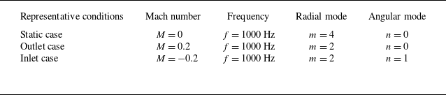
Three different set-ups, each with a single incident mode, are evaluated for validating the proposed model. Detailed information on these cases is shown in table 2. Figure 9 shows the results for sound pressure level (SPL) on different cross-sections. The SPL is defined as
 \begin{equation} \text{SPL} = 20\log _{10}(\overline {p(t)}/p_0), \end{equation}
where
 $\overline {({\cdot })}$
is the time root mean square, and
 $p_0=2\times 10^{-5}\,\textrm {Pa}$
. All SPL results in figure 9 are evaluated at a fixed distance
 $R = 3.5h_0$
from the origin with respect to the corresponding azimuthal angle. The symmetricity of the SPL results can be derived intuitively from the series form of the angular Mathieu functions (see Appendix A). Therefore, the results are plotted on only half the plane. The static, outlet and inlet cases are all assessed for the completeness of this work. Analytical predictions closely match numerical simulations in most assessment positions. It is acknowledged that on the
 $x$
–
 $z$
and
 $y$
–
 $z$
planes, the discrepancy (approximately 3–6 dB) cannot be neglected when
 $\theta _1$
and
 $\theta _2$
are large. These discrepancies are suspected to be instigated by numerical reflections occurring in the FEM computations due to the proximity of the PML to the duct for the sake of reducing computational expenses. As a consequence, the computed solutions will inevitably be slightly contaminated by these numerical reflections, which are usually more eminent at high angles.
Model set-ups for the analytical model and FEM numerical simulation.

The near-field results of instantaneous sound pressure are also compared in figures 10–12, to provide a validation. The computational set-ups are the same as those shown in table 2. Note that the computational domain of the analytical model and the numerical method are not identical: to better conform to the free field boundary conditions, the computational domain used by the FEM numerical simulations is spherical, with a PML in the shape of a spherical shell outside. As a comparison, the computational domain used by the Wiener–Hopf model is an elliptic cylinder, which is naturally generated by the elliptic cylindrical coordinate system. There is no need to add additional absorbent layers since the far-field radiation boundary conditions are already included in the analytical model. To show this difference more clearly, the boundary between the computational domain and the PML in the FEM simulation is marked with dashed lines in figures 10–12.
It is observed that for all three cases, there is a slight discontinuity across the vortex sheet caused by the proposed Wiener–Hopf analytical model. This discrepancy is directly related to the inverse Fourier transform process, as shown in (3.47) and (3.48). Specifically, for
 $\xi \gt \xi _0$
, the third-kind radial Mathieu function and its derivative are used, whereas for
 $\xi \lt \xi _0$
, the first-kind radial Mathieu function and its derivative are used instead. As a result, a discrepancy inevitably arises during the numerical integration process, despite the continuity constraint on pressure. However, this discrepancy can be mitigated by increasing the number of sampling points on the integration path. In this work, the number of sampling points on the integration path
 $\varGamma$
is set to 2048.
Comparison of the SPL results on the
 $(a)$
 $x$
–
 $z$
,
 $(b)$
 $y$
–
 $z$
and
 $(c)$
 $x$
–
 $y$
planes at a constant distance
 $R=3.5h_0$
with respect to the corresponding azimuthal angles
 $\theta _1$
,
 $\theta _2$
and
 $\theta _3$
. The theoretical predictions are denoted by solid lines, and the numerical simulations by dashed lines. The model set-ups correspond to those in table 2 as
 $(\textit{d},\!\textit{e},\!\textit{f})$
static case,
 $(\textit{g},\!\textit{h},\!\textit{i})$
outlet case, and
 $(\kern1.5pt \textit{j},\!\textit{k},\!\textit{l})$
inlet case. The results are evaluated on the
 $(\textit{d},\!\textit{g},\!\textit{j})$
 $x$
–
 $z$
,
 $(\textit{e},\!\textit{h},\!\textit{k})$
 $y$
–
 $z$
and
 $(\kern1.5pt \textit{f},\!\textit{i},\!\textit{l})$
 $x$
–
 $y$
planes. The incident mode has amplitude 1 Pa.

Comparison of the instantaneous sound pressure field from
 $(\textit{a},\!\textit{c})$
theoretical solutions and
 $(\textit{b},\!\textit{d})$
numerical simulations on the
 $(\textit{a},\!\textit{b})$
 $x$
–
 $z$
plane and
 $(\textit{c},\!\textit{d})$
 $y$
–
 $z$
plane, with incident mode
 $(\textit{m},\!\textit{n})=(4,0)$
,
 $f=1000\ \textrm {Hz}$
and
 $M=0$
(the static case). The elliptic duct wall is represented by a thick solid line, and the boundary between the computational domain and the PML in the FEM simulation
 $(\textit{b},\!\textit{d})$
is marked by a thin dashed line. The sound pressure field is shown between
 $\pm 2\ \textrm {Pa}$
using eleven levels.

The model set-up changes to
 $(m,n)=(2,0)$
,
 $f=1000\ \textrm {Hz}$
and
 $M=0.2$
(the outlet case), while the display style remains the same as in figure 10.

The model set-up changes to
 $(m,n)=(2,1)$
,
 $f=1000\ \textrm {Hz}$
and
 $M=-0.2$
(the inlet case), while the display style remains the same as in figure 10.

Figures 13–15 compare the near-field SPL results. Again, only slight discontinuity occurs across the vortex sheet for all analytical results. Overall, the analytical model is in good agreement with the numerical simulations, except for a tendency to slightly overestimate the scattering at large angles outside the duct. As previously stated, this discrepancy can be attributed to the numerical reflections from the PML in the computations.
Comparison of the SPL from
 $(\textit{a},\!\textit{c})$
theoretical solutions and
 $(\textit{b},\!\textit{d})$
numerical simulations on the
 $(\textit{a},\!\textit{b})$
 $x$
–
 $z$
plane and
 $(\textit{c},\!\textit{d})$
 $y$
–
 $z$
plane, with
 $(\textit{m},\textit{n})=(4,0)$
,
 $f=1000\ \textrm {Hz}$
and
 $M=0$
(the static case). The elliptic duct wall is represented by a thick solid line, and the boundary between the computational domain and the PML in the FEM simulation
 $(\textit{b},\!\textit{d})$
is marked by a thin dashed line. The SPL is shown from
 $40\ \textrm {dB}$
to
 $80\ \textrm {dB}$
using nine levels.

The model set-up changes to
 $(m,n)=(2,0)$
,
 $f=1000\ \textrm {Hz}$
and
 $M=0.2$
(the outlet case), while others are the same as those in figure 13.

The model set-up changes to
 $(m,n)=(2,1)$
,
 $f=1000\ \textrm {Hz}$
and
 $M=-0.2$
(the inlet case), while others are the same as those in figure 13.

Parametric study on
 $\xi _0$
to investigate its effect on the far-field directivity in the
 $(a)$
 $x$
–
 $z$
plane,
 $(b)$
 $y$
–
 $z$
plane and
 $(c)$
 $x$
–
 $y$
plane, for incident mode
 $(m,n)=(4,0)$
,
 $f=1000\ \textrm {Hz}$
and
 $M=0$
(the static case).

4.2. Parametric study
A parametric study on
 $\xi _0$
is conducted to examine the effect of the elliptic cross-section shape on the scattered field. As shown in figure 16, the far-field directivity is compared for
 $\xi _0$
values 0.5, 0.6 and 0.8. The corresponding eccentricities of the elliptic cross-section are approximately 0.887, 0.844 and 0.748, respectively.
By comparing figures 16(a) and 16(b), we observe that the SPL on the major-axis plane is higher than that on the minor-axis plane. Moreover, the SPL distribution on the major-axis plane is more uneven: in the forward region of the duct, where the angle
 $\theta _1$
is small, the SPL is significantly higher than in the rear region. As the eccentricity of the elliptic cross-section decreases, the acoustic energy distribution tends to concentrate in the forward direction, on both the major-axis and minor-axis planes. However, this trend manifests differently on each plane: on the major-axis plane, it primarily appears as a decrease in SPL in the rear region, where
 $\theta _1$
is large, while on the minor-axis plane, it is reflected in an increase in SPL in the forward region, where
 $\theta _2$
is small. Overall, as the eccentricity of the elliptic cross-section decreases, the directivity patterns on the major-axis and minor-axis planes become increasingly similar. This aligns with intuition, as a lower eccentricity means that the duct cross-section approaches a circular shape, enhancing its rotational symmetry.
A similar conclusion can be drawn from figure 16(c), which depicts the directivity on the plane coincident with the duct lip and perpendicular to the duct axis. As
 $\xi _0$
increases and the eccentricity of the elliptic cross-section decreases, the SPL distribution along the circumferential direction more closely resembles that of a circular duct, with each wave packet spanning more evenly in the circumferential direction.
4.3. Reflecting modes and analysis
Further analysis is performed here to deepen the understanding of the scattering effect of the duct. To clearly demonstrate the mode scattering back into the elliptic duct and propagating inside the duct along the negative
 $z$
-axis, figure 17 shows the amplitude of the modal spectrum for the reflecting modes. There are two cases evaluated: the static case (
 $M=0$
), with incident mode
 $(m,n) = (4,1)$
, and the inlet case, with incident mode
 $(m,n) = (6,0)$
, both at 2000 Hz.
We find that for an incident mode of even angular order (
 $m\ \text{even}$
), only the modes of even angular order (
 $\tilde {m}\ \text{even}$
) are scattering back into the duct. Under this constraint, nearly all cut-on back-propagating modes occur. And the closer the order is to the incident mode, the more dominant the reflecting mode tends to be.
Reflection modal spectrum of time-harmonic SPL shown with respect to angular and radial elliptic modes. The incident modes are
 $(a)$
 $(m,n)=(4,1)$
,
 $f=2000\ \textrm {Hz}$
,
 $M=0$
, and
 $(b)$
 $(m,n)=(6,0)$
,
 $f=2000\ \textrm {Hz}$
,
 $M=-0.2$
.

4.4. Spinning modes
Spinning modes, also known as rotational acoustic modes, are specific types of wave modes that occur in cylindrical structures, such as tubes and pipes. These modes are characterised by their rotational symmetry, and are particularly relevant in the study of acoustics and vibrations in these structures. Spinning modes can be categorised based on their circumferential (
 $m$
) and radial (
 $n$
) orders, which define their behaviour and propagation characteristics.
The main difference between the rotational acoustic modes in an elliptic duct and those in a circular or annular duct lies in the fact that the axial wavenumbers of the sine and cosine solutions are different. This means that the sine and cosine solutions will experience dispersion as they propagate within the elliptic duct.
In a circular duct with cylindrical coordinates
 $\{r,\theta ,\tilde {z}\}$
, the spinning mode can be expressed as
 \begin{equation} \tilde {P}_{\textit{mn}} = \exp (\textrm {i} m\theta )\,\text{J}_m(\alpha _{\textit{mn}}r) = \cos (m\theta )\,\text{J}_m(\alpha _{\textit{mn}}r)+\textrm {i}\cdot\sin (m\theta )\,\text{J}_m(\alpha _{\textit{mn}}r). \end{equation}
The axial wavenumber
 $k_{\textit{mn}}$
is related to
 $\alpha _{\textit{mn}}$
by (Rienstra & Hirschberg Reference Rienstra and Hirschberg2004)
 \begin{equation} k_{\textit{mn}} = \sqrt {\tilde {\omega }^2-\alpha _{\textit{mn}}^2},\quad \tilde {\omega } = 2\unicode{x03C0} f. \end{equation}
The frequency-domain acoustic field in the circular duct is then given by
 $\tilde {P}_{\textit{mn}}\exp (\textrm {i}k_{\textit{mn}}\tilde {z})$
. Since only one axial wavenumber
 $k_{\textit{mn}}$
is involved, the cosine and sine components of the spinning mode (4.3) propagate in the circular duct at the same speed
 $\tilde {\omega }/k_{\textit{mn}}$
. As a result, their phase angle difference remains constant at
 $90^\circ$
.
Similar to the convention in circular ducts, we use the orthogonality of
 ${\textit{ce}}_m$
and
 ${\textit{se}}_m$
, and construct a complex-valued spinning incident mode as
 \begin{equation} P_{\textit{mn}}(\xi ,\eta ) = {\textit{ce}}_m(\eta ,q_{c,mn})\,{\textit{Mc}}_m^{(1)}(\xi ,q_{c,mn}) + \textrm {i}\cdot {\textit{se}}_m(\eta ,q_{s,mn})\,{\textit{Ms}}_m^{(1)}(\xi ,q_{s,mn}). \end{equation}
Note that generally
 $q_{c,mn} \neq q_{s,mn}$
. By substituting
 $q_{c,mn}$
and
 $q_{s,mn}$
into (2.27), we obtain the axial wavenumbers
 $\mu _{c,mn}^+$
and
 $\mu _{s,mn}^+$
, which are also different. A dispersion would then occur and develop as
 $|z|$
increases if we define the incident wave following the convention
 $\exp (\textrm {i}\omega \mu _{\textit{mn}}^+z)$
.
Dispersion effect is shown by comparing the axial wavenumbers of the elliptic modes of cosine form and sine form. The cosine and sine modes of orders
 $(4,0)$
and
 $(4,1)$
marked within the dashed rectangular box form the corresponding spinning modes in figure 19.

Figure 18 shows the axial wavenumbers for each mode
 $(m,n)$
inside an elliptic duct. We find that the wavenumber of the sine mode is smaller than that of the cosine mode for the same mode
 $(m, n)$
. Furthermore, for the same angular order, the higher the radial order, the more pronounced the dispersion becomes (in terms of both absolute and relative differences in axial wavenumbers). For the same radial order, the higher the angular order, the more pronounced the dispersion becomes (the absolute difference in axial wavenumbers remains relatively constant, while the relative difference increases). For radial order 0, this dispersion is negligible.
Dispersion causes the rotational acoustic modes to deform as
 $|z|$
increases. This effect is more significant inside the duct, as illustrated in figure 19, where figures 19
 $(a)$
and 19
 $(b)$
represent the spinning incident modes
 $(m,n) = (4, 0)$
and
 $(m,n) = (4, 1)$
, respectively. In addition, it can be observed that in figure 19
 $(a)$
, dispersion is negligible, whereas in figure 19
 $(b)$
, the effect of dispersion is significant.
Dispersion causes the rotational acoustic modes to deform as
 $|z|$
increases, for the total spinning sound pressure fields with the incident modes (a)
 $(m,n) = (4, 0)$
and (b)
 $(m,n) = (4, 1)$
. The scattered fields are all calculated using the proposed Wiener–Hopf theoretical approach.

5. Conclusion
In this paper, we develop an analytical model based on the Wiener–Hopf technique to solve the problem of acoustic field scattering from a semi-infinite elliptic duct with uniform subsonic flow. We introduce the elliptic cylindrical coordinate system as a suitable mathematical tool for addressing wave equations with elliptic boundary conditions. The well-known Mathieu functions are employed to constitute general solutions both inside and outside the duct. For waves propagating inside the duct, radial Mathieu functions of the first kind are used to express the radial distribution. For the acoustic field outside the duct, radial Mathieu functions of the third kind are necessary to describe the radiation of waves to infinity. The Fourier transform along the axial direction is utilised to convert the mixed boundary condition from the physical model into a Wiener–Hopf equation. A series decomposition method using angular Mathieu functions as the basis is implemented to transform the original three-dimensional problem into a set of Wiener-Hopf equations with scalar kernel functions. The classical kernel factorisation method is then used to solve the Wiener–Hopf equations.
The core of our research lies in emulating the Fourier series by employing angular Mathieu functions as basis functions (McLachlan Reference McLachlan1947). The incident acoustic field on the vortex sheet, along with the unknown functions induced by it, is expanded into a series along the azimuthal direction. This approach reformulates the problem into the solution of a set of Wiener–Hopf equations, from which the coefficients of the series expansion are determined.
For validation, the solution obtained by the proposed analytical model is compared with numerical FEM simulation results, showing sufficient consistency. The model is further used to calculate the reflection coefficients, revealing that the reflected elliptic modes with angular and radial mode numbers similar to those of the incident mode are dominant when reflecting back into the duct. Moreover, when adopting an elliptic incident mode of even form, only modes of even form reflect back.
Finally, we consider a critical application of this theoretical model: the inlet of aeroengines with a spinning mode as the incident mode. We construct a spinning elliptic mode imitating the circular mode by setting the elliptic mode of cosine form as the real part, and the sine form as the imaginary part. Unlike the circular mode, these two parts of an elliptic mode typically have different axial wavenumbers, causing dispersion when propagating inside the duct.
The innovative aspect of this theoretical development lies in its extension of the Wiener–Hopf method’s capabilities to analyse sound propagation in elliptic-shaped duct configurations, beyond traditional cylindrical duct set-ups. The incorporation of Mathieu functions into the Wiener–Hopf model offers a versatile and generic approach that could be applicable to various new problems, including lining elliptic-shaped ducts and investigating elliptic outlets in shear flows. This theoretical model is expected to contribute substantially to deepening our understanding of wave mechanics within elliptic-shaped ducts, and offers a foundation for the design and optimisation of future low-noise aircraft.
Funding
This work is supported by the National Science Foundation of China (12432016, 12272007) and the Technical Field Fund of Foundation Strengthening Programme (2021-JCJQ-JJ-0017).
Declaration of interests
The authors report no conflict of interest.
Appendix A. Calculation of Mathieu functions
Following Olver et al. (Reference Olver, Lozier, Boisvert and Clark2010), angular Mathieu functions are expressed as the Fourier series
 \begin{align} {\textit{ce}}_{2m}(z,q) &= \sum _{l = 0}^{\infty } A_{2l}^{2m}(q)\cos 2lz, \end{align}
 \begin{align} {\textit{ce}}_{2m+1}(z,q) &= \sum _{l = 0}^{\infty } A_{2l+1}^{2m+1}(q)\cos (2l+1)z, \end{align}
 \begin{align} {\textit{se}}_{2m+1}(z,q) &= \sum _{l = 0}^{\infty } B_{2l+1}^{2m+1}(q)\sin (2l+1)z, \end{align}
 \begin{align} {\textit{se}}_{2m+2}(z,q) &= \sum _{l = 0}^{\infty } B_{2l+2}^{2m+2}(q)\sin (2l+2)z, \end{align}
where the coefficients are obtained from the following recurrence relations:
 \begin{align} -aA_0 + qA_2 &= 0, \nonumber \\ 2qA_0 + (4-a)A_2 + qA_4 &= 0, \nonumber \\ qA_{2l-2} + [(2l)^2-a]A_{2l} + qA_{2l+2} &= 0,\nonumber \\ l = 2,3,4,\ldots , & \quad a = a_{2m}(q), \quad A_{2l} = A_{2l}^{2m}, \end{align}
 \begin{align} (1+q-a)A_1 + qA_3 &= 0,\nonumber \\ qA_{2l-1} + [(2l+1)^2-a]A_{2l+1} + qA_{2l+3} &= 0, \nonumber \\ l = 1,2,3,\ldots , &\quad a = a_{2m+1}(q), \quad A_{2l+1} = A_{2l+1}^{2m+1}, \end{align}
 \begin{align} (1+q-b)B_1 + qB_3 &= 0,\nonumber \\ qB_{2l-1} + [(2l+1)^2-b]B_{2l+1} + qB_{2l+3} &= 0,\nonumber \\ l = 1,2,3,\ldots , &\quad b = b_{2m+1}(q), \quad B_{2l+1} = B_{2l+1}^{2m+1}, \end{align}
 \begin{align} (4-b)B_2 + qB_4 &= 0, \nonumber \\ qB_{2l-2} + [(2l)^2-b]B_{2l} + qB_{2l+2} &= 0,\nonumber \\ l = 2,3,4,\ldots , &\quad b = b_{2m+2}(q), \quad B_{2l+2} = B_{2l+2}^{2m+2}. \end{align}
Each set of recurrence relations (A5)–(A8) can be solved by addressing the corresponding eigenvalue problem, where
 $a_{2m}(q)$
,
 $a_{2m+1}(q)$
,
 $b_{2m+1}(q)$
and
 $b_{2m+2}(q)$
are eigenvalues, and
 $A_{2l}^{2m}$
,
 $A_{2l+1}^{2m+1}$
,
 $B_{2l+1}^{2m+1}$
and
 $B_{2l+2}^{2m+2}$
are eigenvectors. Eigenvectors require careful sorting and normalisation, especially when the parameter
 $q$
is complex (Ziener et al. Reference Ziener, Rückl, Kampf, Bauer and Schlemmer2012).
Radial Mathieu functions can be calculated in the series of cross-products of Bessel functions as
 \begin{align} {\textit{Mc}}_{2m}^{(j)}(z,h) &= \sum _{l=0}^{\infty }(-1)^{m+l}\frac {A_{2l}^{2m}(h^2)}{A_{0}^{2m}(h^2)}\big [ \text{J}_l(he^{-z})\,\textrm {F}_l^{(j)}(he^{z}) \big ], \end{align}
 \begin{align} {\textit{Mc}}_{2m+1}^{(j)}(z,h) &= \sum _{l=0}^{\infty }(-1)^{m+l}\frac {A_{2l+1}^{2m+1}(h^2)}{A_{1}^{2m+1}(h^2)}\big [\text{J}_l(he^{-z})\,\textrm {F}_{l+1}^{(j)}(he^{z}) +\text{J}_{l+1}(he^{-z})\,\textrm {F}_{l}^{(j)}(he^{z}) \big ], \end{align}
 \begin{align} {\textit{Ms}}_{2m+1}^{(j)}(z,h) &= \sum _{l=0}^{\infty }(-1)^{m+l}\frac {B_{2l+1}^{2m+1}(h^2)}{B_{1}^{2m+1}(h^2)}\big [ \text{J}_l(he^{-z})\,\textrm {F}_{l+1}^{(j)}(he^{z}) +\text{J}_{l+1}(he^{-z})\,\textrm {F}_{l}^{(j)}(he^{z}) \big ], \end{align}
 \begin{align} {\textit{Ms}}_{2m+2}^{(j)}(z,h) &= \sum _{l=0}^{\infty }(-1)^{m+l}\frac {B_{2l+2}^{2m+2}(h^2)}{B_{2}^{2m+2}(h^2)}\big [ \text{J}_l(he^{-z})\,\textrm {F}_{l+2}^{(j)}(he^{z}) +\text{J}_{l+2}(he^{-z})\,\textrm {F}_{l}^{(j)}(he^{z}) \big ], \end{align}
where
 $h = q^{1/2}$
,
 $j=1,2,3,4$
and
 $\textrm {F}_{l}^{(j)}$
denotes Bessel functions of the first kind
 $\text{J}_l$
, Neumann function
 $\textrm {N}_l$
, Hankel function of the first kind
 $\textrm {H}_{l}^{(1)}$
, and Hankel function of the second kind
 $\textrm {H}_{l}^{(2)}$
when
 $j = 1$
,
 $j = 2$
,
 $j = 3$
and
 $j = 4$
, respectively.
Appendix B. Decomposition of
 $\boldsymbol{G}_{\boldsymbol{+}}$
in the series of angular Mathieu functions

The decomposition of
 $G_+(\eta ,u)$
needs to introduce a discretisation, in which
 $G_+(\eta ,u)$
is described over an
 $I\times 1$
mesh along the angular direction, where
 $I$
represents the number of mesh points. This discretisation indicates
 \begin{equation} \boldsymbol{G}_+(u) = \left [ \begin{array}{c} G_+(\eta _1,u) \\[3pt] G_+(\eta _2,u) \\ \vdots \\ G_+(\eta _i,u) \\ \vdots \\ G_+(\eta _I,u) \end{array} \right ]\!. \end{equation}
The transfer function from the decomposed
 $\hat {G}_{+,\kappa }(u)$
to the discretised
 $\boldsymbol{G}_+(u)$
can then be written as
 \begin{equation} \unicode{x1D64F}\hat {G}_{+,\kappa }(u) = \boldsymbol{G}_+(u), \end{equation}
where
 $\hat {G}_{+,\kappa }(u)$
is the truncation with a finite number
 $T_N$
, i.e.
 \begin{equation} \hat {G}_{+,\kappa }(u) = \left [ \begin{array}{c} \hat {G}_{+,0}(u) \\[3pt] \hat {G}_{+,1}(u) \\ \vdots \\ \hat {G}_{+,\kappa }(u) \\ \vdots \\ \hat {G}_{+,T_N}(u) \end{array} \right ]\!, \end{equation}
and
 $\unicode{x1D64F}$
is the
 $I\times (T_N+1)$
transfer matrix
 \begin{equation} \unicode{x1D64F} = \left [ \begin{array}{cccccc} {\textit{ce}}_0(\eta _1,Q) & {\textit{ce}}_1(\eta _1,Q) & {\cdots} & {\textit{ce}}_\kappa (\eta _1,Q) & {\cdots} & {\textit{ce}}_{T_N}(\eta _1,Q) \\[3pt] {\textit{ce}}_0(\eta _2,Q) & {\textit{ce}}_1(\eta _2,Q) & {\cdots} & {\textit{ce}}_\kappa (\eta _2,Q) & {\cdots} & {\textit{ce}}_{T_N}(\eta _2,Q) \\ \vdots & \vdots & \ddots & \vdots & \ddots & \vdots \\ {\textit{ce}}_0(\eta _i,Q) & {\textit{ce}}_1(\eta _i,Q) & {\cdots} & {\textit{ce}}_\kappa (\eta _i,Q) & {\cdots} & {\textit{ce}}_{T_N}(\eta _i,Q) \\ \vdots & \vdots & \ddots & \vdots & \ddots & \vdots \\ {\textit{ce}}_0(\eta _I,Q) & {\textit{ce}}_1(\eta _I,Q) & {\cdots} & {\textit{ce}}_\kappa (\eta _I,Q) & {\cdots} & {\textit{ce}}_{T_N}(\eta _I,Q) \end{array} \right ]\!. \end{equation}
The row number of
 $\unicode{x1D64F}$
is much larger than its column number (
 $I\gg T_N+1$
). Since
 $\unicode{x1D64F}$
and
 $\boldsymbol{G}_+(u)$
are already known, we can simply use the Moore–Penrose pseudo-inverse (see Ben-Israel & Greville Reference Ben-Israel and Greville2003), denoted as
 $\text{pinv}({\cdot })$
, to solve (B2) as
 \begin{equation} \hat {G}_{+,\kappa }(u) = \text{pinv}(\unicode{x1D64F}\,)\,\boldsymbol{G}_+(u). \end{equation}
Convergence tests were conducted to ensure the accuracy of this decomposition method.