1 Introduction
Nonlinear partial differential equations (PDEs) serve as powerful tools for describing intricate real-world phenomena in engineering and scientific disciplines. Fisher and Burgers–Fisher (BF) equations exemplify such PDEs [Reference Fisher17], playing a crucial role in diverse applications. These equations find relevance in biological and chemical processes, including gene propagation [Reference Fisher17], as well as in engineering domains such as combustion [Reference Aggarwal2], tissue engineering [Reference Maini, McElwain and Leavesley27], neurophysiology [Reference Tuckwell43] and autocatalytic chemical reactions [Reference Aronson and Weinberger4]. Furthermore, the Fisher equation extends its applicability to population dynamics, encompassing scenarios involving cells in tumours, human populations or even fish populations. The BF equation emerged as a fusion of two renowned equations: the Burgers equation, derived from the works of Burgers [Reference Burgers11] and Bateman [Reference Bateman8], and the Fisher equation, pioneered by Fisher [Reference Fisher17]. This amalgamation of these influential equations has given rise to a powerful mathematical model that captures the essence of both disciplines. The one-dimensional nonlinear BF equation is given as
 $$ \begin{align} \frac{\partial u}{\partial t}+\alpha u \frac{\partial u}{\partial x}=\varepsilon \frac{\partial^2 u}{\partial x^2}+\beta u(1-u),\quad x\in(a_1,a_2),\ t\geq0, \end{align} $$
with initial condition
 $$ \begin{align} u(x,0)=f_0(x), \quad x\in(a_1,a_2), \end{align} $$
and boundary conditions
 $$ \begin{align} u(a_1,t)=f_1(t),\quad u(a_2,t)=f_2(t),\ t\in[0,T], \end{align} $$
where
 $\alpha $
,
 $\beta $
are real numbers and
 $0\leq \varepsilon \leq 1$
. It is known as the Burgers–Fisher (BF) equation, because it has convective phenomena from Burger’s equation and diffusion transport along with reaction characteristics from Fisher’s equation. This equation is highly nonlinear, because of the presence of convection, diffusion and reaction mechanisms. With
 $\alpha = 0$
, equation (1.1) reduces to the Fisher equation, which was used by Murray [Reference Murray33] in mathematical biology. Ablowitz and Zeppetella [Reference Ablowitz and Zeppetella1] presented explicit solutions of the Fisher equation. For
 $\beta =0$
, the given equation is known as the Burgers equation. Sachdev [Reference Sachdev37] used self-similarity for the exact solution of the BF equation.
Due to their vast and far-reaching applications across the fields of applied sciences and engineering, the abovementioned equation (1.1) has garnered immense popularity and significance among researchers, making it the subject of intense study and analysis. Several analytical and numerical methods are given by researchers for Fisher and BF equations. Kaya and Sayed [Reference Kaya and El-Sayed22] used the Adomian decomposition method without any discretization for the numerical solution of the generalized Burgers–Fisher (gBF) equation and obtained an exact solution in the form of a series without any classical transformation. Javidi [Reference Javidi21] developed a spectral collocation method, which is a combination of the pseudospectral Chebyshev method and Runge–Kutta fourth-order method for the numerical study of the gBF. A variational iteration scheme was applied by Moghimi and Hejazi [Reference Moghimi and Hejazi32], in which Lagrange multipliers were used to construct correction functions for the gBF. Zhu and Kang [Reference Zhu and Kang48] used the cubic B-spline quasi-interpolation technique to solve the BF equation. A modified cubic B-spline collocation method with the strong stability preserving RK-54 scheme was used by Mittal and Tripathi [Reference Mittal and Tripathi31] for the numerical solution of the gBF equation. Sangwan and Kaur [Reference Sangwan and Kaur39] applied a finite element approach, in which the implicit Euler method is used for time discretization, exponentially fitted splines for space discretization and piecewise uniform Shishkin mesh is used for the spatial domain.
Balyan et al. [Reference Balyan, Mittal, Kumar and Choube7] proposed the pseudospectral method for this equation. The method used the Chebyshev–Gauss–Lobatto points and applied collocation methods in space and time. This allows the study of travelling wave solutions that transform into shock-like wavefronts and then change shape into complex wave patterns. Arora et al. [Reference Arora, Jain and Kukreja5] applied the robust Hermite collocation technique to solve different kinds of Burgers equations. This technique employs the Hermite collocation method, using fifth-order Hermite splines to approximate the solution variable and its spatial derivatives. For the time derivatives, the Crank–Nicholson finite difference scheme is applied, ensuring a robust and accurate numerical solution. A hybrid scheme has been implemented by Akinfe and Loyinmi [Reference Akinfe and Loyinmi3] to solve the gBF equation. This approach involves the coupling of the new Elzaki integral transform, an improved version of the renowned Laplace transform, with a modified differential transform technique called the projected differential transform method.
A combined spectral matrix collocation strategy has been proposed by Izadi and Srivastava [Reference Izadi and Srivastava20] for this equation. For every time step, the linear initial boundary value problem is addressed using a spectral collocation technique that employs novel Boole polynomials as the basis functions. Tantawy et al. [Reference El-Tantawy, Matoog, Shah, Alrowaily and Ismaeel16] used the residual power series transform method (combines two algorithms: the Laplace transform and the residual power series method) for solving the given equation. Various other methods have been proposed like the exponential time differencing technique with the method of lines [Reference Bratsos and Khaliq10], a modified cubic B-spline collocation method [Reference Mittal and Jain29], an extended modified cubic B-spline algorithm [Reference Shuklav and Tamsir41], the pseudospectral method [Reference Olmos and Shizgal34], the exponential cubic B-spline method [Reference Dag and Ersoy14], the wavelet Galerkin method [Reference Mittal and Kumar30], the moving mesh method [Reference Qiu and Sloan35], the Galerkin method [Reference Dag, Sahin and Korkmaz15], the quintic B-splines collocation method [Reference Sahin and Ozmen38], the sinc collocation method [Reference Khaled23] and the implicit numerical technique [Reference Chandraker and Awasthi13] for this equation.
In this paper, the hepta Hermite collocation method (HHCM) has been used to solve both Fisher and Burgers–Fisher equations. It is an orthogonal collocation method in which hepta Hermite interpolating polynomials have been used as a basis function. The hepta Hermites have continuity of the dependent variable and its first three derivatives throughout the solution range. Using the Hermite function in the collocation method leads to banded matrices. The Crank–Nicholson scheme for temporal domain and hepta Hermite is applied to discretize the space domain. The combination of a Crank–Nicholson scheme and a hepta Hermite collocation scheme provides better accuracy and simplicity with better numerical stability than other methods given in the literature. The hepta Hermite collocation technique is found to be quite easy, accurate and reliable.
The paper is arranged as follows. In Section 2, the hepta Hermite collocation method is discussed. Implementation of the proposed method on Fisher and Burgers–Fisher equations is discussed in Section 3. The stability analysis of the HHCM is discussed in Section 4. In Section 5, error bounds estimates of hepta Hermite interpolation and convergence analysis are presented. In Section 6, a few examples are given to show the efficiency of the HHCM. The conclusion is given in Section 7.
2 Hepta Hermite collocation method
In the hepta Hermite collocation method (HHCM), the space domain
 $[a_1,a_2]$
is divided, that is,
 $a_1 = x_{1} < x_{2} < \cdots < x_{N} < x_{N+1} = a_2$
, into N number of subdomains, called finite element with uniform step size h, where
 $x_{k+1}=x_k+h$
for
 $k=1,2,\ldots ,N+1$
and
 $h=(a_2-a_1)/N$
. The HHCM is a generalization of the orthogonal collocation method on finite element using hepta Hermite interpolating polynomials as a basis function, which interpolates the approximate function as well as its first three derivatives at each node point. In HHCM, the approximate function is written as a linear combination of Hermite polynomials with degree seven as follows:
 $$ \begin{align*} u(x,t)=\sum_{k=1}^{N+1}[a_k(t)p_k(x)+b_k(t)q_k(x)+c_k(t)r_k(x)+d_k(t)s_k(x)], \end{align*} $$
where
 $a_k(t),~b_k(t),~c_k(t)$
and
 $d_k(t)$
are continuous functions of t, and
 $p_k,~q_k,~r_k$
,
 $s_k$
are Hermite basis functions of degree seven given by
 $$ \begin{align*} &p_{k}(x)=\\ &\quad\begin{cases} \displaystyle 35\bigg(\frac{x-x_{k-1}}{h}\bigg)^{4}-84\bigg(\frac{x-x_{k-1}}{h}\bigg)^{5}+70\bigg(\frac{x-x_{k-1}}{h}\bigg)^{6}-20\bigg(\frac{x-x_{k-1}}{h}\bigg)^{7}, &x\in[x_{k-1},x_{k}], \\[6pt] \displaystyle 35\bigg(\frac{x_{k+1}-x}{h}\bigg)^{4}-84\bigg(\frac{x_{k+1}-x}{h}\bigg)^{5}+70\bigg(\frac{x_{k+1}-x}{h}\bigg)^{6}-20\bigg(\frac{x_{k+1}-x}{h}\bigg)^{7}, &x\in[x_{k},x_{k+1}],\\ 0, &\text{otherwise}, \end{cases} \end{align*} $$
 $$ \begin{align*} &q_{k}(x)=\\ &\quad\begin{cases} \displaystyle -15\frac{(x-x_{k-1})^{4}}{h^{3}}+39\frac{(x-x_{k-1})^{5}}{h^{4}}-34\frac{(x-x_{k-1})^{6}}{h^{5}}+10\frac{(x-x_{k-1})^{7}}{h^{6}}, &x\in[x_{k-1},x_{k}], \\[6pt] \displaystyle -15\frac{(x_{k+1}-x)^{4}}{h^{3}}+39\frac{(x_{k+1}-x)^{5}}{h^{4}}-34\frac{(x_{k+1}-x)^{6}}{h^{5}}+10\frac{(x_{k+1}-x)^{7}}{h^{6}}, &x\in[x_{k},x_{k+1}],\\ 0, &\text{otherwise}, \end{cases} \end{align*} $$
 $$ \begin{align*} &r_{k}(x)=\\ &\quad\begin{cases} \displaystyle \frac{5}{2}\frac{(x-x_{k-1})^{4}}{h^{2}}-7\frac{(x-x_{k-1})^{5}}{h^{3}}+\frac{13}{2}\frac{(x-x_{k-1})^{6}}{h^{4}}-2\frac{(x-x_{k-1})^{7}}{h^{5}}, &x\in[x_{k-1},x_{k}], \\[6pt] \displaystyle\frac{5}{2}\frac{(x_{k+1}-x)^{4}}{h^{2}}-7\frac{(x_{k+1}-x)^{5}}{h^{3}}+\frac{13}{2}\frac{(x_{k+1}-x)^{6}}{h^{4}}-2\frac{(x_{k+1}-x)^{7}}{h^{5}}, &x\in[x_{k},x_{k+1}],\\ 0, &\text{otherwise}, \end{cases} \end{align*} $$
 $$ \begin{align*} &s_{k}(x)=\\ &\quad\begin{cases} \displaystyle-\frac{1}{6}\frac{(x-x_{k-1})^{4}}{h}+\frac{1}{2}\frac{(x-x_{k-1})^{5}}{h^{2}}-\frac{1}{2}\frac{(x-x_{k-1})^{6}}{h^{3}}+\frac{1}{6}\frac{(x-x_{k-1})^{7}}{h^{4}}, &x\in[x_{k-1},x_{k}], \\[6pt] \displaystyle-\frac{1}{6}\frac{(x_{k+1}-x)^{4}}{h}+\frac{1}{2}\frac{(x_{k+1}-x)^{5}}{h^{2}}-\frac{1}{2}\frac{(x_{k+1}-x)^{6}}{h^{3}}+\frac{1}{6}\frac{(x_{k+1}-x)^{7}}{h^{4}}, &x\in[x_{k},x_{k+1}],\\ 0, &\text{otherwise}, \end{cases} \end{align*} $$
with
 $p_{k}(x_i)=1$
,
 $q^{\prime }_{k}(x_i)=1$
,
 $r^{\prime \prime }_{k}(x_i)=1$
,
 $s^{\prime \prime \prime }_{k}(x_i)=1$
when
 $k=i$
,
 $k=1,2,\ldots ,N+1$
and
 $i=1,2,\ldots ,N+1$
. Other values, that is,
 $k\neq i$
, of hepta Hermite interpolating polynomials and their first, second and third derivatives vanish at the remaining points. For more detail, we refer the reader to [Reference Kumari and Kukreja26]. After the discretization of the domain, each element
 $[x_{r},x_{r+1}]$
is mapped on to
 $[0,1]$
by using the following transformation:
 $$ \begin{align} \chi=\frac{x-x_{r}}{h}, \quad r=1,2,\ldots,N, \end{align} $$
where
 $h=x_{r+1}-x_r$
,
 $\chi =0$
at
 $x=x_r$
and
 $\chi =1$
at
 $x=x_{r+1}$
. In HHCM, six interior collocation points within each element
 $[x_{r},x_{r+1}]$
are introduced. These collocation points are the roots of six degree shifted Legendre polynomials [Reference Kumari and Kukreja24]. The orthogonal collocation method with a hepta Hermite basis function is applied on
 $\chi $
within each element. By using equation (2.1) and rearranging the terms, the hepta Hermite interpolating functions
 $p_k, q_k, r_k$
and
 $s_k$
in terms of
 $\chi $
, that is,
 $H_{1}(\chi ), H_{2}(\chi ),\ldots ,H_{8}(\chi )$
, are given in [Reference Kumari and Kukreja25], with
 $ H_{1}(\chi )=H_{8}(1-\chi )$
,
 $ H_{2}(\chi )=-H_{7}(1-\chi )$
,
 $ H_{3}(\chi )=H_{6}(1-\chi )$
and
 $ H_{4}(\chi )=-H_{5}(1-\chi )$
. A graphical representation of hepta Hermite is given in [Reference Kumari and Kukreja24]. After using equation (2.1) and re-arranging the terms, the trial function in the rth element can be written as
 $$ \begin{align} U(\chi,t)=\sum_{i=1}^{8} a_{i+6r-6}(t)H_{i}(\chi_j),\quad 0\leq\chi\leq1, \end{align} $$
where
 $a_{i+6r-6}(t)$
are the time dependent unknown quantities to be determined.
3 Implementation of proposed technique
Let
 $0 = t_{0} < t_{1} <\cdots < t_{n} < t_{n+1}<\cdots \leq T$
be the partition of time domain
 $[0,T]$
with step size
 $\Delta t$
, where
 $t_{n+1} = t_{n} + \Delta t$
, for
 $n=0, 1,\ldots , m$
. Applying the Crank–Nicholson scheme to discretize equations (1.1)–(1.3),
 $$ \begin{align} &\frac{u^{n+1}-u^{n}}{\Delta t} + \alpha \bigg[ \frac{(u u_{x})^{n+1} + (u u_{x})^{n}}{2}\bigg]\nonumber\\ &\quad= \varepsilon \bigg[\frac{u_{xx}^{n+1} + u_{xx}^{n}}{2} \bigg] +\beta\bigg[ \frac{u^{n+1} + u^{n}}{2}\bigg] - \beta \bigg[ \frac{(u^2)^{n+1} + (u^2)^{n}}{2}\bigg]. \end{align} $$
Using the quasilinearization process [Reference Kumari and Kukreja25] to linearize the nonlinear terms in equation (3.1), we get
 $$ \begin{align*} \begin{aligned} (u^2)^{n+1}+(u^2)^{n} &= 2u^n u^{n+1} + O(\Delta t ^{2}),\\ (uu_{x})^{n+1}+(uu_{x})^{n}& = u^n u_x^{n+1}+u^{n+1} u_x^{n} + O(\Delta t ^{2}). \end{aligned} \end{align*} $$
Using the above values in equation (3.1) and separating the
 $n$
th and
 $(n+1)$
th level terms, we have
 $$ \begin{align} u^{n+1}+\frac{\Delta t}{2}[\alpha(u^{n}u_{x}^{n+1}+u^{n+1}u_{x}^{n})-\varepsilon u_{xx}^{n+1}-\beta(u^{n+1}-2u^n u^{n+1}) ] = u^{n}+\frac{\Delta t}{2}[\varepsilon u_{xx}^{n}+\beta u^{n}]. \end{align} $$
After substituting equation (2.2), at the jth collocation point, equation (3.2) can be rewritten as
 $$ \begin{align} &\sum_{i=1}^{8}a^{n+1}_{i+6r-6}\bigg[H_i(\chi_j)+\frac{\Delta t}{2}\bigg(\frac{\alpha}{h}(u^{n}H^{\prime}_i(\chi_j)+u_x^{n}H_i(\chi_j))-\frac{\varepsilon }{h^2} H^{\prime\prime}_i(\chi_j) -\beta(H_i(\chi_j)-2u^n H_i(\chi_j))\bigg)\bigg] \notag \\ &\quad=\sum_{i=1}^{8}a^{n}_{i+6r-6}\bigg[H_i(\chi_j)+\frac{\Delta t}{2}\bigg(\frac{\varepsilon }{h^2} H^{\prime\prime}_i(\chi_j)+\beta H_i(\chi_j)\bigg) \bigg] \end{align} $$
and
 $$ \begin{align} \begin{aligned} &u(\chi_jh+x_r,0)=f_0(\chi_jh+x_r),\\ &u(a_1,t_n)=f_1(t_n),\quad u(a_2,t_n)=f_2(t_n),\quad n=0,1,\ldots,m, \end{aligned} \end{align} $$
with
 $r=1,2,\ldots ,N$
and
 $j=1,2,\ldots ,6$
.
From equation (3.3), a system of
 $6N$
equations in
 $(6N+2)$
unknowns is formed. The remaining two unknowns are calculated from equation (3.4). Therefore, the system of equations can be written as
 $$ \begin{align} HA=D, \quad \text{where}\end{align} $$

 $$ \begin{align*}A= \left[\begin{array}{ccccccccc} a^{n+1}_{1}\\ a^{n+1}_{2}\\ a^{n+1}_{3}\\ a^{n+1}_{4}\\ a^{n+1}_{5}\\ a^{n+1}_{6}\\ a^{n+1}_{7}\\ a^{n+1}_{8}\\ a^{n+1}_{9}\\ a^{n+1}_{10}\\ a^{n+1}_{11}\\ a^{n+1}_{12}\\ .\\ .\\ a^{n+1}_{6N-5}\\ a^{n+1}_{6N-4}\\ a^{n+1}_{6N-3}\\ a^{n+1}_{6N-2}\\ a^{n+1}_{6N-1}\\ a^{n+1}_{6N}\\ a^{n+1}_{6N+1}\\ a^{n+1}_{6N+2}\\ \end{array} \right],\quad D = \left[\begin{array}{ccccccccc} f_{1}(n \Delta t)\\ \delta_1^1\\ \delta_2^1\\ \delta_3^1\\ \delta_4^1\\ \delta_5^1\\ \delta_6^1\\ \delta_1^2\\ \delta_2^2\\ \delta_3^2\\ \delta_4^2\\ \delta_5^2\\ \delta_6^2\\ .\\ .\\ \delta_1^N\\ \delta_2^N\\ \delta_3^N\\ \delta_4^N\\ \delta_5^N\\ f_{2}(n \Delta t)\\ \delta_6^N\\ \end{array} \right] \end{align*} $$
with
 $$ \begin{align*} \xi_{ji}^{r}&=\bigg[H_i(\chi_j)+\frac{\Delta t}{2}\bigg(\frac{\alpha}{h}(u^{n}H^{\prime}_i(\chi_j)+u_x^{n}H_i(\chi_j))-\frac{\varepsilon }{h^2}H^{\prime\prime}_i(\chi) -\beta(H_i(\chi_j)-2u^n H_i(\chi_j))\bigg)\bigg],\\ \delta_{j}^{r}&=\sum_{i=1}^{8}a^{n}_{i+6r-6}\bigg[H_i(\chi_j)+\frac{\Delta t}{2}\bigg(\frac{\varepsilon }{h^2}H^{\prime\prime}_i(\chi)+\beta H_i(\chi_j)\bigg) \bigg], \end{align*} $$
for
 $j=1,2,\ldots ,6$
,
 $i=1,2,\ldots ,8$
,
 $n=0,1,\ldots ,m$
and
 $r=1,2,\ldots ,N$
, H is a
 $(6N+2) \times (6N+2)$
matrix, A and D are
 $(6N+2) \times 1$
column vectors. The matrix H is diagonally dominant. The value of
 $A^0=[a_{1}^{0},a_{2}^{0},\ldots ,a_{6N+2}^{0}]$
is required to find the solution at the next time level. The unknown
 $A^0$
is calculated from the initial condition in equation (3.4) as given below:

 $$ \begin{align*} \times \left[\begin{array}{ccccccccc} a^{0}_{1}\\ a^{0}_{2}\\ a^{0}_{3}\\ a^{0}_{4}\\ a^{0}_{5}\\ a^{0}_{6}\\ a^{0}_{7}\\ a^{0}_{8}\\ a^{0}_{9}\\ a^{0}_{10}\\ a^{0}_{11}\\ a^{0}_{12}\\ .\\ .\\ a^{0}_{6N-5}\\ a^{0}_{6N-4}\\ a^{0}_{6N-3}\\ a^{0}_{6N-2}\\ a^{0}_{6N-1}\\ a^{0}_{6N}\\ a^{0}_{6N+1}\\ a^{0}_{6N+2}\\ \end{array} \right] = \left[\begin{array}{ccccccccc} f_{0}(a_1)\\ f_{01}^1\\ f_{02}^1\\ f_{03}^1\\ f_{04}^1\\ f_{05}^1\\ f_{06}^1\\ f_{01}^2\\ f_{02}^2\\ f_{03}^2\\ f_{04}^2\\ f_{05}^2\\ f_{06}^2\\ .\\ .\\ f_{01}^N\\ f_{02}^N\\ f_{03}^N\\ f_{04}^N\\ f_{05}^N\\ f_{0}(a_2)\\ f_{06}^N\\ \end{array} \right] \end{align*} $$
where
 $H_{ji}^r=H_i(\chi _j)$
,
 $f_{0j}^r=f_0(\chi _jh+x_r)$
. The above system is solved using MATLAB 2022.
4 Stability analysis
The von Neumann method is applied for stability analysis of the proposed hepta Hermite collocation method. For this, take u as a local constant w to linearize the nonlinear terms and further discretize the temporal domain using the Crank–Nicholson scheme, then we get
 $$ \begin{align*} \frac{u^{n+1} - u^{n}}{\Delta t} + \alpha w \bigg[\frac{(u_{x})^{n+1} + (u_{x})^{n}}{2}\bigg]= \varepsilon \frac{(u_{xx})^{n+1} + (u_{xx})^{n}}{2} + \beta (1 - w)\bigg[\frac{u^{n+1} + u^{n}}{2} \bigg]. \end{align*} $$
Separate the
 $(n+1)$
th and nth time level terms:
 $$ \begin{align*} \frac{u^{n+1}}{\Delta t}+\frac{\alpha w}{2}(u_{x})^{n+1}-\frac{\varepsilon}{2}u_{xx}^{n+1}-\frac{\beta(1 - w)}{2}u^{n+1} =\frac{u^{n}}{\Delta t}-\frac{\alpha w}{2}(u_{x})^{n}+\frac{\varepsilon}{2}u_{xx}^{n}+\frac{\beta(1 - w)}{2}u^{n}. \end{align*} $$
After using HHCM, the above equation can be written as
 $$ \begin{align*} &\sum_{i=1}^{8} a_{i+6r-6}^{n+1}\bigg[\frac{H_i(\chi_j)}{\Delta t}+\frac{\alpha w}{2h}H^{\prime}_i(\chi_j)-\frac{\varepsilon}{2h^2}H^{\prime\prime}_i(\chi_j)-\frac{\beta (1 - w)}{2}H_i(\chi_j)\bigg]\\ &\quad =\sum_{i=1}^{8} a_{i+6r-6}^{n}\bigg[\frac{H_i(\chi_j)}{\Delta t}-\frac{\alpha w}{2h}H^{\prime}_i(\chi_j)+\frac{\varepsilon}{2h^2}H^{\prime\prime}_i(\chi_j)+\frac{\beta (1 - w)}{2}H_i(\chi_j)\bigg]. \end{align*} $$
Putting
 $a_{i}^{n} = W \gamma ^{n} e^{(i\iota \phi h)}$
, where W is the amplitude,
 $\iota = \sqrt {-1}$
, h is the space step length and
 $\phi $
is the mode number, we get
 $$ \begin{align} &\gamma^{n+1}\bigg[\sum_{i=1}^{8}\exp((i+6e-6)h\phi \iota)\sigma_i\bigg]=\gamma^{n}\bigg[\sum_{i=1}^{8}\exp((i+6e-6)h\phi \iota)\rho_i\bigg]\\ &\quad\implies\kern-2pt \gamma^{n+1}\sum_{i=1}^{8}[\cos((i+6e-6)h\phi)+\iota\sin((i+6e-6)h\phi) ]\sigma_i \notag \\ &\quad=\gamma^{n}\sum_{i=1}^{8}[\cos((i+6e-6)h\phi)+\iota\sin((i+6e-6)h\phi)]\rho_i, \notag \end{align} $$
where
 $$ \begin{align*} &\sigma_{i}=\frac{H_i(\chi_j)}{\Delta t}+\frac{\alpha w}{2h}H^{\prime}_i(\chi_j)-\frac{\varepsilon}{2h^2}H^{\prime\prime}_i(\chi_j)-\frac{\beta (1 - w)}{2}H_i(\chi_j),\\ &\rho_{i}=\frac{H_i(\chi_j)}{\Delta t}-\frac{\alpha w}{2h}H^{\prime}_i(\chi_j)+\frac{\varepsilon}{2h^2}H^{\prime\prime}_i(\chi_j)+\frac{\beta (1 - w)}{2}H_i(\chi_j). \end{align*} $$
Taking the modulus of equation (4.1), we have
 $$ \begin{align*} |\gamma|&=\frac{| \sum_{i=1}^{8}(\cos((i+6e-6)h\phi)+\iota\sin((i+6e-6)h\phi))\rho_i| }{|\sum_{i=1}^{8}(\cos((i+6e-6)h\phi)+\iota\sin((i+6e-6)h\phi)) \sigma_i|} =\frac{| \sum_{i=1}^{8}\rho_i|}{| \sum_{i=1}^{8}\sigma_i|}\\ &\quad\implies\kern-2pt\bigg[H_i(\chi_j)+\frac{L}{h}H^{\prime}_i(\chi_j)+\frac{K}{h^2}H^{\prime\prime}_i(\chi_j)+MH_i(\chi_j)\bigg]^2 \\ &\quad <\bigg[H_i(\chi_j)+\frac{L'}{h}H^{\prime}_i(\chi_j)-\frac{K'}{h^2}H^{\prime\prime}_i(\chi_j)+M'H_i(\chi_j)\bigg]^2 , \end{align*} $$
where
 $$ \begin{align*} L&=-\frac{\Delta t\alpha w}{2},\quad K=\frac{\varepsilon\Delta t}{2},\quad M=\frac{\beta\Delta t (1 - w)}{2},\\ L'&=\frac{\Delta t\alpha w}{2},\quad K'=-\frac{\varepsilon\Delta t}{2},\quad M'=-\frac{\beta\Delta t (1 - w)}{2}. \end{align*} $$
Since
 $|L|\leq |L'|,~|K|\leq |K'|$
and
 $|M|\leq |M'|$
, we have
 $|\gamma |<1.$
This proves that the proposed scheme is unconditionally stable.
5 Convergence analysis
Theorem 5.1 [Reference Kumari and Kukreja24].
Let
 $u(x,t)$
be the solution of the given equation such that
 $u(a_1,t)\geq 0$
and
 $u(a_2,t)\geq 0$
. Then,
 $\mathbb {L}(u(x,t))\geq 0$
for all
 $(x,t)\in (a_1,a_2)\times (0,T]$
implies that
 $u(x,t)\geq 0$
for all
 $(x,t)\in (a_1,a_2)\times (0,T]$
, where
 $\mathbb {L}$
is the differential operator.
Theorem 5.2 [Reference Kumari and Kukreja24].
Let
 $u(x,t)$
be the solution of equation (1.1). Then there exists a constant W such that
 $| u(x,t)|\leq W$
for all
 $(x,t)\in (a_1,a_2)\times (0,T]$
.
Theorem 5.3 [Reference Kumari and Kukreja24].
Under the assumption of Theorems 5.1 and 5.2,
 $|{\partial u}/{\partial t}|\leq W$
for all
 $(x,t)\in [a_1,a_2]\times (0,T]$
.
Theorem 5.4 [Reference Kumari and Kukreja24].
If
 ${\partial ^i u}/{\partial t^i}\leq W,~i=0,1,~(x,t)\in [a_1,a_2]\times (0,T]$
, then the local error estimates in the time direction are given by
 $e_{m+1}\leq W(\Delta t)^3$
, where
 $e_{m+1}$
is the truncation error in the time direction.
Lemma 5.5 [Reference Kumari and Kukreja25].
Let
 $u(x) \in C^8[a_1,a_2]$
and
 $\bar {u}(x)$
be the unique hepta Hermite interpolation polynomial matching u and its first three derivatives over the domain. Then,
 $$ \begin{align*} & \| u^{(\varrho)}(x)-\bar{u}^{(\varrho)}(x) \|_{\infty}\leq \lambda_{\varrho} \|u^{(8)}\| h^{8-\varrho}, \quad \varrho=0,1,\ldots,7,\\ \lambda_0&=\frac{1}{10\,321\,920}, \quad \lambda_1=\frac{3}{3\,073\,280\sqrt{7}}, \quad \lambda_2=\frac{1}{493\,920}, \\ \lambda_3 &= \frac{(3\sqrt{5}+5\sqrt{6})\sqrt{\tfrac{1}{7}(15-2\sqrt{30})}}{588\,000}, \quad \lambda_4= \frac{1}{1680},\, \lambda_5=\frac{1}{84}, \, \lambda_6=\frac{3}{28}, \,\lambda_7=\frac{1}{2}.\end{align*} $$
Lemma 5.6 [Reference Kumari and Kukreja25].
 $\sum _{i=1}^{8}| H_{i}(\chi )|\leq 8$
for all
 $0\leq \chi \leq 1$
.
Theorem 5.7. If
 $u(x,t)$
be the analytic solution of equations (1.1)–(1.3) and
 $u(x,t)\in C^8[a_1,a_2]$
, also
 $|{\partial ^8 u(x,t) }/{\partial x^8}|\leq W$
and
 $U(x,t)$
be the hepta Hermite approximation from the space
 $\breve {\mathbb {H}}$
to the solution
 $u(x,t)$
, then we can write
 $$ \begin{align*} \| u(x,t)-U(x,t) \|_{\infty}=\mathcal{O} (h^{6}+(\Delta t)^2 ). \end{align*} $$
Proof. The evaluation for the error norm for the space domain is explained below. Let
 $\bar {u}(x)=\sum _{i=1}^{8}\bar {a}_{i+6r-6}H_{i}(\chi )$
be the unique hepta Hermite splines approximate from
 ${\mathbb {\breve H}}$
, where
 $\breve {\mathbb {H}}$
be the space of the Hermite polynomials of degree 7 over
 $[0, 1]$
generated by
 $H_i,~i=1,2,\ldots ,8$
to the solution
 $u(x)$
of equations (1.1)–(1.3). If
 $u(x)\in C^{8}[0,1]$
, then it follows from Lemma 5.5 that
 $$ \begin{align} \| u^{(\varrho)}(x)-\bar{u}^{(\varrho)}(x) \|_{\infty}\leq W \lambda_{\varrho} h^{8-\varrho}, \quad \varrho=0,1,\ldots,7. \end{align} $$
Since the matrix H is diagonally dominant, therefore,
 $$ \begin{align} \|H^{-1} \|_{\infty}\leq M_1, \end{align} $$
where
 $M_1$
is constant. By substituting
 $\bar {u}(x)$
in equation (3.2), one gets
 $$ \begin{align} H\overline{A}=\overline{D}. \end{align} $$
Now, subtracting equations (3.5), (5.3) and taking infinity norm, we get
 $$ \begin{align} \|\overline{A}-A \|_{\infty}\leq \|H^{-1} \|_{\infty} \|\overline{D}-D \|_{\infty}. \end{align} $$
Using equations (3.3) and (5.1), one gets
 $$ \begin{align} \|\overline{D}-D \|_{\infty}\leq \bigg[\lambda_0h^8+\frac{\Delta t}{2}(\varepsilon \lambda_2h^6-\beta \lambda_0 h^8)\bigg]W\leq Wh^6. \end{align} $$
Now,
 $$ \begin{align*} \bar{u}(x)-U(x)= \sum_{i=1}^{8}(\bar{a}_{i+6r-6}-a_{i+6r-6}) H_i(\chi). \end{align*} $$
Taking infinity norm and using Lemma 5.6 and equations (5.2), (5.4) and (5.5), one gets
 $$ \begin{align} \| \bar{u}(x)-U(x) \|_{\infty}\leq \bigg\| \sum_{i=1}^{8} (\bar{a_i}-a_i)H_i(\chi) \bigg\|_{\infty}\leq \sum_{i=1}^{8} | H_i(\chi)| \|\overline{A}-A \|_{\infty}\leq 8W_1h^6, \end{align} $$
where
 $W_1=WM_1$
is a constant. From Lemma 5.5, we can write
 $$ \begin{align} | u(x)-\bar{u}(x)| \leq W\lambda_0h^8.\end{align} $$
Using equations (5.6), (5.7) and triangle inequality, we get
 $$ \begin{align*} \|u(x)-U(x)\|_\infty &\leq \|u(x)-\bar{u}(x)\|_\infty+\|\bar{u}(x)-U(x)\|_\infty \leq W\lambda_0 h^8+8W_1 h^6\\ &= \mathcal{O}(h^6). \end{align*} $$
The evaluation for the error norm for the time domain is given hereunder. Let us assume that
 $e_{n+1}$
be the local truncation error at
 $(n+1)$
time level given by
 $$ \begin{align*} \| e_{n+1}\|_{\infty} \leq W (\Delta t)^{3}. \end{align*} $$
Let
 $E_n$
be the global truncation error in time discretization process. The following global error estimate at the
 $(n+1)$
time level can be written as
 $$ \begin{align*} E_{n+1}=\sum_{i=1}^{n} e_{i}. \end{align*} $$
Taking the norm of both sides, we have
 $$ \begin{align*} \| E_{n+1} \|_{\infty}&= \bigg\| \kern-1pt\sum_{i=1}^{n} e_{i} \bigg\|_{\infty} \leq \sum_{i=1}^{n} W (\Delta t)^{3} = Wn(\Delta t)^{3}\\ \Rightarrow \| E_{n+1}\|_{\infty} &\leq W_0 (\Delta t)^{2} = \mathcal{O}((\Delta t)^{2}), \end{align*} $$
where
 $W_0=WT$
, and this completes the proof.
6 Numerical examples
A few examples of the Fisher and BF equations are solved by the hepta Hermite collocation method to demonstrate the accuracy and efficiency of the proposed technique. The
 $L_2$
and
 $L_{\infty }$
error norms are calculated using
 $$ \begin{align*} L_{\infty} &= \max_{1\leq k \leq N+1 }| u_{k} - U_{k}|, \quad L_{2} = \sqrt{h\sum\limits_{k=1}^{N+1}(u_{k} -U_{k})^{2}}, \end{align*} $$
where
 $u_{k}$
and
 $U_{k}$
denote the exact and numeric solutions, respectively, at the nodal point
 $x_{k}$
for some fixed time t,
 $k=1,2,\ldots ,N+1$
. The time and space rate convergence formulae are given by
 $$ \begin{align*} \text{order}~ \rho_1 = \log_2 \bigg|\frac{L_{\infty}^{\Delta t}}{L_{\infty}^{\Delta t/2}}\bigg|,\quad \text{order}~ \rho_2 = \log_2 \bigg|\frac{L_{2}^{2N}}{L_{2}^{N}}\bigg|. \end{align*} $$
6.1 Burgers–Fisher equation
Example 6.1. Consider equations (1.1)–(1.3) with the initial condition
 $$ \begin{align*} u(x,0)=\tfrac{1}{2}+\tfrac{1}{2}\tanh(l_1 x ),\end{align*} $$
and boundary conditions
 $$ \begin{align*} \begin{aligned} u(0,t)=\tfrac{1}{2}+\tfrac{1}{2}\tanh(-l_1 l_2 t ),\quad u(1,t)=\tfrac{1}{2}+\tfrac{1}{2}\tanh(l_1-l_1 l_2 t ),\quad t>0. \end{aligned} \end{align*} $$
The analytic solution is reported by Wazwaz [Reference Wazwaz44] as follows:
 $$ \begin{align*} u(x,t)=\tfrac{1}{2}+\tfrac{1}{2}\tanh(l_1 x-l_1 l_2 t ),\quad t>0, \end{align*} $$
where
 $l_1={-\alpha }/{4\varepsilon }$
and
 $l_2={\alpha }/{2}+{2\varepsilon \beta }/{\alpha }$
.
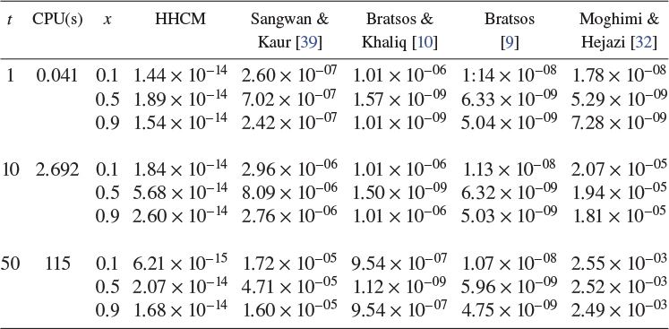
Comparison of absolute error of Example 6.1 for
 $\alpha =0.001,~\beta =0.001,~\varepsilon =1$
,
 $h=0.1$
and
 $\Delta t=0.0001$
.

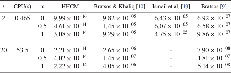
Comparison of absolute error of Example 6.1 for
 $\varepsilon =1$
,
 $\alpha =0.01,~ \beta =0.01$
,
 $h=0.1$
and
 $\Delta t=0.0002$
.

In Tables 1–5, comparison of the absolute error with the variational iteration method [Reference Moghimi and Hejazi32], exponentially fitted technique [Reference Sangwan and Kaur39], exponential time differencing scheme [Reference Bratsos and Khaliq10], Adomian decomposition method [Reference Ismail, Raslan and Rabboh19], compact finite difference method [Reference Sari, Gurarslan and Dag40], finite element method [Reference Yadav and Jiwari45], homotopy perturbation method [Reference Babolian and Saeidian6] and modified predictor–corrector method [Reference Bratsos9] is given at different time levels for different values of
 $\alpha , ~\beta $
and
 $\varepsilon $
. Comparison of maximum absolute error with spectral domain decomposition [Reference Golbabai and Javidi18], cubic B-splines collocation technique [Reference Mittal and Tripathi31] and local discontinuous Galerkin method [Reference Zhang, Yu and Zhao46] is given in Table 6, and time and space orders of convergence are given in Tables 7 and 8. It is observed that the present results are better than those of previous investigators. In Figure 1, plots for different values of
 $\varepsilon =2^{-4},2^{-8}, 2^{-12}, 2^{-16}$
are drawn at different time levels
 $t=0.1,0.5,1,5,10$
. In all these plots, it is clear that the sharper boundary layers appear to occur at the left-hand side of the domain as singular perturbation parameter
 $\varepsilon $
becomes increasingly smaller. All the plots depict efficiency and robustness of the HHCM technique in capturing the boundary layers very sharply.
Comparison of absolute error of Example 6.1 for
 $\varepsilon =1$
,
 $\alpha =1,~ \beta =0$
,
 $h=0.1$
and
 $\Delta t=0.0001$
.

Absolute error of Example 6.1 for
 $\alpha =0.01,~\beta =0.01,~\varepsilon =1$
,
 $h=0.5$
and
 $\Delta t=0.0001$
.

Comparison of absolute error of Example 6.1 for
 $\varepsilon =1$
,
 $h=0.1$
and
 $\Delta t=0.000\,01$
.

Comparison of maximum absolute error of Example 6.1 for
 $\varepsilon =1$
,
 $h=0.1$
and
 $\Delta t=0.000\,01$
.

Time rate convergence of Example 6.1 for
 $\varepsilon =1$
,
 $h=0.1$
.

Space rate convergence of Example 6.1 for
 $\varepsilon =2^{-17}$
,
 $\Delta t=0.001$
,
 $\alpha =0.01,~ \beta =0.01,~ t=1$
.

 $\varepsilon $
-effect, time-effect and comparison of exact and numerical solutions of Example 6.1 with
 $h=0.1$
,
 $\Delta t=0.001$
,
 $\alpha =0.01$
and
 $\beta =0.01$
.

6.2 Fisher equation (FE)
Example 6.2. Consider equations (1.1)–(1.3) with
 $\alpha =0$
and initial condition
 $$ \begin{align*} u(x,0)=\big(1+e^{\big[\sqrt{{\beta}/{6}}\,x\big]}\big)^{-2} \end{align*} $$
and boundary conditions
 $$ \begin{align*} \lim_{x \rightarrow -\infty}u(x,t)=1,\quad \lim_{x \rightarrow +\infty}u(x,t)=0. \end{align*} $$
The analytic solution is proposed by Ablowitz and Zeppetella [Reference Ablowitz and Zeppetella1] as
 $$ \begin{align*} u(x,t)=\big(1+e^{\big[\sqrt{{\beta}/{6}}\,x-({5\beta}/{6})t\big]}\big)^{-2}. \end{align*} $$
The computational analysis is performed in the space domain
 $[-0.2,0.8]$
. In Tables 9 and 10, comparisons of
 $L_2$
and
 $L_{\infty }$
with the exponential cubic B-spline method [Reference Dag and Ersoy14], moving mesh method [Reference Qiu and Sloan35], B-spline Galerkin method [Reference Dag, Sahin and Korkmaz15], cubic B-spline collocation method [Reference Rohila and Mittal36], cubic trigonometric B-spline differential quadrature method [Reference Tamsir, Dhiman and Srivastava42], extended modified cubic B-spline [Reference Shuklav and Tamsir41] and Crank–Nicholson finite difference scheme (CN), accurate space derivatives (ASD) and discrete singular convolution (DSC) [Reference Zhao and Wei47] are given for different values of
 $\varepsilon =1$
and
 $\beta =1,6,10\,000$
.
Comparison of
 $L_2$
and
 $L_{\infty }$
errors of Example 6.2 for
 $\Delta t=0.1$
.

Comparison of
 $L_{2}$
and
 $L_{\infty } $
error of Example 6.2 with
 $N=64$
,
 $\Delta t=0.000\,005$
,
 $\varepsilon =1$
,
 $\beta =10\,000$
.

In Table 9, Rohila and Mittal [Reference Rohila and Mittal36] took the number of element as
 $101$
, but in the present case, only
 $21$
elements are considered. Moreover, HHCM gives better result as compared with the cubic B-spline collocation method [Reference Rohila and Mittal36] and other previous investigations. The
 $L_2$
and
 $L_{\infty }$
errors are given in Table 11 for
 $\varepsilon =1$
,
 $\beta =6$
and different values of time step
 $\Delta t=0.01,0.001,0.000\,1,0.000\,01$
and time
 $t=0.15,0.35,0.55,0.75,0.95$
. In Table 12, the time rate convergence is given. In Figure 2, exact and numerical solution are plotted for different time levels
 $t=0.001,0.002,0.003,0.004$
and
 $\beta =2000,5000$
. A surface plot of numerical solution is given in Figure 3.
 $L_{2}$
and
 $L_{\infty } $
error of Example 6.2 with
 $\varepsilon =1$
,
 $\beta =6$
and
 $N=20$
.

Time rate convergence of Example 6.2 for
 $ \varepsilon =1$
,
 $N=21$
.

Example 6.3. Consider the Fisher equation [Reference Shuklav and Tamsir41]
 $$ \begin{align*} u_t=\varepsilon u_{xx}+ zu^2-su,\quad 0<t<\infty, \quad \infty<x<\infty \end{align*} $$
with boundary conditions
 $$ \begin{align*} \lim_{x \rightarrow -\infty}u(x,t)=0.5,\quad \lim_{x \rightarrow +\infty}u(x,t)=0. \end{align*} $$
The analytic solution is given by
 $$ \begin{align*} u(x,t)=-\frac{s}{4z}\bigg[\text{sech}^2\bigg(\pm\sqrt{\frac{s}{24v}}x+\frac{5s}{12}t\bigg) -2\tanh\bigg(\pm\sqrt{\frac{s}{24v}}x+\frac{5s}{12}t\bigg)-2\bigg]. \end{align*} $$
In Table 13, comparison of absolute error with the modified cubic B-spline collocation method [Reference Mittal and Jain29], extended modified cubic B-spline [Reference Shuklav and Tamsir41], B-spline method [Reference Cattani and Kudreyko12, Reference Mittal and Arora28], cubic trigonometric B-spline differential quadrature method [Reference Tamsir, Dhiman and Srivastava42] is given. In Table 14, time rate convergence is given. Behaviours of the exact and numeric solutions for different time levels
 $t=1,2,3,4,5$
are plotted in Figure 4. In Figure 5, plots of absolute error for
 $t=1,3,5,7,9$
are drawn.
Comparison of exact and numerical solutions of Example 6.2 with
 $h=0.025$
,
 $\Delta t=0.000\,01$
and
 $\varepsilon =1$
.

Surface plot of solution of Example 6.2 with
 $h=0.025$
,
 $\Delta t=0.000\,01$
,
 $\varepsilon =1$
and
 $\beta =10\,000$
.

Comparison of absolute error of Example 6.3 at
 $t=4$
with
 $h=0.25$
,
 $\Delta t=0.01$
,
 $s=0.5$
,
 $z=1$
,
 $v=1$
.

Time rate convergence of Example 6.3 for
 $\varepsilon =1$
,
 $h=0.25$
.

Comparison of exact and numerical solutions of Example 6.3 with
 $h=0.5$
,
 $\Delta t=0.01$
,
 $\varepsilon =1$
,
 $s=0.5$
,
 $z=1$
and
 $v=1$
.

7 Conclusion
The hepta Hermite collocation method with the Crank–Nicholson scheme is used to solve the nonlinear Fisher and BF equations. The quasilinearization process is used to deal with nonlinear terms. Suitable examples are solved with the proposed technique to show the efficacy and improvement in the numerical results. The von Neumann method is used for stability analysis and the proposed scheme is proved to be unconditionally stable. The order of convergence of the proposed method is found to be six in the space domain and two in the temporal domain. From the tables and figures, it is concluded that the HHCM gives more accurate results, as compared with the existing ones. Also, the results show very good agreement with the exact solution. Overall, the study demonstrates the efficacy and stability of the hepta Hermite collocation method.
Absolute error of Example 6.3 with
 $h=0.5$
,
 $\Delta t=0.01$
,
 $\varepsilon =1$
,
 $s=0.5$
,
 $z=1$
and
 $v=1$
.