



1 Introduction
This study investigates a circular cylinder with forced oscillation in the streamwise direction in a uniform flow. Flows over bluff bodies have attracted attention not only from the viewpoint of fluid–structure interaction but also from the perspective of flow control due to the wake behind the bluff body. The most common bluff-body shape is a circular cylinder, which is frequently observed in applications such as marine cables, power lines, bridges and buildings. A cylinder in a uniform flow induces unsteady flow, even though the cylinder is in a steady state over a certain range of Reynolds numbers. Unsteady flow for a stationary circular cylinder is observed as periodic vortex shedding, the so-called von Kármán vortex street, and the Strouhal frequency (
 $f_{St}$
) of vortex shedding is determined by the Reynolds number. Because of this periodic vortex shedding, the oscillatory motion of the cylinder is generated by the vortex-induced force acting on the cylinder. A forced oscillating circular cylinder inherently has two frequency components: one is the applied driving frequency and the other is the Strouhal frequency corresponding to the flow over the circular cylinder. These two frequency components can induce synchronization at a certain oscillating condition. The flow of the circular cylinder undergoing forced oscillation showed features very close to those of a freely oscillating cylinder under matched oscillating parameters with such synchronization (Morse & Williamson Reference Morse and Williamson2009; Bearman Reference Bearman2011). Therefore, cylinders undergoing forced oscillation have attracted great interest in terms of the synchronization of fluid and cylinder motion.
Bishop & Hassan (Reference Bishop and Hassan1964) studied the lift force of a flow over a transversely oscillating circular cylinder and summarized its frequency behaviour. When the cylinder oscillated at a driving frequency far from the Strouhal frequency, the lift force was composed of the driving-frequency and Strouhal-frequency components. However, the lift signal was synchronized with the motion of the cylinder as the driving frequency (
 $f_{d}$
) near the Strouhal frequency; therefore, in this case, the lift signal only had a driving-frequency component without a Strouhal-frequency component. This synchronization is also called lock-in because the flow was locked in with the cylinder motion. Many studies on the flow over a transversely oscillating cylinder have focused on the lock-in phenomenon (Koopmann Reference Koopmann1967; Anagnostopoulos Reference Anagnostopoulos2000; Kaiktsis, Triantafyllou & Özbas Reference Kaiktsis, Triantafyllou and Özbas2007). These studies commonly showed that a lock-in phenomenon was found in a frequency range close to
 $f_{d}/f_{St}=1$
, and that this frequency range expanded as the driving amplitude increased. Aerodynamic force in lock-in phenomena for a transversely oscillating cylinder also shows common features. The drag and lift forces show sinusoidal patterns in the lock-in region. The lift force increases in the lock-in region with driving frequency, and the phase between the lift force and cylinder motion shows a sudden change at a critical frequency, which is in the middle of the lock-in frequency range.
Flow over a streamwise oscillating cylinder shows features of lock-in phenomena different from those in the case of a transversely oscillating cylinder. A study on a cylinder freely oscillating simultaneously in the streamwise and transverse directions showed that the oscillating frequency in the streamwise direction is twice that in the transverse direction (Dahl et al.
Reference Dahl, Hover, Triantafyllou and Oakley2010). An experiment on flow over cylinders undergoing forced oscillations in the transverse and streamwise directions was performed by Tanida, Okajima & Watanabe (Reference Tanida, Okajima and Watanabe1973) to observe the lift and drag forces. The transversely oscillating cylinder showed lock-in in a frequency range close to
 $f_{d}/f_{St}=1$
as in previous studies, but the streamwise oscillating cylinder presented lock-in phenomena in a range close to
 $f_{d}/f_{St}=2$
. Griffin & Ramberg (Reference Griffin and Ramberg1976) observed the vortex pattern behind a streamwise oscillating cylinder at various driving amplitudes and frequencies. The lock-in region was found at a driving frequency near
 $f_{d}/f_{St}=2$
, and the frequency range for the lock-in region was expanded as the driving amplitude increased. This expansion of the frequency range for lock-in was also reported in a numerical study (Al-Mdallal, Lawrence & Kocabiyik Reference Al-Mdallal, Lawrence and Kocabiyik2007).
Ongoren & Rockwell (Reference Ongoren and Rockwell1988) performed an experiment on flow over a circular cylinder oscillating at an angle
 $\unicode[STIX]{x1D6FC}$
(
 $\unicode[STIX]{x1D6FC}=0^{\circ },45^{\circ }$
and
 $90^{\circ }$
) with a wide range of driving frequencies (
 $f_{d}/f_{St}=0.5{-}4.0$
) at a fixed amplitude and Reynolds number. They found two separate lock-in regions in the case of streamwise oscillation (
 $\unicode[STIX]{x1D6FC}=0^{\circ }$
): the first lock-in region occurred at a driving frequency close to
 $f_{d}/f_{St}=2$
, which showed a von-Kármán-like asymmetric vortex pattern; and a new lock-in region was found at
 $f_{d}/f_{St}=3$
, which presented a symmetric vortex pattern. Yokoi & Kamemoto (Reference Yokoi and Kamemoto1994) also observed lock-in phenomena that had symmetric vortex patterns. They investigated the average frequency of vortex shedding, and the ratio of the average vortex shedding frequency to driving frequency was
 $n=0.5,1,2,\ldots ,\infty$
at lock-in. The asymmetric vortex pattern was found at
 $n=0.5$
, while the symmetric vortex pattern was formed at
 $n=1$
. Xu, Zhou & Wang (Reference Xu, Zhou and Wang2006) also observed such a symmetric vortex pattern through experiments and explained it using the concept of a relative Reynolds number, in which the Reynolds number has a velocity factor defined as the relative velocity between the flow and the moving cylinder. Barbi et al. (Reference Barbi, Favier, Maresca and Telionis1986) experimentally visualized several vortex patterns in order to describe the lock-in phenomena in cylinder wake flows due to streamwise inflow perturbations. They found that a symmetric vortex pattern was observed at the higher values of driving frequency in the corresponding range for lock-in. Symmetric vortex patterns were also found in previous studies related to the responses of cylinder wake flows to streamwise inflow perturbations (Kim, Yoo & Sung Reference Kim, Yoo and Sung2006; Konstantinidis & Balabani Reference Konstantinidis and Balabani2007a
; Feng & Wang Reference Feng and Wang2010; Konstantinidis & Bouris Reference Konstantinidis and Bouris2016). An additional lock-in region was found by Cetiner & Rockwell (Reference Cetiner and Rockwell2001) from an experiment that observed the lift force history for various driving amplitudes and frequencies, and they classified the lift force signals into three categories (non-lock-in, intermittent lock-in and lock-in). The ordinary lock-in region was found over a frequency range close to
 $f_{d}/f_{St}=2$
, and an additional lock-in region was observed at a driving frequency near
 $f_{d}/f_{St}=1$
when the cylinder oscillated with a large driving amplitude.
An in-depth study of the flow over a streamwise oscillating cylinder for various Reynolds numbers, driving amplitudes and frequencies was performed by Leontini, Jacono & Thompson (Reference Leontini, Jacono and Thompson2011, Reference Leontini, Jacono and Thompson2013). First, they observed the flow over an oscillating cylinder at
 $f_{d}/f_{St}=1$
for various amplitudes, and the lift signals of each amplitude were classified as quasi-periodic (QP), chaotic and P
 $_{n}$
, which denotes the completion of a period of vortex shedding during
 $n$
-cycle cylinder motion, using Poincaré maps. The primary frequency of the quasi-periodic flow spectrum peak was modelled by a power of the driving amplitude
 $(A)$
, and the remaining frequencies of peaks were modelled by
 $f_{d}$
. Furthermore, they observed the relation between the primary frequency (
 $f_{s}$
) of the peak of the quasi-periodic flow spectrum and the
 $f_{d}$
of the cylinder at the lock-in region, which is represented as
 $1/(1-f_{d}/f_{s})=n$
, where
 $n=0,1,2,\ldots ,\infty$
. Subsequent research considered various Reynolds numbers, driving amplitudes and frequencies as factors impacting the primary frequency of vortex shedding. The primary frequency of vortex shedding at QP is proportional to the driving amplitude, and the proportionality constant showed features different from those for the Reynolds number and driving frequency. Using the relation of vortex shedding frequency with driving amplitude, they presented a threshold amplitude for lock-in and thereby predicted a driving amplitude of P
 $_{2}$
.
Previous studies (e.g. Griffin & Ramberg Reference Griffin and Ramberg1976; Ongoren & Rockwell Reference Ongoren and Rockwell1988; Yokoi & Kamemoto Reference Yokoi and Kamemoto1994; Cetiner & Rockwell Reference Cetiner and Rockwell2001; Al-Mdallal Reference Al-Mdallal2004; Xu et al.
Reference Xu, Zhou and Wang2006; Al-Mdallal et al.
Reference Al-Mdallal, Lawrence and Kocabiyik2007; Leontini et al.
Reference Leontini, Jacono and Thompson2011, Reference Leontini, Jacono and Thompson2013) indicated that there are several lock-in regions, and that these additional lock-in regions are distributed in separate ranges depending on the driving amplitude and frequency. These previous conclusions suggest that investigating a narrow range of driving amplitudes and frequencies may be insufficient for the understanding of the features of lock-in behaviour. Therefore, a comprehensive study of the effects of both the driving amplitude and frequency on the lock-in region is necessary. In this study, two-dimensional flows induced by an oscillating cylinder placed in the streamwise direction are observed in terms of various driving amplitudes and frequencies. As the baseline flow condition, we consider flows having low or moderate Reynolds numbers (up to
 $Re=200$
) for a stationary circular cylinder. It should be noted that a two-dimensional approximation of flows may not be valid for a case involving large-amplitude oscillations. For two-dimensional flow approximations, many researchers (including Blackburn & Henderson Reference Blackburn and Henderson1999; Anagnostopoulos Reference Anagnostopoulos2000; Al-Mdallal Reference Al-Mdallal2004; Al-Mdallal et al.
Reference Al-Mdallal, Lawrence and Kocabiyik2007; Kaiktsis et al.
Reference Kaiktsis, Triantafyllou and Özbas2007; Leontini et al.
Reference Leontini, Jacono and Thompson2011) have investigated the lock-in phenomenon for flow over an oscillating cylinder at moderate Reynolds numbers (even at
 $Re=500$
). However, in this work, we have primarily focused on the effects of driving amplitude and frequency on the lock-in phenomenon for two-dimensional flows over a streamwise oscillating cylinder. A lift coefficient spectrum is used to define the lock-in region, and it is found that there are two types of lock-in phenomena, which are classified according to the frequency of peaks of the lift coefficient spectrum into subharmonic lock-in and harmonic lock-in. Each driving amplitude and frequency that generates lock-in phenomena is marked on the driving amplitude–frequency plane to obtain a lock-in region map, which shows separate lock-in regions categorized as subharmonic or harmonic. The distribution of each lock-in region with respect to the driving amplitude and frequency is observed, and the lower boundary of the subharmonic region is predicted following the model presented by Leontini et al. (Reference Leontini, Jacono and Thompson2013). Furthermore, the vortex pattern of each region is observed to explain fluid interactions with the cylinder, and these vortex effects in each region are represented on aerodynamic force maps that show the mean and root-mean-square (r.m.s.) values of aerodynamic force on the driving amplitude–frequency plane. The effect of Reynolds number is verified by the lock-in region maps and aerodynamic force maps for
 $Re=40$
and
 $Re=200$
, which are compared with the results for
 $Re=100$
.
2 Governing equations
The two-dimensional incompressible Navier–Stokes and continuity equations in a non-inertial system are used in polar coordinates. The transformation to the non-inertial system produces the inertial force terms in the momentum equation. The governing equations are thus expressed as follows:
 $$\begin{eqnarray}\displaystyle & \displaystyle \frac{\unicode[STIX]{x2202}u_{r}}{\unicode[STIX]{x2202}t}+\frac{\unicode[STIX]{x2202}u_{r}u_{r}}{\unicode[STIX]{x2202}r}+\frac{u_{r}u_{r}-u_{\unicode[STIX]{x1D703}}u_{\unicode[STIX]{x1D703}}}{r}+\frac{1}{r}\frac{\unicode[STIX]{x2202}u_{r}u_{\unicode[STIX]{x1D703}}}{\unicode[STIX]{x2202}\unicode[STIX]{x1D703}}=-\frac{\unicode[STIX]{x2202}p}{\unicode[STIX]{x2202}r}+\frac{1}{Re}\left(\unicode[STIX]{x1D6FB}^{2}u_{r}-\frac{2}{r^{2}}\frac{\unicode[STIX]{x2202}u_{\unicode[STIX]{x1D703}}}{\unicode[STIX]{x2202}\unicode[STIX]{x1D703}}-\frac{u_{r}}{r^{2}}\right)-a_{r}, & \displaystyle \nonumber\\ \displaystyle & & \displaystyle\end{eqnarray}$$
 $$\begin{eqnarray}\displaystyle & \displaystyle \frac{\unicode[STIX]{x2202}u_{\unicode[STIX]{x1D703}}}{\unicode[STIX]{x2202}t}+\frac{\unicode[STIX]{x2202}u_{r}u_{\unicode[STIX]{x1D703}}}{\unicode[STIX]{x2202}r}+2\frac{u_{r}u_{r}}{r}+\frac{1}{r}\frac{\unicode[STIX]{x2202}u_{\unicode[STIX]{x1D703}}u_{\unicode[STIX]{x1D703}}}{\unicode[STIX]{x2202}\unicode[STIX]{x1D703}}=-\frac{1}{r}\frac{\unicode[STIX]{x2202}p}{\unicode[STIX]{x2202}\unicode[STIX]{x1D703}}+\frac{1}{Re}\left(\unicode[STIX]{x1D6FB}^{2}u_{\unicode[STIX]{x1D703}}+\frac{2}{r^{2}}\frac{\unicode[STIX]{x2202}u_{r}}{\unicode[STIX]{x2202}\unicode[STIX]{x1D703}}-\frac{u_{\unicode[STIX]{x1D703}}}{r^{2}}\right)-a_{\unicode[STIX]{x1D703}}, & \displaystyle\end{eqnarray}$$
 $$\begin{eqnarray}\displaystyle & \displaystyle \frac{\unicode[STIX]{x2202}u_{r}}{\unicode[STIX]{x2202}r}+\frac{u_{r}}{r}+\frac{1}{r}\frac{\unicode[STIX]{x2202}u_{\unicode[STIX]{x1D703}}}{\unicode[STIX]{x2202}\unicode[STIX]{x1D703}}=0. & \displaystyle\end{eqnarray}$$
Here,
 $u_{r}$
and
 $u_{\unicode[STIX]{x1D703}}$
are the dimensionless radial and azimuthal velocity components, respectively;
 $p$
is the dimensionless pressure; and
 $a_{r}$
and
 $a_{\unicode[STIX]{x1D703}}$
are dimensionless radial and azimuthal components of cylinder acceleration (
 $\boldsymbol{a}_{cyl}$
), respectively, which gives the inertial force. The following non-dimensionalization is employed:
 $$\begin{eqnarray}t=\frac{\hat{t}U_{0}}{D},\quad r=\frac{\hat{r}}{D},\quad u_{r}=\frac{\hat{u_{r}}}{U_{0}},\quad u_{\unicode[STIX]{x1D703}}=\frac{\hat{u_{\unicode[STIX]{x1D703}}}}{U_{0}},\quad p=\frac{\hat{p}}{\unicode[STIX]{x1D70C}{U_{0}}^{2}},\quad a_{r}=\frac{\hat{a_{r}}D}{{U_{0}}^{2}},\quad a_{\unicode[STIX]{x1D703}}=\frac{\hat{a_{\unicode[STIX]{x1D703}}}D}{{U_{0}}^{2}}.\end{eqnarray}$$
Here
 $U_{0}$
is the free-stream velocity in the inertial system;
 $D$
is the diameter of the cylinder;
 $\unicode[STIX]{x1D70C}$
is the fluid density; and the symbol
 $\hat{~}$
indicates a dimensional variable. The Reynolds number is
 $Re=U_{0}D/\unicode[STIX]{x1D708}$
, where
 $U_{0}$
is the free-stream velocity in the inertial system,
 $D$
is the diameter of the cylinder and
 $\unicode[STIX]{x1D708}$
is the kinematic viscosity. The Laplace operator,
 $\unicode[STIX]{x1D6FB}^{2}$
, is
 $$\begin{eqnarray}\displaystyle \unicode[STIX]{x1D6FB}^{2}=\frac{\unicode[STIX]{x2202}^{2}}{\unicode[STIX]{x2202}r^{2}}+\frac{1}{r}\frac{\unicode[STIX]{x2202}}{\unicode[STIX]{x2202}r}+\frac{1}{r^{2}}\frac{\unicode[STIX]{x2202}^{2}}{\unicode[STIX]{x2202}\unicode[STIX]{x1D703}^{2}}. & & \displaystyle\end{eqnarray}$$
Computational domain in the coordinate systems for flow over a streamwise oscillatory circular cylinder.
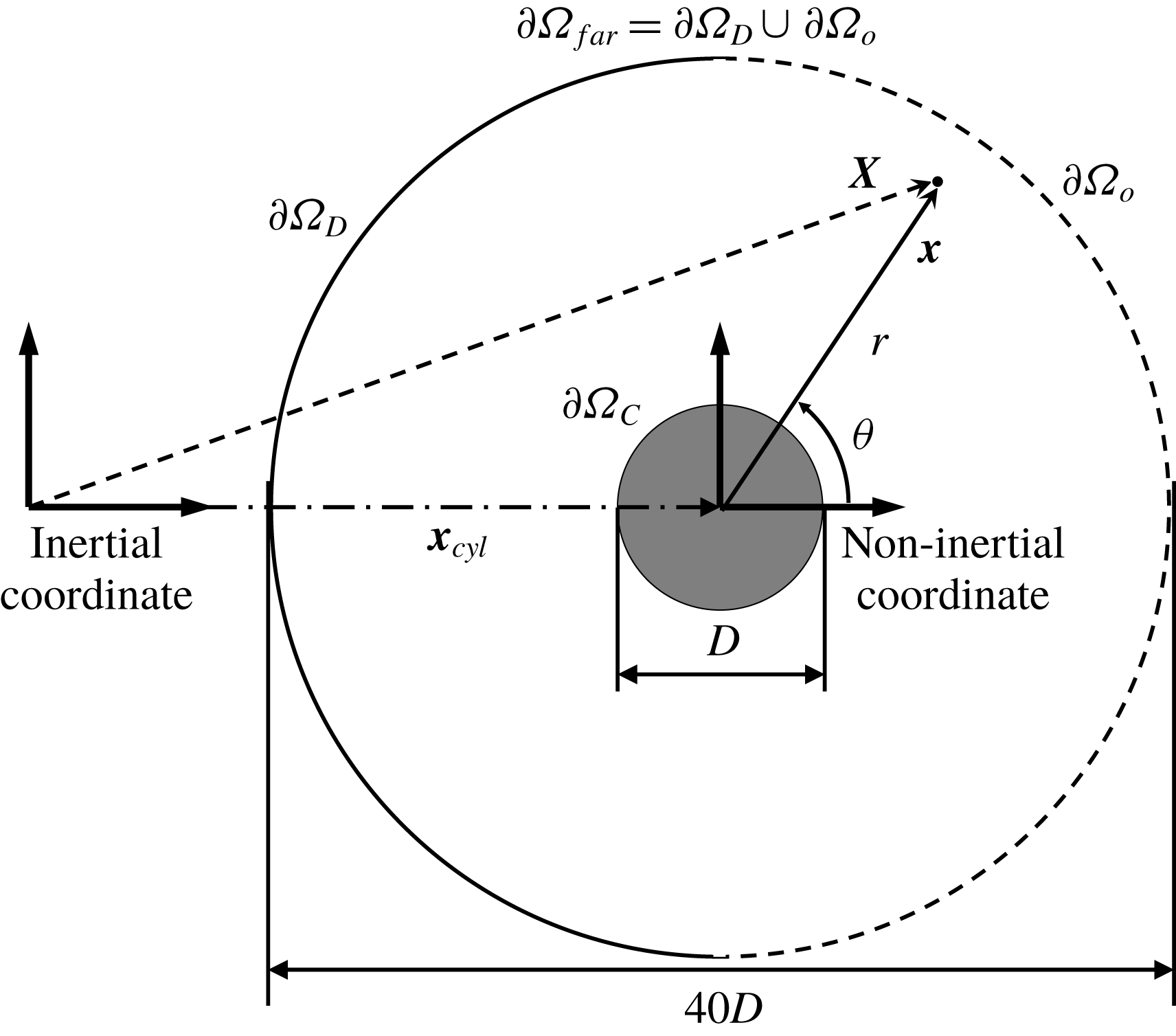
Figure 1 shows the physical model and coordinate systems of the streamwise oscillating cylinder in the free stream. The non-inertial system, which moves with the cylinder, is used to represent the motion of the cylinder, and the non-inertial coordinate is denoted by
 $\boldsymbol{x}$
. Momentum is conserved in the inertial system
 $\boldsymbol{X}$
. The non-inertial and inertial systems have the following relationship:
 $$\begin{eqnarray}\displaystyle \boldsymbol{X}=\boldsymbol{x}+\boldsymbol{x}_{cyl}, & & \displaystyle\end{eqnarray}$$
where
 $\boldsymbol{x}_{cyl}$
is the position of the accelerating non-inertial system, which is the same as the cylinder position. In this study, the cylinder has a streamwise forced oscillating motion,
 $$\begin{eqnarray}\displaystyle x_{cyl}=A\sin (2\unicode[STIX]{x03C0}f_{d}t), & & \displaystyle\end{eqnarray}$$
where
 $x_{cyl}$
is the streamwise component of
 $\boldsymbol{x}_{cyl}$
in Cartesian coordinates, and
 $A$
and
 $f_{d}$
are the driving amplitude and frequency of the cylinder, respectively. The dimensionless velocity
 $\boldsymbol{U}$
of a fluid in the inertial system can be expressed as
 $$\begin{eqnarray}\displaystyle \boldsymbol{U}=\boldsymbol{u}+\boldsymbol{u}_{cyl}, & & \displaystyle\end{eqnarray}$$
where
 $\boldsymbol{u}$
is the dimensionless velocity in the non-inertial system and
 $\boldsymbol{u}_{cyl}$
is the dimensionless velocity of the system, which is the same as that of the cylinder motion:
 $u_{cyl}=U_{cyl}/U_{0}\cos (2\unicode[STIX]{x03C0}f_{d}t)$
and
 $v_{cyl}=0$
, where
 $u_{cyl}$
and
 $v_{cyl}$
represent streamwise and transverse components of
 $\boldsymbol{u}_{cyl}$
, respectively. Note that
 $U_{cyl}=2\unicode[STIX]{x03C0}f_{d}A$
is the magnitude of the velocity of the cylinder motion. The streamwise and transverse components of the initial velocity field are set to
 $(1,0)$
in the inertial system, and so the initial velocity field in the non-inertial system can be written as
 $$\begin{eqnarray}u_{r}(r,\unicode[STIX]{x1D703})=(1-U_{cyl}/U_{0})\cos \unicode[STIX]{x1D703},\quad u_{\unicode[STIX]{x1D703}}(r,\unicode[STIX]{x1D703})=-(1-U_{cyl}/U_{0})\sin \unicode[STIX]{x1D703}.\end{eqnarray}$$
In order to guarantee the divergence-free condition and numerical stability within the computational domain, the outflow boundary condition is modified for numerical simulations on open-bounded domains
 $(\unicode[STIX]{x1D6FA})$
with inner boundary
 $\unicode[STIX]{x2202}\unicode[STIX]{x1D6FA}_{C}$
and outer boundary
 $\unicode[STIX]{x2202}\unicode[STIX]{x1D6FA}_{far}$
. The velocity on the inner boundary
 $\unicode[STIX]{x2202}\unicode[STIX]{x1D6FA}_{C}$
is prescribed to have a no-slip condition, which implies that
 $\boldsymbol{u}=0$
. We assume
 $\unicode[STIX]{x2202}\unicode[STIX]{x1D6FA}_{far}=\unicode[STIX]{x2202}\unicode[STIX]{x1D6FA}_{d}\cup \unicode[STIX]{x2202}\unicode[STIX]{x1D6FA}_{o}$
, where
 $\unicode[STIX]{x2202}\unicode[STIX]{x1D6FA}_{d}$
and
 $\unicode[STIX]{x2202}\unicode[STIX]{x1D6FA}_{o}$
represent the inflow and outflow boundaries, respectively. The velocity
 $\boldsymbol{u}$
on
 $\unicode[STIX]{x2202}\unicode[STIX]{x1D6FA}_{d}$
is prescribed as
 $\boldsymbol{u}=\boldsymbol{U}|_{\unicode[STIX]{x2202}\unicode[STIX]{x1D6FA}_{d}}-\boldsymbol{u}_{cyl}$
, where the streamwise and transverse components of
 $\boldsymbol{U}|_{\unicode[STIX]{x2202}\unicode[STIX]{x1D6FA}_{d}}$
are
 $U|_{\unicode[STIX]{x2202}\unicode[STIX]{x1D6FA}_{d}}=1$
and
 $V|_{\unicode[STIX]{x2202}\unicode[STIX]{x1D6FA}_{d}}=0$
, respectively, whereas
 $\boldsymbol{u}$
is unknown on
 $\unicode[STIX]{x2202}\unicode[STIX]{x1D6FA}_{o}$
. To ensure that the emission of the energy influx is in the domain, we use a convective boundary condition at the open boundary of the domain
 $(\unicode[STIX]{x2202}\unicode[STIX]{x1D6FA}_{o})$
, which gives
 $$\begin{eqnarray}\displaystyle \frac{\unicode[STIX]{x2202}\boldsymbol{U}}{\unicode[STIX]{x2202}t}+c\frac{\unicode[STIX]{x2202}\boldsymbol{U}}{\unicode[STIX]{x2202}X}=0, & & \displaystyle\end{eqnarray}$$
where
 $\boldsymbol{U}$
is the velocity of a fluid in the inertial system,
 $\unicode[STIX]{x2202}/\unicode[STIX]{x2202}X$
is a partial differential in the free-stream direction and
 $c$
is the space-averaged exit velocity.
3 Numerical method
3.1 Projection method
The governing equations in polar coordinates have coupled velocity components not only in the convective terms but also in the diffusion terms. The velocity-components decoupled projection method (Kim, Baek & Sung Reference Kim, Baek and Sung2002; Pan et al. Reference Pan, Lee, Kim and Choi2016) is used to avoid an iterative procedure in solving the governing equations. The Crank–Nicolson scheme is applied to the governing equations in time so that they are implicitly discretized. A staggered MAC (marker and cell) mesh, in which the pressure and velocities are placed at the centres and interfaces of cells, respectively, is used for spatial discretization, and the second-order central finite difference scheme is applied in space. The discrete form of the governing equations can be expressed as
 $$\begin{eqnarray}\displaystyle & \displaystyle \frac{\boldsymbol{u}^{n+1}-\boldsymbol{u}^{n}}{\unicode[STIX]{x0394}t}+\unicode[STIX]{x1D649}\boldsymbol{u}^{n+1}=-\unicode[STIX]{x1D642}p^{n+1/2}+\frac{1}{2Re}(\unicode[STIX]{x1D647}\boldsymbol{u}^{n+1}+\unicode[STIX]{x1D647}\boldsymbol{u}^{n})-\boldsymbol{F}, & \displaystyle\end{eqnarray}$$
 $$\begin{eqnarray}\displaystyle & \displaystyle \unicode[STIX]{x1D63F}\boldsymbol{u}^{n+1}=0, & \displaystyle\end{eqnarray}$$
where discrete operators
 $\unicode[STIX]{x1D642}$
,
 $\unicode[STIX]{x1D647}$
and
 $\unicode[STIX]{x1D63F}$
are the gradient, Laplacian and divergence operators, respectively, and
 $\boldsymbol{F}$
is the inertial force vector. The discrete operator
 $\unicode[STIX]{x1D649}$
is a linearized convective operator, where the nonlinear convective term is linearized with second-order temporal accuracy. Here,
 $\unicode[STIX]{x0394}t$
is the discretized time step, and the superscript
 $n$
represents the
 $n$
th time step. The discretized equations can be represented in matrix form as follows:
 $$\begin{eqnarray}\displaystyle \left(\begin{array}{@{}cc@{}}\unicode[STIX]{x1D63C} & \unicode[STIX]{x1D642}\\ \unicode[STIX]{x1D63F} & 0\end{array}\right)\left(\begin{array}{@{}c@{}}\boldsymbol{u}^{n+1}\\ \unicode[STIX]{x1D6FF}p\end{array}\right)=\left(\begin{array}{@{}c@{}}\boldsymbol{R}\\ 0\end{array}\right), & & \displaystyle\end{eqnarray}$$
where
 $$\begin{eqnarray}\displaystyle & \displaystyle \unicode[STIX]{x1D63C}=\frac{1}{\unicode[STIX]{x0394}t}\left[\unicode[STIX]{x1D644}+\unicode[STIX]{x0394}t\left(\unicode[STIX]{x1D649}-\frac{1}{2Re}\unicode[STIX]{x1D647}\right)\right], & \displaystyle\end{eqnarray}$$
 $$\begin{eqnarray}\displaystyle & \displaystyle \boldsymbol{R}=\frac{1}{\unicode[STIX]{x0394}t}\boldsymbol{u}^{n}-\unicode[STIX]{x1D642}p^{n-1/2}+\frac{1}{2Re}\unicode[STIX]{x1D647}\boldsymbol{u}^{n}-\boldsymbol{F}, & \displaystyle\end{eqnarray}$$
 $$\begin{eqnarray}\displaystyle & \displaystyle \unicode[STIX]{x1D6FF}p=p^{1+1/2}-p^{1-1/2}. & \displaystyle\end{eqnarray}$$
The velocity vector and pressure are decoupled based on an approximate block LU decomposition. The procedure of velocity–pressure decoupling can be simplified as follows:
 $$\begin{eqnarray}\displaystyle & \displaystyle \unicode[STIX]{x1D63C}\boldsymbol{u}^{\ast }=\boldsymbol{R}, & \displaystyle\end{eqnarray}$$
 $$\begin{eqnarray}\displaystyle & \displaystyle \unicode[STIX]{x0394}t\unicode[STIX]{x1D63F}\unicode[STIX]{x1D642}\unicode[STIX]{x1D6FF}p=\unicode[STIX]{x1D63F}\boldsymbol{u}^{\ast }, & \displaystyle\end{eqnarray}$$
 $$\begin{eqnarray}\displaystyle & \displaystyle \boldsymbol{u}^{n+1}=\boldsymbol{u}^{\ast }-\unicode[STIX]{x0394}t\unicode[STIX]{x1D642}\unicode[STIX]{x1D6FF}p, & \displaystyle\end{eqnarray}$$
 $$\begin{eqnarray}\displaystyle & \displaystyle p^{1+1/2}=p^{1-1/2}+\unicode[STIX]{x1D6FF}p, & \displaystyle\end{eqnarray}$$
where
 $\boldsymbol{u}^{\ast }$
is the intermediate velocity of
 $\boldsymbol{u}^{n+1}$
. The operator
 $\unicode[STIX]{x1D63C}$
in (3.7) is expressed as
 $$\begin{eqnarray}\displaystyle \unicode[STIX]{x1D63C}=\frac{1}{\unicode[STIX]{x0394}t}\left(\begin{array}{@{}cc@{}}\unicode[STIX]{x1D644}+\unicode[STIX]{x0394}t\unicode[STIX]{x1D648}_{11} & \unicode[STIX]{x0394}t\unicode[STIX]{x1D648}_{12}\\ \unicode[STIX]{x0394}t\unicode[STIX]{x1D648}_{21} & \unicode[STIX]{x1D644}+\unicode[STIX]{x0394}t\unicode[STIX]{x1D648}_{22}\end{array}\right), & & \displaystyle\end{eqnarray}$$
where
 $\unicode[STIX]{x1D648}_{ij}$
is a submatrix
 $\unicode[STIX]{x1D648}=\unicode[STIX]{x1D649}-(1/(2Re))\unicode[STIX]{x1D647}$
in which the off-diagonal matrix
 $\unicode[STIX]{x1D648}$
is non-zero because of coupled velocity components not only in convection terms but also in the diffusion terms in polar coordinates. By applying block LU decomposition along with approximate factorization, velocity components are decoupled, and the intermediate velocity can be calculated in the following step using new variables
 $\unicode[STIX]{x1D6FF}\boldsymbol{u}^{\ast \ast }$
without iteration:
 $$\begin{eqnarray}\displaystyle & \displaystyle \frac{1}{\unicode[STIX]{x0394}t}(\unicode[STIX]{x1D644}+\unicode[STIX]{x0394}t\unicode[STIX]{x1D648}_{11})\unicode[STIX]{x1D6FF}u_{1}^{\ast \ast }=R_{1}^{\ast }, & \displaystyle\end{eqnarray}$$
 $$\begin{eqnarray}\displaystyle & \displaystyle \frac{1}{\unicode[STIX]{x0394}t}(\unicode[STIX]{x1D644}+\unicode[STIX]{x0394}t\unicode[STIX]{x1D648}_{22})\unicode[STIX]{x1D6FF}u_{2}^{\ast \ast }=R_{2}^{\ast }-\unicode[STIX]{x1D648}_{21}u_{1}^{\ast \ast }, & \displaystyle\end{eqnarray}$$
 $$\begin{eqnarray}\displaystyle & \displaystyle \unicode[STIX]{x1D6FF}u_{2}^{\ast }=\unicode[STIX]{x1D6FF}u_{2}^{\ast \ast }, & \displaystyle\end{eqnarray}$$
 $$\begin{eqnarray}\displaystyle & \displaystyle \unicode[STIX]{x1D6FF}u_{1}^{\ast }=\unicode[STIX]{x1D6FF}u_{1}^{\ast \ast }-\unicode[STIX]{x0394}t\unicode[STIX]{x1D648}_{12}u_{2}^{\ast }, & \displaystyle\end{eqnarray}$$
where
 $\boldsymbol{R}^{\ast }=-\unicode[STIX]{x1D63C}\boldsymbol{u}^{n}+\boldsymbol{R}$
.
3.2 Poisson equation solver
The Poisson equation (3.8) needs to be solved at every time step to project the velocity field onto a divergence-free space. For simplicity, our equation (3.8) can be replaced by the following simple form:
 $$\begin{eqnarray}\displaystyle \unicode[STIX]{x1D647}\unicode[STIX]{x1D6FF}p=R_{p}. & & \displaystyle\end{eqnarray}$$
Here,
 $\unicode[STIX]{x1D647}=\unicode[STIX]{x1D63F}\unicode[STIX]{x1D642}$
is the Laplacian operator,
 $\unicode[STIX]{x1D6FF}p$
is the pressure increment and
 $R_{p}$
is the right-hand side of the Poisson equation (3.8). Owing to the non-local nature of its solution, this elliptic system is one of the most time-consuming parts of the computation. In order to reduce the computational time, a direct Poisson solver is used: a restricted Poisson solver for problems with one uniform periodic direction based on the Fourier diagonalization technique along the periodic direction. When we apply the Fourier transform to
 $\unicode[STIX]{x1D647}$
, the Laplacian operator in the spectral space,
 $\hat{\unicode[STIX]{x1D647}}$
, is obtained. Note that the Fourier-transformed
 $\unicode[STIX]{x1D703}$
-directional differential operator in
 $\hat{\unicode[STIX]{x1D647}}$
only has
 $\unicode[STIX]{x1D706}_{k}$
on its diagonal, which is given by
 $$\begin{eqnarray}\displaystyle \unicode[STIX]{x1D706}_{k}=-\frac{1}{\unicode[STIX]{x03C0}}\left(1-\cos \left(\frac{2\unicode[STIX]{x03C0}k}{N_{\unicode[STIX]{x1D703}}}\right)\right)\quad \text{for}~k=0,1,\ldots ,N_{\unicode[STIX]{x1D703}}/2, & & \displaystyle\end{eqnarray}$$
where
 $N_{\unicode[STIX]{x1D703}}$
is the number of grid points in the azimuthal direction. Therefore, the original system in (3.16) is decomposed into a set of mutually independent one-dimensional systems
 $\hat{\unicode[STIX]{x1D647}}\hat{\unicode[STIX]{x1D6FF}p}=\hat{R_{p}}$
where the superscript
 $\hat{}$
indicates Fourier-transformed variables. In summary, we solve the Poisson equation by using the following procedure.
(i) Apply Fourier transform to the right-hand side
 $R_{p}$
:
$\hat{R_{p}}={\mathcal{F}}(R_{p})$
.
(ii) Solve the transformed one-dimensional systems:
$\hat{\unicode[STIX]{x1D647}}\hat{\unicode[STIX]{x1D6FF}p}=\hat{R_{p}}$
.(iii) Apply inverse Fourier transform to the solution:
$\unicode[STIX]{x1D6FF}p={\mathcal{F}}^{\ast }(\hat{\unicode[STIX]{x1D6FF}p})$
.


Here
 ${\mathcal{F}}$
and
 ${\mathcal{F}}^{\ast }$
are the Fourier transform and its inverse, respectively.
3.3 Details of numerical simulations
We can prescribe the outflow boundary condition (2.10) while controlling energy growth in the domain as follows:
 $$\begin{eqnarray}\displaystyle \boldsymbol{U}^{n+1}=\boldsymbol{U}^{n}-c\unicode[STIX]{x0394}t\frac{\unicode[STIX]{x2202}\boldsymbol{U}^{n}}{\unicode[STIX]{x2202}X}. & & \displaystyle\end{eqnarray}$$
However, this boundary condition fails to guarantee the divergence-free condition of the velocity in the domain; therefore, an additional mass-correction process is needed. It is clear from the continuity equation (2.3) that we have
 $\int _{\unicode[STIX]{x1D6FA}}\unicode[STIX]{x1D735}\boldsymbol{\cdot }\boldsymbol{U}^{n+1}=0$
, and this condition should also be satisfied in the inertial system. The divergence theorem allows us to rewrite this equation as
 $$\begin{eqnarray}\displaystyle \int _{\unicode[STIX]{x1D6FA}}\unicode[STIX]{x1D735}\boldsymbol{\cdot }\boldsymbol{U}^{n+1}=\int _{\unicode[STIX]{x2202}\unicode[STIX]{x1D6FA}_{d}}\boldsymbol{U}^{n+1}\boldsymbol{\cdot }\boldsymbol{n}+\int _{\unicode[STIX]{x2202}\unicode[STIX]{x1D6FA}_{o}}\boldsymbol{U}^{n+1}\boldsymbol{\cdot }\boldsymbol{n}, & & \displaystyle\end{eqnarray}$$
where
 $\unicode[STIX]{x2202}\unicode[STIX]{x1D6FA}_{d}$
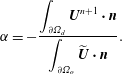
is the inflow boundary. By introducing a mass-correction procedure, a convective boundary condition in the far field is used to maintain energy and conserve mass in the computational domain. The mass-correction process is as follows:
(i) Calculate an intermediate velocity at the open boundary
$\unicode[STIX]{x2202}\unicode[STIX]{x1D6FA}_{o}$
, (3.20)$$\begin{eqnarray}\widetilde{\boldsymbol{U}}\big|_{\unicode[STIX]{x2202}\unicode[STIX]{x1D6FA}_{o}}=\boldsymbol{U}^{n}\big|_{\unicode[STIX]{x2202}\unicode[STIX]{x1D6FA}_{o}}-\left.c\unicode[STIX]{x0394}t\frac{\unicode[STIX]{x2202}\boldsymbol{U}^{n}}{\unicode[STIX]{x2202}X}\right|_{\unicode[STIX]{x2202}\unicode[STIX]{x1D6FA}_{o}}.\end{eqnarray}$$
(ii) Define a correction factor
$\unicode[STIX]{x1D6FC}$
, (3.21)$$\begin{eqnarray}\unicode[STIX]{x1D6FC}=-\frac{\displaystyle \int _{\unicode[STIX]{x2202}\unicode[STIX]{x1D6FA}_{d}}\boldsymbol{U}^{n+1}\boldsymbol{\cdot }\boldsymbol{n}}{\displaystyle \int _{\unicode[STIX]{x2202}\unicode[STIX]{x1D6FA}_{o}}\widetilde{\boldsymbol{U}}\boldsymbol{\cdot }\boldsymbol{n}}.\end{eqnarray}$$
(iii) Obtain the corrected velocity at the open boundary
$\unicode[STIX]{x2202}\unicode[STIX]{x1D6FA}_{o}$
, (3.22)$$\begin{eqnarray}\boldsymbol{U}^{n+1}\big|_{\unicode[STIX]{x2202}\unicode[STIX]{x1D6FA}_{o}}=\unicode[STIX]{x1D6FC}\widetilde{\boldsymbol{U}}\big|_{\unicode[STIX]{x2202}\unicode[STIX]{x1D6FA}_{o}}.\end{eqnarray}$$





The numbers of grid points in the radial and circumferential directions are set to 256. As a baseline grid, a non-uniform grid is used in the radial direction, whereas a uniform grid with
 $\unicode[STIX]{x0394}\unicode[STIX]{x1D703}=2\unicode[STIX]{x03C0}/256$
is used in the circumferential direction. The minimum and maximum grid spacings in the radial direction are chosen as
 $\unicode[STIX]{x0394}r_{min}=0.0016$
and
 $\unicode[STIX]{x0394}r_{max}=0.2$
, respectively, after a preliminary study on grid resolution, the details of which are described in appendix A, was carried out.
For a reliable simulation, we carefully select the computational time step
 $\unicode[STIX]{x0394}t$
, considering the Courant–Friedrichs–Lewy number (CFL) condition, the driving frequency
 $f_{d}$
and the Strouhal frequency for the stationary cylinder
 $f_{St}$
. The time step used here in the present study is defined as
 $$\begin{eqnarray}\unicode[STIX]{x0394}t=\min \left(\frac{\unicode[STIX]{x0394}r_{min}}{U_{0}+U_{cyl}},~\frac{1}{32\cdot 2\unicode[STIX]{x03C0}\max (f_{d},f_{St})}\right).\end{eqnarray}$$
Here,
 $CFL=(U_{0}+U_{cyl})\unicode[STIX]{x0394}t/\unicode[STIX]{x0394}r_{min}$
based on the relative speed due to the cylinder motion. Although the present numerical method is based on the implicit procedure with the linearization of the convection term, we choose a sufficiently small time step, satisfying
 $CFL\leqslant 1$
. In addition,
 $\unicode[STIX]{x0394}t$
is restricted to provide more than 32 time steps for resolving the motion of the oscillating cylinder as well as the dynamic patterns of wake flows. Because the motion was initiated impulsively, the Navier–Stokes equations exhibit a singularity at the initial state. We found that this singularity disappears as the time step progresses. Thus, we analysed simulation results after a transient period (at approximately
 $t\geqslant 400$
).
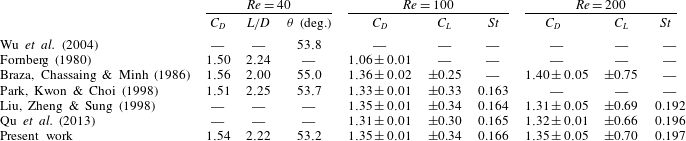
3.4 Validation
The computation results are validated using the results of 2D flow over a stationary circular cylinder at
 $Re=40$
,
 $100$
and
 $200$
. The left side of table 1 presents drag coefficients, reattachment lengths (
 $L/D$
) and separation angles (
 $\unicode[STIX]{x1D703}$
) for the present calculation at
 $Re=40$
compared with values from the literature, and the right side of table 1 shows drag and lift coefficients (
 $C_{D}$
and
 $C_{L}$
, respectively) and Strouhal number (
 $St=f_{St}D/U_{0}$
) for comparison at
 $Re=100$
and
 $200$
. The formulae of
 $C_{D}$
and
 $C_{L}$
are given in appendix B. Note that
 $C_{D}$
and
 $C_{L}$
are represented as
 $a\pm b$
with a mean value of
 $a$
and a maximum deviation of
 $b$
. The present calculation accurately predicts steady and unsteady characteristics, such as shedding frequency and the oscillations of drag and lift coefficients for
 $Re=40$
,
 $100$
and
 $200$
.
Drag coefficients, lift coefficients and Strouhal number for flow over a stationary circular cylinder at different Reynolds numbers.
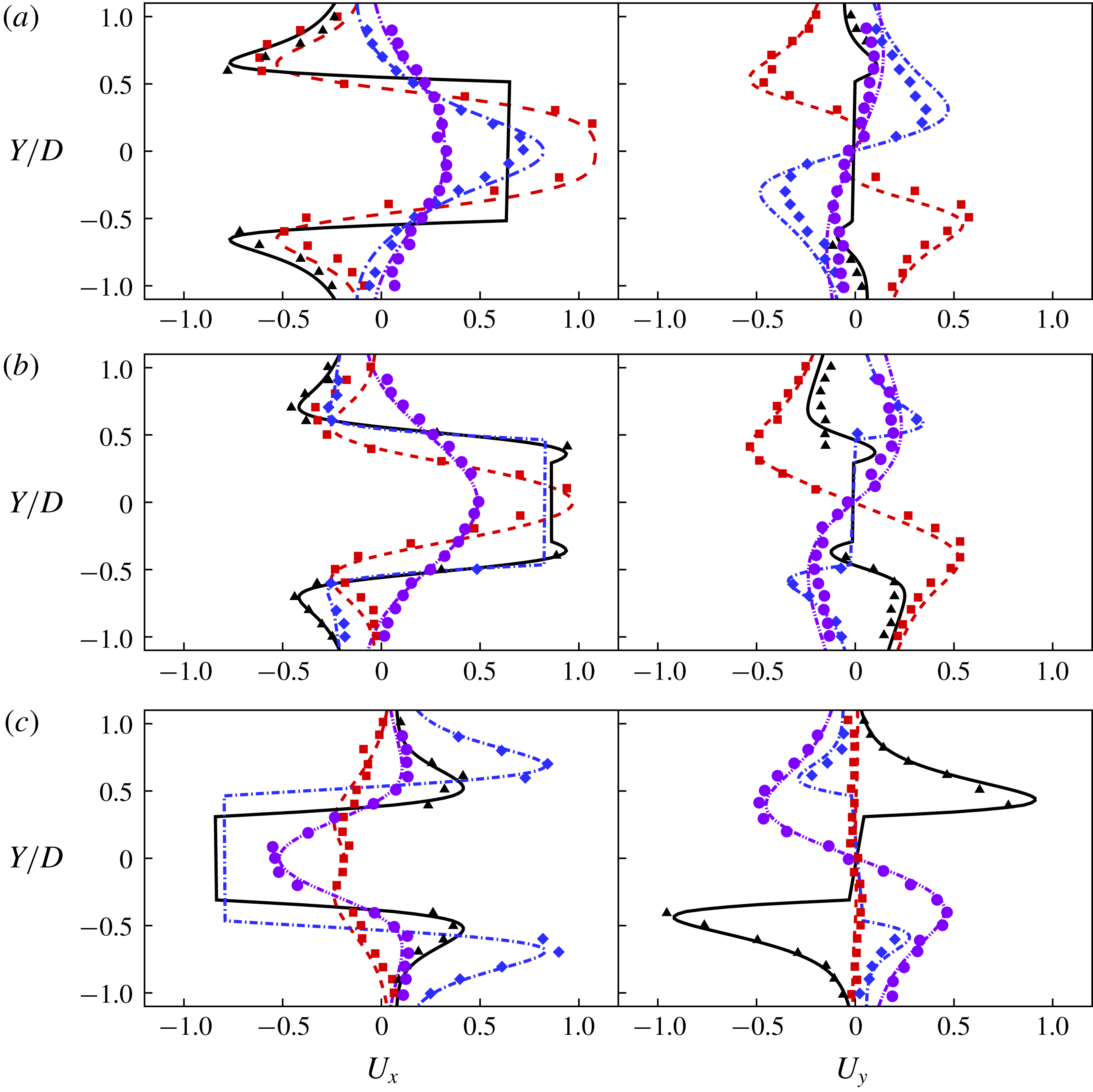
Velocity profiles along the
 $X$
direction for different cylinder phases of (a)
 $\unicode[STIX]{x1D719}=180^{\circ }$
, (b)
 $\unicode[STIX]{x1D719}=210^{\circ }$
and (c)
 $\unicode[STIX]{x1D719}=330^{\circ }$
at
 $X$
locations of
 $X/D=-0.6$
(red),
 $0.0$
(black),
 $0.6$
(blue) and
 $1.2$
(violet), where
 $X$
and
 $Y$
represent the transverse and streamwise components of the inertial coordinate (
 $\boldsymbol{X}$
), respectively. Solid curves show the present velocity results, while the experimental results of Dütsch et al. (Reference Dütsch, Durst, Becker and Lienhart1998) are marked as symbols.
Drag coefficient with time variation for the oscillating cylinder. The curve and various symbols represent the present numerical results and the experimental results of Dütsch et al. (Reference Dütsch, Durst, Becker and Lienhart1998), respectively.

Next, an oscillating cylinder in a fluid at rest is considered for validating the present calculation for a moving cylinder. The two characteristic parameters are chosen as the Reynolds number,
 $Re$
, which is
 $100$
, and the Keulegan–Carpenter number,
 $KC$
, which is
 $5$
, in order to compare the present results with the experimental data of Dütsch et al. (Reference Dütsch, Durst, Becker and Lienhart1998). The translational motion
 $X(t)$
is given by
 $X(t)=A\sin (2\unicode[STIX]{x03C0}f_{d}t)$
. Here, the Reynolds number is defined as
 $Re=U_{max}D/\unicode[STIX]{x1D708}$
, where
 $U_{max}=2\unicode[STIX]{x03C0}f_{d}A$
is the maximum velocity of the cylinder, and
 $KC$
is defined as
 $KC=U_{max}/(f_{d}D)$
, where
 $f_{d}$
is the oscillation driving frequency. Figure 2 shows streamwise (
 $U_{x}$
) and transverse (
 $U_{y}$
) velocity profiles along the direction for three different cylinder phases (
 $\unicode[STIX]{x1D719}=180^{\circ }$
,
 $210^{\circ }$
and
 $330^{\circ }$
) at
 $X$
locations (
 $X/D=-0.6$
,
 $0.0$
,
 $0.6$
and
 $1.2$
), where
 $\unicode[STIX]{x1D719}$
is represented as
 $0\leqslant \unicode[STIX]{x1D719}(t)=2\unicode[STIX]{x03C0}f_{d}(t-t_{0})\leqslant 2\unicode[STIX]{x03C0}$
. Note that
 $t_{0}$
represents an offset time used to set when the centre of the cylinder is located at
 $x_{cyl}=0$
. Figure 3 shows a comparison of time variations of the drag coefficient for an oscillating cylinder in a fluid at rest with those reported by Dütsch et al. (Reference Dütsch, Durst, Becker and Lienhart1998). Overall, the present numerical results are in good agreement with those of Dütsch et al. (Reference Dütsch, Durst, Becker and Lienhart1998) although the local extremum is slightly underpredicted compared to the corresponding values of Dütsch et al. (Reference Dütsch, Durst, Becker and Lienhart1998).
Comparison of flow patterns obtained from the present study (a,c) with those from Al-Mdallal et al. (Reference Al-Mdallal, Lawrence and Kocabiyik2007) (b,d) for a streamwise oscillatory cylinder at
 $Re=200$
. The oscillation conditions are
 $A/D=0.1,~f_{d}/f_{St}=1.95$
for (a,b) and
 $A/D=0.3,~f_{d}/f_{St}=2.0$
for (c,d), respectively.

We have performed numerical simulations of flow over a streamwise oscillating cylinder at
 $Re=200$
, considering two oscillation conditions (
 $A/D=0.1,~f_{d}/f_{St}=1.95$
and
 $A/D=0.3,~f_{d}/f_{St}=2.0$
) at
 $Re=200$
, under which the corresponding flow patterns show subharmonic lock-in and symmetric harmonic lock-in regions, respectively. Figure 4 indicates that the present results show qualitatively good agreement with those of Al-Mdallal et al. (Reference Al-Mdallal, Lawrence and Kocabiyik2007).
Comparison of the present results for (a) the mean drag coefficient and (b) r.m.s. lift coefficient on the streamwise oscillating circular cylinder with different driving amplitudes
 $A/D$
and
 $f_{d}/f_{St}=1$
at
 $Re=175$
with those of Leontini et al. (Reference Leontini, Jacono and Thompson2013).
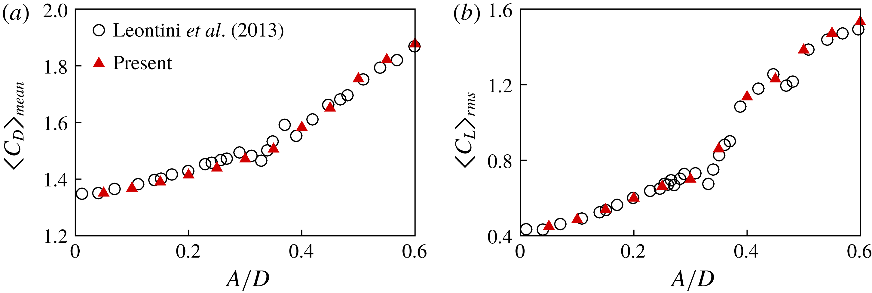
The present numerical method is validated by carrying out simulations of flow over a streamwise oscillating circular cylinder, by referring to the results of Leontini et al. (Reference Leontini, Jacono and Thompson2013) at
 $Re=175$
. Figure 5(a,b) shows the mean of drag coefficient
 $\langle C_{D}\rangle _{mean}$
, and r.m.s. of lift coefficient
 $\langle C_{L}\rangle _{rms}$
, for various driving amplitudes at the fixed driving frequency of
 $f_{d}/f_{St}=1$
, respectively. The results obtained from the present simulations are in good agreement with those of Leontini et al. (Reference Leontini, Jacono and Thompson2013), which confirms that the present method provides accurate predictions of the aerodynamic forces acting on a moving cylinder.
4 Results
4.1 Lock-in region
The majority of previous studies on flows over oscillating cylinders have investigated the lock-in phenomenon. For transverse oscillations, Bishop & Hassan (Reference Bishop and Hassan1964) reported a lock-in phenomenon in which the system of the cylinder and its wake became synchronized at the driving frequency of the cylinder only. In this case, the lock-in signals of the lift coefficient are sinusoidal, and corresponding spectra are composed of a peak. In the case of a cylinder oscillating streamwise, on the other hand, Karanth, Rankin & Sridhar (Reference Karanth, Rankin and Sridhar1995) observed a non-sinusoidal lift coefficient even in lock-in. Cetiner & Rockwell (Reference Cetiner and Rockwell2001) and Al-Mdallal et al. (Reference Al-Mdallal, Lawrence and Kocabiyik2007) used Lissajous patterns of lift-coefficient history to analyse the lock-in phenomenon, and Leontini et al. (Reference Leontini, Jacono and Thompson2011, Reference Leontini, Jacono and Thompson2013) used primary frequency and Poincaré sections for analysing the lock-in phenomenon. In this study, lock-in phenomena are analysed using the spectra of lift coefficients in which spectral peaks sharply converged to frequencies that are explicit in the driving frequency,
 $f_{d}$
.
Time history of the lift coefficient: (a)
 $A/D=0.85$
and
 $f_{d}/f_{St}=2.1$
, and (b)
 $A/D=0.85$
and
 $f_{d}/f_{St}=2.0$
. These show an example of the comparison between histories of short-time and long-time initial transition lift coefficients. The lift coefficient after initial transient periods: (c) and (d) for (a) and (b), respectively.
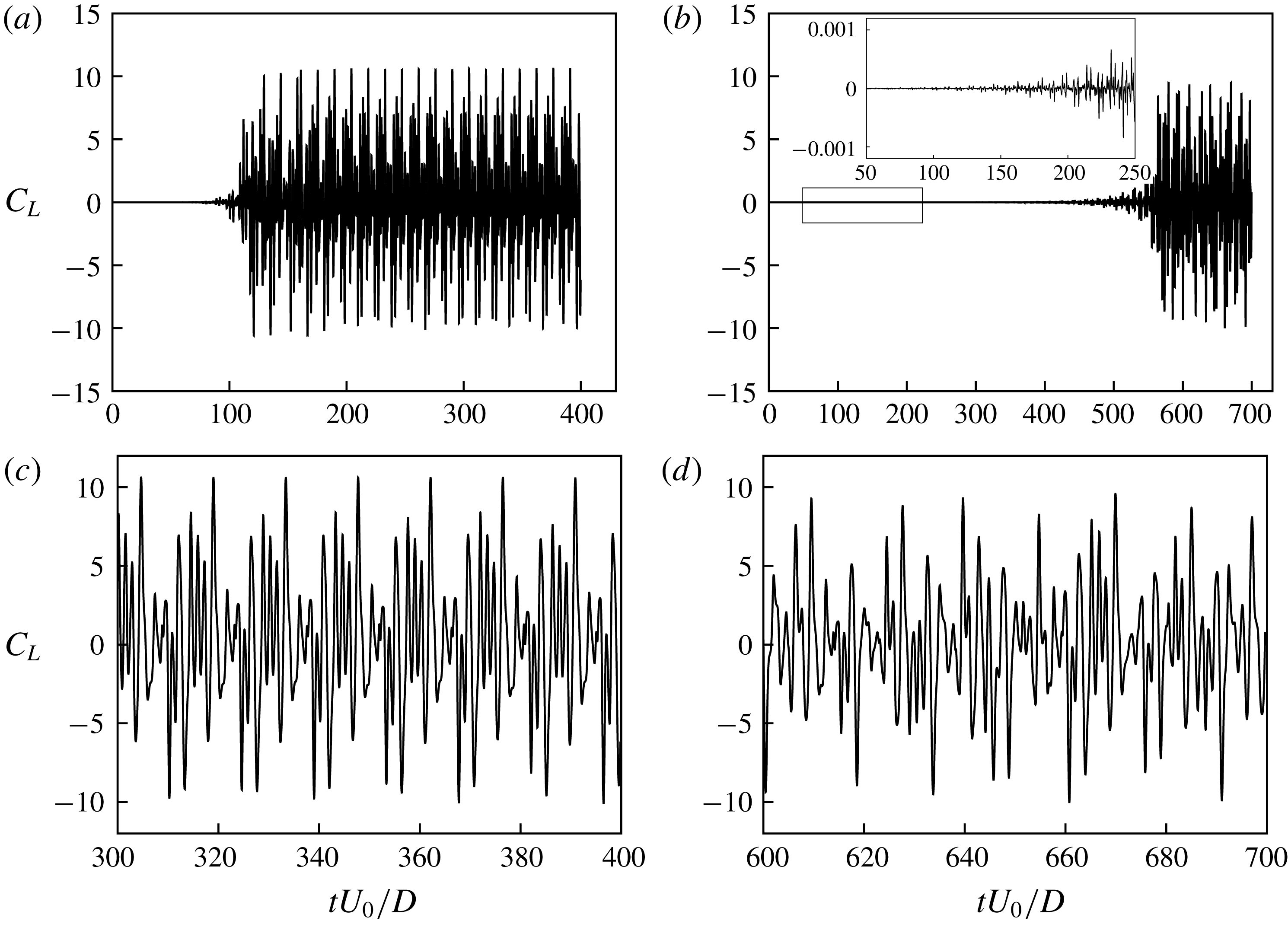
Before proceeding further with the spectral analysis, we first investigate temporal oscillation patterns of the lift coefficient for the streamwise oscillating cylinder. The lift coefficient in figure 6(a) shows a predominant mode with very low amplitude after a short-time initial transition. From figure 6(c), a large amplitude of lift oscillations is observed in the predominant mode after the initial transition. In contrast, figure 6(b) shows a lift coefficient with a low amplitude in a long-time initial transition (see the inset of figure 6
b), whereas the predominant mode after the transition has a lift coefficient with a high amplitude in figure 6(d). Note that the transition time in figure 6(b) is more than four times longer than that in figure 6(a). The long-time initial transition at the same oscillation condition was observed in several previous studies, which is called a mode competition. Ongoren & Rockwell (Reference Ongoren and Rockwell1988) and Konstantinidis, Balabani & Yianneskis (Reference Konstantinidis, Balabani and Yianneskis2007) reported vortex shedding mode competition, which involves competition between symmetrical and antisymmetrical vortex shedding modes. Cetiner & Rockwell (Reference Cetiner and Rockwell2001) found the generation of mode competition by observing the time history of the lift coefficient at
 $f_{d}/f_{0}=1$
, which was related to a process of nonlinear bifurcation that yields two branches of solutions. In this study, lock-in phenomena are analysed after lift coefficients reach their predominant modes.
Spectra showing time histories of the lift coefficient: (a) non-lock-in case (low frequency) with
 $A/D=0.8$
and
 $f_{d}/f_{St}=0.5$
; (b) non-lock-in case (high frequency) with
 $A/D=0.8$
and
 $f_{d}/f_{St}=2.5$
; (c) subharmonic lock-in case with
 $A/D=0.8$
and
 $f_{d}/f_{St}=1.2$
; (d) harmonic lock-in case with
 $A/D=0.8$
and
 $f_{d}/f_{St}=0.8$
.
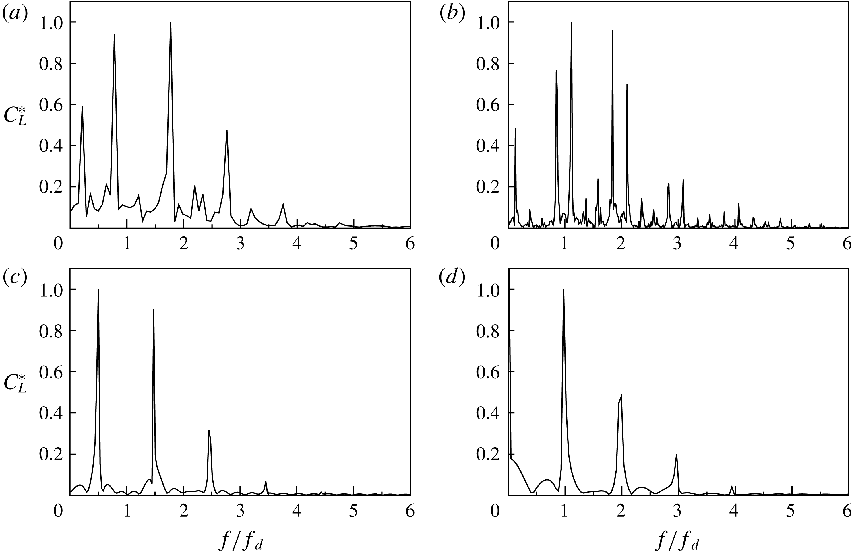
Figure 7 represents the spectra of lift coefficients. The
 $x$
-axis (
 $f/f_{d}$
) is the spectrum frequency normalized by the driving frequency, and the
 $y$
-axis (
 $C_{L}^{\ast }$
) is the spectrum density of the lift coefficient, which is normalized by its maximum peak value. Figure 7(a,b) shows that the spectral peaks are observed in the frequency where it is not related to the driving frequency. Figure 7(c,d), on the other hand, shows that the spectral peaks sharply converge to the driving frequency, indicating that the frequency components of the lift coefficient are represented without the natural Strouhal frequency. In this study, these phenomena are defined as lock-in. Furthermore, Figure 7(c,d) illustrates that there are two different kinds of features in lock-in phenomena: (c) one is that the spectral peaks are at
 $f/f_{d}=1/2+n$
, and (d) the other is the occurrence of peaks at
 $f/f_{d}=1+n$
, where
 $n=0,1,2,\ldots ,\infty$
. These are classified as (c) subharmonic lock-in and (d) harmonic lock-in, respectively.
Lissajous patterns: (a) non-lock-in case (low frequency) with
 $A/D=0.8$
and
 $f/f_{d}=0.5$
; (b) non-lock-in case (high frequency) with
 $A/D=0.8$
and
 $f/f_{d}=2.5$
; (c) subharmonic lock-in case with
 $A/D=0.8$
and
 $f/f_{d}=1.2$
; (d) harmonic lock-in case with
 $A/D=0.8$
and
 $f/f_{d}=0.8$
.
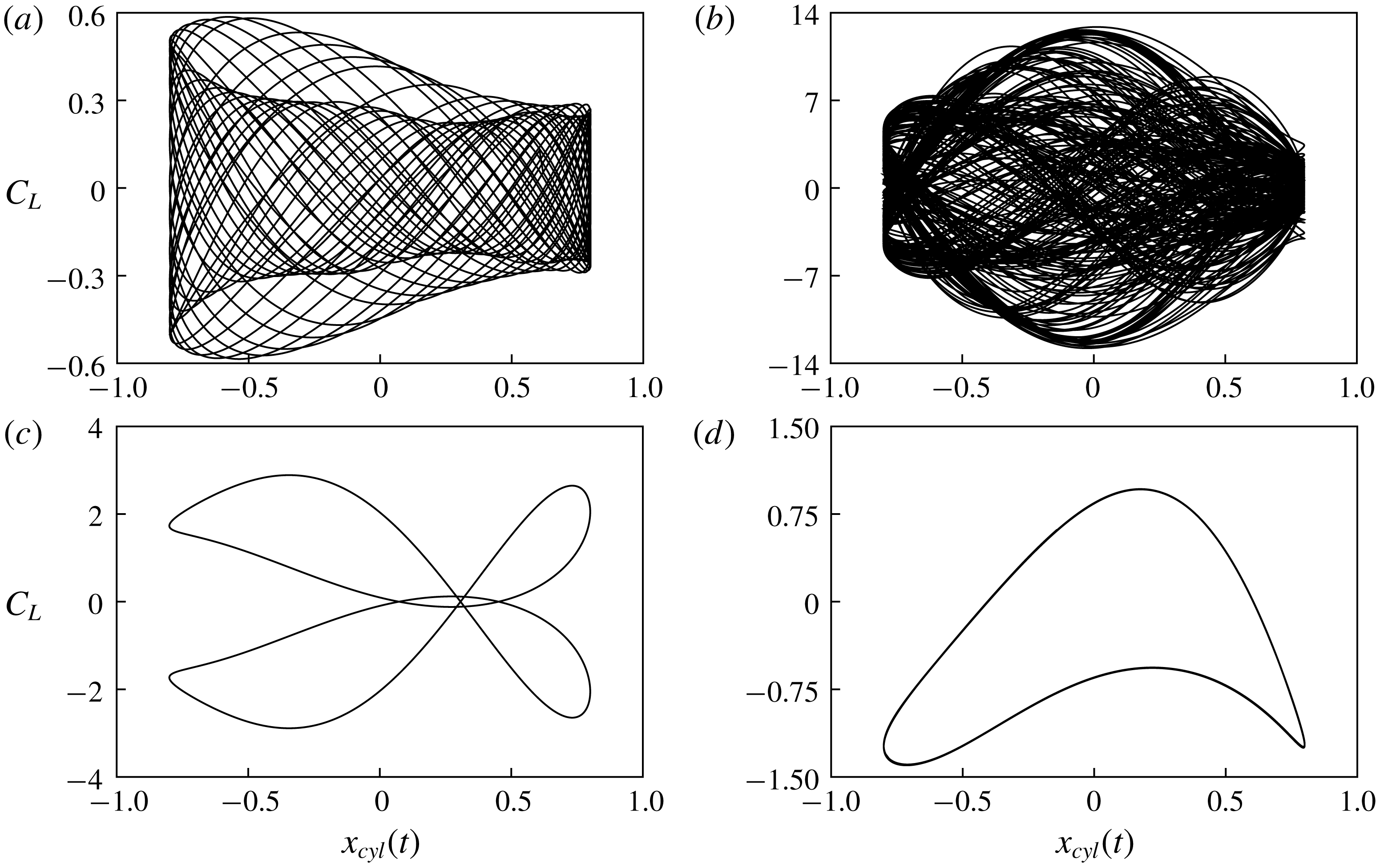
Figure 8 shows Lissajous patterns for different driving frequencies
 $f_{d}/f_{St}=0.5,~2.5,~1.2$
, and
 $0.8$
with the driving amplitude
 $A/D=0.8$
. Note that the four cases are the same as in figure 7 for lock-in classification with spectral density analysis. The Lissajous patterns in figure 8(a,b) show that the phases are unlocked; where the cases are classified as being in non-lock-in mode on the basis of the spectral density analysis. In contrast, a phase lock is clearly observed in the Lissajous patterns, as shown in figure 8(c,d), where the cases (c) and (d) are classified as demonstrating subharmonic lock-in and harmonic lock-in, respectively. This confirms that the lock-in classification based on the spectral density analysis is consistent with that from Lissajous patterns.
Frequency content of the lift force signal as a function of
 $f_{d}$
at
 $A/D=0.4$
. The greyscale contour plot represents the spectrum amplitude
 $(C_{L}^{\ast })$
, while the line plot indicates
 $C_{L}^{\ast }$
at
 $f_{d}/f_{St}=1.5$
.
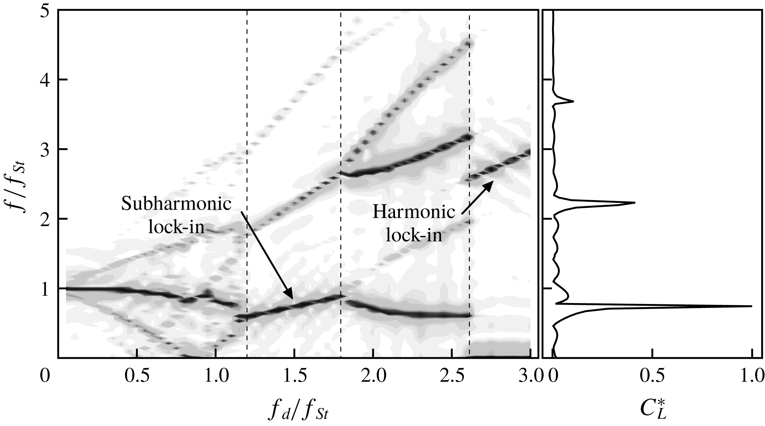
The spectra of lift coefficients show that lock-in phenomena are distributed over a range of driving frequencies and amplitudes, which is called the lock-in region. Leontini et al. (Reference Leontini, Jacono and Thompson2011) presented the variation of the frequency content of the lift force with respect to the driving amplitude, which indicates that the spectral peaks are sharply converged when the cylinder oscillates with a certain driving amplitude range and that these series of frequency peaks are located at the driving frequency. In the present study, figure 9 shows the change of the spectrum of lift force with respect to the driving frequency. The
 $y$
-axis of the figure represents the spectrum frequency normalized by the Strouhal frequency, and the
 $x$
-axis represents the driving frequency. The magnitude of the spectra is represented in greyscale, and the spectral peaks appear as dark-grey curves. There are two separate regions where the spectral peaks are sharply converged to the frequency; these are shown as linear regions with respect to the driving frequency. Furthermore, these two regions have different slopes for linear peak lines. The line in the high-frequency region, which involves harmonic lock-in, are steeper than those in other regions, which are subharmonic. It is proposed that there are different kinds of lock-in regions, i.e. subharmonic lock-in regions and harmonic lock-in regions, which are characterized by the positions of the spectral peaks.
Lock-in region map showing the driving amplitude versus the driving frequency at
 $Re=100$
. Subharmonic and harmonic lock-in cases are marked by circles and triangles, respectively. In addition, green and blue colours indicate non-symmetric and symmetric vortex shedding cases, respectively. Ambiguous lock-in regions are marked by grey-coloured squares. The black curves represent
 $U_{cyl}/U_{0}=1.0,~1.5$
, and
 $2.5$
. The violet curve indicates the lower bound of the driving amplitude at a given frequency for lock-in in Leontini et al. (Reference Leontini, Jacono and Thompson2013).
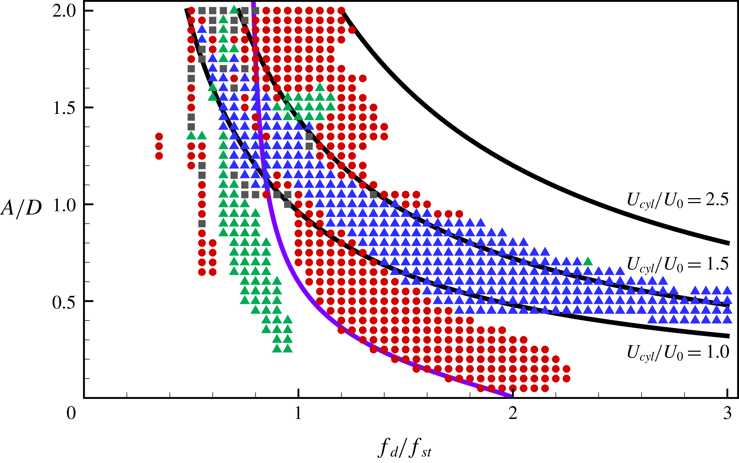
The lock-in regions with respect to various driving amplitudes and frequencies at
 $Re=100$
are presented as a map in figure 10. The
 $x$
- and
 $y$
-axes represent driving frequency and amplitude, respectively. The axes are normalized by the Strouhal frequency and the diameter of the cylinder, respectively. The driving frequency was changed from
 $f_{d}/f_{St}=0.05$
to
 $3.0$
, and the driving amplitude was changed from
 $A/D=0.05$
to
 $2.0$
with an interval of
 $0.05$
. The oscillation cases that show lock-in behaviour are marked on the map as symbols: circles for subharmonic lock-in and triangles for harmonic lock-in. Driving forces acting on the cylinder with large amplitude and frequency induce the chaotic wake patterns behind the cylinder. Owing to highly irregular wake patterns, the two-dimensional flow assumption cannot hold for strong oscillation cases with a large amplitude and high frequency. In addition, simulations of such cases require a much smaller time step to avoid numerical instability, leading to a huge computational cost. Therefore, simulation cases having
 $U_{cyl}/U_{0}\leqslant 2.5$
are considered in the present study.
The lower boundary of the subharmonic lock-in region is found at a larger driving amplitude when the driving frequency is shifted to a lower frequency from
 $f_{d}/f_{St}=2$
. This feature of lock-in threshold amplitude was observed in previous studies (Griffin & Ramberg Reference Griffin and Ramberg1976; Hall & Griffin Reference Hall and Griffin1993; Konstantinidis, Balabani & Yianneskis Reference Konstantinidis, Balabani and Yianneskis2003). Leontini et al. (Reference Leontini, Jacono and Thompson2013) observed quasi-periodicity (QP) in the non-lock-in region and modelled the vortex shedding frequency (
 $f_{s}$
) by a power law of the driving amplitude with computational data. Further, they proposed a threshold amplitude parametrized by the driving frequency (
 $f_{d}$
), where the vortex completed its own period during two cycles of the cylinder, by using the relation between
 $f_{d}$
and
 $f_{s}$
in the lock-in region. It is worth noting that the lower boundary of the subharmonic lock-in region observed in this study coincides with the threshold amplitude (Leontini et al.
Reference Leontini, Jacono and Thompson2013) marked on the map as a solid line. The upper boundary of the subharmonic region is found at a lower driving frequency for a moderate driving amplitude
 $(0.3\leqslant A/D\leqslant 1)$
as the amplitude increases. However, the upper boundary shifts towards a higher driving frequency only when the cylinder oscillates with a small driving amplitude
 $(A/D\leqslant 0.3)$
. The characteristics of the upper boundary for a small driving amplitude were also found in Griffin & Ramberg (Reference Griffin and Ramberg1976) and Al-Mdallal et al. (Reference Al-Mdallal, Lawrence and Kocabiyik2007). For a large driving amplitude
 $(A/D\geqslant 1)$
, the subharmonic region exists when
 $f_{d}/f_{St}\leqslant 1.5$
. The lower boundary of the subharmonic region seems to follow the curve of
 $U_{cyl}/U_{0}=1.5$
for a large driving amplitude.
The harmonic region marked with blue triangles on the map is a noticeable region called the symmetric harmonic region, where the flow shows symmetric vortex shedding. This has been observed in various previous studies (Ongoren & Rockwell Reference Ongoren and Rockwell1988; Konstantinidis, Balabani & Yianneskis Reference Konstantinidis, Balabani and Yianneskis2005; Nishihara, Kaneko & Watanabe Reference Nishihara, Kaneko and Watanabe2005). Interestingly, the symmetric harmonic region is located between two black curves that represent
 $U_{cyl}/U_{0}=1$
and
 $1.5$
. It is observed that a pair of counter-rotating vortices are symmetrically formed behind the cylinder moving upstream, while the strength of the vortices is weakened and no additional vortices are formed behind the cylinder moving downstream. This may be explained by the fact that a low relative speed of the cylinder moving downstream weakens inertial effects on flows behind the cylinder, which enhances the symmetric pattern of the vortices.
The harmonic lock-in region having an asymmetric vortex shedding, the so-called non-symmetric harmonic region, is marked by green triangles on the map. This region is found at
 $0.6\leqslant f_{d}/f_{St}\leqslant 1$
for a moderate driving amplitude, and at approximately
 $f_{d}/f_{St}=1$
for a large driving amplitude
 $(A/D\approx 1.5)$
. Similar to Leontini et al. (Reference Leontini, Jacono and Thompson2013), it is observed that the upper and lower vortices behind the oscillating cylinder are asymmetric and imbalanced.
4.2 Flow structures and aerodynamic coefficients
Time histories of lift coefficient and cylinder position, and snapshots of vorticity for each region during two periods of cylinder motion at
 $Re=100$
, where
 $t^{+}=(t-t_{0})U_{0}/D$
, and
 $t_{0}$
represents an offset time. (a) Subharmonic lock-in region
 $(A/D=0.4,~f_{d}/f_{St}=1.5)$
; (b) non-symmetric harmonic lock-in region
 $(A/D=0.4,~f_{d}/f_{St}=0.8)$
; (c) symmetric harmonic lock-in region
 $(A/D=0.4,~f_{d}/f_{St}=2.8)$
; (d) non-lock-in region
 $(A/D=0.4,~f_{d}/f_{St}=1.9)$
; and (e) non-lock-in region
 $(A/D=0.9,~f_{d}/f_{St}=2.4)$
. Solid and dashed lines represent anticlockwise and clockwise rotating vorticity, respectively. The minimum and maximum values of contour lines are
 $-5$
and
 $+5$
, respectively, with 20 levels.
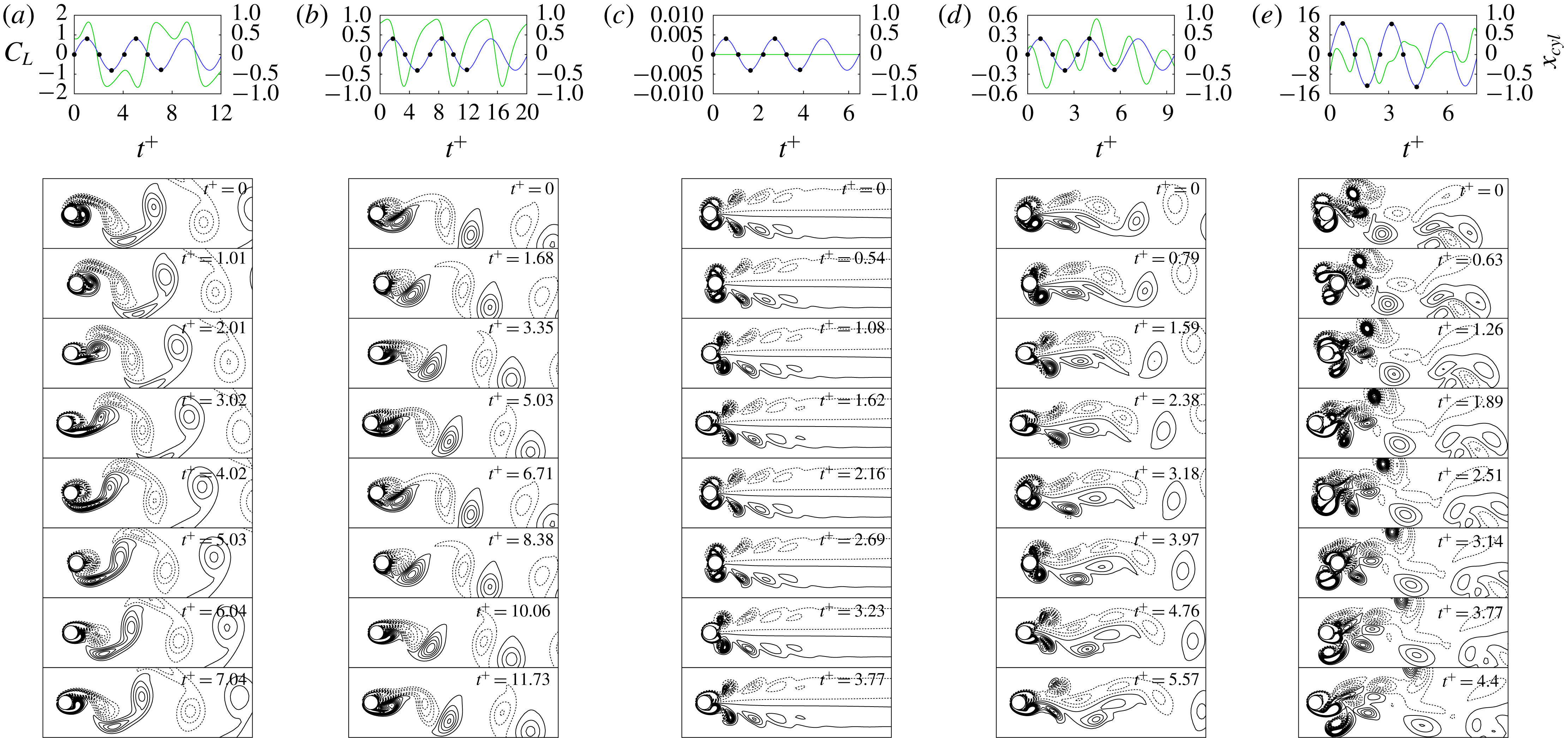
The wake patterns induced by the oscillating cylinder under various conditions of driving amplitude and frequency are classified according to the distinct regions. Figure 11 shows snapshots of the vorticity contour during two periods of cylinder oscillation, at quarter-period intervals, along with time histories of the lift coefficient with the cylinder position, where
 $t^{+}=(t-t_{0})U_{0}/D$
. Note that
 $t_{0}$
is an offset time used to define the time at which the centre of the cylinder is located at
 $x_{cyl}=0$
after wake flows become quasi-periodic. The snapshots represent the wake patterns of the subharmonic lock-in region (a), two harmonic lock-in regions (b) and (c), and non-lock-in regions (d) and (e).
Flow structures for the subharmonic lock-in case are shown in figure 11(a). The cylinder moving downstream (
 $t^{+}=0{-}2.01$
) induces an anticlockwise (ACW) rotating vortex behind the cylinder. When the cylinder moves upstream (
 $t^{+}=1.01{-}3.02$
), the vortex is convected downstream, and another ACW rotating vortex is formed behind the cylinder. At the end of the first oscillation period of the cylinder (
 $t^{+}=4.02$
), two vortices are merged and start to detach from the cylinder (
 $t^{+}=5.03$
). In the second period (
 $t^{+}=4.02{-}7.04$
), clockwise (CW) rotating vortices are formed behind the cylinder, convected downstream, and merged before detaching from the cylinder, similar to the behaviour of flow structures in the first period. These alternating CW and ACW rotating vortex-shedding patterns were frequently reported by previous studies (Griffin & Ramberg Reference Griffin and Ramberg1976; Ongoren & Rockwell Reference Ongoren and Rockwell1988; Al-Mdallal et al.
Reference Al-Mdallal, Lawrence and Kocabiyik2007; Perdikaris, Kaiktsis & Triantafyllou Reference Perdikaris, Kaiktsis and Triantafyllou2009; Leontini et al.
Reference Leontini, Jacono and Thompson2013). The vortex shedding in subharmonic regions is synchronized with two cycles of cylinder motion (Ongoren & Rockwell Reference Ongoren and Rockwell1988; Al-Mdallal et al.
Reference Al-Mdallal, Lawrence and Kocabiyik2007; Perdikaris et al.
Reference Perdikaris, Kaiktsis and Triantafyllou2009). The lift coefficient has a positive or negative peak when the cylinder motion changes from the upstream to downstream direction and vice versa (
 $t^{+}=1.01,~3.02,~5.03$
and
 $7.04$
). The lift coefficient is negative in the first period, in which the cylinder moved from the zero position to the upstream (
 $t^{+}=2.01$
), and it becomes positive in the next period (
 $t^{+}=6.04$
). This confirms that the lift coefficient is synchronized with two cycles of cylinder motion, similar to the vortex shedding.
Figure 11(b) shows the behaviour of wake flows in the non-symmetric harmonic region. A CW rotating vortex is formed behind the cylinder moving downstream (
 $t^{+}=0$
), and it pushes an existing ACW rotating vortex downstream (
 $t^{+}=1.68$
). When the cylinder moves upstream (
 $t^{+}=3.35$
), the pair of counter-rotating vortices is convected further downstream, and another pair of counter-rotating vortices is newly formed behind the cylinder (
 $t^{+}=5.03$
). As the cylinder moves downstream (
 $t^{+}=6.71$
), the new ACW rotating vortex remains near the cylinder, while the CW rotating vortex starts to detach from the cylinder. Within a cycle of the cylinder oscillation, the dynamic pattern of the vortices is completed in the non-symmetric harmonic case. It should be noted that counter-rotating vortices are not symmetrically formed behind the cylinder and the convective direction of the vortex pair is not aligned with the horizontal centreline. Similar to the flow pattern, the lift coefficient is also completed within one cycle of the cylinder oscillation. While the cylinder is moving upstream, the lift coefficient is reduced from the maximum value to the minimum value (
 $t^{+}=1.68{-}6.71$
) and then back to a positive value (
 $t^{+}=6.71{-}8.38$
). As the cylinder moves downstream (
 $t^{+}=8.38{-}11.73$
), the lift coefficient continues to increase while maintaining a positive value. Therefore, the negative and positive lift coefficients are imbalanced during one cycle of the cylinder oscillation, leading to a non-zero mean lift coefficient. This is mainly due to non-symmetric counter-rotating vortices. Similar vortex patterns were reported in Leontini et al. (Reference Leontini, Jacono and Thompson2013), where the oscillation case was
 $A/D=0.4,~f_{d}/f_{St}=0.8$
at
 $Re=175$
.
Figure 11(c) shows a symmetric vortex pattern in the symmetric harmonic region, which was observed in previous studies (Ongoren & Rockwell Reference Ongoren and Rockwell1988; Kim et al.
Reference Kim, Yoo and Sung2006; Konstantinidis & Balabani Reference Konstantinidis and Balabani2007a
; Marzouk & Nayfeh Reference Marzouk and Nayfeh2009; Feng & Wang Reference Feng and Wang2010; Leontini et al.
Reference Leontini, Jacono and Thompson2013; Konstantinidis & Bouris Reference Konstantinidis and Bouris2016). As the cylinder moves downstream (
 $t^{+}=0{-}0.54$
), two pairs of vortices are formed near the cylinder, where CW and ACW rotating vortices are dominant above and below the cylinder, respectively. The cylinder moving upstream (
 $t^{+}=1.08$
) pushes the two pairs of vortices downstream, while ACW and CW rotating vortices are weakened and disappear above and below the horizontal centreline, respectively. Moreover, the upper CW and lower ACW rotating vortices are eventually detached from the cylinder while keeping the symmetric pattern (
 $t^{+}=1.62$
). As time progresses, two pairs of vortices are newly formed immediately above and below the cylinder (
 $t^{+}=2.16$
). One cycle of vortex shedding is completed in a period of cylinder oscillation in the symmetric harmonic region. The symmetric vortex shedding is maintained during the entire oscillation period, which leads to a lift coefficient of zero.
Figure 11(d) shows flow patterns in the non-lock-in region. When the cylinder moves downstream (
 $t^{+}=0{-}0.79$
), there are two strong slightly asymmetric vortices that are CW and ACW rotating vortices above and below the cylinder, respectively, unlike those in the harmonic lock-in region. As the cylinder moves upstream (
 $t^{+}=1.59$
), the two vortices are convected downstream and become more asymmetric. Two elongated large counter-rotating vortices are found near the wake region, while alternating CW and ACW rotating vortices are observed far from the wake region. The vortex shedding cycle is incomplete during two periods of cylinder oscillation in the non-lock-in region. In contrast to the temporal behaviour of the lift coefficient in lock-in cases, the phase difference between the local minimum or maximum of lift coefficients and cylinder position varies with time, and the periodicity of the lift coefficient is not observed during the two oscillation cycles of the cylinder. In the present study, a lock-in mode is classified based on the lift coefficient during two cycles of the cylinder oscillation, because the lift coefficient spectra of the subharmonic lock-in has their peaks at
 $f/f_{d}=1/2+n$
. It should be noted that the lift coefficient in a non-lock-in mode may have a larger period than two cycles of cylinder oscillation. Leontini et al. (Reference Leontini, Jacono and Thompson2011) observed a periodicity of the lift coefficient during the
 $N\leqslant 8$
cycles of cylinder oscillation using the Poincaré map.
Figure 11(e) shows disordered vortex shedding due to the cylinder oscillation with high speed, which was also observed in Perdikaris et al. (Reference Perdikaris, Kaiktsis and Triantafyllou2009) and Leontini et al. (Reference Leontini, Jacono and Thompson2011). Depending on the cylinder position, vortex shedding is observed both in front of and behind the cylinder. The vortices shedding from the front of the cylinder are convected downstream, while the other vortices that shed behind the cylinder are convected upstream. These vortices interact with the moving cylinder, leading to steep velocity gradients and a strong lift force. The disordered vortex shedding and tangled interaction between the vortices and cylinder induce a chaotic pattern of the wake flow. Fluctuations of the lift coefficient are significantly greater in this region than in other regions. The larger fluctuations may result from steeper velocity gradients on the cylinder due to a higher driving amplitude of the cylinder oscillation. Moreover, temporal variations of the lift coefficient are not correlated with the cylinder motion, similar to the disordered vortex shedding pattern.
Effects of driving amplitude (
 $A$
) and frequency (
 $f_{d}$
) on the r.m.s. of lift coefficients,
 $\langle C_{L}\rangle _{rms}$
. Variations of
 $\langle C_{L}\rangle _{rms}$
with (a)
 $A/D$
at
 $f_{d}/f_{St}=1.5$
and (b)
 $f_{d}/f_{St}$
at
 $A/D=0.4$
.
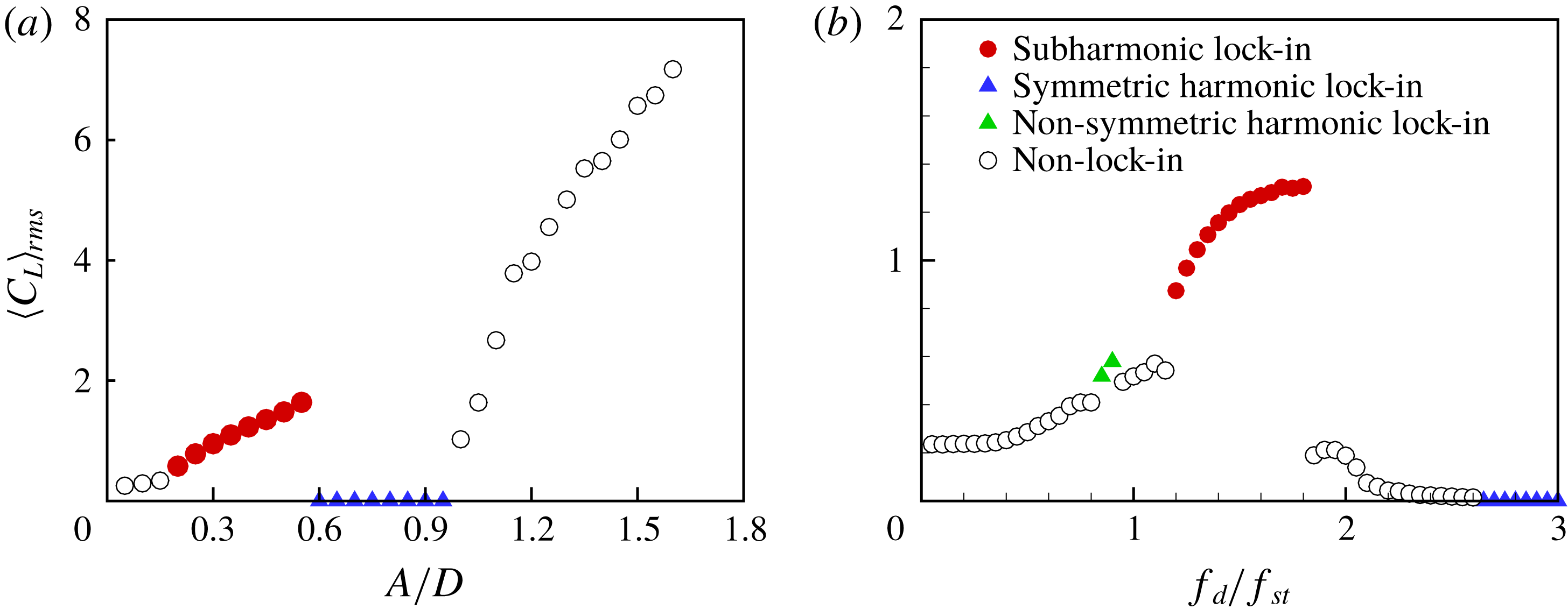
We investigate the changes of the r.m.s. value of the lift coefficient,
 $\langle C_{L}\rangle _{rms}$
, with respect to the driving amplitude and frequency in order to characterize aerodynamic features in each region. Figure 12(a) shows the effect of the driving amplitude on
 $\langle C_{L}\rangle _{rms}$
at
 $f_{d}/f_{St}=1.5$
. In the non-lock-in region with a low driving amplitude,
 $\langle C_{L}\rangle _{rms}$
increases gradually as
 $A/D$
increases. In the subharmonic lock-in region, it also appears that
 $\langle C_{L}\rangle _{rms}$
increases with
 $A/D$
, and the slope of the increment is greater than that in the non-lock-in region. For
 $0.6\leqslant A/D\leqslant 0.95$
,
 $\langle C_{L}\rangle _{rms}$
is almost zero, yielding the symmetric harmonic lock-in. As
 $A/D$
increases further,
 $\langle C_{L}\rangle _{rms}$
significantly increases with a steeper slope compared to that in the subharmonic lock-in region. The effect of driving frequency on
 $\langle C_{L}\rangle _{rms}$
at a moderate driving amplitude
 $A/D=0.4$
is also shown in figure 12(b). In the non-lock-in region,
 $\langle C_{L}\rangle _{rms}$
gradually increases as
 $f_{d}/f_{St}$
increases in
 $0<f_{d}/f_{St}<1.15$
, except for
 $f_{d}/f_{St}=0.85$
or
 $0.90$
. These exceptional cases are in the non-symmetric harmonic lock-in region, where
 $\langle C_{L}\rangle _{rms}$
is shifted slightly upwards from
 $\langle C_{L}\rangle _{rms}$
at both ends of the non-lock-in region, similar to observations in Cetiner & Rockwell (Reference Cetiner and Rockwell2001). As
 $f_{d}/f_{St}$
increases further,
 $\langle C_{L}\rangle _{rms}$
suddenly increases at
 $f_{d}/f_{St}=1.2$
and reaches its maximum at
 $f_{d}/f_{St}=1.9$
in the subharmonic lock-in region, which was also found in Marzouk & Nayfeh (Reference Marzouk and Nayfeh2009). In the non-lock-in region following the subharmonic lock-in region, the present results show that
 $\langle C_{L}\rangle _{rms}$
decreases with the increment of
 $f_{d}/f_{St}$
, as reported in Al-Mdallal et al. (Reference Al-Mdallal, Lawrence and Kocabiyik2007). For higher frequencies
 $f_{d}/f_{St}\geqslant 2.65$
,
 $\langle C_{L}\rangle _{rms}$
becomes almost zero, leading to the symmetric harmonic lock-in.
Aerodynamic force maps of an oscillating cylinder in
 $A/D{-}f_{d}/f_{St}$
space for (a)
 $\langle C_{D}\rangle _{mean}$
, (b)
 $\langle C_{D}\rangle _{rms}$
, (c)
 $|\langle C_{L}\rangle _{mean}|$
, and (d)
 $\langle C_{L}\rangle _{rms}$
values at
 $Re=100$
.
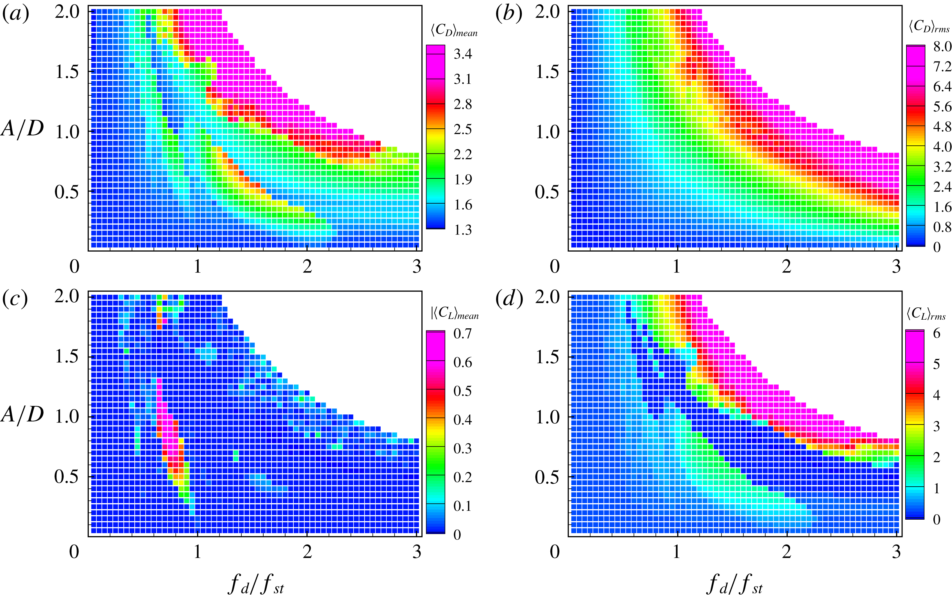
To scrutinize the effects of driving amplitude and frequency on the aerodynamic forces acting on the oscillating cylinder, we analyse time-dependent aerodynamic forces for 1820 oscillation cases after each flow reaches its predominant mode, and these are observed in terms of lock-in regions, as shown in figure 10. The contour maps in figure 13(a–d) show the mean drag coefficient
 $\langle C_{D}\rangle _{mean}$
, r.m.s. drag coefficient
 $\langle C_{D}\rangle _{rms}$
, absolute value of mean lift coefficient
 $|\langle C_{L}\rangle _{mean}|$
, and r.m.s. lift coefficient
 $\langle C_{L}\rangle _{rms}$
, respectively. Void regions in the contour plots are non-observed oscillating cases, where the driving amplitudes and frequencies are so high that the limitation on the cylinder oscillation speed,
 $U_{cyl}/U_{0}=2.5$
, is exceeded.
Figure 13(a) indicates that
 $\langle C_{D}\rangle _{mean}$
is larger in non-symmetric harmonic and subharmonic lock-in regions than in non-lock-in regions. In the non-symmetric harmonic region,
 $\langle C_{D}\rangle _{mean}$
increases with the driving amplitude, and its maximum is approximately 1.3 times larger than that in the surrounding non-lock-in case. In the subharmonic region,
 $\langle C_{D}\rangle _{mean}$
increases up to 2.5 because either the driving frequency or amplitude
 $(0.3\leqslant A/D\leqslant 1)$
increases. In a transitional region from the subharmonic lock-in region to the symmetric harmonic lock-in region,
 $\langle C_{D}\rangle _{mean}$
sharply decreases to that for the case of a non-oscillating cylinder. In the symmetric harmonic region,
 $\langle C_{D}\rangle _{mean}$
gradually increases with increments of either the driving amplitude or frequency. With a large driving amplitude and high frequency,
 $\langle C_{D}\rangle _{mean}$
in the upper non-lock-in region becomes more than three times larger than that for the non-oscillating cylinder case.
Figure 13(b) clearly shows that, in general,
 $\langle C_{D}\rangle _{rms}$
monotonically increases with both the driving amplitude and frequency, in contrast to the behaviour of
 $\langle C_{D}\rangle _{mean}$
. Furthermore,
 $\langle C_{D}\rangle _{rms}$
seems to be proportional to either the magnitude of the acceleration or velocity of cylinder motion because the oscillating motion is aligned with the flow direction, which may lead to a direct influence on variations of
 $C_{D}$
.
As expected, figure 13(c) shows that
 $\langle C_{L}\rangle _{mean}$
is nearly zero, except in the non-symmetric lock-in region, because counter-rotating vortices are symmetrically and alternately detached above and below the cylinder. However, in the non-symmetric lock-in region, counter-rotating vortices behind the cylinder introduce an imbalance between the negative and positive lift coefficients during one cycle of the cylinder oscillation, yielding a non-zero mean lift coefficient. At
 $Re=100$
, a non-zero
 $\langle C_{L}\rangle _{mean}$
is found for
 $0.6\leqslant f_{d}/f_{St}\leqslant 1$
with a moderate driving amplitude;
 $|\langle C_{L}\rangle _{mean}|$
increases up to 0.7 as the driving amplitude increases.
Figure 13(d) shows that
 $\langle C_{L}\rangle _{rms}$
ranges from
 $0.24$
to
 $0.5$
in the non-lock-in region, which is larger than
 $\langle C_{L}\rangle _{rms}=0.24$
for the non-oscillating case. In the subharmonic lock-in region,
 $\langle C_{L}\rangle _{rms}$
gradually increases from
 $0.9$
to
 $1.8$
as the driving amplitude or frequency increases, while
 $\langle C_{L}\rangle _{mean}$
is nearly zero in figure 13(c). This is due to the symmetric and alternating counter-rotating vortex pattern similar to von Kármán vortex shedding. Interestingly, the fluctuations of
 $C_{L}$
are negligible in the symmetric harmonic lock-in region, which results in
 $\langle C_{L}\rangle _{rms}\approx 0$
. This is because the vortices near the cylinder are vertically symmetric. In the non-lock-in region for
 $U_{cyl}/U_{0}\geqslant 1.5$
,
 $\langle C_{L}\rangle _{rms}$
increases up to
 $8.5$
as
 $U_{cyl}$
increases, similar to the behaviour of
 $\langle C_{D}\rangle _{mean}$
in figure 13(a).
Blackburn & Henderson (Reference Blackburn and Henderson1999) investigated energy transfers from the fluid to the cylinder, considering forced transverse oscillating circular cylinders, where the energy transfer coefficient was determined by using the lift coefficient and transverse oscillating velocity. They found passive energy transfers from the fluid to the cylinder in the lock-in region. Later, Konstantinidis & Balabani (Reference Konstantinidis and Balabani2007b ) observed inflow-perturbation-induced positive energy transfer to the stationary cylinder. Similar to the work by Blackburn & Henderson (Reference Blackburn and Henderson1999), we investigate energy transfers from the fluid to the streamwise oscillating cylinder by using the following energy coefficient:
 $$\begin{eqnarray}E=\frac{1}{T_{0}-t_{0}}\int _{t_{0}}^{T_{0}+t_{0}}C_{D}(t){\dot{x}}_{cyl}(t)\,\text{d}t,\end{eqnarray}$$
where
 ${\dot{x}}_{cyl}(t)$
is streamwise oscillating velocity,
 $t_{0}$
is an offset time used to define the time at which the centre of the cylinder is located at
 $x_{cyl}=0$
after wake flows become quasi-periodic, and
 $T_{0}$
is set to 20 periods of the cylinder oscillation,
 $T_{0}=20/(2\unicode[STIX]{x03C0}f_{d})$
.
Energy transfer coefficient map of an oscillating cylinder in
 $A/D{-}f_{d}/f_{St}$
space at
 $Re=100$
.
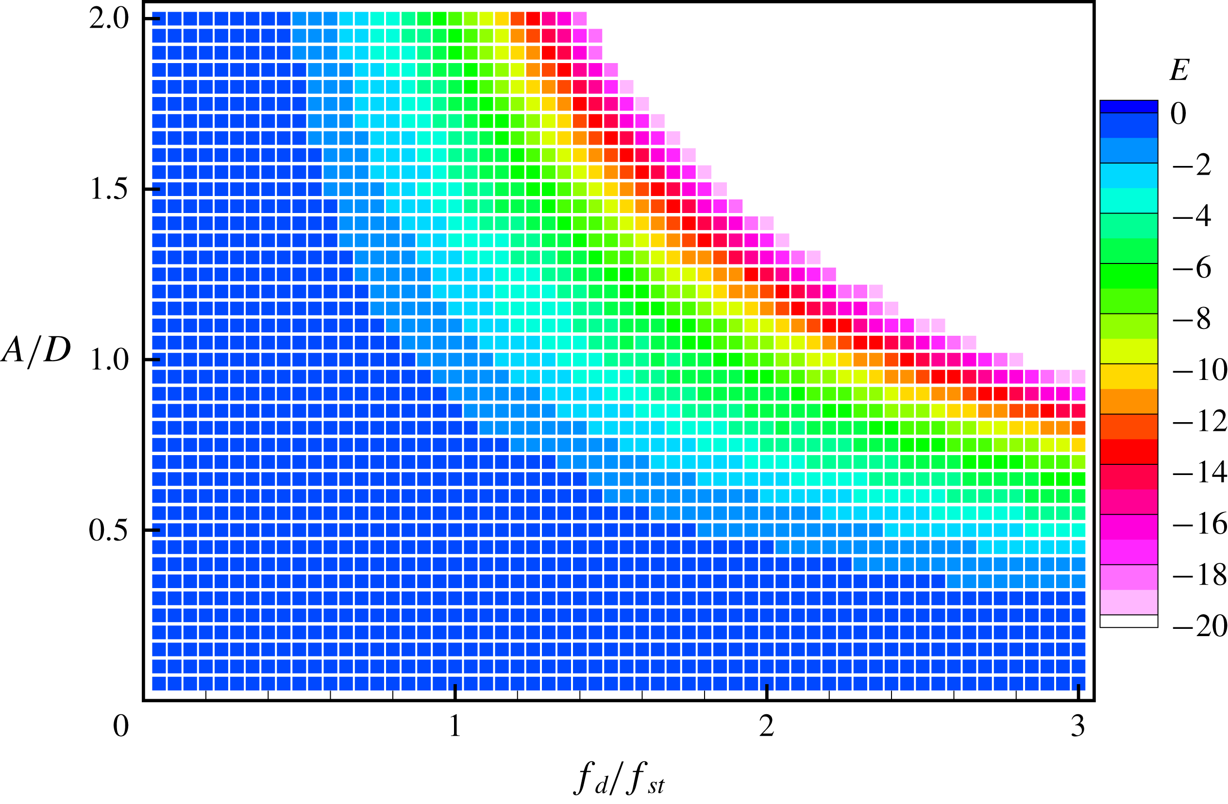
Figure 14 shows the energy coefficient
 $E$
depending on the driving amplitude and frequency at
 $Re=100$
;
 $E$
is negative for all the cases, implying that energy is transferred from the cylinder to the fluid. The absolute value of
 $E$
increases as the driving amplitude or frequency of the cylinder increase. This indicates that the stronger cylinder oscillation transfers more energy from the cylinder to the fluid. When the streamwise forced oscillating cylinder moves upstream (negative velocity), the relative velocity to the free stream increases, resulting in an increase in drag force (passive drag fluctuations). Conversely, when moving downstream (passive velocity), the relative speed to the free stream decreases, resulting in a decrease in drag force (negative drag fluctuations). Thus, the drag and velocity are mostly out of phase for a streamwise forced oscillating cylinder, which leads to
 $E\leqslant 0$
.
4.3 Reynolds-number effects
Next, we perform parametric studies at
 $Re=40$
and
 $200$
by varying the driving frequency
 $f_{d}/f_{St}$
and amplitude
 $A/D$
in order to investigate the effect of Reynolds number on the lock-in region. For each Reynolds-number case,
 $f_{d}/f_{St}$
is changed from
 $0.05$
to
 $3.0$
at intervals of 0.05, while
 $A/D$
is changed from 0.05 to 2.0. However, for the
 $Re=200$
case, simulations are restricted to the cases satisfying
 $U_{cyl}/U_{0}\leqslant 2.5$
to avoid extremely small time steps for ensuring stable computation. The lock-in regions are classified in the same manner as for the
 $Re=100$
case; peak features of the subharmonic lock-in spectrum converged to
 $f/f_{d}=0.5+n$
, while peak features of the harmonic lock-in spectrum converged to
 $f/f_{d}=1+n$
for
 $n=0,1,2,\ldots .$
Lock-in region map showing the driving amplitude versus the driving frequency at
 $Re=200$
. Lock-in regions and lines are marked in the same manner as in figure 10.
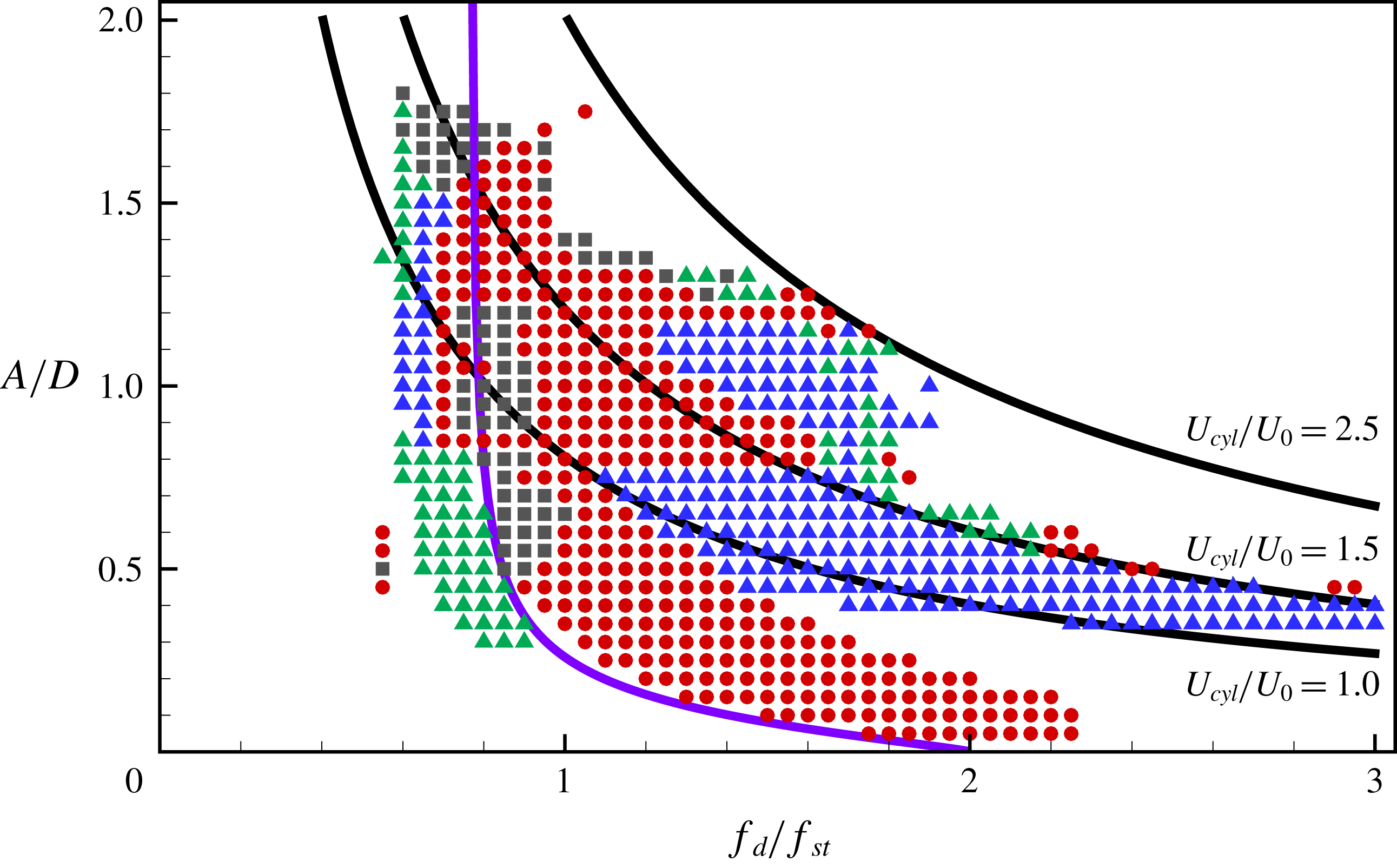
Figure 15 shows that the lower boundary of the subharmonic lock-in region of
 $Re=200$
for
 $A/D\leqslant 0.75$
is found for a larger driving amplitude when the driving frequency is shifted to a lower frequency from
 $f_{d}/f_{St}=2$
. The boundary coincides with the threshold amplitude (Leontini et al.
Reference Leontini, Jacono and Thompson2013) marked on the map as a solid line, similar to that for
 $Re=100$
in figure 10. The upper boundary of the subharmonic region is observed at a lower driving frequency for
 $0.3\leqslant A/D\leqslant 0.75$
as
 $A/D$
increases. The symmetric harmonic region is bounded by
 $1.0\leqslant U_{cyl}/U_{0}\leqslant 1.5$
with
 $A/D\leqslant 0.75$
. Similarly, such a bounded region for the symmetric harmonic lock-in is also found at
 $Re=100$
. When
 $1.0\leqslant U_{cyl}/U_{0}\leqslant 1.5$
, the subharmonic region is observed at
 $Re=200$
for
 $0.75<A/D<1.7$
, but it is not observed at
 $Re=100$
. The symmetric harmonic region is also found at
 $Re=200$
for
 $0.75<A/D<1.2$
when
 $1.5\leqslant U_{cyl}/U_{0}\leqslant 2.0$
. The non-symmetric harmonic region is found at
 $0.3\leqslant A/D\leqslant 0.8$
for a narrow driving frequency range
 $(0.6\leqslant f_{d}/f_{St}\leqslant 1)$
, which is also observed at
 $Re=100$
. In contrast to the
 $Re=100$
case, non-lock-in regions are observed for a high driving amplitude (
 $A/D>1.7$
) at
 $Re=200$
, regardless of the driving frequency.
Time histories of lift coefficient and cylinder position, and snapshots of vorticity for each region during two periods of cylinder motion at
 $Re=200$
. (a) Subharmonic lock-in region
 $(A/D=0.4,~f_{d}/f_{St}=1.2)$
; (b) non-symmetric harmonic lock-in region
 $(A/D=0.4,~f_{d}/f_{St}=0.8)$
; (c) symmetric harmonic lock-in region
 $(A/D=0.4,~f_{d}/f_{St}=2.4)$
; (d) non-lock-in region
 $(A/D=0.4,~f_{d}/f_{St}=1.6)$
; and (e) non-lock-in region
 $(A/D=0.8,~f_{d}/f_{St}=2.4)$
. Vortices are represented in the same manner as in figure 11.
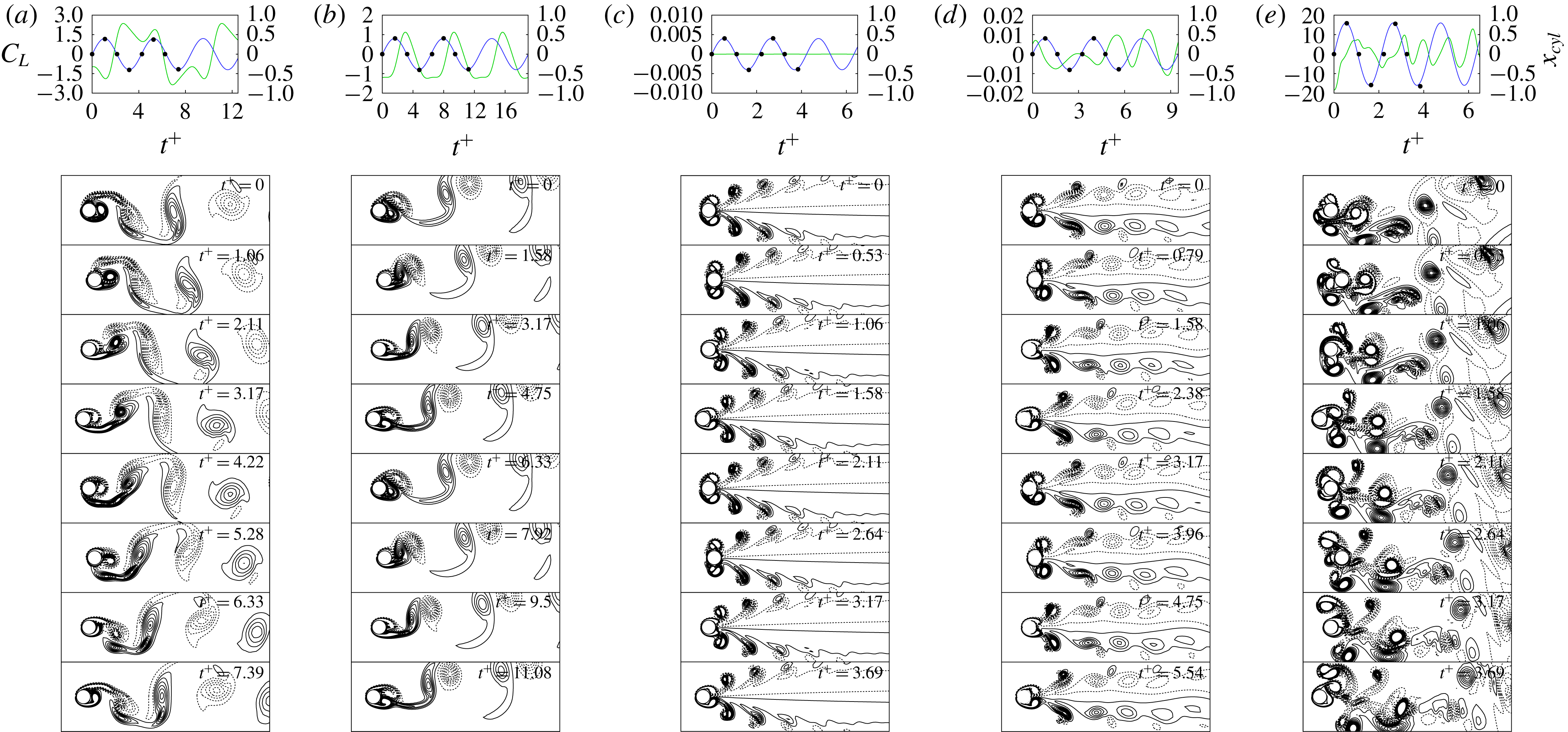
Wake patterns for each distinct region at
 $Re=200$
are presented in figure 16. The snapshots of figure 16 represent the vorticity contours during two periods of the cylinder oscillation. The wake patterns of the subharmonic lock-in region, two harmonic lock-in regions and non-lock-in regions are shown in figure 16(a–e), respectively. Figure 16(a) shows flow structures of subharmonic lock-in at
 $Re=200$
. Similar to the flow pattern for subharmonic lock-in at
 $Re=100$
, the ACW rotating vortex is located behind the cylinder when the cylinder moves downstream (
 $t^{+}=0{-}1.06$
). As the cylinder moves upstream, the ACW rotating vortex begins to be detached after the newly formed ACW rotating vortex is merged with the existing one (
 $t^{+}=1.06{-}3.17$
). However, unlike
 $Re=100$
, the ACW rotating vortex is elongated by the CW rotating vortex formed by the cylinder moving downstream in the second period (
 $t^{+}=3.17{-}5.28$
). This flow pattern completes one period for two periods of the cylinder oscillation. As in the case of the lift coefficient of subharmonic lock-in for
 $Re=100$
, the peaks of lift coefficient are observed when the motion of the cylinder changes from upstream to the downstream direction, and the lift coefficient is synchronized with two cycles of the cylinder motion. The behaviour of wake flows in the non-symmetric harmonic region at
 $Re=200$
is shown in figure 16(b), and this is very similar to that at
 $Re=100$
; that is, when the cylinder moves downstream, a pair of vortices is convected downstream, and the flow pattern of the vortices is synchronized with a cycle of cylinder motion. The ACW and CW rotating vortices formed behind the cylinder are not symmetric but are convected to a direction shifted slightly upwards, which leads to a non-zero mean lift coefficient. Figure 16(c) shows the flow patterns in the symmetric harmonic lock-in region at
 $Re=200$
. Similar to the
 $Re=100$
case, two pairs of vortices are symmetrically formed above and below the cylinder in the phase of the cylinder moving downstream (
 $t^{+}=0{-}0.53$
), while two pairs of vortices are detached in the phase of the cylinder moving upstream (
 $t^{+}=0.53{-}1.58$
). However, it should be noted that, unlike the flow patterns at
 $Re=100$
, the two counter-rotating vortices in both the upper and lower regions coexist and convect downstream while maintaining a symmetric pattern. Unlike the flow pattern of the non-lock-in at
 $Re=100$
, figure 16(d) shows the occurrence of a quite symmetric flow pattern near the region behind the cylinder even in the non-lock-in region at
 $Re=200$
. Only wake flows in the region further downstream are slightly asymmetric. As shown in the time history of lift coefficient, the vortex shedding period is incomplete during the two periods of the cylinder motion. Figure 16(e) shows flow patterns due to the cylinder vibrating with a high speed in the non-lock-in region. Similar to those at
 $Re=100$
, the vortices shedding both from the front and back of the cylinder are disordered and convected downstream due to the high-speed motion of the cylinder, which forms complex wake flows behind the cylinder. These disordered vortices interact with the cylinder, leading to steep velocity gradients and generate strong lift forces.
Aerodynamic force maps of an oscillating cylinder in
 $A/D{-}f_{d}/f_{St}$
space for (a)
 $\langle C_{D}\rangle _{mean}$
, (b)
 $\langle C_{D}\rangle _{rms}$
, (c)
 $|\langle C_{L}\rangle _{mean}|$
, and (d)
 $\langle C_{L}\rangle _{rms}$
values at
 $Re=200$
.
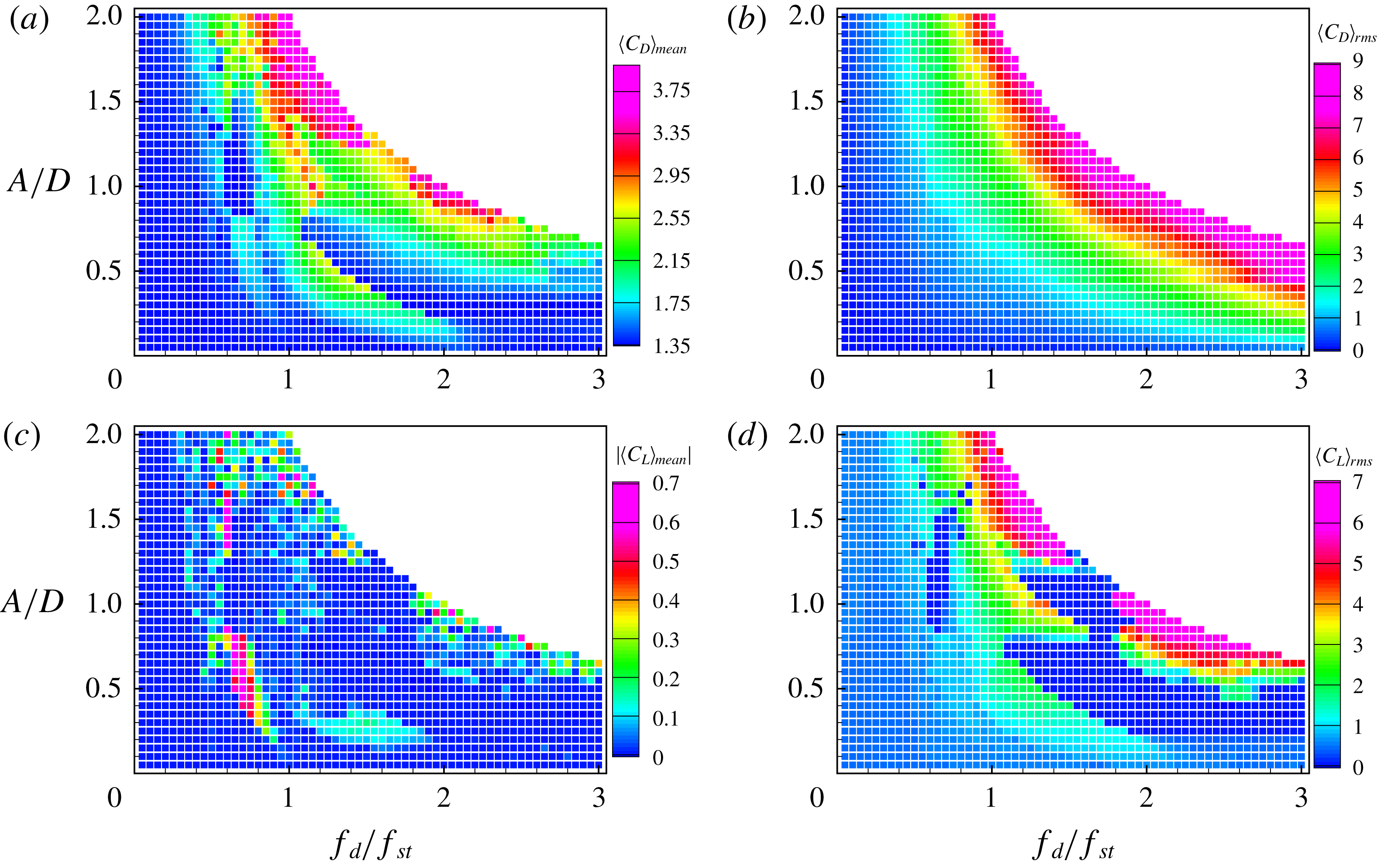
Figure 17(a) shows that
 $\langle C_{D}\rangle _{mean}$
of
 $Re=200$
is larger in non-symmetric harmonic and subharmonic lock-in regions than in non-lock-in regions, similar to
 $\langle C_{D}\rangle _{mean}$
at
 $Re=100$
. In a transitional region from the subharmonic to symmetric harmonic lock-in region,
 $\langle C_{D}\rangle _{mean}$
sharply decreases. In the symmetric harmonic region
 $\langle C_{D}\rangle _{mean}$
gradually increases with increments of either the driving amplitude or frequency. The upper non-lock-in region having a large amplitude and high frequency shows that
 $\langle C_{D}\rangle _{mean}$
becomes more than four times as large as for the non-oscillating cylinder case. Figure 17(b) shows that
 $\langle C_{D}\rangle _{rms}$
at
 $Re=200$
monotonically increases with increase in both the driving amplitude and frequency, similar to
 $\langle C_{D}\rangle _{rms}$
at
 $Re=100$
. Similar to
 $\langle C_{L}\rangle _{mean}$
for
 $Re=100$
, figure 17(c) indicates that
 $\langle C_{L}\rangle _{mean}$
is nearly zero, except in the non-symmetric lock-in region;
 $|\langle C_{L}\rangle _{mean}|$
is less than
 $0.7$
, and its maximum is observed in the non-symmetric lock-in region. Figure 17(d) indicates that
 $\langle C_{L}\rangle _{rms}$
is less than
 $0.8$
in the non-lock-in region, while
 $\langle C_{L}\rangle _{rms}=0.5$
for the non-oscillating case. In the subharmonic lock-in region,
 $\langle C_{L}\rangle _{rms}$
ranges from
 $1$
to
 $4$
. Similar to
 $\langle C_{L}\rangle _{rms}$
at
 $Re=100$
, it is clearly seen that
 $\langle C_{L}\rangle _{rms}\approx 0$
for
 $Re=200$
in the symmetric harmonic lock-in region. For the non-lock-in region with
 $U_{cyl}/U_{0}\geqslant 1.5$
,
 $\langle C_{L}\rangle _{rms}$
increases with the increment of
 $U_{cyl}$
, similar to the behaviour of
 $\langle C_{D}\rangle _{mean}$
in figure 17(a).
Lock-in region map showing the driving amplitude versus the driving frequency at
 $Re=40$
. Lock-in regions and lines are marked in the same manner as in figure 10.
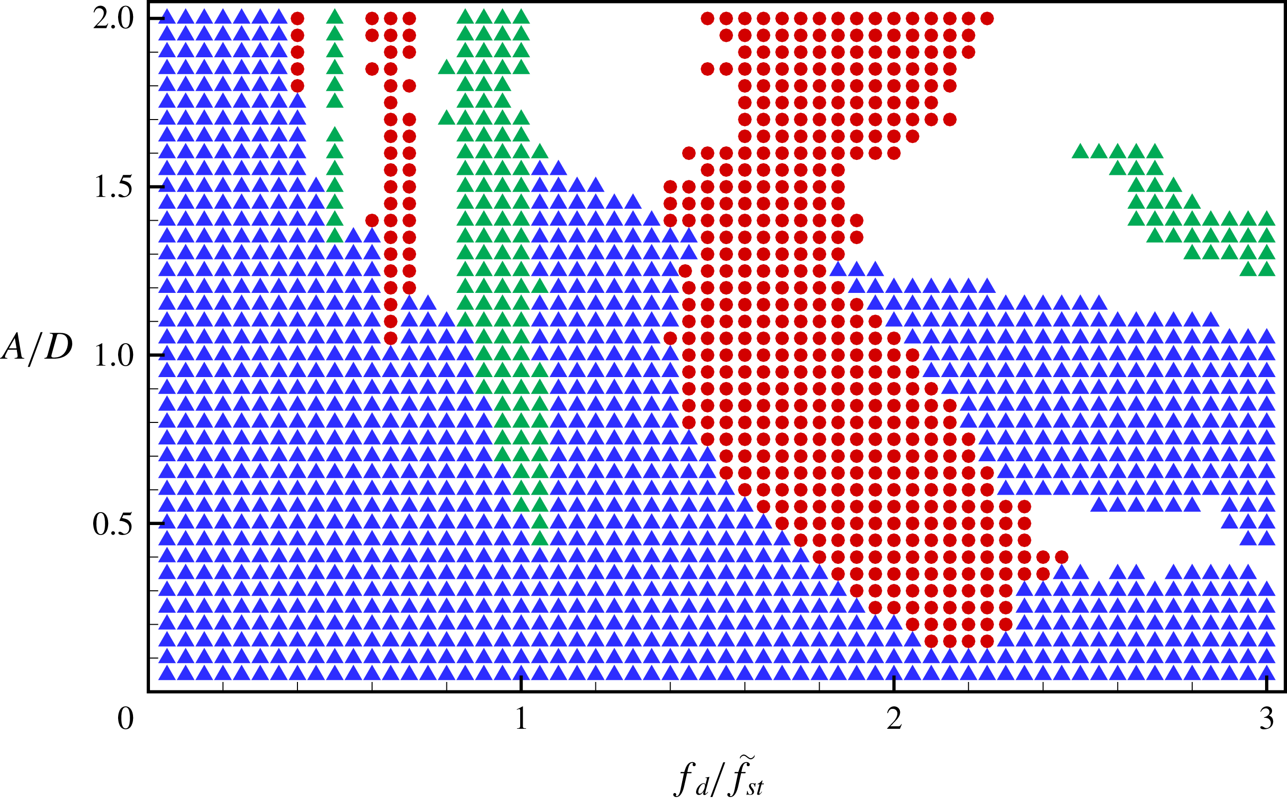
When the Reynolds number is sufficiently low (
 $4\leqslant Re\leqslant 40$
), two small steady separation bubbles appear behind the cylinder. When
 $Re$
increases, the wake behind the cylinder becomes unstable, and experiments have shown that, for
 $Re\geqslant 47$
, the wake develops a slow oscillation in which the velocity is periodic. Since the Strouhal frequency
 $f_{St}$
does not exist at
 $Re=40$
, the driving frequency
 $f_{d}$
for the oscillating cylinder could not be normalized by
 $f_{St}$
. Here, we consider a normalized driving frequency
 $f_{d}/\tilde{f}_{St}$
with the estimated Strouhal frequency
 $\tilde{f}_{St}$
based on the Strouhal–Reynolds number relationship,
 $\tilde{f}_{St}(Re)=Sr^{\ast }+m/\sqrt{Re}$
, where constants
 $Sr^{\ast }$
and
 $m$
are
 $0.2684$
and
 $-1.0356$
, respectively, for
 $47\leqslant Re\leqslant 180$
(Fey, König & Eckelmann Reference Fey, König and Eckelmann1998). The estimated frequency
 $\tilde{f}_{St}$
at
 $Re=40$
is extrapolated from the relationship
 $\tilde{f}_{St}=0.105$
. It should be noted that
 $\tilde{f}_{St}$
has no physical meaning and it is used only for plotting the lock-in region and aerodynamic force maps at
 $Re=40$
in a similar manner to those for
 $Re=100$
and
 $200$
.
Figure 18 indicates that the symmetric harmonic lock-in is found at most driving amplitudes and frequencies at
 $Re=40$
, which is significantly different compared to the lock-in for
 $Re=100$
or
 $200$
. This can be explained by the fact that forced-oscillation-induced inertia is not sufficiently large to introduce asymmetric wake patterns by disturbing the symmetric wake patterns of flow over a stationary cylinder. Although the symmetric harmonic region is dominant at
 $Re=40$
, the subharmonic lock-in region with alternating vortex shedding patterns is found at
 $1.45<f_{d}/f_{St}<2.55$
and
 $A/D\geqslant 0.15$
. The lower boundary of the subharmonic lock-in region for
 $A/D\leqslant 1$
is found at a larger driving amplitude when the driving frequency is shifted to a lower frequency from
 $f_{d}/f_{St}=2$
, whereas the upper boundary is observed at a lower driving frequency for
 $0.3\leqslant A/D\leqslant 1.15$
as
 $A/D$
increases. A non-symmetric harmonic region is observed in a narrow driving frequency range (
 $0.85\leqslant f_{d}/f_{St}\leqslant 1.05$
) for
 $A/D\geqslant 0.45$
, similar to the non-symmetric harmonic regions for
 $Re=100$
and
 $200$
. However, a non-symmetric harmonic region is also found at
 $f_{d}/f_{St}\geqslant 2.5$
and
 $1.15\leqslant A/D\leqslant 1.6$
, which is not observed for
 $Re=100$
and
 $200$
. Three non-lock-in regions are observed in ranges of low amplitudes and high frequencies (
 $0.35\leqslant A/D\leqslant 0.55$
and
 $f_{d}/f_{St}\geqslant 2.4$
), high amplitudes and low frequencies (
 $A/D\geqslant 1.1$
and
 $0.4\leqslant f_{d}/f_{St}\leqslant 0.85$
), and high amplitudes and high frequencies (
 $A/D\geqslant 1.1$
and
 $f_{d}/f_{St}\leqslant 1.1$
).
Time histories of lift coefficient and cylinder position, and snapshots of vorticity for each region during two periods of cylinder motion at
 $Re=40$
. (a) Subharmonic lock-in region
 $(A/D=0.7,~f_{d}/\tilde{f}_{St}=2.0)$
; (b) non-symmetric harmonic lock-in region
 $(A/D=0.7,~f_{d}/\tilde{f}_{St}=1.0)$
; (c) symmetric harmonic lock-in region
 $(A/D=0.7,~f_{d}/\tilde{f}_{St}=2.6)$
; (d) symmetric harmonic lock-in region
 $(A/D=0.7,~f_{d}/\tilde{f}_{St}=1.2)$
; and (e) non-lock-in region
 $(A/D=0.8,~f_{d}/\tilde{f}_{St}=2.6)$
. Vortices are represented in the same manner as in figure 11.
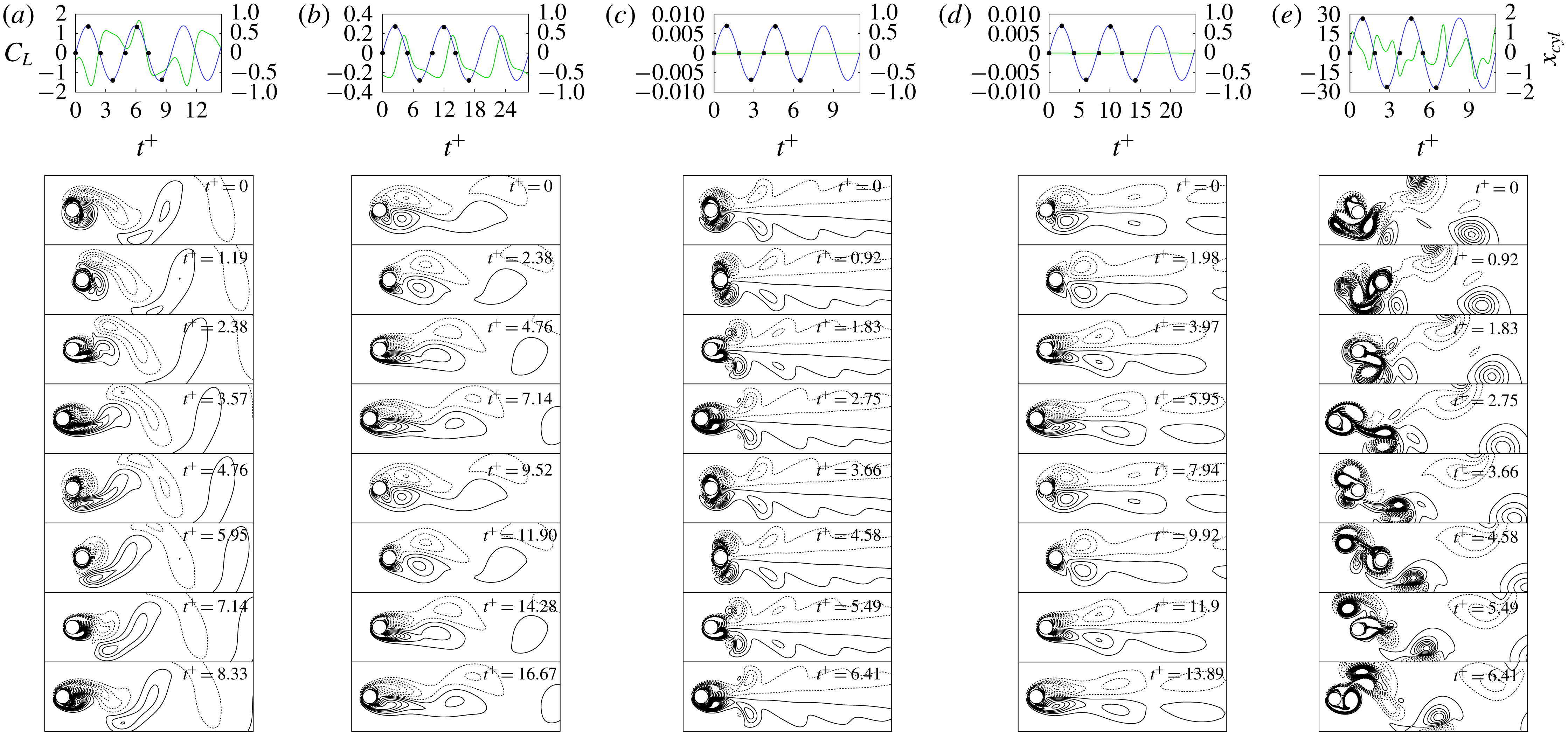
Figure 19 shows wake flow patterns in each distinct region at
 $Re=40$
. Figures 19(a), 19(b), 19(c) and 19(e) show subharmonic lock-in, non-symmetric harmonic lock-in, symmetric harmonic lock-in and non-lock-in regions, respectively, like those observed in figures 11 and 16 for
 $Re=100$
and
 $200$
. However, it should be noted that figure 19(d) shows a flow pattern in the symmetric harmonic lock-in region at
 $Re=40$
, in contrast to those of the non-lock-in mode shown in figures 11(d) and 16(d) for
 $Re=100$
and
 $200$
. This is because the flow behind the non-oscillatory cylinder at
 $Re=40$
induces a stationary pattern with small steady separation bubbles. Thus, the symmetric harmonic region is observed at most driving amplitudes and frequencies, even where non-lock-in regions are observed at
 $Re=100$
and
 $200$
. The flow patterns in the subharmonic region at
 $Re=40$
, shown in figure 19(a), show that the two counter-rotating vortices are alternately detached at the upper and lower parts of the cylinder. One cycle of the vortex pattern is completed by two cycles of the cylinder oscillation, similar to that observed in the subharmonic regions of
 $Re=100$
and
 $200$
. Furthermore, the peaks of the lift coefficient are observed at the instants at which the cylinder changes its oscillating direction. Figure 19(b) shows flow patterns in the non-symmetric harmonic region at
 $Re=40$
. Similar to the flow patterns in the non-symmetric harmonic region at
 $Re=100$
and
 $200$
, a pair of vortices are formed as the cylinder moves downstream, whereas the vortices are detached as the cylinder moves upstream. The pair of two counter-rotating vortices is not symmetric, which leads to a non-zero mean lift coefficient. A periodic vortex shedding is clearly observed, and the shedding pattern is completed within one cycle of the cylinder oscillation. The flow patterns for symmetric harmonic lock-in are clearly shown in figure 18(c,d), thus not yielding any lift force. The case of the low-frequency oscillation
 $\tilde{f}_{St}=1.0$
in figure 19(c) indicates that two dominant CW and ACW rotating vortices are formed near the cylinder moving upstream, and they are quickly separated from the cylinder moving downstream; this is similar to the behaviour of wake flows in the symmetric harmonic lock-in region for
 $Re=100$
and
 $200$
. However, figure 19(d) for wake flows of the oscillatory cylinder with a high frequency
 $\tilde{f}_{St}=2.6$
shows that two dominant counter-rotating vortices are elongated further downstream while maintaining symmetry. This is a different observation, compared to the wake patterns in the symmetric harmonic lock-in region for other cases. Moreover, it is worth noting that non-lock-in was observed for
 $Re=100$
and
 $200$
at a similar oscillation condition. Flow patterns induced by a highly oscillating cylinder at
 $Re=40$
are shown in figure 19(e). Similar to the flow patterns at
 $Re=100$
and
 $200$
with a high oscillation amplitude and frequency, complex wake patterns are found due to the disordered vortex shedding. This leads to large variations in the lift coefficient.
Aerodynamic force maps of an oscillating cylinder in
 $A/D{-}f_{d}/f_{St}$
space for (a)
 $\langle C_{D}\rangle _{mean}$
, (b)
 $\langle C_{D}\rangle _{rms}$
, (c)
 $|\langle C_{L}\rangle _{mean}|$
, and (d)
 $\langle C_{L}\rangle _{rms}$
values at
 $Re=40$
.
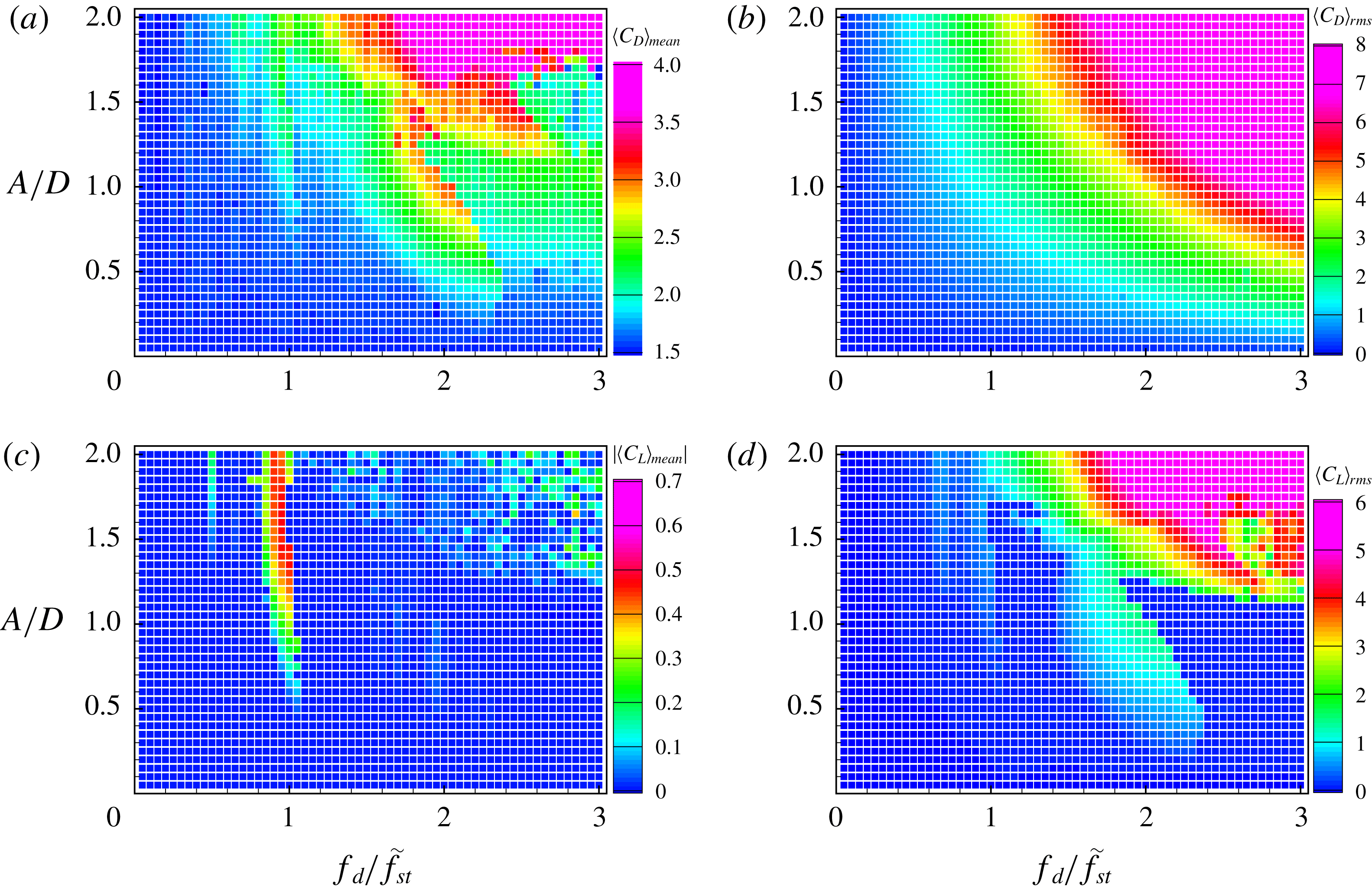
Figure 20(a) shows that the overall trends of
 $\langle C_{D}\rangle _{mean}$
for
 $Re=40$
are similar to those for
 $Re=100$
and
 $200$
. Owing to the streamwise oscillatory cylinder motion,
 $\langle C_{D}\rangle _{mean}$
is increased compared to that in the non-oscillating case. At the upper boundary of the subharmonic region,
 $\langle C_{D}\rangle _{mean}$
sharply decreases as the cylinder acceleration increases, which is similar to that at
 $Re=100$
. It is noticeable that
 $\langle C_{D}\rangle _{mean}$
in the non-lock-in region with a large amplitude and high frequency (
 $A/D\geqslant 1.5$
and
 $f_{d}/f_{St}\leqslant 1.1$
) is more than 2.5 times greater than that in other regions, which is mainly because of the forced inertial effects. Interestingly,
 $\langle C_{D}\rangle _{mean}$
is relatively small and approximately 1.9 in the non-symmetric harmonic region with
 $f_{d}/f_{St}\geqslant 2.5$
for
 $1.15\leqslant A/D\leqslant 1.6$
. This is because the cylinder-oscillation-induced counter-rotating vortices are detached fairly far from the cylinder and have relatively low influence on the drag. Figure 20(b) shows that
 $\langle C_{D}\rangle _{rms}$
at
 $Re=40$
monotonically increases with increase in both the driving amplitude and frequency, similar to
 $\langle C_{D}\rangle _{rms}$
at
 $Re=100$
and
 $200$
. Figure 20(c) indicates that a non-zero
 $\langle C_{L}\rangle _{mean}$
is only found in the non-symmetric lock-in region, similar to the cases of
 $Re=100$
and
 $200$
. Except for oscillating cases with a high cylinder acceleration (roughly
 $1.25\leqslant A/D$
and
 $f_{d}/f_{St}\geqslant 1.5$
), figure 20(d) shows that
 $\langle C_{L}\rangle _{rms}$
is nearly zero in most cases because the symmetric harmonic lock-in is dominant at
 $Re=40$
. However, in the subharmonic region,
 $\langle C_{L}\rangle _{rms}$
gradually increases with increase in both the amplitude and frequency, which is similar to the cases of
 $Re=100$
and
 $200$
. In the non-lock-in region for the case of a highly accelerating cylinder (
 $A/D\geqslant 1.5$
and
 $f_{d}/f_{St}\leqslant 1.1$
),
 $\langle C_{L}\rangle _{rms}$
is significantly larger (more than 4) because higher inertial effects due to the cylinder motion promote asymmetric and alternating vortex shedding behind the cylinder. However,
 $\langle C_{L}\rangle _{rms}$
is relatively small in the non-symmetric lock-in region for the case of a highly accelerating cylinder.
The effect of
 $Re$
on the lock-in phenomenon for flow over a streamwise oscillatory cylinder is summarized as follows: subharmonic lock-in, symmetric harmonic lock-in, non-symmetric harmonic lock-in and non-lock-in regions are found at all three
 $Re$
numbers. For both
 $Re=100$
and
 $200$
, the threshold amplitude of the subharmonic lock-in region agrees with that given by Leontini et al. (Reference Leontini, Jacono and Thompson2013). For a small driving amplitude (
 $A/D\leqslant 0.75$
), the symmetric harmonic region is found at
 $1.0\leqslant U_{cyl}/U_{0}\leqslant 1.5$
for both
 $Re=100$
and
 $200$
. In particular, for
 $Re=200$
the subharmonic region is also found in
 $0.75<A/D<1.2$
and
 $1.0\leqslant U_{cyl}/U_{0}\leqslant 1.5$
, and the non-lock-in regions exist at a high driving amplitude
 $A/D>1.75$
regardless of driving frequency. For
 $Re=40$
, the symmetric harmonic lock-in is found at most driving amplitudes and frequencies. The non-symmetric harmonic lock-in region is found at
 $f_{d}/f_{St}\geqslant 2.5$
and
 $1.15\leqslant A/D\leqslant 1.6$
for
 $Re=40$
, whereas the non-symmetric harmonic lock-in region is mostly found near the Strouhal frequency (approximately
 $0.8<f_{d}/f_{St}<1$
) for all three
 $Re$
numbers. Similar flow patterns are found at all three
 $Re$
numbers, depending on the lock-in regions. In the subharmonic lock-in region, two alternating vortex shedding patterns are synchronized with two cycles of the cylinder motion. In the non-symmetric harmonic lock-in region, two counter-rotating vortices induced by the cylinder moving upstream are convected downstream in a slightly upward- or downward-shifted direction, which leads to a non-zero mean lift force. For symmetric lock-in, two pairs of counter-rotating vortices are symmetrically formed near the cylinder and convected downstream while their strengths are weakened. In particular, a different type of symmetric lock-in is observed only for
 $Re=40$
with a high driving frequency, where two dominant counter-rotating vortices are elongated further downstream while forming a larger separation bubble. In the non-lock-in region, the vortex shedding cycle is incomplete during the two periods of the cylinder oscillation. Depending on
 $Re$
, the symmetric patterns in the wake flows are slightly different for the moderate driving amplitude and frequency. However, wake flows with a large driving amplitude and high driving frequency show disordered vortex shedding patterns, which induce large lift fluctuations. The overall trends of the aerodynamic forces with a driving amplitude and frequency can be characterized as per the distinctive lock-in region. The values of
 $\langle C_{D}\rangle _{mean}$
are larger in the subharmonic region than those in other regions, and larger driving amplitude and higher driving frequency lead to an increased
 $\langle C_{D}\rangle _{rms}$
. Except for the non-symmetric harmonic lock-in case,
 $\langle C_{L}\rangle _{mean}$
is almost zero; and
 $\langle C_{L}\rangle _{rms}$
has a large value in the subharmonic region whereas it is relatively small in the non-symmetric harmonic lock-in region.
5 Conclusion
Numerical simulations were performed for flow over a circular cylinder oscillating streamwise at various driving amplitudes and frequencies in order to identify lock-in regions. We considered three different Reynolds numbers (
 $Re=40,100$
and
 $200$
) with the driving amplitude and frequency in the ranges
 $A/D=0.05{-}2.0$
and
 $f_{d}/f_{St}=0.05{-}3.0$
, respectively. The Fourier spectrum of the lift coefficient was used to define lock-in as regions where the spectrum peaks are sharply converged to
 $f_{d}$
. The present study showed that there are two types of lock-in: one is lock-in where spectrum peaks are converged to
 $f/f_{d}=1/2+n$
, which is called subharmonic lock-in; and the other is harmonic lock-in where spectrum peaks are converged to
 $f/f_{d}=1+n$
, with
 $n=0,1,2,\ldots ,\infty$
. The oscillating conditions for which lock-in phenomena occur were marked on a non-dimensional driving amplitude–frequency plane. These maps classify the lock-in regions: one is a subharmonic lock-in region, and the others are a non-symmetric harmonic region and a symmetric harmonic region. The features of aerodynamic forces at each region are characterized by the distributions of mean and r.m.s. values of drag and lift coefficients with respect to the driving amplitude and frequency.
The subharmonic lock-in region was found in a lower frequency range when the driving amplitude was increased. The lower threshold amplitude of the subharmonic lock-in region follows the characteristic line proposed by Leontini et al. (Reference Leontini, Jacono and Thompson2013). Alternating vortex shedding patterns are dominant in the subharmonic region for
 $Re=100$
and
 $200$
. Interestingly, the subharmonic lock-in was also observed at
 $Re=40$
for
 $1.45<f_{d}/f_{St}<2.55$
. In the subharmonic lock-in region,
 $\langle C_{D}\rangle _{mean}$
and
 $\langle C_{L}\rangle _{rms}$
are evidently increased by forced cylinder oscillations. The non-symmetric harmonic region was observed near the Strouhal frequency (approximately
 $0.8<f_{d}/f_{St}<1$
), where counter-rotating vortices do not symmetrically form behind the cylinder, yielding non-zero values of
 $\langle C_{L}\rangle _{mean}$
. The symmetric harmonic region for
 $Re=100$
is bounded in
 $1.0\leqslant U_{cyl}/U_{0}\leqslant 1.5$
, while two symmetric harmonic regions (
 $A/D\leqslant 0.75$
in
 $1.0\leqslant U_{cyl}/U_{0}\leqslant 1.5$
and
 $0.75\leqslant A/D\leqslant 1.25$
in
 $1.5\leqslant U_{cyl}/U_{0}\leqslant 2.0$
) were observed for
 $Re=200$
. However, most oscillating cases for
 $Re=40$
showed symmetric harmonic lock-in because the vortex patterns induced by oscillating cylinder motion are not sufficient to destroy the symmetric behaviour of wake patterns originating from the non-oscillating case. Owing to the vertically symmetric vortex pattern,
 $\langle C_{L}\rangle _{rms}$
values are almost zero in the symmetric harmonic lock-in region. Overall,
 $\langle C_{D}\rangle _{rms}$
monotonically increases with both the driving amplitude and frequency, irrespective of the lock-in patterns.
In summary, we found that the subharmonic lock-in region due to a small driving amplitude and low frequency at
 $Re=100$
and
 $200$
is similar to that identified in Leontini et al. (Reference Leontini, Jacono and Thompson2013), where the threshold amplitude (Leontini et al.
Reference Leontini, Jacono and Thompson2013) of the subharmonic lock-in depends on
 $Re$
. The subharmonic lock-in region is also found even at
 $Re=40$
where steady wake flows are observed for a stationary cylinder. Moreover, the present parametric study with a wide range of driving forces shows that a new lock-in region (non-symmetric harmonic lock-in region) exists for a large driving amplitude, whereas a different lock-in region (symmetric harmonic lock-in region) is observed at a high driving frequency.
Acknowledgements
The authors are grateful to the anonymous referees whose valuable suggestions and comments significantly improved the quality of this paper. This work was supported by the National Research Foundation of Korea (NRF) grant funded by the Korean government (Ministry of Science and ICT) (NRF-20151009350) and in part by Yonsei University.
Appendix A. Note on resolution requirements
Effect of the radial grid resolution on drag and lift coefficients for the case of
 $A/D=1.0$
and
 $f_{d}/f_{St}=2.4$
 $(U_{cyl}/U_{0}=2.48)$
at
 $Re=100$
.
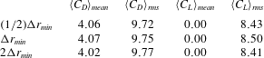
We have performed a grid resolution study for the case of a highly oscillating cylinder in which the maximum speed of the oscillating cylinder is
 $U_{max}/U_{0}=2.48$
; the case of
 $A/D=1.0$
and
 $f_{d}/f_{St}=2.4$
. As a baseline grid, a non-uniform grid with
 $256$
points is used in the radial direction, whereas a uniform grid with
 $\unicode[STIX]{x0394}\unicode[STIX]{x1D703}=2\unicode[STIX]{x03C0}/256$
is used in the circumferential direction. The minimum and maximum grid spacings in the radial direction are set to
 $\unicode[STIX]{x0394}r_{min}=0.0016$
and
 $\unicode[STIX]{x0394}r_{max}=0.2$
, respectively. For the grid resolution study, we consider three different grid spacings in the radial direction by setting the minimum grid spacing to
 $\unicode[STIX]{x0394}r_{min}$
,
 $(1/2)\unicode[STIX]{x0394}r_{min}$
and
 $2\unicode[STIX]{x0394}r_{min}$
. Table 2 indicates no significant difference pertaining to the mean and r.m.s. values of
 $C_{D}$
and
 $C_{L}$
obtained from numerical simulations with different grid resolutions.
Effect of grid resolutions on
 $C_{L}$
for different lock-in regions: (a–c) subharmonic lock-in region
 $(A/D=0.4,~f_{d}/f_{St}=1.5)$
, (d–f) non-symmetric harmonic lock-in region
 $(A/D=0.4,~f_{d}/f_{St}=0.8)$
, (g–i) symmetric harmonic lock-in region
 $(A/D=0.4,~f_{d}/f_{St}=2.8)$
, (j–l) non-lock-in region
 $(A/D=0.4,~f_{d}/f_{St}=1.9)$
, and (m–o) non-lock-in region
 $(A/D=0.9,~f_{d}/f_{St}=2.4)$
.
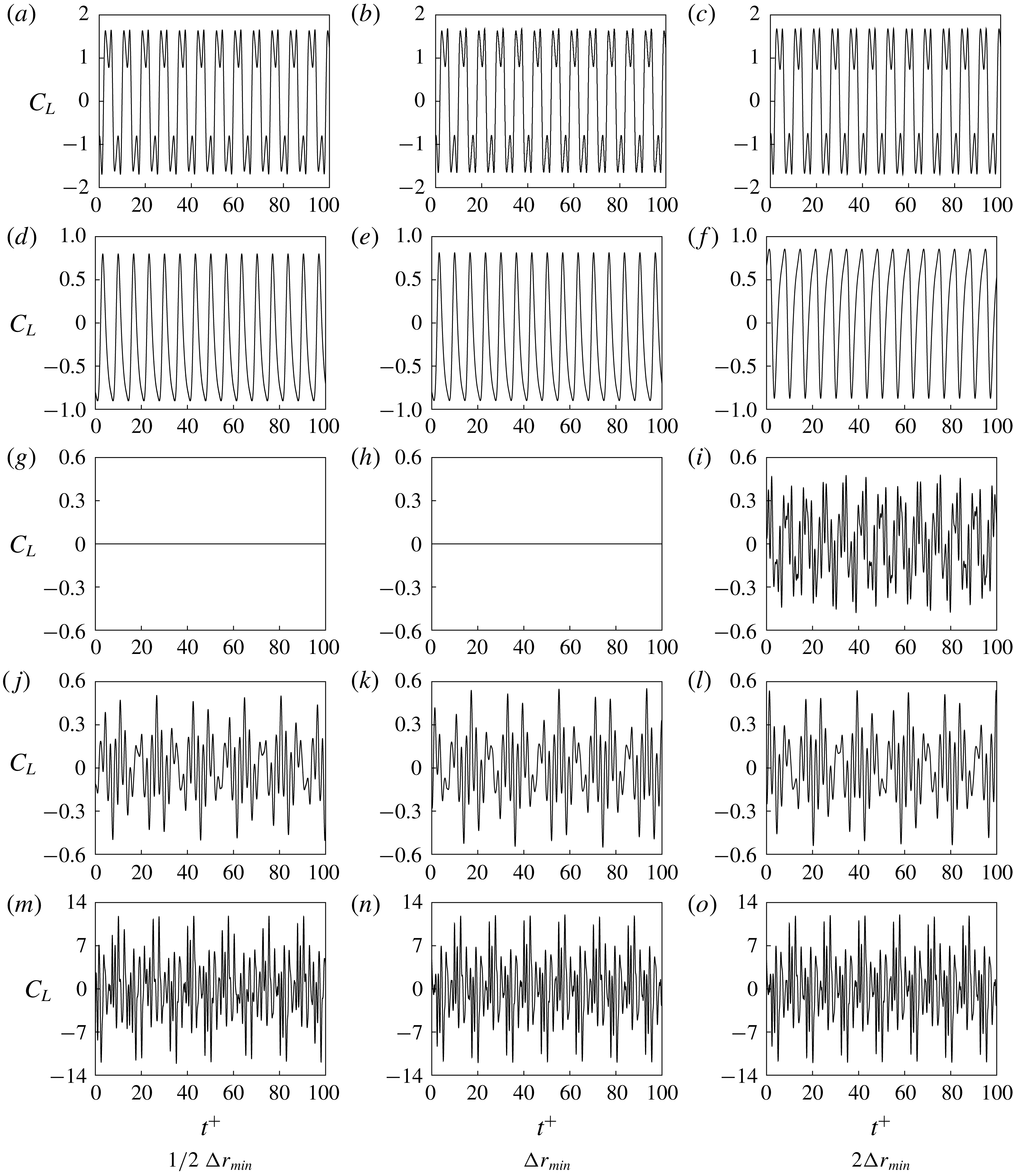
We also investigated the effect of grid resolutions on the classification of lock-in regions. To this end, we performed numerical simulations of five different lock-in cases that are shown in figure 11 for
 $Re=100$
. The rows and columns in figure 21 indicate the time histories of
 $C_{L}$
for different lock-in regions and grid resolutions, respectively. Except for the case of the symmetric harmonic lock-in region, numerical simulations with all three grid resolutions provide a similar trend of temporal variations of
 $C_{L}$
. This confirms that time histories of
 $C_{L}$
obtained from numerical simulations with the present grid resolution
 $(\unicode[STIX]{x0394}r_{min})$
are identical to those obtained with a finer grid resolution
 $((1/2)\unicode[STIX]{x0394}r_{min})$
, leading to the same classification of the lock-in phenomenon.
Appendix B. Formulae for drag and lift coefficients
This appendix provides the formulae of drag and lift coefficients for flow over a circular cylinder. The drag (
 $C_{D}$
) and lift (
 $C_{L}$
) coefficients can be defined as
 $$\begin{eqnarray}C_{D}=\frac{F_{x}}{\frac{1}{2}\unicode[STIX]{x1D70C}{U_{0}}^{2}D}\quad \text{and}\quad C_{L}=\frac{F_{y}}{\frac{1}{2}\unicode[STIX]{x1D70C}{U_{0}}^{2}D},\end{eqnarray}$$
where
 $F_{x}$
and
 $F_{y}$
are the streamwise and transverse components of the force
 $\boldsymbol{F}$
induced by the flow, respectively,
 $U_{0}$
is the free-stream velocity,
 $\unicode[STIX]{x1D70C}$
is the density of fluid and
 $D$
is the diameter of the cylinder. Force
 $\boldsymbol{F}$
can be obtained by integrating the pressure and the normal and shear stresses acting on the cylinder surface in cylindrical coordinates
 $(r_{0},\unicode[STIX]{x1D703})$
:
 $$\begin{eqnarray}\displaystyle & \displaystyle F_{x}=\int _{0}^{2\unicode[STIX]{x03C0}}(-\hat{p}(r_{0},\unicode[STIX]{x1D703})\cos \unicode[STIX]{x1D703}+\hat{\unicode[STIX]{x1D70E}}_{rr}(r_{0},\unicode[STIX]{x1D703})\cos \unicode[STIX]{x1D703}-\hat{\unicode[STIX]{x1D70E}}_{r\unicode[STIX]{x1D703}}(r_{0},\unicode[STIX]{x1D703})\sin \unicode[STIX]{x1D703})r_{0}\,\text{d}\unicode[STIX]{x1D703}, & \displaystyle\end{eqnarray}$$
 $$\begin{eqnarray}\displaystyle & \displaystyle F_{y}=\int _{0}^{2\unicode[STIX]{x03C0}}(-\hat{p}(r_{0},\unicode[STIX]{x1D703})\sin \unicode[STIX]{x1D703}+\hat{\unicode[STIX]{x1D70E}}_{rr}(r_{0},\unicode[STIX]{x1D703})\sin \unicode[STIX]{x1D703}+\hat{\unicode[STIX]{x1D70E}}_{r\unicode[STIX]{x1D703}}(r_{0},\unicode[STIX]{x1D703})\cos \unicode[STIX]{x1D703})r_{0}\,\text{d}\unicode[STIX]{x1D703}, & \displaystyle\end{eqnarray}$$
where
 $r_{0}$
indicates the cylinder surface
 $(r_{0}=D/2)$
. Note that
 $\hat{p}$
,
 $\hat{\unicode[STIX]{x1D70E}}_{rr}$
and
 $\hat{\unicode[STIX]{x1D70E}}_{r\unicode[STIX]{x1D703}}$
represent the dimensional pressure, and normal and shear stress, respectively:
 $$\begin{eqnarray}\hat{p}=\unicode[STIX]{x1D70C}{U_{0}}^{2}p,\quad \hat{\unicode[STIX]{x1D70E}}_{rr}=2\frac{\unicode[STIX]{x1D707}U_{0}}{D}\frac{\unicode[STIX]{x2202}U_{r}}{\unicode[STIX]{x2202}r}\quad \text{and}\quad \hat{\unicode[STIX]{x1D70E}}_{r\unicode[STIX]{x1D703}}=\frac{\unicode[STIX]{x1D707}U_{0}}{D}\frac{\unicode[STIX]{x2202}U_{\unicode[STIX]{x1D703}}}{\unicode[STIX]{x2202}r},\end{eqnarray}$$
where
 $\unicode[STIX]{x1D707}$
is dynamic viscosity, and
 $U_{r}$
and
 $U_{\unicode[STIX]{x1D703}}$
represent the dimensionless radial and azimuthal velocity components, respectively, in the inertial system. Finally,
 $C_{D}$
and
 $C_{L}$
can be defined as
 $$\begin{eqnarray}\displaystyle & \displaystyle C_{D}=\int _{0}^{2\unicode[STIX]{x03C0}}\left(-p(r_{0},\unicode[STIX]{x1D703})\cos \unicode[STIX]{x1D703}+\frac{2}{Re}\left.\frac{\unicode[STIX]{x2202}U_{r}}{\unicode[STIX]{x2202}r}\right|_{(r_{0},\unicode[STIX]{x1D703})}\cos \unicode[STIX]{x1D703}-\frac{1}{Re}\left.\frac{\unicode[STIX]{x2202}U_{\unicode[STIX]{x1D703}}}{\unicode[STIX]{x2202}r}\right|_{(r_{0},\unicode[STIX]{x1D703})}\sin \unicode[STIX]{x1D703}\right)r_{0}\,\text{d}\unicode[STIX]{x1D703},\quad & \displaystyle\end{eqnarray}$$
 $$\begin{eqnarray}\displaystyle & \displaystyle C_{L}=\int _{0}^{2\unicode[STIX]{x03C0}}\left(-p(r_{0},\unicode[STIX]{x1D703})\sin \unicode[STIX]{x1D703}+\frac{2}{Re}\left.\frac{\unicode[STIX]{x2202}U_{r}}{\unicode[STIX]{x2202}r}\right|_{(r_{0},\unicode[STIX]{x1D703})}\sin \unicode[STIX]{x1D703}+\frac{1}{Re}\left.\frac{\unicode[STIX]{x2202}U_{\unicode[STIX]{x1D703}}}{\unicode[STIX]{x2202}r}\right|_{(r_{0},\unicode[STIX]{x1D703})}\cos \unicode[STIX]{x1D703}\right)r_{0}\,\text{d}\unicode[STIX]{x1D703}.\quad & \displaystyle\end{eqnarray}$$



