





Introduction
Potato (Solanum tuberosum L.) is the fourth most consumed crop in the world and in Europe, it serves as a staple food, plays a key role in animal feeding, and therefore is a critical part of the diet and agricultural economy (FAO, 2021). Due to the high sensitivity of potatoes to climatic variability (Haverkort and Verhagen, Reference Haverkort and Verhagen2008), potato yield is greatly affected by weather and climate situations (Hijmans, Reference Hijmans2003; Raymundo et al., Reference Raymundo, Asseng, Robertson, Petsakos, Hoogenboom, Quiroz, Hareau and Wolf2018; Zabel et al., Reference Zabel, Müller, Elliott, Minoli, Jägermeyr, Schneider, Franke, Moyer, Dury, Francois, Folberth, Liu, Pugh, Olin, Rabin, Mauser, Hank, Ruane and Asseng2021). According to the IPCC Sixth Assessment Report (2021), large-scale climate modes such as the El Niño–Southern Oscillation (ENSO), Arctic Oscillation (AO), North Atlantic Oscillation (NAO), and Scandinavian Pattern (SCA) exert strong influence on regional climate variability and extreme weather events across Europe and beyond. Under continued global warming, the frequency and intensity of extreme phases of these teleconnections, particularly ENSO, are projected to increase, amplifying their impact on agricultural systems and adaptation challenges (IPCC, 2021). During the last decade, several studies have explored teleconnection effects to better understand their influence on regional climate conditions (Gonsamo and Chen, Reference Gonsamo and Chen2015; Hurrell et al., Reference Hurrell, Kushnir, Ottersen and Visbeck2003; Trenberth et al., Reference Trenberth, Fasullo and Shepherd2014a). These teleconnection patterns control the critical factors for crop growth including temperature, precipitation, and seasonal variability (Monaghan et al., Reference Monaghan, Daccache, Vickers, Hess, Weatherhead, Grove and Knox2013; Raymundo et al., Reference Raymundo, Asseng, Robertson, Petsakos, Hoogenboom, Quiroz, Hareau and Wolf2018), which can lead to changes in planting seasons and variations in agricultural yield productivity (Olesen et al., Reference Olesen, Trnka, Kersebaum, Skjelvåg, Seguin, Peltonen-Sainio, Rossi, Kozyra and Micale2011; Zabel et al., Reference Zabel, Müller, Elliott, Minoli, Jägermeyr, Schneider, Franke, Moyer, Dury, Francois, Folberth, Liu, Pugh, Olin, Rabin, Mauser, Hank, Ruane and Asseng2021). In this context, understanding how teleconnections shape the production of major food crops such as potato is increasingly important for safeguarding European food security and designing robust climate adaptation strategies.
Due to Europe’s diverse climates, ranging from the cold northern regions with shorter growing seasons to the more moderate conditions in central and southern areas (Trnka et al., Reference Trnka, Olesen, Kersebaum, Skjelvåg, Eitzinger, Seguin, Peltonen-Sainio, Rötter, Iglesias, Orlandini, Dubrovský, Hlavinka, Balek, Eckersten, Cloppet, Calanca, Gobin, Vučetić, Nejedlik, Kumar, Lalic, Mestre, Rossi, Kozyra, Alexandrov, Semerádová and Žalud2011; Zabel et al., Reference Zabel, Müller, Elliott, Minoli, Jägermeyr, Schneider, Franke, Moyer, Dury, Francois, Folberth, Liu, Pugh, Olin, Rabin, Mauser, Hank, Ruane and Asseng2021), a region-specific approach may provide a more reliable method to identify how teleconnections affect potato productivity. Additionally, it’s notable that teleconnection patterns do not always produce direct impacts, as soil moisture, temperature, and rainfall can be influenced by the atmosphere and ocean variations in earlier months (García-Herrera et al., Reference García-Herrera, Paredes, Trigo, Trigo, Hernández, Barriopedro and Mendes2007). Therefore, it is important to consider the lagged effect of teleconnections for agricultural forecasting (Monaghan et al., Reference Monaghan, Daccache, Vickers, Hess, Weatherhead, Grove and Knox2013; Raymundo et al., Reference Raymundo, Asseng, Robertson, Petsakos, Hoogenboom, Quiroz, Hareau and Wolf2018). Teleconnection-sensitive regional risk profiles and climate “memory” effects are particularly relevant for early warning and strategic planning at multi-season to multi-year horizons.
Traditional statistical models often struggle to explain the nonlinear and complex effects of large-scale climatic teleconnections on agricultural productivity (Hu et al., Reference Hu, Zhang, Khanal, Wilson, Leng, Toman and Zhao2024). However, using advanced machine learning (ML) algorithms leads to a data-driven approach capable of extracting patterns and enhancing prediction accuracy (Chen and Guestrin, Reference Chen and Guestrin2016; Ke et al., Reference Ke, Meng, Finley, Wang, Chen, Ma, Ye and Liu2017). Several studies have also confirmed the good result of different ML algorithms, such as Random Forest and XGBoost, used for crop yield prediction (Elbasi et al., Reference Elbasi, Zaki, Topcu, Abdelbaki, Zreikat, Cina, Shdefat and Saker2023; Leukel et al., Reference Leukel, Zimpel and Stumpe2023; Naghdyzadegan Jahromi et al., Reference Naghdyzadegan Jahromi, Zand-Parsa, Razzaghi, Jamshidi, Didari, Doosthosseini and Pourghasemi2023; Rao et al., Reference Rao, Singh, Reddy and Acharya2022; Van Klompenburg et al., Reference Van Klompenburg, Kassahun and Catal2020). Some studies have examined the impact of climate change and teleconnections on different crops across Europe; for instance, Ceglar et al. (Reference Ceglar, Turco, Toreti and Doblas-Reyes2017) indicated that teleconnections cause 38% and 43% of the variability in maize and winter wheat across Europe. Also, different researchers explored the effects of climate change on different crops like wheat (Asseng et al., Reference Asseng, Ewert, Rosenzweig, Jones, Hatfield, Ruane, Boote, Thorburn, Rötter, Cammarano, Brisson, Basso, Martre, Aggarwal, Angulo, Bertuzzi, Biernath, Challinor, Doltra, Gayler, Goldberg, Grant, Heng, Hooker, Hunt, Ingwersen, Izaurralde, Kersebaum, Müller, Naresh Kumar, Nendel, O’Leary, Olesen, Osborne, Palosuo, Priesack, Ripoche, Semenov, Shcherbak, Steduto, Stöckle, Stratonovitch, Streck, Supit, Tao, Travasso, Waha, Wallach, White, Williams and Wolf2013; Trnka et al., Reference Trnka, Olesen, Kersebaum, Skjelvåg, Eitzinger, Seguin, Peltonen-Sainio, Rötter, Iglesias, Orlandini, Dubrovský, Hlavinka, Balek, Eckersten, Cloppet, Calanca, Gobin, Vučetić, Nejedlik, Kumar, Lalic, Mestre, Rossi, Kozyra, Alexandrov, Semerádová and Žalud2011; Trnka et al., Reference Trnka, Rötter, Ruiz-Ramos, Kersebaum, Olesen, Žalud and Semenov2014), barley (Moore and Lobell, Reference Moore and Lobell2015; Schmidt and Felsche, Reference Schmidt and Felsche2024), sugar beet (Guimarães Nobre et al., Reference Guimarães Nobre, Hunink, Baruth, Aerts and Ward2019), and Maize (Schmidt and Felsche, Reference Schmidt and Felsche2024). Yet, few studies have combined multi-decadal teleconnection records, long lag structures, and explainable ML techniques specifically for potato, and even fewer have done so at the European scale.
Despite the recognized influence of large-scale climate modes on European climate (Hurrell et al., Reference Hurrell, Kushnir, Ottersen and Visbeck2003; Trenberth et al., Reference Trenberth, Fasullo and Shepherd2014a), their role in driving potato yield variability remains underexplored, particularly at the continental scale and over long time periods. Existing studies have mainly focused on other crops (e.g., wheat, maize, sugar beet) or on shorter time windows and often rely on traditional statistical models that only partly capture nonlinear and lagged teleconnection effects.
Traditional crop yield models often rely on local meteorological variables such as temperature, precipitation, and soil moisture. While these variables directly influence crop growth, they represent local expressions of broader atmospheric and oceanic circulation. In contrast, teleconnection indices describe upstream climate variability and may provide earlier warning signals at seasonal-to-multi-year time scales (Ceglar et al., Reference Ceglar, Turco, Toreti and Doblas-Reyes2017). Therefore, this study intentionally evaluates the predictive information contained in teleconnection indices alone, rather than combining them with local meteorological variables. This approach does not replace process-based or meteorological crop yield modeling but complements it by assessing whether large-scale climate modes can support regional yield-risk prediction. This research aims to fill this gap by using state-of-the-art ML and explainable AI to explore the relationship between teleconnection indices and potato yield across Europe from 1961 to 2023. Specifically, the study seeks to: (i) quantify the influence of multiple teleconnection indices, including their lagged effects, on potato yield in three major European regions (North, Central, and South); (ii) develop and evaluate a suite of ML models to improve regional yield predictions; and (iii) identify the most influential teleconnection patterns using SHapley Additive exPlanations (SHAP) and assess how their impacts vary among regions. By linking teleconnection-driven yield variability to a major staple crop, the study provides a scientific basis for teleconnection-aware forecasting, climate-risk management, and food security planning in Europe.
Materials and methods
Study area
With its differing climatic conditions and agricultural practices, Europe provides a unique research environment for studying the impact of teleconnection patterns on potato yield. Potato is produced in all sorts of climatic conditions, influencing planting calendars, growing seasons, and yield productivity (Olesen et al., Reference Olesen, Trnka, Kersebaum, Skjelvåg, Seguin, Peltonen-Sainio, Rossi, Kozyra and Micale2011; Raymundo et al., Reference Raymundo, Asseng, Robertson, Petsakos, Hoogenboom, Quiroz, Hareau and Wolf2018; Zabel et al., Reference Zabel, Müller, Elliott, Minoli, Jägermeyr, Schneider, Franke, Moyer, Dury, Francois, Folberth, Liu, Pugh, Olin, Rabin, Mauser, Hank, Ruane and Asseng2021). Accordingly, this paper divides Europe into three subzones (Northern Europe, Central Europe, Southern Europe; Figure 1) to reflect these regional features. Subzoning was based on the potato growing season period, as well as on specific climatic conditions that characterize each region (Goffart et al., Reference Goffart, Haverkort, Storey, Haase, Martin, Lebrun, Ryckmans, Florins and Demeulemeester2022; Hijmans, Reference Hijmans2003; Obidiegwu et al., Reference Obidiegwu, Bryan, Jones and Prashar2015; Trnka et al., Reference Trnka, Olesen, Kersebaum, Skjelvåg, Eitzinger, Seguin, Peltonen-Sainio, Rötter, Iglesias, Orlandini, Dubrovský, Hlavinka, Balek, Eckersten, Cloppet, Calanca, Gobin, Vučetić, Nejedlik, Kumar, Lalic, Mestre, Rossi, Kozyra, Alexandrov, Semerádová and Žalud2011; van Loon et al., Reference van Loon, Alimagham, Abuley, Boogaard, Boguszewska-Mańkowska, de Galarreta, Geling, Kryvobok, Kryvoshein, Landeras, Okuda, Parisi, Trawczyński, Zarzyńska and van Ittersum2025).
The North region comprises Finland, Iceland, Norway, Sweden, and Denmark. These countries experience cold climates, short growing seasons, and late springs, followed by severe winters necessitating later planting dates, typically in late April and May (Olesen et al., Reference Olesen, Trnka, Kersebaum, Skjelvåg, Seguin, Peltonen-Sainio, Rossi, Kozyra and Micale2011; Zabel et al., Reference Zabel, Müller, Elliott, Minoli, Jägermeyr, Schneider, Franke, Moyer, Dury, Francois, Folberth, Liu, Pugh, Olin, Rabin, Mauser, Hank, Ruane and Asseng2021). Consequently, potato cultivation must fit within a narrow time frame, making the region significantly sensitive to climatic variability (Trnka et al., Reference Trnka, Olesen, Kersebaum, Skjelvåg, Eitzinger, Seguin, Peltonen-Sainio, Rötter, Iglesias, Orlandini, Dubrovský, Hlavinka, Balek, Eckersten, Cloppet, Calanca, Gobin, Vučetić, Nejedlik, Kumar, Lalic, Mestre, Rossi, Kozyra, Alexandrov, Semerádová and Žalud2011; Zabel et al., Reference Zabel, Müller, Elliott, Minoli, Jägermeyr, Schneider, Franke, Moyer, Dury, Francois, Folberth, Liu, Pugh, Olin, Rabin, Mauser, Hank, Ruane and Asseng2021). Additionally, the risk of frost damage poses a significant challenge to potato yield (Haverkort and Verhagen, Reference Haverkort and Verhagen2008).
The Center subzone includes Austria, Belgium, the Czech Republic, Germany, Hungary, Ireland, the Netherlands, Poland, and Romania. This region benefits from moderate climatic conditions with a balance of temperature and precipitation to offer suitable conditions for potato farming (Trnka et al., Reference Trnka, Olesen, Kersebaum, Skjelvåg, Eitzinger, Seguin, Peltonen-Sainio, Rötter, Iglesias, Orlandini, Dubrovský, Hlavinka, Balek, Eckersten, Cloppet, Calanca, Gobin, Vučetić, Nejedlik, Kumar, Lalic, Mestre, Rossi, Kozyra, Alexandrov, Semerádová and Žalud2011). The growing season here typically starts in April, providing a longer growing season compared to the North (Olesen et al., Reference Olesen, Trnka, Kersebaum, Skjelvåg, Seguin, Peltonen-Sainio, Rossi, Kozyra and Micale2011; Zabel et al., Reference Zabel, Müller, Elliott, Minoli, Jägermeyr, Schneider, Franke, Moyer, Dury, Francois, Folberth, Liu, Pugh, Olin, Rabin, Mauser, Hank, Ruane and Asseng2021). The moderate climate in this region decreases the risk of extreme weather, such as frost or heat stress, which can negatively affect potato productivity (Raymundo et al., Reference Raymundo, Asseng, Robertson, Petsakos, Hoogenboom, Quiroz, Hareau and Wolf2018).
The South region comprises Bulgaria, Cyprus, France, Greece, Italy, Malta, Portugal, and Spain. This area benefits from warmer climates and extended growing periods. Planting often begins earlier (even from January in some areas) due to milder winters and longer summer durations (Olesen et al., Reference Olesen, Trnka, Kersebaum, Skjelvåg, Seguin, Peltonen-Sainio, Rossi, Kozyra and Micale2011; Zabel et al., Reference Zabel, Müller, Elliott, Minoli, Jägermeyr, Schneider, Franke, Moyer, Dury, Francois, Folberth, Liu, Pugh, Olin, Rabin, Mauser, Hank, Ruane and Asseng2021), and it is notable that in this region, a higher risk of drought and heat stress could affect the potato yield (Raymundo et al., Reference Raymundo, Asseng, Robertson, Petsakos, Hoogenboom, Quiroz, Hareau and Wolf2018; Trnka et al., Reference Trnka, Olesen, Kersebaum, Skjelvåg, Eitzinger, Seguin, Peltonen-Sainio, Rötter, Iglesias, Orlandini, Dubrovský, Hlavinka, Balek, Eckersten, Cloppet, Calanca, Gobin, Vučetić, Nejedlik, Kumar, Lalic, Mestre, Rossi, Kozyra, Alexandrov, Semerádová and Žalud2011).
This subzoning helps to consider variability in climatic driving factors such as temperature, rainfall, and growing season length and is supported by recent studies that highlight the importance of regional climatic variability in determining crop phenology and productivity (Haverkort and Verhagen, Reference Haverkort and Verhagen2008; Olesen et al., Reference Olesen, Trnka, Kersebaum, Skjelvåg, Seguin, Peltonen-Sainio, Rossi, Kozyra and Micale2011; Trnka et al., Reference Trnka, Olesen, Kersebaum, Skjelvåg, Eitzinger, Seguin, Peltonen-Sainio, Rötter, Iglesias, Orlandini, Dubrovský, Hlavinka, Balek, Eckersten, Cloppet, Calanca, Gobin, Vučetić, Nejedlik, Kumar, Lalic, Mestre, Rossi, Kozyra, Alexandrov, Semerádová and Žalud2011; Zabel et al., Reference Zabel, Müller, Elliott, Minoli, Jägermeyr, Schneider, Franke, Moyer, Dury, Francois, Folberth, Liu, Pugh, Olin, Rabin, Mauser, Hank, Ruane and Asseng2021).
Data collection
The datasets used in this research include teleconnection indices and potato yield data from 1961 to 2023.
Teleconnection indices
Monthly Teleconnection indices (Table 1) have been derived from the National Oceanic and Atmospheric Administration (NOAA)‘s public databases.
Overview of teleconnection indices and their descriptions

Table 1. Long description
The table has 19 rows and 3 columns. The columns are labeled Teleconnection name, Short name, and Description. Row 1: East Atlantic, EA, Captures variability in atmospheric pressure patterns over the North Atlantic. Row 2: East Atlantic/West Russia, EA/WR, Represents pressure differences over the North Atlantic and western Russia. Row 3: East Pacific/North Pacific Pattern, Ep/Np, Represents atmospheric pressure variability over the eastern and northern Pacific. Row 4: North Atlantic Oscillation, NAO, Indicates atmospheric pressure differences between the Azores High and the Icelandic Low. Row 5: Pacific/North American Pattern, PNA, A teleconnection pattern influencing climatic variability across the Pacific and Europe. Row 6: Polar/Eurasia Pattern, POL, Represents pressure anomalies over the Arctic and Eurasia. Row 7: Scandinavian Pattern, SCA, Tracks atmospheric blocking events over Scandinavia. Row 8: West Pacific, WP, Describes variability in atmospheric pressure over the western Pacific. Row 9: Tropical Northern Hemisphere, TNH, A tropical teleconnection affecting temperature and precipitation patterns. Row 10: Southern Oscillation Index, SOI, Measures pressure differences between Tahiti and Darwin, indicating phases of the El Niño–Southern Oscillation (ENSO). Row 11: Arctic Oscillation, AO, A dominant atmospheric variability pattern in the Northern Hemisphere. Row 12: Niño 1 + 2, Nino 1.2, Represents sea-surface temperature (SST) anomalies in the eastern equatorial Pacific. Row 13: Niño 3, Nino 3, Tracks SST anomalies in the central-eastern Pacific. Row 14: Niño 3.4, Nino 3.4, A blended region in the central Pacific, often used for ENSO analysis. Row 15: Niño 4, Nino 4, Captures SST anomalies in the western-central Pacific. Row 16: Pacific Decadal Oscillation, PDO, A long-term SST anomaly pattern in the North Pacific. Row 17: Indian Ocean Dipole, IOD, Represents SST anomalies in the Indian Ocean. Row 18: Oceanic Niño Index, ONI, A 3-month running mean SST anomaly in the Niño 3.4 region. Row 19: Madden–Julian Oscillation, MJO, A tropical intraseasonal oscillation affecting precipitation patterns. Row 20: North Pacific Gyre Oscillation, NPGO, Reflects changes in ocean circulation in the North Pacific.
We used a systematic naming convention to consistently compare teleconnection indices-based features that standardized the presentation. Each feature has followed the format of “Teleconnection Name (Lag) Month” where “Teleconnection Name” refers to a specific index used in the analysis, such as East Atlantic (EA), East Atlantic/West Russia (EA/WR), or Atlantic Oscillation (NAO); “Lag” represents the year relative to the harvest year when the teleconnection was measured. A lag of (−1), such as EA (−1) 8, indicates that the teleconnection belongs to the year before the harvest year. If no lag is specified (e.g., EA 8), the index corresponds to the harvest year, and “Month” denotes the month of the teleconnection index occurrence, where 1 represents January, 2 represents February, and so on up to 12 for December.
Potato yield data
The use of regional yield averages was intended to match the broad spatial scale of teleconnection indices, which represent large-scale atmospheric and oceanic circulation patterns rather than local field-level conditions. Therefore, the analysis should be interpreted as a regional-scale assessment of teleconnection–yield associations rather than a subnational or farm-scale yield model. Although this aggregation reduces noise from local reporting inconsistencies and management heterogeneity, it may also mask important subnational differences in soil properties, irrigation infrastructure, cultivar selection, pest pressure, and farm management. Potato yield records were obtained from the Food and Agriculture Organization (FAO) database. The research was limited to countries with detailed yield records from 1961 to 2023, which allowed for more consistent temporal analysis and reduced the need for data imputation or supplementation of potential gaps, thereby ensuring the reliability of the research results. The dataset included annual yield in metric tonnes per hectare for three given areas (Northern Europe, Central Europe, Southern Europe) thus including temporal as well as spatial changes in potato yield caused by climatic conditions and teleconnection effects.
Preprocessing and feature engineering
To ensure the robustness of the analysis and optimize model performance, comprehensive preprocessing and feature engineering steps were implemented. These steps aimed to address data inconsistencies and prepare the datasets for ML algorithms. To reduce the influence of long-term technological progress and management improvements, regional potato yield time series were detrended before model development. For each region, a linear trend was fitted to the annual yield series over 1961–2023, and the residuals from the fitted trend were used as detrended yield anomalies in all subsequent analyses. This procedure allowed the models to focus on interannual yield variability more closely associated with climate variability rather than long-term increases related to improved cultivars, fertilizer use, mechanization, and agricultural management practices. Missing values in teleconnection data were imputed using statistical techniques, that is, mean imputation. This method ensured that datasets were complete while maintaining consistency across variables. Additionally, to address regional heterogeneity across countries and ensure computational feasibility, the yield of potatoes from representative countries was aggregated to create regional averages for Northern, Central, and Southern Europe. This regional aggregation allowed the models to generalize the teleconnection–yield relationship on a regional scale (Trnka et al., Reference Trnka, Olesen, Kersebaum, Skjelvåg, Eitzinger, Seguin, Peltonen-Sainio, Rötter, Iglesias, Orlandini, Dubrovský, Hlavinka, Balek, Eckersten, Cloppet, Calanca, Gobin, Vučetić, Nejedlik, Kumar, Lalic, Mestre, Rossi, Kozyra, Alexandrov, Semerádová and Žalud2011).
Teleconnection patterns have often shown delayed effects on agricultural yield due to their influence on climatic variables over several months. To account for these delayed effects, lagged features were generated for each teleconnection index, extending up to 36 months prior to the harvest time. This could help models identify lagged teleconnection effects on potato growth that might not be immediately observable (Hurrell et al., Reference Hurrell, Kushnir, Ottersen and Visbeck2003; Trenberth et al., Reference Trenberth, Fasullo and Shepherd2014a). In addition, some of the models, such as support vector regression (SVR), are sensitive to the scale of input features (Hastie et al., Reference Hastie, Tibshirani and Friedman2009). Therefore, all input features were standardized using the StandardScaler function in Python, which removed the mean and scaled features to unit variance. Feature scaling ensured that variables with different units or magnitudes would not disproportionately influence the ML algorithms. The inclusion of lagged predictors up to 36 months increases the dimensionality of the feature space and may introduce correlations among predictors. Therefore, lagged teleconnection effects are interpreted here as predictive climate-memory signals rather than direct evidence of physical causation. Tree-based ensemble models, especially LightGBM, were selected partly because they can handle high-dimensional tabular inputs and reduce the influence of weak or redundant predictors through their internal feature-selection structure.
Model development
The development and implementation of ML models were of analytical importance in this research. The choice of these models was based on their capacity to handle large databases, as well as their strong performance in related research (Elbasi et al., Reference Elbasi, Zaki, Topcu, Abdelbaki, Zreikat, Cina, Shdefat and Saker2023; Leukel et al., Reference Leukel, Zimpel and Stumpe2023; Rao et al., Reference Rao, Singh, Reddy and Acharya2022; Van Klompenburg et al., Reference Van Klompenburg, Kassahun and Catal2020). Sequence-based deep learning models, such as long short-term memory networks (LSTM) and time-series transformers, were not included because the annual yield dataset provides a relatively limited number of observations for each region. Although such models are suitable for large sequential datasets, they are prone to overfitting when trained on short annual time series. Tree-based ensemble methods are more appropriate for small-to-medium structured tabular datasets, can capture nonlinear relationships among lagged predictors, and offer stronger interpretability when combined with SHAP. The dataset was divided into a training subset (80%) and a testing subset (20%). This split enhanced model capacity by enabling algorithms to learn from training data first and subsequently assess their performance on an unseen test set. To further enhance model strength while mitigating biases and vulnerabilities associated with train–test set selection, a 5-fold cross-validation method was employed in all steps of the training process (Hastie et al., Reference Hastie, Tibshirani and Friedman2009). Various ML algorithms were used to predict potato yield in relation to teleconnection indices. These included the Decision Tree (Gordon et al., Reference Gordon, Breiman, Friedman, Olshen and Stone1984), Random Forest Regressor (Breiman, Reference Breiman2001), SVR (Smola and Schölkopf, Reference Smola and Schölkopf2004), and advanced ensemble methods such as eXtreme Gradient Boosting (XGBoost) (Chen and Guestrin, Reference Chen and Guestrin2016), Gradient Boosting (Friedman, Reference Friedman2001), Adaptive Boosting (AdaBoost) (Freund and Schapire, Reference Freund and Schapire1997), Categorical Boosting (CatBoost) (Dorogush et al., Reference Dorogush, Ershov and Gulin2018), Light Gradient Boosting Machine (LightGBM) (Ke et al., Reference Ke, Meng, Finley, Wang, Chen, Ma, Ye and Liu2017), and Extra Trees were used for robust regression analysis (Chen and Guestrin, Reference Chen and Guestrin2016).
To enhance model performance, hyperparameters were optimized for the best-performing model using Optuna, a modern Bayesian optimization framework (Akiba et al., Reference Akiba, Sano, Yanase, Ohta, Koyama, Teredesai, Kumar, Li, Rosales, Terzi and Karypis2019). Model performance was evaluated using multiple statistical metrics to comprehensively assess the accuracy of simulated yield values, including the coefficients of determination (R 2), normalized root mean square error (NRMSE), mean absolute error (MAE), and mean bias error (MBE):
 $$R^{2}=1-{{\sum }_{1}^{n}({O_{i}}-{P_{i}})^{2} \over {\sum }_{1}^{n}\left({O_{i}}-\overline{O}\right)^{2}}$$
 $$NRMSE = {{\sqrt {{{\sum {{{({O_i} - {P_i})}^2}} } \over n}} } \over {\bar O}}$$
 $$MAE={\sum | P_{i}-O_{i}| \over n}$$
 $$MBE={\sum P_{i}-O_{i} \over n}$$
where Oi and Pi are real and predicted values, respectively, Ō denotes the average of real values, and n denotes the total number of data points. NRMSE values closer to zero indicate a more accurate outcome.
Model interpretation using eXplainable AI (xAI)
Despite the high value added by ML models in providing accurate predictions, many ML algorithms act as black boxes, making it difficult to understand the effect of each feature on the outputs. To address this challenge, the present study utilized eXplainable AI (xAI) to enhance understanding and clarify how the features contribute to the predictions. Therefore, this study benefits from the use of SHAP (Lundberg and Lee, Reference Lundberg and Lee2017) for analyzing the impact and importance of each teleconnection affecting potato yield prediction.
SHAP, a game-theoretic approach, measures the importance of each variable based on its contribution to all possible interactions between variables. This ensures that the distribution is fair and robust even under complex interdependencies and nonlinear interactions. In the current study, SHAP was employed to identify the teleconnection patterns that have the greatest influence on potato yield across the three studied regions: Northern Europe, Central Europe, Southern Europe. To interpret the results, three SHAP-based visualizations were utilized, including 1) Summary plots for feature importance ranking, 2) Dependence plots to describe the nonlinear effects of the most crucial feature, and 3) Force plots to show the deviation from the base prediction. The SHAP analysis for the best-performing model in predicting potato yield across different districts was conducted using the SHAP library within the Python environment (Lundberg et al., Reference Lundberg, Erion, Chen, DeGrave, Prutkin, Nair, Katz, Himmelfarb, Bansal and Lee2020).
Results
Performance of ML models across regions
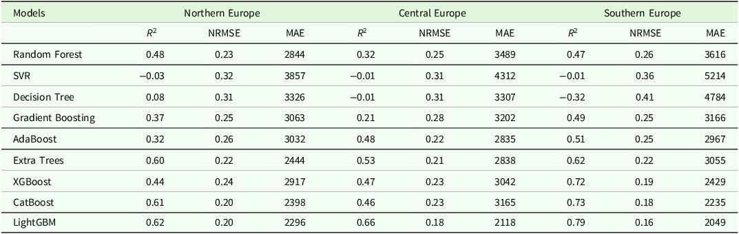
The predictive performance of the tested ML models was evaluated for three major European regions, including Northern, Central, and Southern Europe, based on detrended long-term potato yield data and teleconnection indices. The LightGBM consistently outperformed other models across all regions, as demonstrated by the highest R 2 values and the lowest error metrics. The performance was assessed using four evaluation indicators: the R 2, NRMSE, MAE, and MBE. A comprehensive summary of model performance across all regions is presented in Table 2, and regional prediction accuracy is visualized in Figure 2.
Machine learning models’ performance across the regions

Table 2. Long description
A table comparing the performance of various machine learning models across Northern, Central, and Southern Europe. The table has 10 rows and 9 columns. Column headers are Models, R^2 Northern Europe, NRMSE Northern Europe, MAE Northern Europe, R^2 Central Europe, NRMSE Central Europe, MAE Central Europe, R^2 Southern Europe, NRMSE Southern Europe, MAE Southern Europe. Row labels are Random Forest, SVR, Decision Tree, Gradient Boosting, AdaBoost, Extra Trees, XGBoost, CatBoost, LightGBM. Row 1: Random Forest, 0.48, 0.23, 2844, 0.32, 0.25, 3489, 0.47, 0.26, 3616. Row 2: SVR, -0.03, 0.32, 3857, -0.01, 0.31, 4312, -0.01, 0.36, 5214. Row 3: Decision Tree, 0.08, 0.31, 3326, -0.01, 0.31, 3307, -0.32, 0.41, 4784. Row 4: Gradient Boosting, 0.37, 0.25, 3063, 0.21, 0.28, 3202, 0.49, 0.25, 3166. Row 5: AdaBoost, 0.32, 0.26, 3032, 0.48, 0.22, 2835, 0.51, 0.25, 2967. Row 6: Extra Trees, 0.60, 0.22, 2444, 0.53, 0.21, 2838, 0.62, 0.22, 3055. Row 7: XGBoost, 0.44, 0.24, 2917, 0.47, 0.23, 3042, 0.72, 0.19, 2429. Row 8: CatBoost, 0.61, 0.20, 2398, 0.46, 0.23, 3165, 0.73, 0.18, 2235. Row 9: LightGBM, 0.62, 0.20, 2296, 0.66, 0.18, 2118, 0.79, 0.16, 2049.
Abbreviations: R 2, coefficient of determination; NRMSE, normalized root mean square error; MAE, mean absolute error; SVR, support vector regression; AdaBoost, Adaptive Boosting; XGBoost, eXtreme Gradient Boosting; CatBoost, Categorical Boosting; LightGBM, Light Gradient Boosting Machine.
Regional division of European potato cultivation areas.

Comparison of predicted and actual potato yield in (a) Southern, (b) Central, and (c) Northern Europe. R 2, coefficient of determination; NRMSE, normalized root mean square error; MAE, mean absolute error; MBE, mean bias error. Yield and error values are expressed in kg/ha.

Within the Northern region, LightGBM, with an R 2 of 0.62, demonstrates the model’s strong performance under colder conditions (Table 2). The model also showed relatively low NRMSE (0.20), MAE (2296), and MBE = −1061 (Figure 2c), especially considering the considerably cold climate typical of northern Europe. CatBoost (R 2 = 0.61) and Extra Trees (R 2 = 0.60) followed closely, while the SVR and Decision Tree models exhibited poor performance, as evidenced by low R 2 values and excessively high error rates.
For the Central region, LightGBM once again exhibited the best performance, with R 2 value of 0.66, demonstrating strong predictive power (Table 2). Besides, its corresponding NRMSE of 0.18 indicated low levels of predictive errors. The MAE and MBE values of 2118 kg/ha and −473 kg/ha, respectively, further confirmed that LightGBM provided the most reliable estimates of potato yield in this region (Figure 2b). In comparison, other models, such as XGBoost and CatBoost, did not exhibit better performance, with R 2 values of 0.469 and 0.464, respectively, and higher errors across all metrics. Models such as SVR and Decision Tree yielded negligible or negative R 2 values, indicating limited reliability (Table 2).
The South region, with an R 2 of 0.787, showed the highest model performance across all regions, likely due to greater climatic predictability (Figure 2a). This was supported by an NRMSE of 0.16, reflecting high accuracy in yield prediction, and an MAE of 2049, the lowest among all tested models. Although LightGBM outperformed all models, the better performance of XGBoost and Extra Trees in the southern region also demonstrates the ability to recognize complex, nonlinear relationships regarding climate-vegetation dynamics (Table 2).
These findings underscore the strength of ensemble-based tree models, particularly LightGBM, in capturing complex teleconnection–yield dynamics, with regional differences likely driven by climatic variability, growing season length, and teleconnection signal strength.
SHAP analysis
SHAP analysis for North Region
To enhance the interpretability of the best-performing model (LightGBM), the importance of the most impactful teleconnection indices on potato yield in the northern region was estimated using the SHAP approach. The feature importance ranking, feature interaction plot generation, and force plot generation were analyzed to better interpret the contribution of each teleconnection to variance in yield.
The SHAP feature importance ranking (Figure 3a) identifies EA 8 (East Atlantic in August of the harvest year) and EA/WR 6 (East Atlantic/West Russia in June of the harvest year) as the most dominant predictors of potato yield. The presence of these indices underscores the crucial role of atmospheric circulation patterns in influencing agricultural productivity in Northern Europe. Additionally, lagged teleconnection indices, such as EA (−2) 8 (East Atlantic two years before harvest in August) and EA (−1) 7 (East Atlantic one year prior to harvest in July), exhibit substantial contributions, suggesting long-term climatic memory effects on potato yield. EA (−1) 8 and WP (−2) 8, respectively, are also other important teleconnections after the mentioned ones.
Key teleconnection drivers of potato yield in Northern Europe: (a) SHAP importance ranking, (b) SHAP-value distribution, and (c) individual force plot analysis for a predicted yield, f(x), of 26 876 kg/ha. SHAP, SHapley Additive exPlanations; EA, East Atlantic; EA/WR, East Atlantic/West Russia; WP, West Pacific; PNA, Pacific/North American; SCA, Scandinavia; POL, Polar/Eurasia; AO, Arctic Oscillation; EP/NP, East Pacific/North Pacific; IOD, Indian Ocean Dipole; NAO, North Atlantic Oscillation; SOI, Southern Oscillation Index; PDO, Pacific Decadal Oscillation; MJO, Madden–Julian Oscillation. Niño1 + 2, Niño3, Niño3.4, and Niño4 denote sea-surface temperature indices for the corresponding equatorial Pacific regions. A number following an index denotes the month, and (−1) or (−2) denotes one or two years before harvest, respectively. In panel (c), the horizontal axis is model output in kg/ha; the base value is the expected model output, f(x) is the predicted yield, and red and blue contributions increase and decrease the prediction, respectively.

Figure 3. Long description
Panel A: A vertical bar graph displays the SHAP importance ranking of various teleconnection drivers. The horizontal axis represents the importance score, while the vertical axis lists the teleconnection drivers. Panel B: A scatter plot shows the SHAP-value distribution for the same teleconnection drivers. The horizontal axis represents the feature value, and the vertical axis lists the teleconnection drivers. The colors indicate high and low values. Panel C: A horizontal bar graph with arrows illustrates the individual force plot analysis for a predicted yield of 26,876 kg/ha. The horizontal axis represents the model output in kg/ha, with the base value and predicted yield marked. Red and blue arrows indicate contributions that increase and decrease the prediction, respectively.
The SHAP summary plot (Figure 3b) provides an overall graphical representation of the relative contributions of the most significant teleconnections to the yield forecasts. The x-coordinate value of the plotted points indicates the strength of influence each teleconnection has on the yield forecasts, where points farther from zero indicate a more substantial impact. Color labeling (red and blue) assigned to these points suggests the feature’s relative strength, where high-value points for the teleconnection index are labeled in red and and lower-value points are labeled in blue. The range observed for each teleconnection shows that the influence of each teleconnection index is not fixed but varies relative to its strength and interaction with other teleconnection indices. For instance, EA 8 appears in three distinct groups of points, suggesting different levels of influence on potato yield prediction from this index. This variability may be linked to regional differences in how EA 8 impacts temperature and precipitation in addition to its interactions with other climatic patterns.
Additionally, for the five most important teleconnections (EA 8, EA/WR 6, EA (−2) 8, EA (−1) 7, EA (−1) 8), the presence of multiple groups of points implies that these teleconnections influence yield through varied climatic mechanisms, depending on the strength and phase of the relevant indices. The wider distribution exhibited by some indices, such as EA (−1) 8 and WP (−2) 8, suggests that their impacts on yield are highly complex and likely involve interactions with other climatic variables. Furthermore, the lagged indices (i.e., EA (−2) 8 and EA (−1) 7) highlight the importance of climatic memory, demonstrating how their earlier values influence the ongoing growing season.
The SHAP force plot is a personalized examination of the strength of the effect of the various teleconnections on the predicted potato yield of 26 876 kg/ha compared to the reference yield. Each variable either increases (red, positive effect) or decreases (blue, negative effect) the predicted yield. The SHAP force plot (Figure 3c) provides a detailed visualization of individual yield predictions, showing how different teleconnections influence whether the predicted potato yield is higher or lower than 26 876 kg/ha. High positive contributions of EA 8, EA (−2) 8, EA (−1) 8, EA (−1) 7, and EA/WR 6 result in a yield increase, while WP (−2) 8 negatively affects predictions of detrended potato yield anomalies.
SHAP analysis for Center Region
A comprehensive SHAP analysis was conducted for the Center region to assess the relative contributions of different teleconnection indices in predicting potato yield.
The SHAP feature importance ranking (Figure 4a) showed that EA 8 (East Atlantic pattern in August of the harvest year) is the most dominant predictor. After EA 8, EA (−2) 8 (East Atlantic pattern in August of the 2 years before harvest year), EA/WR 6 (East Atlantic/West Russia with a 3-month lag), WP (−1) 8 (West Pacific in August of the previous year), and EA (−1) 8 (East Atlantic in August of the previous year), respectively, are the most significant teleconnections which affected the potato yield. Other significant indices include PNA (−1)10, EA (−1) 7, EA (−2) 8, and Nino3(−2) 4, indicating that both recent and multi-year lagged teleconnection patterns exert substantial influence on regional yield variations.
Key teleconnection drivers of potato yield in Central Europe: (a) SHAP importance ranking, (b) SHAP-value distribution, and (c) individual force plot analysis for a predicted yield, f(x), of 31 384 kg/ha. SHAP, SHapley Additive exPlanations; EA, East Atlantic; EA/WR, East Atlantic/West Russia; WP, West Pacific; PNA, Pacific/North American; SCA, Scandinavia; POL, Polar/Eurasia; AO, Arctic Oscillation; EP/NP, East Pacific/North Pacific; IOD, Indian Ocean Dipole; NAO, North Atlantic Oscillation; SOI, Southern Oscillation Index; PDO, Pacific Decadal Oscillation; MJO, Madden–Julian Oscillation. Niño1 + 2, Niño3, Niño3.4, and Niño4 denote sea-surface temperature indices for the corresponding equatorial Pacific regions. A number following an index denotes the month, and (−1) or (−2) denotes one or two years before harvest, respectively. In panel (c), the horizontal axis is model output in kg/ha; the base value is the expected model output, f(x) is the predicted yield, and red and blue contributions increase and decrease the prediction, respectively.

SHAP-based feature interaction analysis
The SHAP summary plot (Figure 4b) explains the variability of the impacts of the teleconnections. Although EA 8 remains the main predictor, the classification into different groups for EA (−2) 8 and EA (−1) 8 explains the varying impacts under different climatic conditions. In comparison to the North, Central Europe has wider distributions for EA/WR 6, PNA (−1)10, and Nino3 (−2) 4, showing more variability of their impacts.
The SHAP force plot (Figure 4c) further dissects yield variability, illustrating that EA 8, EA (−2) 8, and EA/WR 6 are the most positively contributing features in increasing the predicted potato yield value of 31 384 kg/ha, while WP (−1) 8 has negative contributions.
SHAP analysis for South Region
The SHAP analysis for the South region was conducted to determine the key teleconnections influencing potato yield variability in a warmer, Mediterranean climate. Similar to Europe’s northern and central regions, SHAP results showed that EA 8 is identified as the most important feature in potato yield prediction, followed by EA/WR 6, EA (−1) 8, and EA (−1) 7 as the most influential features (Figure 5a). Other significant predictors include EA (−2) 8, Niño4 (−1) 7, and Niño4 7, demonstrating both short-term and long-term climate influences on yield.
Key teleconnection drivers of potato yield in Southern Europe: (a) SHAP importance ranking, (b) SHAP-value distribution, and (c) individual force plot analysis for a predicted yield, f(x), of 23 313 kg/ha. SHAP, SHapley Additive exPlanations; EA, East Atlantic; EA/WR, East Atlantic/West Russia; WP, West Pacific; PNA, Pacific/North American; SCA, Scandinavia; POL, Polar/Eurasia; AO, Arctic Oscillation; EP/NP, East Pacific/North Pacific; IOD, Indian Ocean Dipole; NAO, North Atlantic Oscillation; SOI, Southern Oscillation Index; PDO, Pacific Decadal Oscillation; MJO, Madden–Julian Oscillation. Niño1 + 2, Niño3, Niño3.4, and Niño4 denote sea-surface temperature indices for the corresponding equatorial Pacific regions. A number following an index denotes the month, and (−1) or (−2) denotes one or two years before harvest, respectively. In panel (c), the horizontal axis is model output in kg/ha; the base value is the expected model output, f(x) is the predicted yield, and red and blue contributions increase and decrease the prediction, respectively.

Figure 5. Long description
Panel A: A vertical bar graph displays the SHAP importance ranking of various teleconnection patterns. The horizontal axis represents the importance score, while the vertical axis lists the teleconnection patterns. Panel B: A scatter plot shows the SHAP-value distribution for each teleconnection pattern. The horizontal axis represents feature values, and the vertical axis lists the teleconnection patterns. The color gradient from blue to red indicates low to high feature values. Panel C: A horizontal line graph with arrows illustrates the individual force plot analysis for a predicted yield of 23,313 kg/ha. The horizontal axis represents the model output in kg/ha, with the base value and predicted yield marked. Red arrows indicate contributions that increase the prediction, while blue arrows indicate contributions that decrease the prediction.
The SHAP summary plot (Figure 5b) shows the distribution effect of teleconnection indices on potato yield forecasts in Southern Europe. EA 8 continues to be the most dominant teleconnection, followed by EA/WR 6 and several lagged EA indices (EA (−1) 8, EA (−1) 7, and EA (−2) 8), once again confirming the leading influence of North Atlantic variability. In contrast with the northern and central parts, where the influence of EA indices is more dispersed, the southern part of the country has a comparatively concentrated clustering of points, indicating a more stable and direct effect of these teleconnections on yield results. The presence of multiple point clusters for the most highly ranked teleconnections, for example in EA 8 and EA (−1) 8, suggests that varying magnitudes of these indices have varying effects on yield predictions.
The SHAP force plot (Figure 5c) provides deeper insights into individual predictions, illustrating how various teleconnections drive deviations from baseline yield estimates. Results show that EA 8, EA (−1) 8, and EA (−2) 8 are among the most influential teleconnections, highlighting the impact of these periods on potato yield increases. Additionally, EA/WR 6 has a smaller but still positive effect, whereas negative impacts are associated with Nino4 (−1) 7.
Discussion
ML models in agricultural yield forecasting
The results of this study demonstrate that LightGBM consistently outperformed other ML models in predicting potato yield across Europe’s North, Central, and South regions, confirming its status as a state-of-the-art algorithm for complex agricultural forecasting. Generally, all gradient boosting models in European regions have yielded relatively good results, and these findings align with previous studies that have demonstrated the effectiveness of gradient boosting methods for agricultural yield prediction (Chen and Guestrin, Reference Chen and Guestrin2016; Ke et al., Reference Ke, Meng, Finley, Wang, Chen, Ma, Ye and Liu2017). However, aligned with our results, recent research indicates that LightGBM offers superior predictive accuracy and efficient handling of high-dimensional data, especially in agricultural applications (Bhatt and Varma, Reference Bhatt and Varma2023; Jaichandran et al., Reference Jaichandran, Krishna, Arigela, Raman, Dharani and Kumar2022; Parganiha et al., Reference Parganiha and Verma2024; Wang et al., Reference Wang, Wang, Tansey, Liu, Delaney and Quan2025). Our results show that LightGBM’s superior performance can be attributed to its ability to handle large datasets efficiently, capture complex nonlinear relationships, and optimize feature selection through leaf-wise tree growth strategies, which in this research has performed well in exploring three years of lagged teleconnection predictors for potato yield prediction due to its efficient handling of high-dimensional data. Among competing models, Extra Trees, XGBoost, and CatBoost also performed well but were consistently outperformed by LightGBM, while the SVM and Decision Tree were the worst models.
The results in yield prediction varied across regions. In the North, characterized by shorter growing seasons and high climatic variability, LightGBM achieved an R 2 of 0.62, reflecting its robustness in capturing complex climate–yield interactions where teleconnections exert strong influences on temperature and precipitation variability (Olesen et al., Reference Olesen, Trnka, Kersebaum, Skjelvåg, Seguin, Peltonen-Sainio, Rossi, Kozyra and Micale2011; Trnka et al., Reference Trnka, Olesen, Kersebaum, Skjelvåg, Eitzinger, Seguin, Peltonen-Sainio, Rötter, Iglesias, Orlandini, Dubrovský, Hlavinka, Balek, Eckersten, Cloppet, Calanca, Gobin, Vučetić, Nejedlik, Kumar, Lalic, Mestre, Rossi, Kozyra, Alexandrov, Semerádová and Žalud2011). The Central region, benefiting from moderate climatic conditions and a longer growing season, exhibited improved predictive accuracy (R 2 = 0.66). The increased accuracy suggests that teleconnections play a more stable role in shaping potato yield, as also noted in prior agronomic studies (Raymundo et al., Reference Raymundo, Asseng, Robertson, Petsakos, Hoogenboom, Quiroz, Hareau and Wolf2018; Zabel et al., Reference Zabel, Müller, Elliott, Minoli, Jägermeyr, Schneider, Franke, Moyer, Dury, Francois, Folberth, Liu, Pugh, Olin, Rabin, Mauser, Hank, Ruane and Asseng2021). The South region demonstrated the highest predictive performance (R 2 = 0.79). The long and warm growing season in the South provides more consistent weather patterns, reducing the impact of extreme climatic events and making yield prediction more reliable (Olesen et al., Reference Olesen, Trnka, Kersebaum, Skjelvåg, Seguin, Peltonen-Sainio, Rossi, Kozyra and Micale2011). Nevertheless, despite the South’s highest prediction accuracy, it recorded the lowest potato yield levels, emphasizing the complex interplay between climate predictability and heat and water-related stress limiting production. This apparent contrast suggests that higher predictive skill does not necessarily indicate more favorable production conditions. Rather, it may reflect a stronger and more coherent climate limitation on yield variability in southern Europe. In this region, potato production is more exposed to heat stress, seasonal water scarcity, and irrigation dependence, meaning that large-scale climate signals may translate more consistently into yield anomalies. Thus, the South may be more predictable because climate constraints are stronger, while its lower yield level reflects structural limitations related to water availability, heat exposure, and adaptation capacity. Meanwhile, the Center region has the highest yield values, while the North has similar but slightly lower yield values compared to the Center. Warmer temperatures in the South and heat stress may result in potato yield reduction. On the other hand, another reason for lower yield productivity in southern Europe is its reliance on irrigation and greater dependency on water availability (Monaghan et al., Reference Monaghan, Daccache, Vickers, Hess, Weatherhead, Grove and Knox2013; Raymundo et al., Reference Raymundo, Asseng, Robertson, Petsakos, Hoogenboom, Quiroz, Hareau and Wolf2018). These findings have important implications for regional food security and emphasize that predictive skill alone must be coupled with targeted adaptation strategies to secure stable crop production.
Regional variability in teleconnection influence on potato yield predictions
Across all regions, EA and EA/WR patterns emerged as dominant predictors, highlighting the strong influence of North Atlantic atmospheric variability on European agriculture, which aligns with previous studies (Cardil et al., Reference Cardil, Rodrigues, Tapia, Barbero, Ramírez, Stoof, Silva, Mohan and de-Miguel2023; Ionita, Reference Ionita2014; Lim, Reference Lim2015). Specifically, EA 8 was the most significant teleconnection across all regions, highlighting the importance of this feature in potato yield production in Europe. Beyond EA 8, other lagged features of the EA teleconnection (including EA (−1) 7, EA (−1) 8, and EA (−2) 8) also play important roles in all the regions, although the ranking of each one varied across different regions, which aligns with other studies that highlight the high impact of the EA pattern on European agriculture through its strong effect on temperature and precipitation across Europe (Comas-Bru and McDermott, Reference Comas-Bru and McDermott2014; Ionita et al., Reference Ionita, Nagavciuc, Kumar and Rakovec2020; Ossó et al., Reference Ossó, Sutton, Shaffrey and Dong2018; Wulff et al., Reference Wulff, Greatbatch, Domeisen, Gollan and Hansen2017). The dominance of August EA across the three regions may be explained by both climatological and biological mechanisms. Climatologically, the EA pattern is linked to European summer temperature and precipitation variability (Zampieri et al., Reference Zampieri, Toreti, Schindler, Scoccimarro and Gualdi2017), which can influence drought, heat stress, and water availability. Biologically, August often overlaps with tuber bulking, late canopy activity, or final yield formation in many European potato systems. During this period, potato yield is highly sensitive to water deficit and high temperature because these stresses can reduce photosynthesis, accelerate senescence, and limit tuber growth. Therefore, August EA may act as a large-scale indicator of atmospheric conditions affecting one of the most yield-sensitive periods of potato development. However, the exact phenological interpretation differs among regions because planting dates and growing season calendars vary between Northern, Central, and Southern Europe.
West et al. (Reference West, Quinn and Horswell2022) demonstrated that EA plays a significant role in drought control, which has a strong impact on irrigated agricultural fields. As many of the potato fields in southern Europe rely on irrigation, the impact of EA in this area could be explained by the effect of this teleconnection on water availability, which confirms the results of Craig and Allan (Reference Craig and Allan2022), who declare that an increase in EA can cause a decrease (increase) in precipitation in southern (northern) Europe. On the other hand, and in contrast to our findings, Guimarães Nobre et al. (Reference Guimarães Nobre, Hunink, Baruth, Aerts and Ward2019) indicated that EA has a weak effect on the precipitation of southern Europe (Spain) and, consequently, on crop production.
The second most important teleconnection was EA/WR 6, which plays a crucial role in predicting potato yield across all European regions. This result is confirmed by the study of Haslinger et al. (Reference Haslinger, Hofstätter, Kroisleitner, Schöner, Laaha, Holawe and Blöschl2019), who noted that one of the most common reasons for spring drought is EA/WR, due to the large-scale teleconnection’s effect on precipitation. Similarly, our results align with those of Guimarães Nobre et al. (Reference Guimarães Nobre, Hunink, Baruth, Aerts and Ward2019), who stated that EA/WR from May to July and EA averages from June to August are the most frequently used predictors of sugar beet production in large areas of Europe. Notably, SHAP analysis revealed that EA/WR 6 had its strongest influence in the North, aligning with its well-documented impact on Scandinavian precipitation patterns (Ionita, Reference Ionita2014). Additionally, in all European regions, the different effects of ENSO (especially Nino4 and Nino3) were among the top 10 most significant teleconnections.
The multi-year lagged effects of these indices suggest that climate memory plays a crucial role in shaping long-term agricultural productivity. These effects may arise because teleconnections influence temperature, precipitation, and soil moisture (García-Herrera et al., Reference García-Herrera, Paredes, Trigo, Trigo, Hernández, Barriopedro and Mendes2007), while the current results show that many lagged indices are among the most important features in the predictive models. Furthermore, although other short- or long-term teleconnections may not rank among the five leading predictors in every region, their collective contributions remain important to regional model predictions.
The lower predictive accuracy in the north suggests that the strong influence of teleconnections, such as EA and EA/WR, may be negatively impacted by extreme climatic fluctuations and frosts. This, therefore, reduces the validity of yield projections from teleconnection data (Olesen et al., Reference Olesen, Trnka, Kersebaum, Skjelvåg, Seguin, Peltonen-Sainio, Rossi, Kozyra and Micale2011). In contrast, southern Europe exhibited the highest yield predictability, likely due to its relatively stable Mediterranean climate, where teleconnection influences are more consistent and less disrupted by extreme climate fluctuations (Olesen et al., Reference Olesen, Trnka, Kersebaum, Skjelvåg, Seguin, Peltonen-Sainio, Rossi, Kozyra and Micale2011; Raymundo et al., Reference Raymundo, Asseng, Robertson, Petsakos, Hoogenboom, Quiroz, Hareau and Wolf2018).
In addition, results of SHAP Force figures show that while the multi-year lagged EA 8 has the most positive impact on increasing yield, their relative contributions vary by region, with the highest positive impact in the North and South being greater than in the Center. WP was the teleconnection index that had the most negative effect on the Center and Northern regions, although, in the South, Niño4 (−1) 7 played the most negative effect. These regional teleconnection effect differences emphasize the necessity of tailored prediction approaches reflecting growing season length and climatic drivers. It is important to emphasize that the SHAP-based interpretation identifies statistical contributions of teleconnection indices to model predictions rather than causal mechanisms. Although the dominant predictors are consistent with known atmospheric controls on European temperature, precipitation, and drought variability, the present framework should be interpreted as a predictive and diagnostic tool rather than a causal crop-response model.
Implications for climate adaptation and agricultural planning
This study’s findings have direct implications for enhancing European food security by improving early warning and climate adaptation strategies in potato production, a crop vital for nutrition and agriculture. Teleconnection-based prediction can be operationalized through seasonal-to-interannual agricultural early-warning systems. For example, monitoring key indices such as EA, EA/WR, and ENSO-related variables before and during the growing season could support anticipatory decisions on irrigation allocation, planting-date adjustment, cultivar selection, storage planning, and crop insurance risk assessment. At the policy level, such information could be incorporated into regional climate-risk dashboards or agricultural advisory systems to identify years and regions with elevated yield-loss risk (López-Parages and Terray, Reference López-Parages and Terray2022; Martija-Diez et al., Reference Martija-Diez, Rodríguez-Fonseca and López-Parages2022). Similar teleconnection-informed approaches have previously demonstrated potential for seasonal crop forecasting in Europe (Guimarães Nobre et al., Reference Guimarães Nobre, Hunink, Baruth, Aerts and Ward2019).
Long-term climate monitoring of lagged teleconnection effects supports optimized planting calendars, irrigation scheduling, and cultivar selection, especially in drought-prone Mediterranean zones where ENSO signals could guide anticipatory actions for water scarcity (Zampieri et al., Reference Zampieri, Toreti, Schindler, Scoccimarro and Gualdi2017). In Mediterranean regions (South), ENSO-based early warnings could help farmers prepare for drought risks (Bogale and Temesgen, Reference Bogale and Temesgen2021).
Integrating multi-year teleconnection indices into agricultural policies and crop insurance models can improve risk management strategies. Climate-informed crop insurance policies can help mitigate financial losses caused by climate variability (Ceglar & Kajfež-Bogataj, Reference Ceglar and Kajfež-Bogataj2012). Governments could incorporate ML-driven teleconnection forecasts into national agricultural adaptation frameworks (Zabel et al., Reference Zabel, Müller, Elliott, Minoli, Jägermeyr, Schneider, Franke, Moyer, Dury, Francois, Folberth, Liu, Pugh, Olin, Rabin, Mauser, Hank, Ruane and Asseng2021).
Sources of uncertainty and model limitations
While LightGBM demonstrated robust performance in predicting potato yield, several sources of uncertainty warrant consideration. First, the assumption of stationarity in teleconnection–yield relationships may weaken under accelerating climate change, as the strength and spatial patterns of key teleconnections like EA and EA/WR are projected to evolve (Rousi et al., Reference Rousi, Selten, Rahmstorf and Coumou2021; Woollings et al., Reference Woollings, Franzke, Hodson, Dong, Barnes, Raible and Pinto2015). The ML framework does not establish causality. SHAP improves model interpretability by identifying influential predictors, but it does not prove that a given teleconnection directly caused a yield response. Therefore, the results should be interpreted as statistically robust and physically plausible associations rather than direct causal evidence.
Second, data quality introduces uncertainty. The dataset relies on aggregated FAO yield records and large-scale atmospheric teleconnection indices, which may mask local management practices, soil conditions, or reporting inconsistencies across European countries (Lobell et al., Reference Lobell, Thau, Seifert, Engle and Little2015). A key limitation of this approach is that country-level FAO data aggregated into broad European regions cannot fully represent subnational variability and local physical mechanisms in soil conditions, irrigation practices, crop varieties, pest pressure, extreme and compound events, and farm-level management. Therefore, the results should be interpreted as large-scale regional associations rather than field-scale causal relationships. Additionally, teleconnection indices derived from global atmospheric models may oversimplify regional-scale climate impacts relevant to potato phenology (Deser et al., Reference Deser, Hurrell and Phillips2017).
Omitted variables represent an additional source of uncertainty. Irrigation availability, soil water-holding capacity, cultivar selection, pest and disease pressure, fertilizer management, and technological progress may influence potato yield independently of teleconnection variability. Although detrending reduces the long-term influence of technological improvement, it cannot remove all management-related confounding effects.
The deliberate exclusion of direct meteorological variables (temperature, precipitation, soil moisture) focused analysis on teleconnection signals but limits capture of local weather extremes and farm management effects (Comas-Bru and McDermott, Reference Comas-Bru and McDermott2014). While teleconnections like EA and EA/WR indirectly modulate regional climate (Craig and Allan, Reference Craig and Allan2022), this choice avoids multicollinearity but reduces granularity for microclimatic stressors like localized heat stress in Southern Europe (Raymundo et al., Reference Raymundo, Asseng, Cammarano and Quiroz2014; Vicente-Serrano et al., Reference Vicente-Serrano, Lopez-Moreno, Beguería, Lorenzo-Lacruz, Sanchez-Lorenzo, García-Ruiz, Azorin-Molina, Morán-Tejeda, Revuelto, Trigo, Coelho and Espejo2014). Future studies should develop hybrid frameworks that combine teleconnection indices with local hydroclimatic variables and compound-event indicators to better represent causal pathways and crop stress processes while maintaining predictive skill.
Dataset limitations further constrain model scope. The 36-month lag window captures substantial climate memory but may miss decadal oscillations or compound extreme events (e.g., prolonged heatwaves combined with drought or flood) that drive outlier yield losses (Trenberth et al., Reference Trenberth, Dai, Van Der Schrier, Jones, Barichivich, Briffa and Sheffield2014b). The study’s temporal coverage (1961–2023) also omits potential shifts in interdecadal teleconnection variability that could alter future predictability (Ionita et al., Reference Ionita, Caldarescu and Nagavciuc2021).
Conclusion
The current study showed that LightGBM captured nonlinear and lagged associations between major teleconnection patterns and potato yield across northern, central, and southern Europe, achieving R 2 values of 0.62, 0.66, and 0.79, respectively. The East Atlantic and East Atlantic/West Russia patterns, particularly their August values and multi-year lags, were the dominant predictors, indicating a climate-memory signal in regional yield variability. Although the South had the highest predictive skill, it had the lowest historical yield level, likely reflecting heat and water stress, whereas central and northern Europe had higher yield levels but remained sensitive to climate variability and frost. Integrating teleconnection information with interpretable ML can support seasonal-to-multi-year early warning and climate-informed planning, although future work should combine these indices with local climate drivers and evaluate finer spatial scales and additional crops.
Acknowledgments
During manuscript revision, the authors used ChatGPT (OpenAI, GPT-5, https://chatgpt.com; accessed 23 September 2026) solely for English-language editing, including grammatical correction and improvements to wording. The authors reviewed and approved all edits and take full responsibility for the final manuscript.
Author contributions
Mojtaba Naghdyzadegan Jahromi conducted the analyses and wrote the main manuscript. Alireza Gohari contributed to manuscript revisions. Ali Torabi Haghighi supervised the research, provided methodological guidance, and led the overall direction of the study. All authors reviewed and approved the final manuscript.
Funding statement
This research was supported by the FARMWISE project, funded by the European Union under the Horizon Europe call HORIZON-CL6-2023-ZEROPOLLUTION-01 (Grant Agreement No. 101135533), and by Maa- ja vesitekniikan tuki ry (MVTT; Grant No. 44930, BSCANDF project).
Competing interests
The authors declare there are no conflicts of interest.
Ethical standards
Not applicable.



 Open access

