I. INTRODUCTION
Passive device designs must meet the stringent requirements brought about by the continued increase in capabilities and adoption rates of wide band gap power semiconductors. Specifically, magnetic component designs need to consider new operating spaces and to take advantage of new soft magnetic materials and material processing. Generally, power converter controls and topologies are moving toward very high efficiencies through soft switching techniques that greatly reduce the losses associated with the switching devices. This in turn means that a dominant loss component of a power converter will be the passive devices and specifically the magnetic components.Reference Steigerwald, De Doncker and Kheraluwala1–Reference Beddingfield, Storelli and Bhattacharya3 Furthermore, magnetic components will continue to play a critical role in power converters due to their energy storage and isolation capabilities. The high reliability and wide design envelope of magnetic devices also make them critically important elements of any power converter design. It is because of the aforementioned factors that both magnetic design techniques and the components used need to be fully characterized and improved.
Analytical predictions will enable improved screening and optimization of magnetic designs to reduce the number of designs that require careful characterization and more detailed optimization through experimental prototype efforts and/or more computationally intensive applied electromagnetic tools such as finite element-based modeling. Furthermore, analytical expressions can be developed to incorporate new materials and new material processing strategies. By determining estimations for currently unavailable materials or magnetic cores, this approach can also help to guide the research and development goals for new alloy development as well as advanced manufacturing process optimization techniques. That is, the magnetic core research and development can be refocused on the realization of a subset of candidate designs that have shown promise through analytical expressions and have been confirmed by finite element modeling techniques. Such an approach is particularly useful in understanding the role and performance potential of magnetic cores that are post-processed with strain annealing techniques in which the permeability can be readily tuned along the length of the ribbon. The utility of an analytical design approach is in determining which strain annealing profiles are most useful such that the material and process development can focus on optimized designs. Similarly, the analytical approach can better define what baselines provide a meaningful comparison.
Due to the myriad of factors that influence the design of a power electronics converter, it is important to characterize and provide predictions for magnetic designs using similar methodologies to that of semiconductor device characterizations. That is, magnetic devices need to be characterized for all operational sensitivities, e.g., temperature, loading, dV/dt, etc. in a particular solution space.Reference Beddingfield and Bhattacharya4 This research focuses on two of the more influential aspects of magnetics design, namely the direct relationship between the local temperature rise and core magnetizing losses. It is noted that for some power electronics converter designs leveraging amorphous and metal amorphous nanocomposite (MANC) ribbon-based core materials, additional loss contributions have been determined to be significant and even dominant in some cases as a result of eddy current losses generated within the ribbon plane due to flux leakage from the magnetic core. While we do not specifically discuss that the source of losses in this work, similar techniques are relevant to address those challenges and are the subject of on-going research activities. It is also important to note that new post-processing techniques such as strain annealingReference Aronhime, Degeorge, Keylin, Ohodnicki and McHenry5–Reference Kernion, Ohodnicki, Grossmann, Leary, Shen and Keylin10 and field annealing,Reference Ohodnicki, Long, Laughlin, McHenry, Keylin and Huth11 enable new material characteristics. These materials could lead to improved designs and alternative solutions. However, without full characterization and analytical screening of the post-processing dependent performance of these materials, their development is not able to successfully transition into applications and components for which they can have the most significant impact on overall performance. The characterization of magnetic designs and materials under operationally relevant conditions is paramount to continued success and improvements in magnetics design.
This paper will highlight the improved capabilities in power magnetics, component level, performance enabled by the strain annealing post-processing techniques. It will first provide a brief overview of the state of the art as motivation to provide deeper insight into thermal modeling and loss predictions of traditional materials. These loss predictions are strongly coupled to thermal performance and can provide insight for the thermal profile of the magnetic ribbon cores. An observed gradient in temperature is due to the flux density concentration and the anisotropic core. This anisotropy is represented in the proposed thermal model. Finally, an example is explored with a comparison of physical cores designed for high power inductor applications.
II. MOTIVATION
Fully understanding the losses for a magnetic component is critical for optimal design in power electronics applications. It is also important when determining the necessary cooling systems for a particular design. Multiple authors and publications explore the variations in core loss due to the excitation waveform.Reference Jiles and Atherton12–Reference Muhlethaler, Biela, Kolar and Ecklebe15 However, all of these prior investigations base their loss models on assumptions of uniform flux density within the core. These models either use the maximum of average flux density or the overall peak flux density. While this can be useful for predicting the losses as a function of excitation waveforms enforced by the electrical circuit, it does not account for core geometry, flux concentration and pinching, and other material effects. Permeability-engineered cores with significant variations in relative permeability and the resulting flux density profiles will be further susceptible to errors in loss estimations when using the previously mentioned approaches and these modeling approaches cannot provide guidance to the optimal magnetic core designs in cases where permeabilities can be readily adjusted throughout a given magnetic core.
In Ref. Reference Havez16, the author derives and highlights the differences in estimated total losses using the local peak flux density-associated losses against the rational approach using a single global flux density. The solution space explored is useful for small components but does not explore some of the design possibilities that are needed for the high power applications of interest. Similarly, Ref. Reference Cougo17 utilized a similar analysis to recommend variations to the magnetic core cross section. Here the motivation was, as is true in this analysis, minimizing thermal variation over the core profile. Unlike this paper's approach, utilizing variations in effective permeability, the author of Ref. Reference Cougo17 recommended varying heights along the toroid radius. As the author mentions, this is problematic for manufacturability. Furthermore, the author fell short of a complete analysis and did not fully analyze the variation in core losses due to the improved flux density profile. Finally, the author was only able to explore solutions in finite element analysis (FEA). There is ample room for continued analysis and analysis that considers newly proposed post-processing techniques.
A. Flux density definitions
For clarity, it is important to first define the variations in flux density representations. The local flux density is the typical flux density that is derived using the relationship between current and magnetic field using Ampere’s law (1). Typically, the relative permeability, µ, is the product of the constant relative permeability of the core material under investigation, µr, and the permeability of free space, µ0. However, because strain annealing will enable an arbitrarily variable profile of relative permeabilities, it is left as a function of the toroid radius, r, assuming that the permeability varies only as a function of core radius but is otherwise equal along the core height and circumferential direction. Such a permeability profile is readily produced using strain annealing techniques through a monotonic variation in applied tension during the strain annealing process followed by standard core winding and fabrication processing techniques. The flux density is scaled by the number of turns, N, and the excitation current, I, regardless of excitation shape. This flux density is valid in the applicable range of r between the inner radius, r i, and the outer radius, where λ is used to define the ratio between the outer radius and the inner radius. The average flux density in a toroid is shown in (2).
 $${\left. {B\left( r \right) = {{\mu \left( r \right)NI} \over {2\pi r}}} \right|_{{r_{\rm{i}}} \le r \le \lambda {r_{\rm{i}}}}}\quad ,$$
 $${B_{{\rm{avg}}}} = {{NI} \over {{r_{\rm{i}}}\left( {\lambda - 1} \right)2\pi }}\int_{{r_{\rm{i}}}}^{\lambda {r_{\rm{i}}}} {{{\mu \left( r \right)} \over r}} {\rm{d}}r\quad .$$
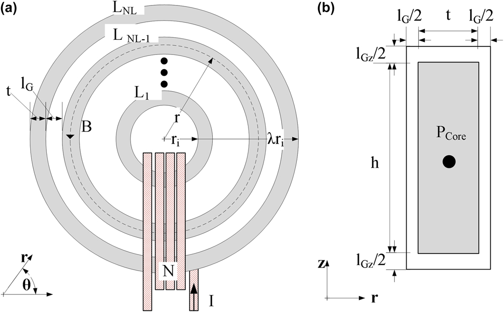
Below in Fig. 1, an example toroid is drawn with the top view and a cutout side view of one of the ribbon layers. This drawing illustrates some of the physical and construction parameters. Similarly, the dimensions shown in this drawing will enable the detailed definition of various thermal impedances as described in Sec. III.
Toroid geometry with dimensions, (a) Top view; (b) Individual ribbon layer cutout view.

B. Thermal management
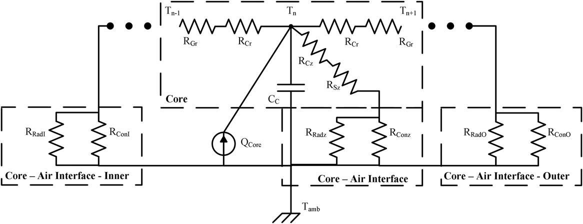
Given the above-defined flux density profiles, a proper thermal model is needed to account for the anisotropic nature of the ribbon wound magnetic cores. A model can be represented as an equivalent circuit of thermal impedances, thermal capacitances and heat flow with resistances, capacitors, and current injections, respectively, as described.Reference Kasap18 Other researchers have followed a similar approach of modeling power magnetics by either using isotropic materials or averages of bulk materials, Refs. Reference Odendaal and Ferreira19 and Reference Hilal, Raulet and Martin20. In Ref. Reference Das, Wei, Vaisambhayana, Cao, Tian, Tripathi and Kjær21, the authors model anisotropic cores but do not consider variations in heat injection due to a flux density profile. To account for this localized heat injection due to localized losses, it is necessary to have a localized thermal model. This proposed model is shown below in Fig. 2. This model discretizes the spiral of a wound magnetic tape into several concentric ring layers of one ribbon thickness. The subscript n is the discretization variable. Each ring has a thermal capacitance, C c, corresponding to its effective ring mass and material’s specific heat capacity. However, this capacitance needs only be considered for thermal transients. At steady-state temperatures, the thermal mass capacitance can be neglected. The heat injected is directly attributed to the local losses, represented by the current injection P core.
2D thermal model for anisotropic magnetic ribbon cores.

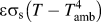
To define the above model, the heat flow processes of convection and radiation are also treated as impedances of the form shown in (3). The components of (3) for all of the thermal impedances of Fig. 2 are described in Table I.
 $$R = {l \over {a{k_{\rm{t}}}}}\quad .$$
Description of thermal impedances for anisotropic core model.

Values for constants, easily found in various textbooks and research studies, are presented from Refs. Reference Laaidi, Belattar and Elbaloutti22–Reference Leary, Ohodnicki and McHenry24. The core is assembled of N L layers such that R n is the radius at the center of a ribbon of the nth layer. The G region is the gap between two ribbon layers and t is the thickness of a ribbon layer. The dimension l G can also be used to account high thermal impedance materials between ribbon layers and between the ribbon and air. This can be used to represent thin oxidation layers or epoxies. The radial G effect can be estimated by using the thermal impedance of air, oxidation, or epoxy with the core fill factor. High fill factors would have low G region impedances while low fill factor cores would have a high anisotropy in the tangential and radial dimensions. The thermal anisotropy varies significantly with the bulk magnetic core fill factor. The ratio of thermal conductivity between the tangential and radial directions of toroid is shown in (4), where F, the fill factor, is the ratio of the core thickness, t, and the sum of the ribbon thickness and the gap thickness, G. This ratio can be near five for typical fill factors, around 80–85%, ribbon thicknesses, and fill materials. This assumes that the ribbon and G region have thermal constant conductivities of k c and k G, respectively.
 $${{{k_{\rm{t}}}} \over {{k_{\rm{r}}}}} = {{\left( {{k_{\rm{G}}}G + {k_{\rm{c}}}t} \right)\left( {{G \over t} + {{{k_{\rm{G}}}} \over {{k_{\rm{c}}}}}} \right)} \over {\left( {G + t} \right)\left( {{{{k_{\rm{G}}}G} \over t} + {k_{\rm{G}}}} \right)}} = {F^2}\left( {2 - {{k_{\rm{c}}^2 + k_{\rm{G}}^2} \over {{k_{\rm{c}}}{k_{\rm{G}}}}}} \right) + F\left( {{{k_{\rm{c}}^2 + k_{\rm{G}}^2} \over {{k_{\rm{c}}}{k_{\rm{G}}}}} - 2} \right) + 1\quad .$$
The effective thermal impedance for convection is determined using Newton’s law of cooling. The variation in the k [c/G] value, replacing the traditional symbol h, for the coefficient of convective heat transfer in this impedance is due to the different cooling methods ranging from natural, unforced air, convection to higher performance forced liquid cooling. The thermal impedance modeling radiation utilizes Stefan’s law and reorganizes the law into the form of a typical thermal impedance. In these impedances, T is used to represent the core layer temperature and T amb is used to represent the ambient temperature.
In Fig. 2, the basic model most properly represents interior layers of the ribbon. For the innermost and the outermost layers, a slight modification is needed. Specifically, the model region defined as core–air interface connects to both the z dimension and the radial dimension. These augmentations to the radial thermal impedance account for the convection and radiation associated with the exposed broad surface of the inner and outermost ribbon layers. These are represented by the two-edge regions of core–air interface inner and outer, respectively.
This model is then connected to other radial models to represent the different tangential zones of the magnetics. Three examples of zones are uncovered, covered with heat sink material, and covered with heat injection components. The above model without any modifications can represent uncovered zones. The two covered zones both affect the z dimension thermal resistances and while a zone covered with the heat injection component could potentially add to the heat injection. That is, a heat sink material adds its own thermal model between the edge, inner, or outer impedances depending on its physical connection to the core. Alternatively, a heat injection component has several aspects to consider for complete thermal modeling. A prime example of a potential external heat injection component is the excitation coils in a magnetic component. One of the simplest modifications is modeling the use of a thermal insulator between the excitation coil and core. With this scenario, the affected region does not have significant heat flow paths to ambient and thus all model connections to the sink can be removed. However, if a thermal conductor is used, one must consider the heat injection caused by the heating of the excitation winding. The thermal path from the core to the thermally conductive bobbin to the excitation coil does have a path to free space and thus the thermal resistances to ambient of convection and radiation can be included.
With a complete thermal model of the transformer, we can see that the local loss profile has a significant impact on the temperature profile of the core. The thermal anisotropy between the radial and tangential dimensions further couples the temperature profile to the local losses. Where the thermal body be isotropic, the temperature profile would normalize somewhat but still be heavily dependent on the heat injection profile. The thermal impedances in the z dimension have some variations between the layers due to varying surface areas but it is minimal. The exception to this trend is the innermost and the outermost layers and the layers where the broad surfaces are exposed to ambient temperatures. Thus, the radiative and convective impedances at these two layers allow significant heat flow and ultimately a steady-state temperature nearer to ambient. This affects closely adjacent layers due to the larger temperature difference.
C. Heating impact
The heating of the core has several impacts. The core must remain below certain temperatures, e.g., the Curie or impregnated epoxy breakdown temperatures, with safety margins that would affect fundamental core properties. However, in most practical power magnetic designs, there are even lower critical temperatures that are important to avoid such as the thermal limits of insulating epoxies or plastics.
While these limits exist, one may wish to have designs that further limit the maximum core temperature. The temperature impacts on the operating performance of cores are generally material specific withReference Ridley and Nace25 providing some polynomial approaches to account for the variations in ferrites. An example of a ferrite material that has a wide range of variation due to heating is L material.26 Nearly all performance metrics have varying sensitivities to operating conditions including permeability, core loss, and saturation flux density. While ferrites have shown this variability, it is not always the case for nanocrystalline.Reference Beddingfield and Bhattacharya4 In that study, cores were shown to have minimal variation in measured core losses over a reasonable temperature range. However, the effective relative permeability of the core changed significantly. In operating up to 80 °C, the effective relative permeability of the core dropped roughly 300%. This resulted in a much lower transformer magnetizing inductance. In a practical converter, this could result in up to a 9-fold increase in conduction losses because of a three-time increase in the required magnetizing current. This increase in current would also have to be accounted for in determining the system maximum current rating and the selection of winding gauge. However, this increase in magnetizing current could be used advantageously as certain converters utilize magnetizing current to increase the window for which semiconductor switching losses are minimized. The authors in Refs. Reference Xuewei, Prasanna and Rathore27 and Reference Kheraluwala, Gascoigne, Divan and Baumann28 showed that the how so-called soft switching of converters could utilize magnetizing current for improved operation. Thus, regardless of the design, it is important to have a firm grasp of the overall operating temperature and to understand the implications that this temperature has on the magnetic core performance.
III. STRAIN ANNEALING PROFILES
As mentioned above, applying mechanical strain as a post-production process to the magnetic ribbon causes variations in the relative permeability. By applying an arbitrary strain profile along the length of the ribbon, a core with an arbitrary relative permeability between various layers of ribbon in the radial direction can also be manufactured. While the ultimate profile achievable could be arbitrary, four fundamental profiles are presented here for their logical and practical utility as well as their manufacturability during the strain annealing process without the need for highly sophisticated process controls. These profiles are constant strain, ramped strain, ramped strain with initial strain, and exponential strain. These profiles will be discussed further in detail in the respective subsections. In this analysis, there are a myriad of variables to explore and potentially many local inflection points in relative performance. As such, this analysis is meant to provide an initial overview and to allow further in-depth study for specific cases. For all of the presented design cases, the core permeance was held to be the same. In this way, the comparison of strain annealing approaches is for magnetic devices with the same inductance, as inductance is equal to the permeance times the turns squared. Each strain annealing profile is analyzed to present the average flux density, permeance, loss estimation based on the average flux density, the heat injection, and finally the loss calculation based on the local flux density.
The profiles are presented in terms of the core radius to easily apply the proposed permeability to the definition of flux density. However, this radially defined profile does not provide insight into the strain profile. For this, we must determine the length along the ribbon for which the strain should be applied. While the toroid is constructed as an Archimedean spiral, a simplified approximation yields adequate results. The length function is then presented in (5). The layer number, L n, is determined by (6). Once a desired permeability profile is chosen, the length for which the strain should be applied, l r, given a desired radius location, r, is easily determined in (7).
 $${L_{\rm{r}}} = \pi {L_{\rm{n}}}\left( {2{r_{\rm{i}}} + {t \over F}\left( {{L_{\rm{n}}} - 1} \right)} \right)\quad ,$$
 $${L_{\rm{n}}} = {{F\left( {r - {r_{\rm{i}}}} \right)} \over t}\quad ,$$
 $${l_{\rm{r}}} = \pi \left( {{{F{r^2}} \over t} - {{Fr_{\rm{i}}^2} \over t} - r - {r_{\rm{i}}}} \right)\quad .$$
A. Assumptions used in analysis
As with any numerical analysis and modeling of physical systems, certain assumptions must be made. There are three primary assumptions used in this analysis. The first is that the loss term, β, does not change with the strain and permeability or temperature. Future work will verify this assumption or provide functions and curves to account for the impact. The initial samples under investigation have not shown significant variations. Another simplification is that the core height, h, or strain-annealed ribbon width is constant. While applying strain, the ribbon stretching causes elongation in the axis of the applied strain and shrinkage in the other axes. This can result in a reduction of the thickness of the ribbon and the width of the ribbon. The cross sectional area is consequently reduced. This could lead to a slightly higher flux density than predicted flux density in the ribbon required due to the reduced area. The third assumption is that the magnetic and electric properties of the core material will not change with temperature. While it has been shown to have significant effects,Reference Beddingfield and Bhattacharya4 incorporating the full impact requires a specific core thermal model. Furthermore, the initial core parameters will remain sufficiently unaffected while the core temperatures remain low. It is with the understanding of the variations and the assumptions that the forthcoming analysis remains adequate for the understanding of strain annealing effects on the total core losses of a finished magnetic core. For this analysis, the loss term and the ribbon width, core height, and thickness terms were assumed constant and unvarying with temperature.
In the forthcoming analysis, the relative permeability, scaled by the permeability of free space, µ0, is represented by µ. The subscript denotes the type of the strain annealing profile. The differential volume of the toroid reduces to the circumference at that radius multiplied by the differential radius volume. The ratio between inner radius, r i, and outer radius is denoted with λ. As shown in Ref. Reference Aronhime, Degeorge, Keylin, Ohodnicki and McHenry5, a set of Steinmetz parameters k, α, the frequency, f, and loss component, β, can be used to fit the loss curves for an arbitrary excitation using (8). The authors in Ref. Reference Beddingfield, Vora, Storelli and Bhattacharya29 showed how a map or surface of measured losses could be fitted using (8) for several common excitation waveforms. In the following analysis, accurate parameters are assumed to have been measured and fitted. The scaling factor, k, has a wide range of values and can be used to modify the equation to handle parameters extracted for either 1000’s of Hz or kHz. In other words, k, could be different by a factor of 1000α depending on if frequency, f, is analyzed in Hz or kHz. The frequency factor, α, is typically in the range of 1–3 while the flux density term, β, is between 2 and 3.
 $${P \over V} = k{f^\alpha }{B^\beta }\quad .$$
The Steimetz fittings are often further expanded to consider loss partitioning in terms of different operative mechanisms.Reference Steinmetz30 An alternate loss model, emphasizing loss separation, is the 3-term Steinmetz equation that is expressed using scalars k hys, k eddy, and k exc which are used to partition power loss density per unit volume for (i) hysteresis, (ii) classical eddy current, and (iii) excess loss components, respectively.
In the product literature, it is common to lump the last two terms as total eddy current losses with a power law exponent α dependent on induction. Static hysteresis loss dominates at low frequencies and eddy currents dominate at high frequencies.
The partitioning constant, k eddy, is proportional to the square thickness of the material and inversely proportional the material’s resistivity. Therefore, high resistivity is desired for magnetic components operating at high AC frequencies. While the resistivity of amorphous metal ribbons (AMRs), MANCs, and crystalline materials are tunable with chemistry, the resistivity of AMRs is typically are 2–3 times larger which significantly reduces eddy current losses. Hysteretic losses are diminished in AMR, MANCs, and bulk amorphous materials through random magnetic anisotropy.Reference Herzer and Buschow31 Typically, magnetic induction is sacrificed for glass forming ability (and resistivity) in AMR and bulk amorphous alloys as compared with crystalline materials, e.g., Si steels. MANCs offer a middle ground between the highest inductions of crystalline materials and high resistivity of amorphous materials. The ability to cast AMR’s and MANCs in thin cross sections significantly impacts eddy current losses to reduce high-f losses.Reference Herzer and Buschow31
The anomalous eddy current (AEC) losses, third term in the three-term Steinmetz equation is associated with dynamic domain wall motion. AEC contributions originate at a mesoscale due to local heterogeneities in the magnetic domain structure.Reference McHenry and Laughlin32,Reference Bertotti33 Just as laser scribing is used in pinning magnetic domain walls in Si steels to limit their dissipation of energy at high frequencies, inducing anisotropy in AMR and MANCs have been used to lower losses at high frequencies. In AMRs, anisotropy is typically induced by transverse (to the AMR length) field annealing, rolling, and more recently strain annealing.Reference Kernion, Lucas, Horwath, Turgut, Michel, Keylin, Huth, Leary, Shen and McHenry34
B. Constant permeability
This strain annealing profile has no profile variation from the permeability of traditional cores. However, reducing the permeability of the core by applying strain could eliminate the need of air gaps or achieve some other specifically desired relative permeability. In this application, a constant strain is applied to the ribbon to result in a constant permeability for the entire ribbon. Thus, the radially dependent permeability is a constant (9). As a wound toroid core, this strain annealing profile would result in a magnetic flux density profile that is like any other core of the same constant permeability. As such, this approach will be used as the baseline for comparison of other strain annealing profiles.
 $$\mu \left( r \right) = {\mu _{\rm{c}}}\quad .$$
By averaging the radially dependent flux density over the boundaries of the core, it is clear that the average flux density is (10), where N is the number of turns in the exciting coil and I is the exciting current. The resulting core permeance,  $\hat{P}$, for a core of height, h, is derived from the flux and is shown in (11). These dimensions can be seen in Fig. 1.
 $${B_{{\rm{avg}}}} = {{NI} \over {2\pi }}{{{\mu _{\rm{c}}}\ln \left( \lambda \right)} \over {{r_{\rm{i}}}\left( {\lambda - 1} \right)}}\quad ,$$
 $$\hat{P} = {\phi \over {NI}} = \int_0^h {\int_{{r_{\rm{i}}}}^{\lambda {r_{\rm{i}}}} {B\left( r \right){\rm{d}}r{\rm{d}}z} = {h \over {2\pi }}{\mu _{\rm{c}}}\ln \left( \lambda \right)\quad .}$$
By using the flux density averaged over the entire core and the total core volume in the Steinmetz loss equation, we can see that the losses based on the average flux density are shown in (12).
 $$P\left( {{B_{{\rm{avg ‐ }}{\mu _{\rm{c}}}}}} \right) = k{f^\alpha }VB_{{\rm{avg}}}^\beta = k{f^\alpha }h\pi r_{\rm{i}}^2\left( {{\lambda ^2} - 1} \right){\left( {{{NI} \over {2\pi }}} \right)^\beta }{\left( {{{{\mu _{\rm{c}}}\ln \left( \lambda \right)} \over {{r_{\rm{i}}}\left( {\lambda - 1} \right)}}} \right)^\beta }\quad .$$
For understanding the heat injection profile, it is useful to investigate the local power loss (13). This is equivalent to the heat injection, Q, in the thermal model. Here the volume is the local slice of volume.
 $${P_{{\rm{loc}}}} = Q = k{f^\alpha }hC\left( r \right)tB{\left( r \right)^\beta } = k{f^\alpha }ht2\pi {r^{1 - \beta }}{\left( {{{{\mu _{\rm{c}}}NI} \over {2\pi }}} \right)^\beta }\quad .$$
Finally, an estimation of the losses using the local flux density is presented in (14). This method of loss calculation applies the Steinmetz equation to small slices of the core. As such, the differential volume is needed. This volume is equivalent to the circumference of the infinitely thin slice and is represented by C(r). The height of the core is a scalar to the volume and is independent of the radius.
 $$P\left( {{B_{{\rm{loc ‐ }}{\mu _{\rm{c}}}}}} \right) = k{f^\alpha }h2\pi {\left( {{{NI} \over {2\pi }}} \right)^\beta }{{\mu _{\rm{c}}^\beta r_{\rm{i}}^{2 - \beta }\left( {{\lambda ^{2 - \beta }} - 1} \right)} \over {2 - \beta }}\quad .$$
With two estimations for losses, one based on the average flux density and the other based on the summation of local losses, a comparison of differences between the two can provide insight into the design cases for which the numerical simplification of using B avg is valid (15). It is important to note that all constant permeability design cases result in less than a 10% variation in estimation. It is only when the ratio between inner and outer radii, λ, is high and the loss term, β, is low that the estimation difference is at its greatest. However, using the average flux density to predict magnetic core losses obfuscates the thermal impacts by considering the losses as a whole and not as a profile. Furthermore, this loss estimation will miss the loss impacts of different strain annealing profiles with the same permeance.
 $${{P\left( {{B_{{\rm{avg ‐ }}{\mu _{\rm{c}}}}}} \right)} \over {P\left( {{B_{{\rm{loc ‐ }}{\mu _{\rm{c}}}}}} \right)}} = {{\ln {{\left( \lambda \right)}^\beta }\left( {{\lambda ^2} - 1} \right)\left( {2 - \beta } \right)} \over {2\left( {{\lambda ^{2 - \beta }} - 1} \right){{\left( {\lambda - 1} \right)}^\beta }}}\quad .$$
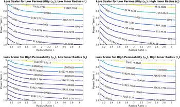
Using (14), loss contours for the general design space for power magnetics can be established. Specifically, the local losses can be studied under four different scenarios. This would be the combination of low and high inner radii and low and high permeability. In this case, the low inner radius is 10 mm and the high inner radius is 100 mm. The relative permeability is chosen with the focus of power inductors where low permeability is generally ideal. In this case, the permeabilities studied are 10µ0 for the low permeability case and 100µ0 for the high permeability case. The values of the contour are loss scalars that reflect division of common variables. These common variables are shown below in (16). For all of the strain annealed permeability profiles, the contours in Fig. 3 will be used as the baseline to compare the impact of a strain annealed induced permeability profile on the toroid’s magnetization losses. These curves show the scalar term of a constant permeability design local loss. In other words, a constant permeability design total loss could be determined by multiplying (16) by a point of the curve corresponding to the chosen design.
 $$k{f^\alpha }h2\pi {\left( {{{NI} \over {2\pi }}} \right)^\beta }\mu _0^\beta \quad .$$
Contours of baseline values for losses of various toroid designs.

A common radius ratio and flux density loss exponent, β, for power magnetics is 2 and 2.4, respectively. At this design point, the loss scalars for the low permeability designs are 959 and 382 for low and high inner radius designs, respectively. The higher inner radius has a lower loss scalar reflecting the lower peak flux density for a given excitation. The high permeability loss scalar for the low inner radius is 2.41 × 10⁵ and 9.59 × 10⁴ for the high inner radius.
C. Linear graded permeability
This permeability is a logical assumption to achieve a flat flux density profile. This is because the permeability increases proportionally to the radially dependent decrease in magnetizing force caused by the increasing magnetic path length at larger radii. Here, the slope of the permeability is chosen as µs. The relative permeability scales only as a function radius and has no effective offset, by the profile definition, a relative permeability that would be zero at a radius of zero if zero relative permeability could exist. The strain should be applied in a stair step fashion with increasing length such that each layer of wound ribbon in the toroid is subjected to the same strain and results in the same permeability over the layer. This profile has the minimum variation between maximum and minimum flux density as they should, within manufacturing tolerances, be the same. The permeability function is shown below in (17).
 $$\mu \left( r \right) = {\mu _{\rm{s}}}r\quad .$$
The average flux density and permeance for a graded permeability profile are shown below in (18) and (19). As mentioned above, the flux density profile is flat such that it is equivalent to the average flux density along the entire core profile. Therefore, the flux density is no longer dependent on the core radius.
 $${B_{{\rm{avg ‐ }}{\mu _{\rm{s}}}}} = {{NI} \over {2\pi }}{\mu _{\rm{s}}}\quad ,$$
 $$\hat{P} = {h \over {2\pi }}{\mu _{\rm{s}}}{r_{\rm{i}}}\left( {\lambda - 1} \right)\quad .$$
The power loss due to the average flux density, (18), is shown below in (20). Again, the basic Stienmetz estimation is used for losses.
 $$P\left( {{B_{{\rm{avg ‐ }}{\mu _{\rm{s}}}}}} \right) = k{f^\alpha }h\pi r_{\rm{i}}^2\left( {{\lambda ^2} - 1} \right){\left( {{{NI} \over {2\pi }}} \right)^\beta }{\mu _{\rm{s}}}^\beta \quad .$$
The local losses are calculated for this profile in (21). It is interesting to note that despite the flat flux density profile, the heat injection profile along the core is not flat. This is because the volume of the core rings has increased in the outer radii.
 $${P_{{\rm{loc ‐ }}{\mu _{\rm{s}}}}} = k{f^\alpha }ht2\pi r{\left( {{{{\mu _{\rm{s}}}NI} \over {2\pi }}} \right)^\beta }\quad .$$
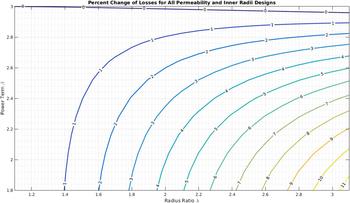
Finally, the total losses, calculated locally, are shown in (22). The percent change in losses is shown below in Fig. 4. In these design comparisons, the slope factor, µs, is chosen to ensure that the linearly graded permeability results in the same core permeance as the constant permeability core permeance.
 $$P\left( {{B_{{\rm{loc ‐ }}{\mu _{\rm{s}}}}}} \right) = k{f^\alpha }h2\pi {\left( {{{NI} \over {2\pi }}} \right)^\beta }{{\mu _{\rm{s}}^\beta r_{\rm{i}}^2\left( {{\lambda ^2} - 1} \right)} \over 2}\quad .$$
Percent change in magnetization losses for toroids utilizing graded permeability profiles.

Interestingly, when designed to match the permeance of the constant permeability profile the linearly graded permeability, flat flux density profile, design has the same loss increase for all four design cases. In fact, it is easily shown that the loss ratio reduces to (23) which is equivalent to (15). Again, using the common radius ratio and loss term for power magnetics of 2 and 2.4, respectively, we can observe that there is a 2.8% additional loss for this profile and design point.
 $${{P\left( {{B_{{\rm{loc ‐ }}{\mu _{\rm{g}}}}}} \right)} \over {P\left( {{B_{{\rm{loc ‐ }}{\mu _{\rm{c}}}}}} \right)}} = {{\ln {{\left( \lambda \right)}^\beta }\left( {{\lambda ^2} - 1} \right)\left( {2 - \beta } \right)} \over {2\left( {{\lambda ^{2 - \beta }} - 1} \right){{\left( {\lambda - 1} \right)}^\beta }}}\quad .$$
To generalize, the change in losses is independent of the inner radius and the effective constant permeability that the graded permeability design is replacing. The increase in losses is lowest for high flux density loss terms and low radius ratios. The highest increase in losses is for low loss terms with high radius ratios; however, this increase is less than a 10% increase. In general, there is a minimal penalty of increased losses in magnetic losses for this strain annealing profile. The benefit of reducing the peak flux density differences along the core geometry may be more important than the costs of slightly increased losses for many designs if they are observed in practice.
D. Linear graded permeability with offset
Logically, the next straining profile to investigate is a linearly graded permeability that has a nonzero y intercept. For this permeability function, the permeability when the radius is chosen as zero is nonzero, in contrast to the previously mentioned linear graded permeability profile. This profile could account for two common scenarios. First, the magnetic ribbon does not have the mechanical strength to withstand the peak strain forces needed for the linearly graded permeability. With a lower permeability slope applied, the effective permeability at the low end must be increased to ensure that the permeance matches the base case of constant permeability. Similarly, the magnetic properties of the ribbon at the beginning and end permeabilities could be significantly worse than nominal. To ensure that the magnetic ribbon performances is not too far degraded, an operational window of permeabilities could be enforced. This minimum and maximum allowable permeability would then define ribbon start and end permeabilities with a linear slope applied between the two. Functionally, the permeability profile is described below in (24). One point to note that the subscript for the offset permeability is chosen as ‘1’ instead of the letter ‘o’, for ‘offset’, to avoid confusion between the strain annealed permeability profile and the permeability of free space, µ0.
 $$\mu \left( r \right) = {\mu _1} + {\mu _{\rm{s}}}r = {\mu _1}\left( {1 + gr} \right)\quad .$$
To simplify the analysis, the offset permeability, µ1, is extracted from the slope permeability such that the functional permeability is equivalent to the right most form of (24). The benefits of this are apparent in investigating the average flux density, (25), where the offset permeability is treated as scalar to two types of permeability functions, constant and linearly graded. Permeance is shown in (26).
 $${B_{{\rm{avg ‐ }}{\mu _1}}} = {{NI} \over {2\pi }}{\mu _1}\left( {{{\ln \left( \lambda \right)} \over {{r_{\rm{i}}}\left( {\lambda - 1} \right)}} + g} \right)\quad .$$
 $$\hat{P} = {h \over {2\pi }}{\mu _1}\left( {\ln \left( \lambda \right) + g{r_{\rm{i}}}\left( {\lambda - 1} \right)} \right)\quad .$$
The estimated losses using the average flux density is shown in the following equation:
 $$P\left( {{B_{{\rm{avg ‐ }}{\mu _1}}}} \right) = k{f^\alpha }h\pi r_{\rm{i}}^2\left( {{\lambda ^2} - 1} \right){\left( {{{NI} \over {2\pi }}} \right)^\beta }{\left( {{\mu _1}\left( {{{\ln \left( \lambda \right)} \over {{r_i}\left( {\lambda - 1} \right)}} + g} \right)} \right)^\beta }\quad .$$
The local power, heat injection for the strain annealed profile that is linearly graded with an offset is shown in the following equation:
 $${P_{{\rm{loc ‐ }}{\mu _1}}} = k{f^\alpha }ht2\pi r{\left( {{{NI} \over {2\pi }}{\mu _1}\left( {{1 \over r} + g} \right)} \right)^\beta }\quad .$$
The total power loss due to this strain annealing profile is shown in (29). It should be noted that B z[a, b] is the incomplete beta function.35 The derivation from the basic local power loss equation to (29) is provided in Appendix A. Again, the utility of extracting the offset permeability from the slope permeability is shown through the simplification in the derivation of (29). Specifically, µ1 is able to be removed from the integrand.
 $$P\left( {{B_{{\rm{loc ‐ }}{\mu _1}}}} \right) = k{f^\alpha }h2\pi {\left( {{{NI} \over {2\pi }}} \right)^\beta }{\left( { - g} \right)^{\beta - 2}}\mu _1^\beta \left( {{B_{ - g\lambda {r_{\rm{i}}}}}\left[ {2 - \beta ,\;1 + \beta } \right] - {B_{ - g{r_{\rm{i}}}}}\left[ {2 - \beta ,\;1 + \beta } \right]} \right)\quad .$$
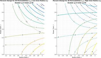
There are now at least two types of linearly graded permeability with an offset that could be compared to the base case. To solve for the necessary offset permeability for this analysis, two types of permeability slope gains, g, were chosen of 5 and 50 and are represented with dashed and solid lines, respectively. The percent change in magnetization losses are shown in Fig. 5 for different geometric and profile design cases. Analytically, the loss ratio is shown in the following equation:
 $${{P\left( {{B_{{\rm{loc ‐ }}{\mu _1}}}} \right)} \over {P\left( {{B_{{\rm{loc ‐ }}{\mu _{\rm{c}}}}}} \right)}} = {\left( {{{ - {r_{\rm{i}}}g\ln \left( \lambda \right)} \over {\ln \left( \lambda \right) + g{r_{\rm{i}}}\left( {\lambda - 1} \right)}}} \right)^\beta }{{\left( {2 - \beta } \right)\left( {{B_{ - g\lambda {r_{\rm{i}}}}}\left[ {2 - \beta ,\;1 + \beta } \right] - {B_{ - g{r_{\rm{i}}}}}\left[ {2 - \beta ,\;1 + \beta } \right]} \right)} \over {{{\left( { - g{r_{\rm{i}}}} \right)}^2}\left( {{\lambda ^{2 - \beta }} - 1} \right)}}\quad .$$
Percent change in magnetization losses for toroids utilizing graded permeability with offset profiles.

From the above figure and (30), there are several interesting conclusions to make. The first being that a low slope gain of permeability can provide some improvements in the magnetic core losses over most of the design space. While these improvements are small, they are nonetheless significant compared to the linear graded permeability with zero offset where all designs had incurred penalty of higher magnetizing losses. Furthermore, the high slope gain also shows some loss improvements. However, these improvements are limited to low inner radius designs with high power terms. For high inner radius designs, the improvements exist in a much smaller design space with penalties that more closely reflect those of the zero offset designs. It is also important to note that all of the trends exist independent of the level of the baseline constant permeability.
Again, the common design of a radius ratio of 2 and loss term of 2.4 is chosen as an example. For low inner radius designs, a low g of 5 results in a negligible loss reduction of 0.2% and for high g of 50, the loss reduction is marginally better at 0.4%. For high inner radius designs, the loss reduction for low gains is still small at 0.4%; however, there is penalty at high gains with a 1.8% loss increase.
E. Exponential permeability
The fourth and final strain annealed permeability profile examined in this analysis is a profile that changes exponentially with the core radius. There is a scalar term defined as µe and the exponent is the variable c. This profile is defined in (31). One motivation of these profiles is to effectively invert the flux density concentration in a core. This would shift the heat injection to the outer edges of the core where the natural thermal impedance to convection and radiation is lower. Similarly, shifting the hotspot to the exterior of a core enables easier access and more surface area for application of cooling through a heat sink or other active measure.
 $$\mu \left( r \right) = {\mu _{\rm{e}}}{r^{\rm{c}}}\quad .$$
The average flux density and core permeance are shown in (32) and (33), respectively.
 $${B_{{\rm{avg ‐ }}{\mu _{\rm{e}}}}} = {{NI} \over {2\pi }}{{{\mu _{\rm{e}}}r_{\rm{i}}^{\rm{c}}\left( {{\lambda ^{\rm{c}}} - 1} \right)} \over {c{r_{\rm{i}}}\left( {\lambda - 1} \right)}}\quad ,$$
 $$\hat{P} = {h \over {2\pi }}{{{\mu _{\rm{e}}}{r_{\rm{i}}}^{\rm{c}}} \over c}\left( {{\lambda ^{\rm{c}}} - 1} \right)\quad .$$
The estimation for power losses using the average flux density is presented in (34). The local heat injection due to localized losses is shown in (35).
 $$P\left( {{B_{{\rm{avg ‐ }}{\mu _{\rm{e}}}}}} \right) = k{f^\alpha }h\pi r_{\rm{i}}^2\left( {{\lambda ^2} - 1} \right){\left( {{{NI} \over {2\pi }}} \right)^\beta }{\left( {{{{\mu _{\rm{e}}}r_{\rm{i}}^{\rm{c}}\left( {{\lambda ^{\rm{c}}} - 1} \right)} \over {c{r_{\rm{i}}}\left( {\lambda - 1} \right)}}} \right)^\beta }\quad ,$$
 $${P_{{\rm{loc ‐ }}{\mu _{\rm{e}}}}} = k{f^\alpha }ht2\pi r{\left( {{{{\mu _{\rm{e}}}{r^{\rm{c}}}NI} \over {2\pi r}}} \right)^\beta }\quad .$$
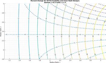
Finally, the losses calculated by using the local flux density are shown in (36). The percent change in losses of the exponential permeability profile is compared to the baseline of constant permeability in Fig. 6 with the corresponding ratio shown in (37).
 $$P\left( {{B_{{\rm{loc ‐ }}{\mu _{\rm{e}}}}}} \right) = k{f^\alpha }h2\pi {\left( {{{NI} \over {2\pi }}} \right)^\beta }{{\mu _{\rm{e}}^\beta {r_{\rm{i}}}^{\beta \left( {c - 1} \right) + 2}\left( {{\lambda ^{\beta \left( {c - 1} \right) + 2}} - 1} \right)} \over {\beta \left( {c - 1} \right) + 2}}\quad ,$$
 $${{P\left( {{B_{{\rm{loc ‐ }}{\mu _{\rm{e}}}}}} \right)} \over {P\left( {{B_{{\rm{loc ‐ }}{\mu _{\rm{c}}}}}} \right)}} = {\left( {{{c\ln \left( \lambda \right)} \over {{\lambda ^{\rm{c}}} - 1}}} \right)^\beta }{{\left( {2 - \beta } \right)\left( {{\lambda ^{\beta \left( {c - 1} \right) + 2}} - 1} \right)} \over {\left( {\beta \left( {c - 1} \right) + 2} \right)\left( {{\lambda ^{2 - \beta }} - 1} \right)}}\quad .$$
Percent change in magnetization losses for toroids utilizing exponential permeability profiles.

The contours of Fig. 6 show the general approach to the exponentially graded permeability profile. The first and foremost observation is that regardless of the inner radius level or the baseline permeability level, the loss changes are the same for this profile when the permeance of the profiles is chosen to match the constant permeability permeance. For this permeability profile type, when the exponent is low, there are some small benefits in overall losses, e.g., a loss reduction of 0.2% for the example core of a radius ratio of 2 with a power term of 2.4. Higher exponents result in higher losses and significantly higher losses as the radius ratio increase with a 9.1% increase in the example core. In fact, with high exponent values, the change in losses depends mostly on the radius ratio.
IV. EXAMPLE COMPARISON OF PERMEABILITY PROFILES
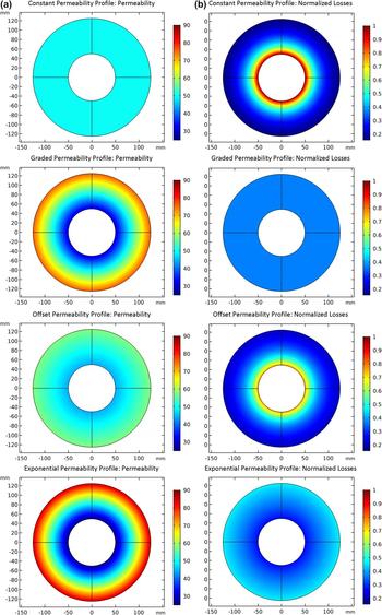
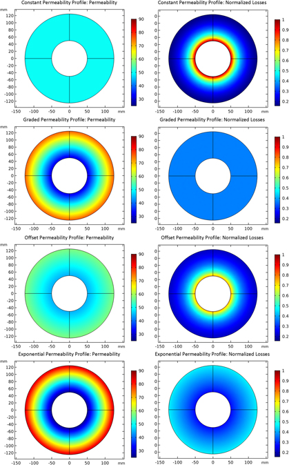
The different strain annealed permeability profiles are compared in an example power inductor through Comsol FEA. This simple design comparison is used to explore the different permeabilities and core loss profiles for practical applications. The permeability profile and loss profile are shown further in Fig. 7. The left column of surface plots shows the relative permeability of the core for the different strain profiles. The right column shows the local loss profile which corresponds to the heat injection, ultimately reflecting core temperature rise due to the thermal anisotropy shown in Fig. 2.
FEA analysis of constant, graded, graded with an offset, exponential (descending) permeability profiles (a) and normalized losses (b) are shown.

For this example, the following variables were set with their corresponding values: with an inner radius, r i = 50 mm, λ = 2.5 for an outer radius, r o = 125 mm, the baseline constant permeability, μc = 50, and the loss term, β = 2.5. To solve for the remaining variables in the offset permeability profile and exponential permeability profile, the values of g and c were set to 5 and 1.3. All free variables are solved to ensure that each strain annealed core has the same inductance as the constant relative permeability design.
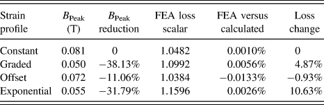
The tabularized results of the flux density, normalized core loss terms, and validity of above presented equations for this example, Table II, show the significance of the controlled strain annealing approach to influence the thermal profile of a magnetic core. For a given inductor, new thermal management regimes can be used. For instance, all strain annealing approaches reduce the peak thermal injection by reducing the local losses in the core. This enables improved performance with minimal redesign. Alternatively, more improvement could be achieved by using either the graded or the exponential approaches in this example that result in the toroid hotspots shifting to the outside. This translates to higher heat injection on the outside of the core from the inside. As discussed above, the outer layers of the core have reduced thermal impedances for heat flow to ambient. Additionally, the outside of the core is usually easier to access physically than the inside of the core. This means that an external heatsink, attached to the outside of the core, can have a greater impact. The heating is now closer to the highest levels of heat injection into the core and thus can better sink heat away from the hotspot of the core.
Tabularized analysis of FEA study of losses and peak flux density for various strain annealing profiles.

These FEA results show that significant improvements in core performance can be achieved through strain annealing. Notably, the peak flux density can be significantly reduced while maintaining the same inductance. The temperature profile can also be tuned and controlled through strain annealing for application advantages. The presented analytical expressions show very close correlation with the FEA analysis and are proven to be valid.
V. HARDWARE EXAMPLE
The controls and processing for managing continuous magnetic ribbon straining have very recently been completed to enable hardware testing. Two cores were manufactured from raw ribbon stock of a cobalt-rich MANC. The as-cast MANC ribbon has a relative permeability around 80. From this stock material, the two cores were subjected to strain annealing to result in a core with a constant relative permeability profile and graded with an offset relative permeability profile.
The constant permeability core was strain annealed to a permeability of μc = 38.3 and confirmed with thin strip testing. The linearly strained permeability is slightly more difficult to determine due to the nonlinear relationship between strain and resulting permeability. However, in this example, the range of strain results in a relatively constant and linear variation. Using strip testing on the beginning and the end of the ribbon, the permeability function was interpolated to be μo(r) = μl + μsr = 17.446 + 334r. The average flux density for the two cores of constant permeability,  ${B_{{\rm{av}}{{\rm{g}}_{{\mu _{\rm{c}}}}}}}$, and graded permeability,
 ${B_{{\rm{av}}{{\rm{g}}_{{\mu _{\rm{o}}}}}}}$, is determined using the Eqs. (10) and (25) from the above analysis. The ratio of power loss is then simply determined by comparing the ratio of power loss using the Steinmetz equation and the respective average flux densities as presented in (30). Due to uncertainties in the final flux density loss term, β, an assumption was made that the two cores had the same β and then the result for a range of values was explored for 2 ≤ β ≤ 2.5. This resulted in a loss ratio of
 $1.185 \le {{P\left( {{\mu _{\rm{c}}}} \right)} \over {P\left( {{\mu _{\rm{o}}}} \right)}} \le 1.376$ for the local flux density method and a loss ratio of
 $1.22 \le {{P\left( {{\mu _{\rm{c}}}} \right)} \over {P\left( {{\mu _{\rm{o}}}} \right)}} \le 1.329$ when the losses are calculated using the average flux density method. These ratios show a predicted reduction in losses by using the strain annealed profile. These analytical predictions match very close to the measured results where the constant permeability core produced 13.11 W of loss and the linearly graded with an offset produced 10.15 W of loss. This resulted in a 22.5% reduction in losses, which agrees very well with the previously stated range of loss reduction.
To complete the comparison, it is important to confirm any variation in the resulting inductance, (38), due exclusively to permeance changes. Ultimately, the graded permeability core will be tuned to perfectly match a homogenous permeability core. However, at this initial stage, small variations in inductance due to high experimental manufacturing tolerances are acceptable. The variation for this experiment is shown below and is shown to be within a low tolerance.
 $${{{L_{{\mu _{\rm{c}}}}}} \over {{L_{{\mu _{\rm{g}}}}}}} = {{{\mu _{\rm{c}}}\ln \left( {{{{r_{\rm{o}}}} \over {{r_{\rm{i}}}}}} \right)} \over {{\mu _{\rm{l}}}\ln \left( {{{{r_{\rm{o}}}} \over {{r_{\rm{i}}}}}} \right) + {\mu _{\rm{s}}}\left( {{r_{\rm{o}}} - {r_{\rm{i}}}} \right)}} = {{38.3\ln \left( {{{0.081} \over {0.031}}} \right)} \over {17.446\ln \left( {{{0.081} \over {0.031}}} \right) + 334\left( {0.081 - 0.031} \right)}} = 1.0995\quad .$$
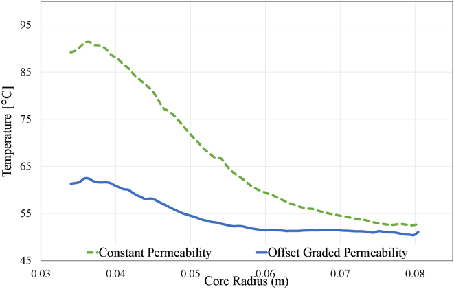
Figure 8 shows a thermal line plot of the temperature of the two cores along the radial dimension. These lines were developed using a FLIR thermal camera and FLIR post-processing software where several temperature measurement lines were taken. Figure 8 shows the average of all of the lines taken at different angles along the radial dimension.Reference Byerly, Ohodnicki, Moon, Leary, Keylin, McHenry, Simizu, Beddingfield, Yu, Feichter, Noebe, Bowman and Bhattacharya36 Further explores the creation, testing, and processing of these cores. While there are obvious visual differences in temperature between the constant permeability core and graded with an offset core, the total reduction in peak temperature is about 30% from nearly 91.6 °C down to about 62.7 °C. Furthermore, the losses measured using the open secondary test, demonstrated in Ref. Reference Thottuvelil, Wilson and Owen37, show a 25% reduction in core magnetization losses. These results correspond to the predicted analytical results and represent a significant improvement core operation. Importantly, this is not a one-to-one comparison of cores as shown in Table II. Manufacturing limitations introduced variations in total inductance while Table II compares designs of the same inductance. However, using the parameters of the constructed inductors to the presented analysis methods correlates very closely with measured results as shown in the analysis above.
Comparison of thermal line plots of steady-state temperature of constant permeability profile (dashed) and offset permeability profile (solid) toroids along radial dimension.

A brief discussion is merited for the relationship between the thermal profiles and loss gradient profiles of Fig. 7. From the loss profiles, one could reasonably expect a constant decay of temperature closely related to the decay of the local losses. However, the temperature near the inner and outer radii is strongly affected by the relatively low total thermal impedance in the radial direction. Specifically, the innermost and outermost layers have a very low impedance to ambient because of their exposed broad surfaces. The two-edge resistive networks in Fig. 2 show this. These relatively cool layers act as sinks to adjacent layers resulting in core temperatures that are lower than one might expect given the heat injection profile. Another aspect of this that is not addressed in Fig. 2 is the heat injection to the core from the exciting coils. This is noticeable by the slight increase in core temperature at the core edges.
VI. IMPLICATIONS AND RECOMMENDATIONS FOR THERMAL MANAGEMENT
As mentioned above, the anisotropic nature of the thermal body enforces the local heating to follow the local loss with minimal transfer across ribbon layers. Because of these phenomena, it is an adequate assumption that the thermal profile and heat injection profile are proportional but follow the same general curve. As such, strain annealing can be used to deliberately assist magnetic core cooling. The following recommendations will provide uses and examples for each of the four presented strain annealed permeability profiles.
The constant permeability profile is the most elementary of the profiles. The manufacturing process is also the simplest as only a single constant tension force is needed. As such, the mechanical limits of the ribbon are less of a concern as the tension can be held within maxima for all designs. Its use and effect has the least variation from a traditional core. However, where the constant permeability core is most applicable in replacing a magnetic component assembled with a core of higher standard relative permeability and an air gap. Now, the gap can be eliminated by using a strain annealed core that has the same effective permeability as the gapped core. This eliminates the additional losses, e.g., fringing and winding proximity, associated with the gap. Thus, a hotspot is eliminated whereby prior cooling is now unnecessary. However, because of the method of tuning for all of the other profiles, this advantage is not unique to this profile.
Linearly graded permeability profiles offer the ability to shift the hottest point of the core to the outer edges. This has the advantage of working better with external heatsinks. This profile has some added complexity in the manufacturing and ribbon stress limits need to be carefully avoided. However, if properly implemented, the core is subjected to a uniform flux density along the radial direction. With increasing volume, this causes a linearly increasing thermal injection to the core. This reduces the thermal gradient to a constant over the entire core profile.
If there are mechanical or magnetic properties that limit full implementation of the linearly graded permeability, adding an offset provides a reliable solution. The resulting thermal profile is similar to the constant permeability case. However, the inner radius peak heat injection is significantly reduced and the outer radius injection is raised slightly. This approach offers one of the most practical design steps as it can accommodate the most constraints and tolerances while still providing the benefit of reduced peak temperatures and potentially reduced losses.
The exponential permeability profile is one of the more interesting cases. While having a minimal dependency on core inner radius and base permeability, this profile can provide three different approaches to heating profiles. Using a low exponent term results in heat injection profiles similar to constant and offset permeabilities. Higher exponents have the ability to shift dramatically the heat injection to the outside of the core. This can result in more efficient external heat sink operation. Finally, by carefully choosing the exponent, the heat injection profile can be reduced to a constant. This uniformly heats the core and eliminates the radially dependent hotspots.
The ability to choose a permeability profile and specific variations in the profile offers a new tool in magnetics design. These variables enable new approaches to multi-objective optimization. New optimization points and designs are available that can fit new operational spaces.
VII. FUTURE WORK AND CONCLUSIONS
Future work will further quantify the magnetic ribbon variations due to strain annealing. This will allow the loss predictions to incorporate these dynamic impacts. Similarly, the loss model will be integrated tightly with the heat injection. This will provide further insight into the optimal strain annealing profiles to achieve final core temperature profiles. Similarly, more experimental results will be developed by assembling cores of the various profiles.
Fundamentally, the process of designing a magnetic core permeability profile using strain annealing offers another tool in a magnetic designer toolbox. Four fundamental profiles were presented with analytical expressions for losses and heat injection. These heat injection terms can be coupled with the presented anisotropic thermal model to better predict a magnetic core thermal profile and to anticipate potential hotspots. This prediction was verified using line scans of two experimental toroid cores employing the constant permeability and linearly graded with offset profiles. Furthermore, the total losses measured were accurately predicted using the presented profile dependent loss equations.
The benefits of the strain annealing tool can come at the cost of increased losses depending on the desired design space. Sets of curves were presented to be used in the design screening process. It was shown that some profiles can reduce the toroid total losses while also providing the aforementioned thermal and flux control benefits. It is with these benefits in mind that new recommendations for a combined design process utilizing strain annealing and heatsink placement was provided for improved cooling performance. Thus, in the process of strain annealing, a magnetic ribbon core to provide a specific permeability profile represents a new paradigm in magnetic core design.
LIST OF SYMBOLS

Supplementary Material
To view supplementary material for this article, please visit https://doi.org/10.1557/jmr.2018.157.
ACKNOWLEDGMENTS
The authors would like to thank the Oak Ridge Institute for Science Education (ORISE) for funding and financial support. Similarly, the authors would like to thank the Department of Energy for support to the diverse team through DOE EERE initiative SuNLaMP program and the National Energy Technology Lab ongoing research under the RES contract DE-FE0004000. The authors also acknowledge funding support through the National Energy Technology Laboratory's research support of the DOE OE Transformer Reliability and Advanced Components (TRAC) Program.