2.1 Dilworth’s theorem

Dilworth’s theorem is a famous combinatorial theorem about partial orders, closely related to bounded Ramsey’s theorem. The width $w(\mathcal {P})$ of a partial order $\mathcal {P} = ({\mathbb {N}}, <_{\mathcal {P}})$ is the size of its largest antichain.

Such a coloring g is called a chain partition of $\mathcal {P}$ . Dilworth’s theorem is classically proven for finite partial orders, but the infinitary version directly follows from it by a compactness argument as follows: Given a partial order $\mathcal {P} = ({\mathbb {N}}, <_{\mathcal {P}})$ of finite width w, one can define its incomparability graph $\mathcal {G} = ({\mathbb {N}}, E)$ , that is, the graph such that $\{x, y\} \in E$ iff x and y are $\mathcal {P}$ -incomparable. Finite Dilworth’s theorem essentially states that the graph $\mathcal {G}$ is locally w-colorable. By Gasarch and Hirst [Reference Gasarch and Hirst16, Theorem 4], ${\mathsf {RCA}}_0 + {\mathsf {WKL}}$ proves that every locally w-colorable graph is w-colorable, and any such w-coloring is a chain partition of G. Thus, Dilworth’s theorem follows from ${\mathsf {RCA}}_0 + {\mathsf {WKL}}$ . Hirst [Reference Hirst19, Theorem 3.23] studied Dilworth’s theorem in reverse mathematics and proved that it is equivalent to ${\mathsf {WKL}}$ over ${\mathsf {RCA}}_0$ , even restricted to partial orders of width 2.

Seeing a partial graph of finite width as a degenerate instance of ${\mathsf {BRT}}^2_2$ , we are interested in the existence of an infinite $\mathcal {P}$ -chain. Given a chain partition $g : {\mathbb {N}} \to k$ , a final application of ${\mathsf {RT}}^1$ suffices to obtain such a chain. Therefore, ${\mathsf {RCA}}_0 + {\mathsf {WKL}} + \mathsf {B}\Sigma ^0_2$ is sufficient to prove that every partial order of finite width admits an infinite chain. Dilworth’s theorem states that the chain partition of $\mathcal {P}$ equals its width, but for our purpose, it is sufficient to consider the following weaker statement.

By Schmerl [Reference Schmerl33], if $2 \leq k \leq m$ , then the statement “Every locally k-colorable graph is m-colorable” is equivalent to ${\mathsf {WKL}}$ over ${\mathsf {RCA}}_0$ . Based on the proof of Dilworth’s theorem, one would naturally expect that weak Dilworth’s theorem remains equivalent to ${\mathsf {WKL}}$ over ${\mathsf {RCA}}_0$ . Surprisingly, Kierstead [Reference Kierstead24] proved that every computable graph with width w admits a computable chain partition of size $(5^w-1)/4$ .

The original proof by Kierstead [Reference Kierstead24] involved strong induction axioms, but in their study of a theorem from Rival and Sands [Reference Rival and Sands32], Fiori-Carones, Marcone, Shafer, Soldà, with the help of Yokoyama, adapted the proof of Kierstead to formalize it over ${\mathsf {RCA}}_0$ (see [Reference Fiori-Carones, Marcone, Shafer and Soldà14, Theorem 3.5]).

Kierstead’s theorem can be stated in the modern formalism as the existence of an on-line algorithm for the chain partition problem, where an on-line algorithm is one that produces its output progressively, as it receives its input, without having access to the entire input in advance. The bound $(5^w-1)/4$ obtained by Kierstead was recently improved by Bosek and Krawczyk [Reference Bosek and Krawczyk5, Reference Bosek and Krawczyk6] to $w^{14\log w}$ and by Bosek et al. [Reference Bartłomiej Bosek, Kierstead, Matecki and Smith2] to $w^{6.5\log w+7}$ . See [Reference Bosek, Felsner, Kloch, Krawczyk, Matecki and Micek4] for a survey on the subject.

The proof of Kierstead’s theorem is complex, but in the case where the partial order is up-growing, there exist significantly simpler algorithms (see Felsner [Reference Felsner12]). A presentation of a partial order is up-growing if each new element is maximal among the elements inputted so far. The following proposition is essentially a reformulation of Felsner’s algorithm [Reference Felsner12] in our formalism, in which an up-growing partial order can be seen as a coloring $f : [{\mathbb {N}}]^2 \to 2$ which is transitive for color 0. Indeed, any such coloring can be seen as the partial order $\mathcal {P} = ({\mathbb {N}}, <_{\mathcal {P}})$ defined by $x <_{\mathcal {P}} y$ iff $x <_{\mathbb {N}} y$ and $f(x, y) = 0$ .

This simpler algorithm is sufficient to obtain another proof that ${\mathsf {EM}}$ implies ${\mathsf {BRT}}^2_2$ over ${\mathsf {RCA}}_0$ .

2.2 Mirsky’s theorem

Dilworth’s theorem admits a dual version for partial orders with chains of bounded size, due to Mirsky [Reference Mirsky29]. The height $h(\mathcal {P})$ of a partial order $\mathcal {P} = ({\mathbb {N}}, <_{\mathcal {P}})$ is the size of its largest $\mathcal {P}$ -chain.

Accordingly, such a coloring g is called an antichain partition of $\mathcal {P}$ . Contrary to Dilworth’s theorem, Mirsky’s theorem admits a trivial combinatorial proof: Given a partial order $\mathcal {P} = ({\mathbb {N}}, <_{\mathcal {P}})$ of finite height h, define $g : {\mathbb {N}} \to h$ as follows: $g(x)$ is the size of the largest $\mathcal {P}$ -chain with x as $\mathcal {P}$ -maximal element. However, from a reverse mathematical viewpoint, the definition of g requires an unbounded search for such a $\mathcal {P}$ -chain, and is formalized over ${\mathsf {ACA}}_0$ . Hirst [Reference Hirst19] actually showed that Mirsky’s theorem is equivalent to ${\mathsf {WKL}}$ (and therefore to Dilworth’s theorem) over ${\mathsf {RCA}}_0$ , even when restricted to partial orders of height 2.

The proof of Mirsky’s theorem over ${\mathsf {RCA}}_0 + {\mathsf {WKL}}$ is very similar to that if Dilworth’s theorem, this time using the comparability graph. As for Dilworth’s theorem, one can define a weak version of the statement.

The natural combinatorial proof of Mirsky’s theorem can be refined, to yield a proof of weak Mirsky’s theorem over ${\mathsf {RCA}}_0$ .

Mimouni and Patey [Reference Mimouni and Patey28] defined an asymmetric version of the ${\mathsf {EM}}$ in which the solution is required to be transitive for one color at least.

By combining Propositions 2.5 and 2.8, one obtains the following implication. It is unknown whether ${\mathsf {HEM}}$ implies $\mathsf {B}\Sigma ^0_2$ over ${\mathsf {RCA}}_0$ .

3.1 Models of weak arithmetic and cuts

A structure in the language of second-order arithmetic is a tuple

$$ \begin{align*}\mathcal{M} = (M, S, 0, 1, +, \times, <), \end{align*} $$

where M denotes the set of integers, $S \subseteq \mathcal {P}(M)$ is the collection of sets of integers, $0$ and $1$ are constants in M, $+, \times : M^2 \to M$ are binary operations, and $<$ is a binary relation on M. We shall exclusively work with structures which are models of ${\mathsf {RCA}}_0$ , and simply call them models, and usually abbreviate them by $\mathcal {M} = (M, S)$ . A model $\mathcal {M} = (M, S)$ is topped by a set $Y \in S$ if every set in S is $\Delta _1(Y)$ -definable with parameters in M.

A model where M is the set of standard integers $\omega = \{0, 1, \dots \}$ will be called an $\omega $ -model, if $M \neq \omega $ , then the model is said to be non-standard.

In a non-standard model, the elements $0, 1, 1 + 1, 1 + 1 + 1, \dots $ form a cut which can be identified with $\omega $ . The amount of induction satisfied by a model corresponds to the difficulty of having cuts that are definable.

Finite/infinite sets. In models of weak arithmetic, the various definitions of infinity are not necessarily equivalent, and require a precise terminology. A subset $X \subseteq M$ is said to be M-bounded if there exists some $y \in M$ such that $x < y$ for every $x \in X$ . If no such y exists, X is said to be M-unbounded. In a model $\mathcal {M} = (M, S) \models {\mathsf {RCA}}_0$ , the M-bounded sets belonging to S will be called $\mathcal {M}$ -finite and the M-unbounded $\mathcal {M}$ -infinite.

Every element $a \in M$ can be seen as the binary encoding of some M-bounded set $F \subseteq M$ and we write $a = \sum _{x \in F} 2^x$ . Not all M-bounded sets can be M-coded by some integer $a \in M$ , but if $\mathcal {M} = (M, S) \models {\mathsf {RCA}}_0$ , then the M-coded sets are exactly the $\mathcal {M}$ -finite, hence, the $\mathcal {M}$ -finite sets only depend on the first order part M of the model $\mathcal {M}$ and we will call them M-finite to emphasize on that.

Cofinal functions. The lack of induction can also be measured in the existence of definable cofinal functions from a proper cut to M. This will be of central importance for proving Main Theorem 1.4. For $I \subseteq M$ a cut, a function $g : I \to M$ is said to be cofinal (in M) if its range is M-unbounded.

In particular, if $\mathcal {M} = (M, S) \models {\mathsf {RCA}}_0 + \mathsf {B}\Sigma ^0_2 + \neg \mathsf {I}\Sigma ^0_2$ and $I \subseteq M$ is a $\Sigma ^0_2$ -cut bounded by some $k \in M$ , one can assume that the function g can be approximated by a $\Delta ^0_1$ sequence of functions $(g_s)_{s \in M}$ such that for every $s \in M$ , $g_s : k \to M$ is increasing, and for every $x < k$ , $s \mapsto g_s(x)$ is non-decreasing, dominated by $s \mapsto s$ , and converges to $g(x)$ . One can also assume that for every $s \in M$ and $x < k$ , if $g_{s+1}(x) \neq g_s(x)$ then $g_{s+1}(s) = s+1$ . Hence, if $g(x) = s$ for some $x \in I$ and $s \in M$ , then $g_s(x) = g(x)$ .

3.2 Main result

In what follows, a $\Sigma _n(X)$ -formula (resp. a $\Pi _n(X)$ -formula or $\Delta _n(X)$ -formula) is a $\Sigma _n^0$ -formula (resp. a $\Pi _n^0$ -formula or $\Delta _n^0$ -formula) with only X as a second-order parameter and any first-order parameters.

The core of the argument lies in the following technical lemma.

We are now ready to prove our first main theorem.

Note that the previous argument is very general: if $\mathsf {I}\Sigma ^0_2$ implies a $\Pi ^1_2$ -problem $\mathsf {P}$ over ${\mathsf {RCA}}_0$ , then ${\mathsf {RCA}}_0 + \mathsf {I}\Sigma ^0_2 \vdash $ “ $\mathsf {P}$ is computably true.” One could also have simply noticed that the proof of Proposition 2.1 yields a computable solution.

4.1 Strategy to prove Main Theorem 1.5

Before going into the technicalities, let us first outline the proof of Main Theorem 1.5. It is divided into the following steps:

Step 1. Consider any countable model $\mathcal {M}_0 = (M, S_0)$ of ${\mathsf {RCA}}_0 + \mathsf {B}\Sigma ^0_2 + \neg \mathsf {I}\Sigma ^0_2$ topped by some set $Z_0$ . By Main Theorem 1.4, $\mathcal {M}_0$ contains a stable instance f of ${\mathsf {BRT}}^2_2$ with no $\Delta _1(Z_0)$ -definable solution. Let $A = \{ x \in M : \forall ^\infty y f(x, y) = 0 \}$ . The set A is $\Delta _2\text {-}\mathsf {Def}(\mathcal {M}_0)$ and $Z_0$ -immune. Actually, the proof of Main Theorem 1.4 shows that A satisfies a stronger notion of immunity, that we call for now sufficient $Z_0$ -immunity.

Step 2. Given a countable model $\mathcal {M}_n = (M, S_n)$ of ${\mathsf {RCA}}_0 + \mathsf {B}\Sigma ^0_2$ topped by a set $Z_n$ , and any sufficiently $Z_n$ -immune set $A \subseteq M$ , we shall prove that for every instance $\mathcal {L}$ of ${\mathsf {SADS}}$ in $\mathcal {M}_n$ , there is a solution G such that A is sufficiently $G \oplus Z_n$ -immune, and $\mathcal {M}_n[G] \models {\mathsf {RCA}}_0 + \mathsf {B}\Sigma ^0_2$ . Then, let $\mathcal {M}_{n+1} = \mathcal {M}_n[G]$ be the $\omega $ -extension of $\mathcal {M}_n$ topped by $Z_{n+1} = G \oplus Z_n$ (Proposition 4.4).

Step 3. Given a countable model $\mathcal {M}_n = (M, S_n)$ of ${\mathsf {RCA}}_0 + \mathsf {B}\Sigma ^0_2$ topped by a set $Z_n$ , and any sufficiently $Z_n$ -immune set $A \subseteq M$ , we shall prove that for every instance $\vec {R}$ of ${\mathsf {COH}}$ in $\mathcal {M}_n$ , there is a solution G such that A is sufficiently $G \oplus Z_n$ -immune, and $\mathcal {M}_n[G] \models {\mathsf {RCA}}_0 + \mathsf {B}\Sigma ^0_2$ . Then, let $\mathcal {M}_{n+1} = \mathcal {M}_n[G]$ be the $\omega $ -extension of $\mathcal {M}_n$ topped by $Z_{n+1} = G \oplus Z_n$ (Proposition 4.17).

Step 4. Apply iteratively Steps 2 and 3 to obtain an infinite sequence of countable models $\mathcal {M}_0, \mathcal {M}_1, \dots $ of ${\mathsf {RCA}}_0 + \mathsf {B}\Sigma ^0_2$ such that for each $n \in \omega $ , $\mathcal {M}_{n+1}$ is topped by $Z_n$ , $\omega $ -extends $\mathcal {M}_n$ , and A is sufficiently $Z_n$ -immune, where A is the $\Delta _2(\mathcal {M}_0)$ set defined in Step 1. A union of models of ${\mathsf {RCA}}_0 + \mathsf {B}\Sigma ^0_2$ is again a model of ${\mathsf {RCA}}_0 + \mathsf {B}\Sigma ^0_2$ , and if the instances of ${\mathsf {SADS}}$ and ${\mathsf {COH}}$ are properly listed, then $\mathcal {N} = \bigcup _n \mathcal {M}_n$ is a model of ${\mathsf {SADS}} + {\mathsf {COH}}$ , hence of ${\mathsf {ADS}}$ . Moreover, A is sufficiently immune relative to every set in $\mathcal {N}$ , so the instance of ${\mathsf {BRT}}^2_2$ defined in Step 1 has no solution in $\mathcal {N}$ , hence $\mathcal {N} \not \models {\mathsf {BRT}}^2_2$ .

4.2 Combinatorics of ${\mathsf {ADS}}$

In order to get a better grasp of the appropriate notion of immunity to consider, let us dig into the combinatorics of ${\mathsf {ADS}}$ . There exists mainly two forcing constructions to build solutions to ${\mathsf {ADS}}$ . The first one is asymmetric, and was used by Hirschfeldt and Shore [Reference Hirschfeldt and Shore18, Proposition 2.26] to prove that ${\mathsf {ADS}}$ does not imply the existence of DNC functions over ${\mathsf {RCA}}_0$ . A function $g : {\mathbb {N}} \to {\mathbb {N}}$ is diagonally non-X-computable (X-DNC) if for every $e \in {\mathbb {N}}$ , $g(e) \neq \Phi ^X_e(e)$ . The second forcing construction is symmetric, and was defined by Lerman et al. [Reference Lerman, Solomon and Towsner26] and later used by Patey [Reference Patey31] to give an alternative proof of [Reference Hirschfeldt and Shore18, Proposition 2.26].

The combinatorics of ${\mathsf {ADS}}$ are already witnessed by stable linear orders, so let us fix a computable stable linear order $\mathcal {L}= ({\mathbb {N}}, <_{\mathbb {N}})$ . If it is of order type $\omega +k$ or $k+\omega ^*$ , then there is an infinite computable $\mathcal {L}$ -ascending or $\mathcal {L}$ -descending sequence, so let us assume that it is of order type $\omega +\omega ^*$ . Let $U^0$ and $U^1$ be its sets of $\mathcal {L}$ -small and $\mathcal {L}$ -large elements, respectively. Note that $U^0 \sqcup U^1 = {\mathbb {N}}$ and both sets are $\Delta ^0_2$ .

The natural notion of forcing for building solutions to $\mathcal {L}$ is of disjunctive nature. A condition is a pair $(\sigma ^0, \sigma ^1)$ such that $\sigma ^0$ and $\sigma ^1$ are finite $\mathcal {L}$ -ascending and $\mathcal {L}$ -descending sequences, respectively. To ensure the extensibility of each initial segment, one furthermore requires that $\sigma ^0 \subseteq U^0$ and $\sigma ^1 \subseteq U^1$ . Because of this restriction, being a condition is a $\Delta ^0_2$ predicate. A condition $(\tau ^0, \tau ^1)$ extends $(\sigma ^0, \sigma ^1)$ if $\sigma ^i \preceq \tau ^i$ for both $i < 2$ .

Thankfully, one can define a computable notion of split pair, which is a pair $(\sigma ^0, \sigma ^1)$ such that $\sigma ^0$ is $\mathcal {L}$ -ascending, $\sigma ^1$ is $\mathcal {L}$ -descending, and $\max _{\mathcal {L}} \sigma ^0 <_{\mathcal {L}} \min _{\mathcal {L}} \sigma ^1$ . The core of the combinatorics of ${\mathsf {ADS}}$ lies in the following fact.

Let us explain how the combinatorics above enable to have a short c.e. description of large subsets of G-c.e. sets, where G is the constructed solution. Fix a condition $p = (\sigma ^0, \sigma ^1)$ and two Turing indices $e_0, e_1 \in {\mathbb {N}}$ . Let $a_0, a_1 : {\mathbb {N}} \to {\mathbb {N}}$ be defined as follows: for every $t \in {\mathbb {N}}$ , $W_{a_0(t)}$ and $W_{a_1(t)}$ search for a split pair $(\tau ^0, \tau ^1)$ below p such that $\operatorname {card} W^{\tau ^0}_{e_0} \geq t$ and $\operatorname {card} W^{\tau ^1}_{e_1} \geq t$ . If such a split pair exists, then $W_{a_0(t)} = W^{\tau ^0}_{e_0}$ and $W_{a_1(t)} = W^{\tau ^1}_{e_1}$ . By the combinatorics above, for every t, if such a pair exists, then there is an extension q of p forcing either $W_{a_0(t)} \subseteq W^{G^0}_{e_0}$ or $W_{a_1(t)} \subseteq W^{G^1}_{e_1}$ . Otherwise, there is an extension q of p forcing either $\operatorname {card} W^{G^0}_{e_0} < t$ or $\operatorname {card} W^{G^1}_{e_1} < t$ . Last, note that p, $e_0$ , and $e_1$ being fixed, the functions $a_0$ and $a_1$ have a growth in $\mathcal {O}(t)$ for an appropriate numbering.

Such combinatorics are particularly useful when dealing with preservation of effective notions of immunity.

We simply say that A is effectively Z-immune if it is h-effectively immune for a Z-computable function h. Arslanov et al. [Reference Arslanov, Nadirov and Solov’ev1] proved that every effectively immune set computes a DNC function, and conversely, Jockusch [Reference Jockusch23] proved that every DNC function computes an effectively immune set, witnessed by the identity function. Let A be such an effectively immune set. By slightly modifying the above argument, using Kleene’s fixpoint theorem, one can easily obtain indices $a_0$ and $a_1$ such that $W_{a_0}$ and $W_{a_1}$ search for a split pair $(\tau ^0, \tau ^1)$ below p such that $\operatorname {card} W^{\tau ^0}_{e_0} \geq a_0$ and $\operatorname {card} W^{\tau ^1}_{e_1} \geq a_1$ . Then, if such a split pair exists, there is an extension q forcing $W_{a_0} \subseteq W^{G^0}_{e_0}$ or $W_{a_1} \subseteq W^{G^1}_{e_1}$ , hence forcing $W^{G^0}_{e_0} \not \subseteq A$ or $W^{G^1}_{e_1} \not \subseteq A$ .

In our setting, the appropriate notion of immunity will be the following variant of effective immunity. Let $(n, a) \mapsto 2_n(a)$ be the tetration function defined inductively as follows: $2_0(a) = a$ and $2_{n+1}(a) = 2^{2_n(a)}$ .

4.3 Effective constructions over $\mathsf {B}\Sigma ^0_2 + \neg \mathsf {I}\Sigma ^0_2$

The proofs of Propositions 4.4 and 4.17 are done by effectivizations of forcing constructions over non-standard models. By an isomorphism theorem of Fiori-Carones et al. [Reference Fiori-Carones, Kołodziejczyk, Wong and Yokoyama13], there are some deep reasons why, given a $\Pi ^1_2$ -problem $\mathsf {P}$ , any $\omega $ -extension of a model of ${\mathsf {RCA}}_0 + \mathsf {B}\Sigma ^0_2 + \neg \mathsf {I}\Sigma ^0_2$ into a model of ${\mathsf {RCA}}_0 + \mathsf {B}\Sigma ^0_2 + \mathsf {P}$ should be through a first-jump control construction effective in any PA degree over $\emptyset '$ . This will be in particular the case in our construction.

Effective constructions in models of arithmetic with restricted induction raise some new issues. Indeed, given a countable model $\mathcal {M} = (M, S)$ , suppose one builds a set $G \subseteq M$ satisfying a countable sequence of requirements $(\mathcal {R}_e)_{e \in M}$ using an effectivized forcing argument. Let $(\mathbb {P}, \leq )$ be the associated notion of forcing. In order to effectivize the argument, each condition $p \in \mathbb {P}$ is given a code $\langle p \rangle \in {\mathbb {N}}$ and the decreasing sequence of conditions must be represented by a $\emptyset '$ -effective decreasing sequence of codes.

In the standard setting, that is, $M = \omega $ , one can consider each requirement $\mathcal {R}_e$ individually, prove a density lemma saying that every condition p has an extension q forcing $\mathcal {R}_e$ , and then build an infinite descending sequence of conditions $p_0 \geq p_1 \geq \dots $ such that $p_{n+1}$ forces $\mathcal {R}_n$ . On the other hand, if $\mathcal {M} \models \mathsf {B}\Sigma ^0_2 + \neg \mathsf {I}\Sigma ^0_2$ , it might be the case that the decreasing sequence is defined only on a proper $\Sigma ^0_2$ -cut $I \subseteq M$ , that is, only $(p_i)_{i \in I}$ is defined and only the requirements $(\mathcal {R}_i)_{i \in I}$ are satisfied. Note that in this case, the sequence of codes $(\langle p_i\rangle )_{i \in I}$ is unbounded in M, otherwise the cut I would admit a $\Delta ^0_2$ -description, contradicting the fact that $\mathcal {M} \models \mathsf {B}\Sigma ^0_2$ .

To overcome this issue, instead of proving a density lemma for each requirement $\mathcal {R}_e$ individually, we will prove a stronger lemma, stating that for every $k \in M$ and every condition p, there is an extension q forcing $\mathcal {R}_e$ for every $e < k$ simultaneously. Then, using this density lemma, build a decreasing sequence of conditions $p_0 \geq p_1 \geq \dots $ such that $p_{i+1}$ forces $\mathcal {R}_e$ for every $e < \langle p_i\rangle $ simultaneously. Even if the sequence is only defined on a proper cut I, all the requirements $(\mathcal {R}_e)_{e \in M}$ will be forced. This technique is known as Shore blocking.

4.4 The ${\mathsf {SADS}}$ step

We now prove the existence of $\omega $ -extensions which add solutions to instances of ${\mathsf {SADS}}$ while preserving the fact that the instance of ${\mathsf {BRT}}^2_2$ has no solution.

Proof. The following proof is adapted from [Reference Le Houérou, Patey and Yokoyama20, Proposition 3.17].

Let $\mathcal {L} = (M, \leq _{\mathcal {L}})$ be an instance of ${\mathsf {SADS}}$ in S, and let $U^0 \subseteq M$ and $U^1 \subseteq M$ be the sets of elements that have a finite amount of predecessors and successors, respectively. By assumption, $U^0 \sqcup U^1 = M$ , and $U^0$ and $U^1$ are both $\Delta _2(Y)$ . If either $U^0$ or $U^1$ is M-bounded, then there exists some $\mathcal {M}$ -infinite Y-computable $\mathcal {L}$ -monotonous sequence and we can take G to be such a sequence, hence, from now on, both $U^0$ or $U^1$ will be assumed to be M-unbounded.

For simplicity of notation, the elements $b \in B$ will all be assumed to be of the form $2^{2^k}$ for some $k \in M$ , which will then be used to construct $\hat {B}$ such that $\hat {B} \subseteq \{\log _2(\log _2(b)) : b \in B\}$ . The general case requires some care in handling integer parts and inequalities, but does not change the argument.

We will define two sets $G^0$ or $G^1$ using an infinite $\Delta _1(Y')$ decreasing sequence of conditions and then pick G to be equal to one of them. We will also define two $\Delta _1(Y')$ sets $B^i$ for $i < 2$ so that, if $G = G^i$ , then A is $B^i$ -block $(G \oplus Y)$ -immune with cost $n+2$ .

Definition 4.5. A condition is a pair $(\sigma ^0, \sigma ^1)$ with $\sigma ^0$ an M-finite $\mathcal {L}$ -ascending sequence included in $U^0$ and $\sigma ^1$ an M-finite $\mathcal {L}$ -descending sequence included in $U^1$ . We have $(\tau ^0, \tau ^1) \leq (\sigma ^0, \sigma ^1)$ if $\tau ^0 \succeq \sigma ^0$ and $\tau ^1 \succeq \sigma ^1$ .

Being a condition is a $\Delta _2(Y)$ -predicate, while the extension relation is $\Delta _1$ . We define a weaker notion of pair which is $\Delta _1(Y)$ .

Definition 4.6. A split pair is a pair $(\sigma ^0, \sigma ^1)$ of strings such that $\sigma ^0$ is an M-finite $\mathcal {L}$ -ascending sequence, $\sigma ^1$ is an M-finite $\mathcal {L}$ -descending sequence, and $\max _{\mathcal {L}} \sigma ^0 <_{\mathcal {L}} \min _{\mathcal {L}} \sigma ^1$ .

As mentioned in Section 4.2, the core property of split pairs $(\sigma ^0, \sigma ^1)$ comes from the fact that if $\sigma ^i \not \subseteq U^i$ for some $i < 2$ , then $\sigma ^{1-i} \subseteq U^{1-i}$ . In particular, if $(\sigma ^0, \sigma ^1)$ is a condition and $(\tau ^0, \tau ^1)$ is a split pair such that $\sigma ^0 \preceq \tau ^0$ and $\sigma ^1 \preceq \tau ^1$ , then either $(\tau ^0, \sigma ^1)$ or $(\sigma ^0, \tau ^1)$ is a valid condition extending $(\sigma ^0, \sigma ^1)$ . Given two split pairs $(\sigma ^0, \sigma ^1)$ and $(\tau ^0, \tau ^1)$ , we write $(\tau ^0, \tau ^1) \leq (\sigma ^0, \sigma ^1)$ if $\sigma ^i \preceq \tau ^i$ for each $i < 2$ .

Definition 4.7. Let $(\sigma ^0, \sigma ^1)$ be a condition, $e, x \in M,$ and $i < 2$ , we write:

• • $(\sigma ^0, \sigma ^1) \Vdash _i \Phi _e^{G^i \oplus Y}(x) \downarrow $ if $\Phi _e^{\sigma ^i \oplus Y}(x) \downarrow $ .

• • $(\sigma ^0, \sigma ^1) \Vdash _i \Phi _e^{G^i \oplus Y}(x) \uparrow $ if for every split pair $(\tau ^0, \tau ^1) \leq (\sigma ^0, \sigma ^1)$ with $\tau ^{1-i} = \sigma ^{1-i}$ , we have $\Phi _e^{\tau ^i \oplus Y}(x)\uparrow $ .

The relation $(\sigma ^0, \sigma ^1) \Vdash _i \Phi _e^{G^i \oplus Y}(x) \downarrow $ is $\Delta _1(Y)$ and the relation $(\sigma ^0, \sigma ^1) \Vdash _i \Phi _e^{G^i \oplus Y}(x) \uparrow $ is $\Pi _1(Y)$ , both uniformly in their parameters. The formulas $\Phi _e^{G^i \oplus Y}(x) \downarrow $ and $\Phi _e^{G^i \oplus Y}(x) \uparrow $ are universally $\Sigma _1(G^i \oplus Y)$ and $\Pi _1(G^i \oplus Y),$ respectively, and the above definition induces a forcing relation on these classes of formulas.

We want our construction to force for some $i < 2$ the following requirements for every $k \in M$ :

• • $\mathcal {R}^i_k$ : $(G^i \oplus Y)' \upharpoonright _k$ is decided, that is, there exists some $\sigma ' \in 2^k$ such that $(G^i \oplus Y)' \upharpoonright _k = \sigma '$ .

• • $\mathcal {S}^i_{k}$ : There exists some $\ell> 2^{2^k}$ in B, such that, for every $x < \log _2(\log _2(\ell ))$ , if $\operatorname {card} W^{G^i \oplus Y}_x \geq 2_n(\ell )$ , then, there exists some $e < \ell $ such that $\operatorname {card} W_e^Y \geq 2_n(\ell )$ and $W_e^Y \subseteq W_x^{G^i \oplus Y}$ (in particular, since A is B-block Y-immune with cost n, this implies that $W_e^Y \not \subseteq A$ , hence that $W^{G^i \oplus Y}_x \not \subseteq A$ ).

• • $\mathcal {T}^i_k$ : $\exists x> k, x \in G^i$ .

For this, we will use a pairing argument, and ensure that for every $k \in M$ , the following requirements are forced: $\mathcal {R}^0_k \vee \mathcal {R}^1_k$ , $\mathcal {R}^0_k \vee \S ^1_k$ , $\S ^0_k \vee \mathcal {R}^1_k$ , $\S ^0_k \vee \S ^1_k$ , and $\mathcal {T}^0_k \wedge \mathcal {T}^1_k$ .

In what follows, $(\sigma ^0, \sigma ^1) \Vdash _i \mathcal {R}_k^i$ means that there exists some $\sigma ' \in 2^k$ such that $(\sigma ^0, \sigma ^1) \Vdash _i \Phi _e^{G^i \oplus Y}(e) \downarrow $ for every $e < k$ such that $\sigma '(e) = 1$ and $(\sigma ^0, \sigma ^1) \Vdash _i \Phi _e^{G^i \oplus Y}(e) \uparrow $ for every $e < k$ such that $\sigma '(e) = 0$ . Similarly $(\sigma ^0, \sigma ^1) \Vdash _i \S _k^i$ means that there exists some $\ell> 2^{2^k}$ in B such that for every $x < \log _2(\log _2(\ell ))$ , either $(\sigma ^0, \sigma ^1)$ forces $\operatorname {card} W_x^{G^i \oplus Y} < 2_n(\ell )$ or forces $\operatorname {card} W_x^{G^i \oplus Y} \geq 2_n(\ell )$ , and in that case $(\sigma ^0, \sigma ^1)$ also forces $W_e^Y \subseteq W_x^{G^i \oplus Y}$ for some $e < \ell $ such that $\operatorname {card} W_e^Y \geq 2_n(\ell )$ . The requirement $\mathcal {T}^1_k$ is already a $\Sigma _1(G)$ formula, and the forcing relation has already been defined for such formulas.

Definition 4.8. Fix a condition $(\sigma ^0, \sigma ^1)$ . A $(\sigma ^0, \sigma ^1)$ -tree is a binary tree $T \subseteq 2^{<M}$ labelled by a family of split pairs $(\sigma ^0_{\rho }, \sigma ^1_{\rho })_{\rho \in T}$ such that for all $\rho \in T$ :

• • $\sigma ^0 \preceq \sigma ^0_{\rho }$ and $\sigma ^1 \preceq \sigma ^1_{\rho }$ ;

• • for every $\mu \in T$ and every $i < 2$ , if $\rho \cdot i \preceq \mu $ then $\sigma ^i_{\rho } \preceq \sigma ^i_{\mu }$ .

A node $\rho $ is said to be valid if for every $i < 2$ and every $\mu \in T$ such that $\mu \cdot i \preceq \rho $ , then $\sigma ^i_\mu \subseteq U^i$ . Being valid is a $\Delta _2(Y)$ condition.

Definition 4.9. Let T be a $(\sigma ^0,\sigma ^1)$ -tree.

• • A node $(\sigma ^0_{\rho }, \sigma ^1_{\rho })$ in T satisfies a pair of $\Sigma _1(Y)$ -formulas $(\varphi _0(G^0, x), \varphi _1(G^1,x))$ if $\varphi _0(\sigma ^0_{\rho }, |\rho | - \operatorname {card} \rho )$ and $\varphi _1(\sigma ^1_{\rho }, \operatorname {card} \rho )$ hold (where $\operatorname {card} \rho $ is the cardinal of $\rho $ seen as a set, to be distinguished from the length $|\rho |$ of $\rho $ as a string).

• • T satisfies $(\varphi _0(G^0, x), \varphi _1(G^1,x))$ if every node of T satisfies it.

Lemma 4.10. For every pair $(\varphi _0(G^0, x), \varphi _1(G^1,x))$ of $\Sigma _1(Y)$ formulas and every condition $(\sigma ^0, \sigma ^1)$ , there is a maximal $\Sigma _1(Y) (\sigma ^0, \sigma ^1)$ -tree T satisfying it.

Proof. Same as [Reference Le Houérou, Patey and Yokoyama20, Lemma 3.22].

The tree T obtained in [Reference Le Houérou, Patey and Yokoyama20, Lemma 3.22] is given by the limit of a uniformly Y-computable increasing sequence $(T_s)_{s \in M}$ of M-finite $(\sigma ^0, \sigma ^1)$ -trees. This sequence can be uniformly Y-computed in the pair $(\varphi _0(G^0, x), \varphi _1(G^1,x))$ and in the condition $(\sigma ^0, \sigma ^1)$ . Thus, there exists some computable function $e : M \to M$ such that $W^Y_{e(\langle \ulcorner \varphi _0\urcorner , \ulcorner \varphi _1\urcorner , \sigma ^0, \sigma ^1, \rho ,i,x\rangle )}$ searches the split pair $(\sigma ^0_{\rho }, \sigma ^1_{\rho })$ in position $\rho $ of the corresponding $(\sigma ^0, \sigma ^1)$ -tree T, and, if such a split pair exists, outputs the elements of $W_{x}^{\sigma ^i_{\rho } \oplus Y}$ .

Lemma 4.11. Let $(\sigma ^0, \sigma ^1)$ be a condition, $(\varphi _0(G^0, x), \varphi _1(G^1,x))$ be a pair of $\Sigma _1(Y)$ formulas, and T be an M-finite maximal $(\sigma ^0, \sigma ^1)$ -tree satisfying $(\varphi _0(G^0, x), \varphi _1(G^1,x))$ . Then there is some $i < 2$ , some extension $(\hat \sigma ^0, \hat \sigma ^1) \leq (\sigma ^0, \sigma ^1)$ , some $p_i\in M \cup \{-1\}$ such that the following holds:

• • $(\hat \sigma ^0, \hat \sigma ^1) \Vdash _i \varphi _i(G^i, p_i).$

• • $(\hat \sigma ^0, \hat \sigma ^1) \Vdash _i \neg \varphi _i(G^i,p_i+1)$ .

With the convention that $(\hat \sigma ^0, \hat \sigma ^1) \Vdash _i \varphi _i(G^i,-1)$ always holds.

The side $i < 2$ and the extension $(\hat \sigma ^0, \hat \sigma ^1)$ are $Y'$ -computable from $(\sigma ^0, \sigma ^1)$ . Furthermore, $\hat \sigma ^i$ is an element of some split pair appearing in T, i.e., there exists some $\rho \in T$ such that $\hat \sigma ^i = \sigma ^i_{\rho }$ .

Proof. Same as Lemma 3.23 in the arXiv versionFootnote ² of [Reference Le Houérou, Patey and Yokoyama20].

Lemma 4.12. Let $k \in M$ and $(\sigma ^0, \sigma ^1)$ be a condition. Then, for every requirements $\mathcal {U}^0_k \in \{\mathcal {R}^0_k, \S ^0_k\}$ and $\mathcal {U}^1_k \in \{\mathcal {R}^1_k, \S ^1_k\}$ 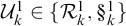, there exists some extension $(\hat \sigma ^0, \hat \sigma ^1) \leq (\sigma ^0, \sigma ^1)$ and some $i < 2$ such that $(\hat \sigma ^0, \hat \sigma ^1) \Vdash _i \mathcal {U}^i_k$ . Such an extension is uniformly $Y'$ -computable in $\mathcal {U}_k^0, \mathcal {U}_k^1$ and $(\sigma ^0, \sigma ^1)$ .

Proof. We will define two $\Sigma _1(Y)$ -formulas $\Phi _t(G,x)$ and $\Psi _t(G,x)$ as follows.

Let $\Phi _{t}(G,x)$ be the formula: $\exists e_0 < e_1 < \dots < e_{x} < t$ such that $\Phi _{e_i}^{G \oplus Y}(e_i) \downarrow $ for every $i \leq x$ , and let $\Psi _t(G,x)$ be the formula: $\exists e_0 < e_1 < \dots < e_{x} < t$ such that $\operatorname {card} W_{e_i}^{G \oplus Y} \geq 2_{n+2}(t)$ for every $i \leq x$ .

Consider the function $S : M \to M$ which maps t to the biggest value taken by $e(\ulcorner \varphi _0 \urcorner , \ulcorner \varphi _1 \urcorner , \sigma ^0, \sigma ^1, \rho , i, x)$ for every $\varphi _0, \varphi _1 \in \{\Phi _t, \Psi _t \}$ , every $\rho \in 2^{\leq 2(t-1)}$ , every $i < 2,$ and every $x < t$ .

Assuming a reasonable encoding of e and of $\Phi _t$ and $\Psi _t$ , this function grows slower than $t \mapsto 2^{2^t}$ , indeed, all the possible parameters of e either directly depend on t (such as $\ulcorner \varphi _0 \urcorner $ and $\ulcorner \varphi _1 \urcorner $ ), are smaller than t (such as x), or are in $2^{\leq 2(t-1)}$ (like $\rho $ ), hence, in any case they can be encoded using $\alpha t$ bits for some $\alpha \in \omega $ and the same holds for the corresponding value taken by e. Hence, there exists some element $\ell $ in B such that $\ell>2^{2^{k}}$ and such that $\ell ' := \log _2(\log _2(\ell ))$ satisfies $S(\ell ') < 2^{2^{\ell '}} = \ell $ .

For every $i < 2$ , let $\varphi _i(G,x)$ be the formula $\Phi _{\ell '}(G,x)$ if $\mathcal {U}^i_k = \mathcal {R}^i_k$ and $\Psi _{\ell '}(G,x)$ otherwise.

Let T be the maximal $\Sigma _1(Y) (\sigma ^0, \sigma ^1)$ -tree T satisfying $(\varphi _0(G, x), \varphi _1(G,x))$ obtained in Lemma 4.10. Since $\Phi _{\ell '}(G,\ell ')$ and $\Psi _{\ell '}(G,\ell ')$ cannot hold, as there are only $\ell '$ Turing indices smaller than $\ell '$ , the tree T cannot have a depth bigger than $2(\ell '-1)$ . Indeed, any $\rho \in T$ of length $> 2(\ell '-1)$ would make either $|\rho | - \operatorname {card} \rho $ or $\operatorname {card} \rho $ bigger than $\ell '$ , contradicting the fact that T satisfies $(\varphi _0(G, x), \varphi _1(G,x))$ .

Therefore, T, as a binary tree, has less than $2^{2\ell ' - 1}$ elements, and the increasing sequence $(T_s)_{s \in M}$ of computable trees approaching T must have a final stage after which the approximation stabilizes and is equal to T, hence T is M-finite.

Therefore, by Lemma 4.11, there exists some extension $(\hat \sigma ^0, \hat \sigma ^1) \leq (\sigma ^0, \sigma ^1)$ , some $i < 2,$ and some $p_i \in \{-1,0, \dots ,\ell '-1\}$ such that:

• • $(\hat \sigma ^0, \hat \sigma ^1) \Vdash _i \varphi _i(G^i, p_i).$

• • $(\hat \sigma ^0, \hat \sigma ^1) \Vdash _i \neg \varphi _i(G^i,p_i + 1)$ .

There are two cases.

Case 1. If $\mathcal {U}^i_k = \mathcal {R}^i_k$ , then $\varphi _i(G,x) = \Phi _{\ell '}(G,x)$ , and, since $(\hat \sigma ^0, \hat \sigma ^1) \Vdash _i \varphi _i(G^i, p_i)$ , there exist indices $e_0 < \dots < e_{p_i} < \ell '$ such that $\Phi _{e_x}^{\hat \sigma ^i \oplus Y}(e_x) \downarrow $ for every $x \leq p_i$ . Since $(\hat \sigma ^0, \hat \sigma ^1) \Vdash _i \neg \varphi _i(G^i, p_i + 1)$ , then, for every $y < \ell '$ not equal to one of the $e_x$ , the condition $(\hat \sigma ^0, \hat \sigma ^1)$ forces $\Phi _{y}^{G \oplus Y}(y) \uparrow $ . Hence, the condition $(\hat \sigma ^0, \hat \sigma ^1)$ forces $\mathcal {R}^i_k$ as $\ell ' \geq k$ .

Case 2. If $\mathcal {U}^i_k = \S ^i_k$ , then $\varphi _i(G,x) = \Psi _{\ell '}(G,x)$ , and, since $(\hat \sigma ^0, \hat \sigma ^1) \Vdash _i \varphi _i(G^i, p_i)$ , there exist indices $e_0 < \dots < e_{p_i} < \ell '$ such that $\operatorname {card} W_{e_x}^{\hat \sigma ^i \oplus Y} \geq 2_{n+2}(\ell ') = 2_n(\ell )$ for every $x \leq p_i$ . Since $(\hat \sigma ^0, \hat \sigma ^1) \Vdash _i \neg \varphi _i(G^i, p_i + 1)$ , then, for every $y < \ell '$ not equal to one of the $e_x$ , the condition $(\hat \sigma ^0, \hat \sigma ^1)$ forces $\operatorname {card} W_{y}^{G^i \oplus Y} < 2_{n+2}(\ell ')$ .

Let $x \leq p_i$ and let $\rho $ be the index of T such that $\hat \sigma ^i = \sigma _{\rho }^i$ . Since the depth of T is smaller than $2\ell '-1$ , $\rho \in 2^{\leq 2(\ell ' - 1)}$ and, by definition of $\ell '$ , $e(\ulcorner \varphi _0 \urcorner , \ulcorner \varphi _1 \urcorner , \sigma ^0, \sigma ^1, \rho , i, e_x) < 2^{2^{\ell '}} = \ell $ . By definition of the function e, $W_{e_x}^{\hat {\sigma }^i \oplus Y}$ equals $W^Y_{e(\langle \ulcorner \varphi _0\urcorner , \ulcorner \varphi _1\urcorner , \sigma ^0, \sigma ^1, \rho , i, e_x\rangle )}$ , hence,

$$ \begin{align*}\operatorname{card} W^Y_{e(\langle \ulcorner\varphi_0\urcorner, \ulcorner\varphi_1\urcorner, \sigma^0, \sigma^1, \rho ,i,e_x\rangle)} \geq 2_{n+2}(\ell') = 2_n(\ell)\end{align*} $$

and $(\hat \sigma ^0, \hat \sigma ^1) \Vdash _i W^Y_{e(\langle \ulcorner \varphi _0\urcorner , \ulcorner \varphi _1\urcorner , \sigma ^0, \sigma ^1, \rho , i, e_x\rangle )} \subseteq W_{e_x}^{G^i \oplus Y}$ . Hence, $(\hat \sigma ^0, \hat \sigma ^1)$ forces $\mathcal {S}_k^i$ .

Construction: As in [Reference Le Houérou, Patey and Yokoyama20, Proposition 3.17], we shall construct two sets $G^0$ and $G^1$ , being approached by a decreasing sequence $(\sigma ^0_s,\sigma ^1_s)$ of conditions, as well as their jump ${G^0}'$ and ${G^1}'$ being approached by sequences $({\sigma ^0_s}')$ and $({\sigma ^1_s}')$ . We will also approach each $B^i$ by sequences $(B^i_s)_{s \in M}$ .

Let $\sigma _0^0 = \sigma _0^1 = {\sigma ^0_0}' = {\sigma ^1_0}' = B^0_0 = B^1_0 = \emptyset $ . Assume that $\sigma _s^0, \sigma _s^1, {\sigma ^0_s}', {\sigma ^1_s}', B^0_s$ , and $B^1_s$ are defined for some $s \in M$ , and let

$$ \begin{align*}k_s = 1+\max \{|\sigma_s^0|, |\sigma_s^1|, |{\sigma^0_s}'|, |{\sigma^1_s}'|, |B^0_s|, |B^1_s|\}. \end{align*} $$

We will satisfy one of the five requirements $\mathcal {R}_{k_s}^0 \vee \mathcal {R}_{k_s}^0$ , $\S _{k_s}^0 \vee \mathcal {R}_{k_s}^1$ , $\mathcal {R}_{k_s}^0 \vee \S _{k_s}^1$ , $\S _{k_s}^0 \vee \S _{k_s}^1$ , or $\mathcal {T}^0_{k_s} \wedge \mathcal {T}^1_{k_s}$ , depending on the value of s modulo $5$ . There are two cases.

Case 1. The requirement is of the form $\mathbf {\mathcal {U}^0_{k_s} \vee \mathcal {U}^1_{k_s}}$ , with $\mathbf {\mathcal {U}^i_{k_s} \in \{\mathcal {R}^i_{k_s}, \S ^i_{k_s}\}.}$ In that case, by Theorem 4.12, there exists some $i < 2$ and some extension $(\hat \sigma ^0, \hat \sigma ^1) \leq (\sigma ^0_s, \sigma ^1_s)$ forcing $\mathcal {U}^i_{k_s}$ , we then let $\sigma ^0_{s+1} = \hat \sigma ^0$ and $\sigma ^1_{s+1} = \hat \sigma ^1$ . Then, if $\mathcal {U}^i_{k_s} = \mathcal {R}^i_{k_s}$ , let ${\sigma ^i_{s+1}}'$ be such that $(\hat \sigma ^0, \hat \sigma ^1) \Vdash (G^i \oplus Y)' = {\sigma ^i_{s+1}}'$ and let ${\sigma ^{1-i}_{s+1}}'$ , $B^0_{s+1}$ and $B^1_{s+1}$ be unchanged. If $\mathcal {U}^i_{k_s} = \S ^i_{k_s}$ , let $B^i_{s+1}(x) = 0$ for every $x \in [|B^i_s|, \log _2(\log _2(\ell )))$ and $B^i_{s+1}(\log _2(\log _2(\ell ))) = 1$ , where $\ell $ is the bound obtained from the fact that $(\hat \sigma ^0, \hat \sigma ^1) \Vdash _i \S ^i_{k_s}$ and let ${\sigma ^{0}_{s+1}}'$ , ${\sigma ^{1}_{s+1}}'$ , and $B^{1-i}_{s+1}$ be unchanged.

Case 2. The requirement is of the form $\mathbf {\mathcal {T}^0_{k_s} \wedge \mathcal {T}^1_{k_s}.}$ Since both $U^0$ and $U^1$ are M-unbounded, there exists some condition $(\tau ^0, \tau ^1) \leq (\sigma ^0_s, \sigma ^1_s)$ with $\operatorname {card} \tau ^i> \operatorname {card} \sigma ^i_s$ for every $i < 2$ . Let $\sigma ^0_{s+1} = \tau ^0$ and $\sigma ^1_{s+1} = \tau ^1$ and leave ${\sigma ^{0}_{s+1}}'$ , ${\sigma ^{1}_{s+1}}'$ , $B^0_{s+1}$ , and $B^1_{s+1}$ unchanged.

The formula $\phi (s)$ stating that this construction can be pursued for s steps (There exists a sequence $(\sigma _0^0, \dots ,B_0^1),\dots , (\sigma _s^0, \dots ,B_s^1)$ such that $\dots $ ) is equivalent to a $\Sigma _2(Y)$ formula, thanks to the fact that the construction is $Y'$ -computable. Since we are not necessarily in a model of $\mathsf {I}\Sigma ^0_2$ , there is no guarantee that $\phi (s)$ holds for every $s \in M$ , and in some cases, if will actually only hold on a proper cut I. Nevertheless, the sequence of value $(k_s)_{s \in I}$ obtained during the construction must be M-unbounded, otherwise the formula $\phi (s)$ would be equivalent to a $\Delta _2(Y)$ formula that would hold for every $s \in M$ by $\mathsf {B}\Sigma ^0_2$ (which is equivalent to $\mathsf {I}\Delta ^0_2$ ), contradicting the fact that the sequence is M-bounded. Since this sequence is not M-bounded, for every $k \in M$ , the requirements $\mathcal {R}^0_k \vee \mathcal {R}^1_k$ , $\mathcal {R}^0_k \vee \S ^1_k$ , $\S ^0_k \vee \mathcal {R}^1_k$ , $\S ^0_k \vee \S ^1_k$ , and $\mathcal {T}^0_k \wedge \mathcal {T}^1_k$ are satisfied (to satisfy one of these requirements, it is sufficient to satisfy it for a value $k_s \geq k$ ). Thus, for every $k \in M$ either $(\mathcal {R}^0_k \wedge \S ^0_k \wedge \mathcal {T}^0_k)$ or $(\mathcal {R}^1_k \wedge \S ^1_k \wedge \mathcal {T}^1_k)$ is satisfied, and, there exists some side $i < 2$ such that the requirements $\mathcal {R}^i_k, \S ^i_k$ , and $\mathcal {T}^i_k$ are simultaneously satisfied for every $k \in M$ .

Let $G = \bigcup _{s \in I} \sigma ^i_s$ and $\hat {B} = \bigcup _{s \in I} B^i_s$ . G is $\mathcal {L}$ -monotonous as the $\sigma ^i_s$ are $\mathcal {L}$ -monotonous and compatible, G is M-unbounded as the requirements $\mathcal {T}^i_k$ are satisfied for every $k \in M$ . By construction, we get that $(G \oplus Y)' = \bigcup _{s \in I} {\sigma ^{i}_s}'$ , hence $Y' \geq (G \oplus Y)'$ as the sequence $({\sigma ^{i}_s}')_{i \in I}$ is $Y'$ -computable. Finally, A is $\hat {B}$ -block $(G \oplus Y)$ -immune with cost $n + 2$ . Indeed, every $b \in \hat {B}$ was added because some requirement $\S ^i_{k_s}$ was forced (which happened M-unboundedly many times, hence B is M-unbounded), hence there exists some $\ell \in B$ such that $b = \log _2(\log _2(\ell ))$ and for every $x < b$ , if $\operatorname {card} W_x^{G \oplus Y} \geq 2_n(\ell ) = 2_{n+2}(b)$ then $W_e^Y \subseteq W^{G \oplus Y}_x$ and $\operatorname {card} W_e^Y \geq 2_n(\ell )$ for some $e < \ell $ . This implies that $W^Y_e \not \subseteq A$ and therefore $W^{G \oplus Y}_x \not \subseteq A$ by the B-block Y-immunity with cost n of A.

In the proof of Proposition 4.4, the construction of the sets G and $\hat {B}$ does not depend on the set A. Therefore, for any other set $\tilde {A} \subseteq M$ that is B-block Y-immune with cost n, we also get that $\tilde {A}$ is $\hat {B}$ -block $(G \oplus Y)$ -immune with cost $n+2$ .

4.5 Combinatorics of ${\mathsf {COH}}$

In order to prove the counterpart of Proposition 4.4 for ${\mathsf {COH}}$ , let us focus on the combinatorics of ${\mathsf {COH}}$ . As mentioned, there is a correspondence between ${\mathsf {COH}}$ and ${\mathsf {WKL}}$ for $\Delta ^0_2$ -functionals, which can be formalized over ${\mathsf {RCA}}_0+ \mathsf {B}\Sigma ^0_2$ . It is important to elaborate on this correspondence to get a better grasp on the specificities of the ${\mathsf {COH}}$ step.

Given a uniformly computable sequence of sets $\vec {R} = R_0, R_1, \dots $ , the construction of an $\vec {R}$ -cohesive set can be understood as the interleaving of two kinds of operations: the growing operation which consists of adding new elements to the cohesive set, and the cohesiveness operation which, given a set $R_n$ , decides whether the remainder of the construction should commit to adding only elements from $R_n$ or from $\overline {R}_n$ . The possible sequences of cohesiveness decisions can be represented as the infinite paths through a $\Sigma _1(\vec {R})$ binary tree as follows.

Note that a node $\rho $ is extensible in $T(\vec {R})$ iff $\vec {R}_\rho $ is infinite. Any infinite $\vec {R}$ -cohesive set C gives a $\Delta _2(C)$ -definition of a path P through $T(\vec {R})$ by letting $x \in P$ iff $C \subseteq ^* R_x$ . Conversely, Jockusch and Stephan [Reference Jockusch and Stephan22] showed that every degree whose jump computes a path through $T(\vec {R})$ computes an infinite $\vec {R}$ -cohesive set.

It follows that there exists a natural notion of forcing for producing $\vec {R}$ -cohesive sets, using a restriction of computable Mathias forcing to reservoirs which are Boolean combinations of the sets of the instance. This notion of forcing is parameterized by a fixed path $P \in [T(\vec {R})]$ .

One can think of a condition $(\sigma , \rho )$ as the computable Mathias condition $(\sigma , \vec {R}_\rho \setminus \{0, \dots , |\sigma | \})$ . The notion of extension is defined accordingly: a condition $(\tau , \mu )$ extends $(\sigma , \rho )$ if $\sigma \preceq \tau $ , $\rho \preceq \mu $ , and $\tau \setminus \sigma \subseteq \vec {R}_\rho $ .

By many means, the situation for ${\mathsf {COH}}$ is much simpler than for ${\mathsf {SADS}}$ : the notion of forcing for ${\mathsf {COH}}$ admits a first-jump control very similar to Cohen forcing or computable Mathias forcing. In particular, it is non-disjunctive. There is however a new difficulty: the set of conditions is P-computable, and therefore the overall construction will be $P \oplus \emptyset '$ -computable instead of $\emptyset '$ -computable. One can easily prove that the use of P is necessary. Indeed, if a computable instance $\vec {R}$ of ${\mathsf {COH}}$ admits a solution of low degree $\mathbf {d}$ , then $\mathbf {d}'$ computes a path through $T(\vec {R})$ , hence the tree admits a $\emptyset '$ -computable path, and therefore there is a computable $\vec {R}$ -cohesive set.

Working in a model $\mathcal {M} = (M, S) \models {\mathsf {RCA}}_0 + \mathsf {B}\Sigma ^0_2 + \neg \mathsf {I}\Sigma ^0_2$ topped by a set Y, the statement “the construction can be pursued for s steps” will be $\Sigma _1(P \oplus Y')$ instead of $\Sigma _2(Y)$ . The corresponding cut I will be $\Sigma _1(P \oplus Y')$ , and if P is arbitrary, the sequence of value $(k_s)_{s \in I}$ will not necessarily be M-unbounded, as this would yield a $\Delta _1(P \oplus Y')$ -definition of I, which is not a contradiction. One must therefore ensure that $\mathcal {M}[P \oplus Y'] \models \mathsf {I}\Delta ^0_1$ to make the construction work. Thankfully, this is the case if the path P is chosen with some care.

Let ${\mathsf {RCA}}_0^*$ be the theory $\mathsf {P}^-$ together with the $\Delta ^0_1$ -induction scheme, the $\Delta ^0_1$ -comprehension scheme, and the statement of the totality of the exponential ( $\exp $ ). In particular, ${\mathsf {RCA}}_0^* \vdash \mathsf {B}\Sigma ^0_1$ , and if $\mathcal {M} = (M, S)$ is a model of ${\mathsf {RCA}}_0 + \mathsf {B}\Sigma ^0_2$ , then $\mathcal {M}' = (M, \Delta _2\text {-}\mathsf {Def}(\mathcal {M}))$ is a model of ${\mathsf {RCA}}_0^*$ . The theory ${\mathsf {RCA}}_0^*$ was introduced by Simpson and Smith [Reference Simpson and Smith36], who proved the following theorem.