1 Introduction
Emulsions, which are fine dispersions of drops of one liquid in another liquid, are common to a variety of industries including food (Friberg, Larsson & Sjöblom Reference Friberg, Larsson and Sjöblom2003), oil and gas (Kilpatrick Reference Kilpatrick2012), pharmaceuticals (Heusch Reference Heusch1987) and chemicals (Moinard-Checot et al. Reference Moinard-Checot, Chevalier, Briançon, Fessi and Guinebretière2006). The competing processes of coalescence and breakup of the dispersed drops decide the fate, and thus, the final quality and properties of the emulsion. Due to the multi-scale nature of this system, researchers have previously studied emulsions at macroscopic, mesoscopic and molecular scales using both deterministic and stochastic models (Gillespie Reference Gillespie1975; Janssen & Anderson Reference Janssen and Anderson2011). At the macroscopic level, population balance models have been employed to study the stability of emulsions and drop size distributions using semi-empirical models for drop collision rates and coalescence probabilities (Bajpai, Ramkrishna & Prokop Reference Bajpai, Ramkrishna and Prokop1976; Tobin et al. Reference Tobin, Muralidhar, Wright and Ramkrishna1990; Taylor & Tavlarides Reference Taylor and Tavlarides1994; Zhang, Basaran & Wham Reference Zhang, Basaran and Wham1995; Hu et al. Reference Hu, Matar, Hewitt and Angeli2006). However, the dynamics of two drops approaching one another and possibly coalescing is studied separately by usually assuming little or no influence from other drops and particles that are present in the emulsion. Such studies on coalescence of two drops can again be sub-categorized into two parts: (i) the pre-coalescence dynamics, consisting of the dynamics leading up to the contact of two drops and the occurrence of a space–time hydrodynamic singularity (see below), which is the subject of this paper, and (ii) the post-coalescence dynamics, consisting of the dynamics following the contact between the two drops or in the immediate aftermath of the singularity (Eggers, Lister & Stone Reference Eggers, Lister and Stone1999; Paulsen et al. Reference Paulsen, Burton, Nagel, Appathuri, Harris and Basaran2012; Anthony Reference Anthony2017). For length scales below the continuum limit, coalescence of liquid drops has also been investigated using molecular dynamics simulations (Koplik, Pal & Banavar Reference Koplik, Pal and Banavar2002; Zhao & Choi Reference Zhao and Choi2004). The limits of continuum mechanics and models for fluid flows, and transition to molecular scales, have been reviewed in detail by Hadjiconstantinou (Reference Hadjiconstantinou2006).
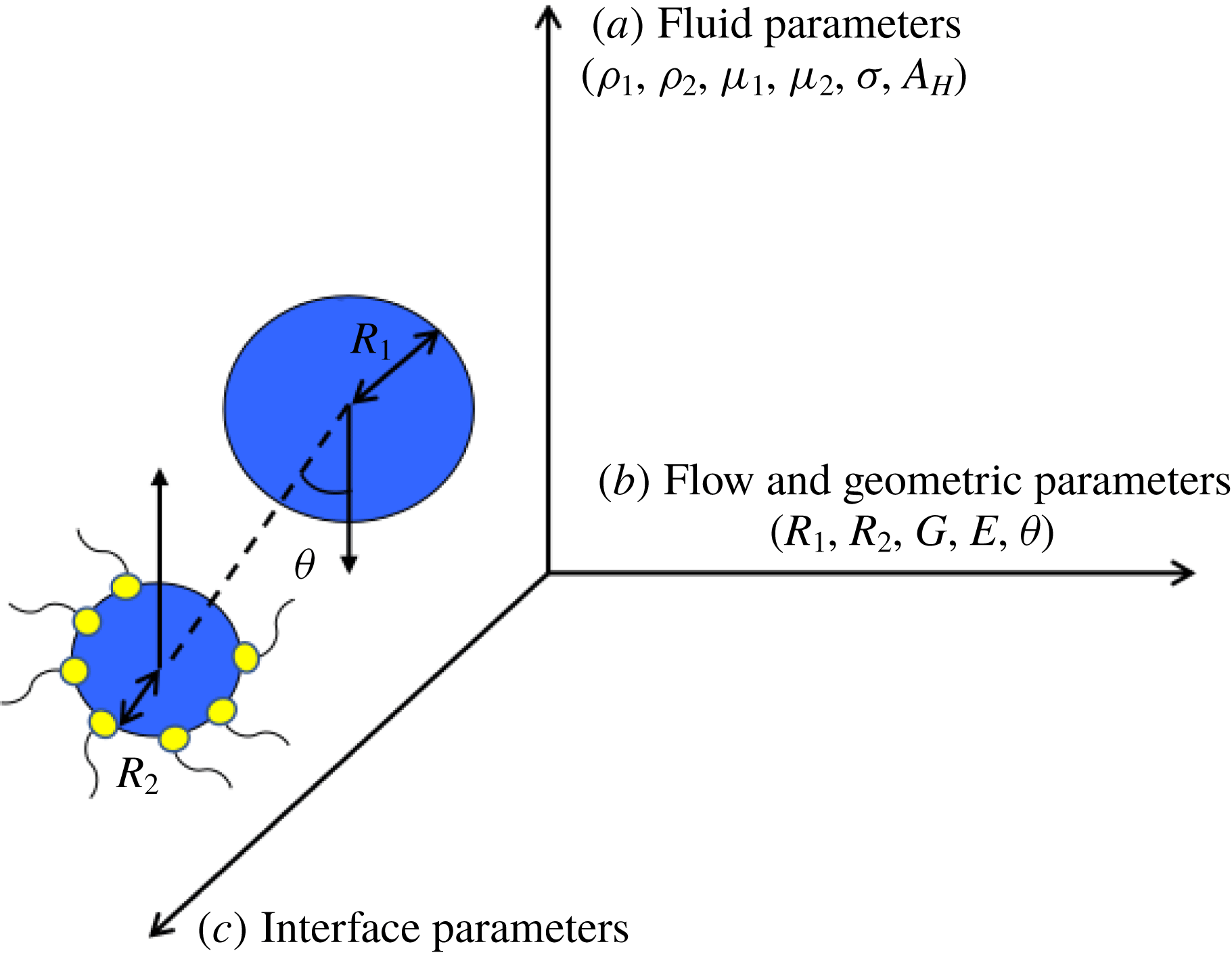
The pre-coalescence dynamics of a drop pair consists of three steps. First, the two drops approach each other due to a driving force, which can be the gravitational or buoyancy force among others, or due to an imposed flow of the external (also referred to as the exterior or outer or ambient) fluid. As the drops get closer, the thin film of the outer liquid that forms between the approaching drops begins to drain. Finally, once the film thickness falls below some critical value, van der Waals forces of attraction destabilize and rupture the film, leading to coalescence of the drops (Chesters Reference Chesters1991). The parameters influencing this process, shown in figure 1, can be broadly categorized as: (i) fluid parameters (for Newtonian fluids, these include the densities of the inner and outer liquids
 $\unicode[STIX]{x1D70C}_{1}$
and
 $\unicode[STIX]{x1D70C}_{2}$
, their respective viscosities
 $\unicode[STIX]{x1D707}_{1}$
and
 $\unicode[STIX]{x1D707}_{2}$
, the surface or interfacial tension of the interface separating the two liquids
 $\unicode[STIX]{x1D70E}$
and the Hamaker constant
 $A_{H}$
for the system), (ii) flow and geometric parameters (such as the radii
 $R_{1}$
and
 $R_{2}$
of the two drops, the strain rate of the imposed flow
 $G$
, the strength of the electric field
 $E$
driving the two drops together and the offset of the approaching drops
 $\unicode[STIX]{x1D703}$
) and (iii) interfacial rheological effects or interface parameters over and above the constant interfacial tension that is typically sufficient to characterize clean interfaces (such as surfactant concentration and/or charge distribution along the interface). Extensive experimental studies of flow-induced coalescence in the Stokes limit of two equal-sized drops in a four-roll Taylor mill set-up (Taylor Reference Taylor1934) have been conducted by Leal and coworkers (Yang et al.
Reference Yang, Park, Hu and Leal2001; Borrell, Yoon & Leal Reference Borrell, Yoon and Leal2004; Leal Reference Leal2004; Yoon et al.
Reference Yoon, Borrell, Park and Leal2005; Hsu, Roy & Leal Reference Hsu, Roy and Leal2008). Through these experiments, these authors have observed that the dependence of drainage time
 $\tilde{t}_{d}$
– defined as the time elapsed between the instant when the centre-to-centre distance
 $\tilde{d}$
between the drops is twice their undeformed radius
 $R$
to when the drops make contact – on the capillary number
 $Ca$
in a head-on collision (as seen in figure 2
a) can be described by the scaling relation
 $\tilde{t}_{d}G\sim Ca^{m}$
. Here,
 $G$
is the strain rate of the imposed compressional flow in the outer liquid and
 $Ca\equiv \unicode[STIX]{x1D707}_{2}GR/\unicode[STIX]{x1D70E}$
, where
 $\unicode[STIX]{x1D707}_{2}$
is the viscosity of the outer liquid. For large
 $Ca$
or, equivalently, large drops of
 $R>27$
 $\unicode[STIX]{x1D707}$
m, Leal and coworkers have shown that
 $m=4/3$
, which agrees with the theoretically expected prediction for the drainage of a flat or a dimpled film (Frostad, Walter & Leal Reference Frostad, Walter and Leal2013). For lower capillary numbers, the value of the exponent
 $m$
lies in the range
 $1<m<4/3$
, as the drops are observed to remain virtually spherical until coalescence (Hsu et al.
Reference Hsu, Roy and Leal2008).
A cartoon of the three-dimensional space of parameters affecting the collision and coalescence of two drops. These parameters can be broadly categorized as (a) fluid parameters or properties, (b) flow and geometric parameters and (c) interface parameters or properties. For illustration purposes, surfactant molecules are shown to populate the interface of the drop of radius
 $R_{2}$
.

While experimental techniques provide insights into macroscopic features of drop coalescence, analytical and numerical methods are essential for understanding the drainage of the film between the drops and establishing the mechanisms that are involved. Davis and coworkers (Yiantsios & Davis Reference Yiantsios and Davis1991; Davis Reference Davis1999) have focused on the drainage of the film for gravity-driven coalescence of drops, and made use of the lubrication approximation while solving the Navier–Stokes equations. Later, three-dimensional boundary integral methods were used by Rother, Zinchenko & Davis (Reference Rother, Zinchenko and Davis1997), Zinchenko, Rother & Davis (Reference Zinchenko, Rother and Davis1997) and Rother & Davis (Reference Rother and Davis2001) to study the effect of local deformations on two drops colliding in linear flows. Yue et al. (Reference Yue, Feng, Liu and Shen2005) used diffuse interface methods to study the coalescence dynamics of drops imparted with initial velocities directed at each other. Loewenberg and coworkers (Nemer et al.
Reference Nemer, Chen, Papadopoulos, Blawzdziewicz and Loewenberg2004, Reference Nemer, Chen, Papadopoulos, Blawzdziewicz and Loewenberg2007) showed that the external flow field affects the flow inside the drops which could arrest film drainage and as a result prevent coalescence, thereby demonstrating the contrast between drops coalescing due to an external flow field and drops pushed together by body forces in a quiescent fluid. Janssen et al. (Reference Janssen, Anderson, Peters and Meijer2006) and Yoon et al. (Reference Yoon, Baldessari, Ceniceros and Leal2007) derived simple scaling relations for the scaled drainage time
 $\tilde{t}_{d}G$
with
 $Ca$
and observed good agreement for scaling behaviour of drainage times between their boundary integral simulations and the experiments conducted by Leal and coworkers for large
 $Ca$
. Recently, Nemer et al. (Reference Nemer, Santoro, Chen, Bławzdziewicz and Loewenberg2013) derived scaling relationships for the variation of film thickness with time when the drops undergo small deformations. More recently, Ramachandran & Leal (Reference Ramachandran and Leal2016) examined the impact of interfacial slip on scaling exponents for film drainage times in an effort to resolve discrepancies in experimentally observed trends and simple scaling theories for smaller
 $Ca$
.
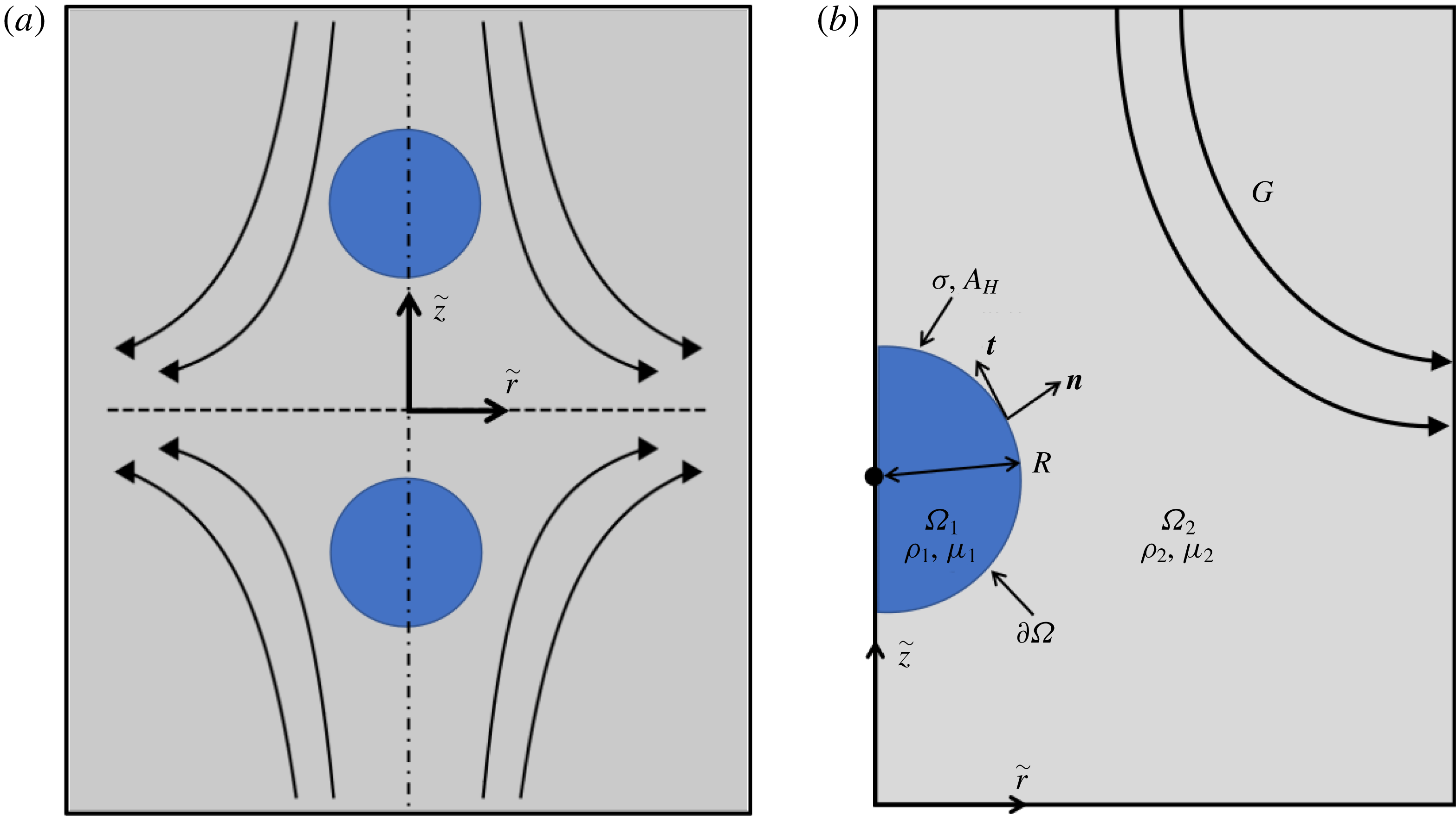
(a) Definition sketch for head-on collision of two equal-sized drops of a Newtonian liquid immersed in a second Newtonian liquid that are driven towards each other by a compressional flow similar to that in Taylor’s four-roll mill apparatus (Taylor Reference Taylor1934). (b) Sketch showing the problem domain corresponding to a quadrant of the
 $(\tilde{r},\tilde{z})$
-plane and the key problem variables.

While these aforementioned works have focused on highly viscous systems such that their dynamics lies in the Stokes regime, the hydrodynamics of the coalescence of slightly to moderately viscous systems such as water–oil emulsions may not conform to the assumptions of Stokes flow and hence require accounting for inertial effects. Controlled experiments on colliding liquid drops surrounded by a second liquid when inertia is non-negligible or at finite Reynolds number
 $Re$
are currently lacking. Moreover, previous computational works that have considered inertial effects (Nobari, Jan & Tryggvason Reference Nobari, Jan and Tryggvason1996) have not captured well the actual drainage and rupture dynamics of the film leading to coalescence. Indeed, it has proven challenging in previous computational studies to fully resolve the dynamics of the thin film separating two approaching drops given the multi-scale nature of the problem. For example, Thomas, Esmaeeli & Tryggvason (Reference Thomas, Esmaeeli and Tryggvason2010) state that ‘These films can become very thin and in direct numerical simulations (DNS) it is often impractical to resolve their thickness fully, even with adaptive grid refining’. The need to include inertial effects in modelling drop coalescence has eloquently been highlighted in a recent review article by Janssen & Anderson (Reference Janssen and Anderson2011). With the goal of accounting for inertial effects while accurately capturing the dynamics of interface rupture, we formulate and solve numerically in this paper the problem of the flow-induced approach, collision and eventual coalescence of two drops in an outer liquid at finite
 $Re$
.
This paper is organized as follows. Section 2 describes in detail the problem being studied and summarizes the equations as well as the boundary and initial conditions that govern the dynamics of drop coalescence. Section 3 describes the computational methods employed to solve numerically the aforementioned equations and presents the results of validation tests conducted to verify the accuracy of these methods. Section 4 presents the results obtained by solving the governing equations and examines the role that fluid inertia plays in causing two approaching drops to rebound and thereby result in an increase in film drainage times. Section 5 concludes the paper by summarizing the key results and discussing future avenues that can be explored by extending the current analyses.
2 Mathematical formulation
2.1 Governing equations and boundary and initial conditions
The system consists of two initially spherical drops of equal radii
 $R$
of an incompressible Newtonian liquid of constant density
 $\unicode[STIX]{x1D70C}_{1}$
and constant viscosity
 $\unicode[STIX]{x1D707}_{1}$
, suspended in an immiscible, incompressible Newtonian liquid of constant density
 $\unicode[STIX]{x1D70C}_{2}$
and constant viscosity
 $\unicode[STIX]{x1D707}_{2}$
. The interfacial tension of the liquid–liquid interface is spatially uniform and constant in time and is denoted by
 $\unicode[STIX]{x1D70E}$
, while the Hamaker constant for the liquid–liquid system
 $A_{H}$
is constant and positive, signifying that the force between the drops is attractive. The drops are initially separated by a centre-to-centre distance
 $\tilde{d}(\tilde{t}=0)=\unicode[STIX]{x1D6FC}R$
, where
 $\tilde{t}$
is time and the constant
 $4<\unicode[STIX]{x1D6FC}<\infty$
, and pushed towards each other by a compressional flow with a constant strain rate
 $G$
, identical to that generated by a four-roll Taylor mill (Taylor Reference Taylor1934). It proves convenient to adopt a cylindrical coordinate system where the origin is located midway between the two drops along the line connecting their centres;
 $\tilde{r}$
and
 $\tilde{z}$
represent the radial and axial coordinates, and
 $\boldsymbol{e}_{r}$
and
 $\boldsymbol{e}_{z}$
are the orthogonal unit vectors in the radial and axial directions in the cylindrical coordinate system used. The problem domain is reduced to one quadrant owing to axisymmetry about the axis
 $\tilde{r}=0$
and symmetry about the plane
 $\tilde{z}=0$
. A detailed schematic is shown in figure 2. In what follows, the subscript
 $()_{i}$
denotes variables in the drop when
 $i=1$
and variables in the outer liquid when
 $i=2$
.
In this paper, problem variables are non-dimensionalized using the undeformed drop radius
 $R$
as the characteristic length
 $l_{c}\equiv R$
, the inertial–capillary time scale (based on the drop density) as the characteristic time
 $t_{c}\equiv \sqrt{\unicode[STIX]{x1D70C}_{1}R^{3}/\unicode[STIX]{x1D70E}}$
, the ratio of the two, which is the inertial–capillary velocity, as the characteristic velocity scale
 $v_{c}\equiv l_{c}/t_{c}=\sqrt{\unicode[STIX]{x1D70E}/\unicode[STIX]{x1D70C}_{1}R}$
and the capillary pressure as the characteristic stress
 $p_{c}\equiv \unicode[STIX]{x1D70E}/R$
. The flow is then governed by the following dimensionless groups: the Ohnesorge number
 $Oh=\unicode[STIX]{x1D707}_{1}/\sqrt{\unicode[STIX]{x1D70C}_{1}\unicode[STIX]{x1D70E}R}$
, which is the ratio of the viscous force to the square root of the product of the inertial and capillary forces, viscosity ratio
 $m_{2}=\unicode[STIX]{x1D707}_{2}/\unicode[STIX]{x1D707}_{1}$
, density ratio
 $\unicode[STIX]{x1D6FE}_{2}=\unicode[STIX]{x1D70C}_{2}/\unicode[STIX]{x1D70C}_{1}$
, dimensionless strain rate
 $U_{\infty }=G\sqrt{\unicode[STIX]{x1D70C}_{1}R^{3}/\unicode[STIX]{x1D70E}}$
(which can also be thought of as the ratio of the imposed velocity
 $RG$
to the inertial–capillary velocity
 $v_{c}$
) and the van der Waals number
 $A=A_{H}/(6\unicode[STIX]{x03C0}\unicode[STIX]{x1D70E}R^{2})$
which is the ratio of the force due to van der Waals attraction to capillary force. In what follows, variables without tildes over them denote the dimensionless counterparts of the variables with tildes over them, e.g.
 $\tilde{r}$
and
 $r\equiv \tilde{r}/R$
stand for the dimensional and the dimensionless radial coordinate.
The dynamics in the regions
 $\unicode[STIX]{x1D6FA}_{1}(t)$
and
 $\unicode[STIX]{x1D6FA}_{2}(t)$
, i.e. inside and outside the drops, is governed by the continuity and Navier–Stokes equations which are given in dimensionless form by
 $$\begin{eqnarray}\displaystyle & \displaystyle \unicode[STIX]{x1D735}\boldsymbol{\cdot }\boldsymbol{v}_{i}=0 & \displaystyle\end{eqnarray}$$
 $$\begin{eqnarray}\displaystyle & \displaystyle \unicode[STIX]{x1D6FE}_{i}\left(\frac{\unicode[STIX]{x2202}\boldsymbol{v}_{i}}{\unicode[STIX]{x2202}t}+\boldsymbol{v}_{i}\boldsymbol{\cdot }\unicode[STIX]{x1D735}\boldsymbol{v}_{i}\right)=\unicode[STIX]{x1D735}\boldsymbol{\cdot }\unicode[STIX]{x1D64F}_{i}, & \displaystyle\end{eqnarray}$$
 $\unicode[STIX]{x1D64F}_{i}\equiv -p_{i}\boldsymbol{I}+m_{i}Oh[(\unicode[STIX]{x1D735}\boldsymbol{v}_{i})+(\unicode[STIX]{x1D735}\boldsymbol{v}_{i})^{T}]$
, and
 $p_{i}$
and
 $\boldsymbol{v}_{i}=u_{i}\boldsymbol{e}_{r}+w_{i}\boldsymbol{e}_{z}$
denote the pressure and velocity in liquid
 $i$
respectively. Furthermore,
 $u_{i}$
and
 $w_{i}$
stand for the radial and axial components of the fluid velocity. Lastly, the density and viscosity ratios for fluid
 $1$
are used as characteristic values such that
 $\unicode[STIX]{x1D6FE}_{1}=m_{1}=1$
, while
 $\unicode[STIX]{x1D6FE}_{2}$
and
 $m_{2}$
have already been specified.
The governing equations are solved subject to a number of boundary conditions. Key among these are the kinematic and traction boundary conditions that are applied at the liquid–liquid interface
 $\unicode[STIX]{x2202}\unicode[STIX]{x1D6FA}(t)$
, which is unknown a priori, to enforce mass conservation and account for the jump in stress due to interfacial tension and van der Waals forces
 $$\begin{eqnarray}\displaystyle & \displaystyle \boldsymbol{n}\boldsymbol{\cdot }(\boldsymbol{v}_{i}-\boldsymbol{v}_{s})=0, & \displaystyle\end{eqnarray}$$
 $$\begin{eqnarray}\displaystyle & \displaystyle \boldsymbol{n}\boldsymbol{\cdot }(\unicode[STIX]{x1D64F}_{2}-\unicode[STIX]{x1D64F}_{1})=2H\boldsymbol{n}-\frac{A}{h^{3}}\boldsymbol{n}, & \displaystyle\end{eqnarray}$$
 $\boldsymbol{n}$
represents the unit normal to the interface as shown in figure 2,
 $\boldsymbol{v}_{s}$
represents the velocity of points on the interface and
 $2H$
represents twice the mean curvature, equal to minus the surface divergence of the unit normal
 $(-\unicode[STIX]{x1D735}_{s}\boldsymbol{\cdot }\boldsymbol{n})$
. The second term on the right side of (2.2b
) represents van der Waals attraction between the two drops which becomes significant when the axial distance between the interfaces, denoted by
 $h\equiv \tilde{h}/R$
, becomes of the order of a few hundred nanometres, and thus the value of
 $A$
is typically small (De Gennes Reference De Gennes1985; Teletzke, Davis & Scriven Reference Teletzke, Davis and Scriven1987; Chesters Reference Chesters1991). In the current formulation,
 $h/2\equiv \tilde{h}/2R$
is taken to be equal to the axial coordinate of the interface
 $\unicode[STIX]{x2202}\unicode[STIX]{x1D6FA}(t)$
. It should be noted that in the current formulation as has also been the case in virtually all other studies involving drop coalescence and the rupture of thin films and liquid sheets, the effects of interface curvature on van der Waals forces are neglected. As shown by Dai, Leal & Redondo (Reference Dai, Leal and Redondo2008), the complete expression for the disjoining pressure leads to corrections of the order of
 $(\tilde{h}/R)^{2}$
to the original expression derived for plane interfaces. As van der Waals forces become significant when
 $\tilde{h}/R\approx 10^{-4}$
(see below), we are justified in neglecting curvature effects, which are tantamount to corrections of the order of
 $10^{-8}$
compared to the order-one term used in our problem formulation.
Additional boundary conditions arise because of symmetry and the far field condition on the velocity at large distances from the two drops. Symmetry boundary conditions are applied at the axis of (axi)symmetry
 $r=0$
and the plane of symmetry
 $z=0$
. At large distances from the origin, the velocity field in the outer liquid
 $\boldsymbol{v}_{2}$
is given by
 $$\begin{eqnarray}\boldsymbol{v}_{2}(|\boldsymbol{x}|\rightarrow \infty )=U_{\infty }\left(\frac{r}{2}\boldsymbol{e}_{r}-z\boldsymbol{e}_{z}\right),\end{eqnarray}$$
where
 $\boldsymbol{x}$
is the position vector.
The system is initially quiescent and two stationary, equal-sized, spherical drops are separated by a dimensionless centre-to-centre distance
 $d(t=0)=\unicode[STIX]{x1D6FC}$
. At time
 $t=0$
, the flow in the outer liquid is impulsively turned on by imposing the velocity profile given by (2.3) and maintained at that value thereafter to drive the two drops toward each other.
2.2 Choice and values of dimensionless groups
On account of the different characteristic scales used in this paper and those employed by previous researchers to simulate drop coalescence under creeping flow conditions (Janssen et al.
Reference Janssen, Anderson, Peters and Meijer2006; Yoon et al.
Reference Yoon, Baldessari, Ceniceros and Leal2007; Nemer et al.
Reference Nemer, Santoro, Chen, Bławzdziewicz and Loewenberg2013), it is useful to relate the dimensionless groups used here to the capillary number
 $Ca$
and Reynolds number
 $Re$
used by others,
 $$\begin{eqnarray}\displaystyle & \displaystyle Ca=\frac{\unicode[STIX]{x1D707}_{2}GR}{\unicode[STIX]{x1D70E}}=m_{2}OhU_{\infty }, & \displaystyle\end{eqnarray}$$
 $$\begin{eqnarray}\displaystyle & \displaystyle Re=\frac{\unicode[STIX]{x1D70C}_{2}(GR)R}{\unicode[STIX]{x1D707}_{2}}=\frac{U_{\infty }\unicode[STIX]{x1D6FE}_{2}}{m_{2}Oh}. & \displaystyle\end{eqnarray}$$
In these previous publications, both of these dimensionless groups are defined using the properties of the outer liquid (the middle terms in the previous two equations), as opposed to the practice adopted here, where the properties of the drop liquid are used as characteristic values. It is worth noting that whereas
 $U_{\infty }=Gt_{c}=(GR)/(R/t_{c})$
is the ratio of the imposed velocity to the inertial–capillary velocity,
 $OhU_{\infty }=Gt_{v}=(GR)/(R/t_{v})$
is the ratio of the imposed velocity to the visco-capillary velocity where
 $t_{v}=\unicode[STIX]{x1D707}_{1}R/\unicode[STIX]{x1D70E}$
is the visco-capillary time (based on the drop viscosity). Also, the Ohnesorge number can then be seen to be the ratio of the two capillary time scales, viz.
 $Oh=t_{v}/t_{c}$
. It is clear that in the creeping flow limit,
 $Oh\rightarrow \infty$
and
 $U_{\infty }\rightarrow 0$
while
 $OhU_{\infty }$
and hence
 $Ca$
are finite but because
 $U_{\infty }/Oh=Gt_{c}^{2}/t_{v}$
, both
 $U_{\infty }/Oh$
and
 $Re\rightarrow 0$
as can be seen from (2.4) and (2.5). Therefore, later in the paper, the values of
 $U_{\infty }$
and
 $Oh$
can be varied in a such a way that the product
 $OhU_{\infty }$
can be kept constant to match capillary numbers used in earlier studies but the ratio
 $U_{\infty }/Oh$
can be systematically increased from a small value to probe the effect of increasing inertia on the coalescence dynamics.
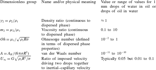
Values of key dimensionless groups used in the simulations.

In addition to retaining some similarity between the values of certain dimensionless groups used here with earlier studies, the range of values of the dimensionless groups used in the simulations was dictated by focusing attention on one of the most important practical applications of coalescence. This application concerns oil–water and water–oil emulsions which arise in the processing of crude oil or petroleum among others. Table 1 lists the ranges of the values of the dimensionless groups in such systems composed of drops of radii of 1 mm (or
 $10^{-3}$
m). In arriving at the values of the parameters in this table, use was made of the fact that in such systems and in most liquid–liquid emulsions, the densities of both phases are approximately
 $1~\text{g}~\text{cm}^{-3}$
(or
 $10^{3}~\text{kg}~\text{m}^{-3}$
) so that
 $\unicode[STIX]{x1D6FE}_{2}\approx 1$
. The interfacial tension of most liquid–liquid systems is of the order of ten to tens of
 $\text{dyne}~\text{cm}^{-1}$
(or
 $\text{mN}~\text{m}^{-1}$
). Thus, taking a nominal value of
 $\unicode[STIX]{x1D70E}=10~\text{dyne}~\text{cm}^{-1}$
,
 $Oh=\unicode[STIX]{x1D707}_{1}/\sqrt{(1)(10^{-1})(10)}=\unicode[STIX]{x1D707}_{1}$
if cgs units are used. Thus, if the dispersed phase is water,
 $Oh=10^{-2}$
, but if it is crude oil,
 $10^{-2}\leqslant Oh\leqslant 0.1$
to 1. Therefore, for most water and oil emulsions, the viscosity ratio
 $m_{2}$
ranges between 0.1 and 10. Also, we do not consider values of
 $m_{2}$
smaller than 0.1 and larger than 10 because in a scaling or order of magnitude analysis, values that are small, order one, and large correspond to 0.1, 1 and 10 (Deen Reference Deen1998). Values of the van der Waals number are based on standard values of the Hamaker constant which lies between
 $10^{-21}$
and
 $10^{-18}$
J. For drops of radii of 1 mm,
 $Re=G(10^{-1})^{2}(1)/\unicode[STIX]{x1D707}_{2}$
in cgs units. Therefore, to obtain a Reynolds number of unity,
 $G=1~\text{s}^{-1}$
if the external phase is water or a low-viscosity crude oil but
 $G=10~\text{s}^{-1}$
if the external phase is a crude oil that is ten times more viscous than water. For 1 mm drops, the inertial–capillary time is
 $10^{-2}$
s. The aforementioned values of
 $G$
correspond to values of
 $U_{\infty }$
of
 $10^{-2}$
and
 $10^{-1}$
. Thus, in many simulations reported later on in the paper, a value of
 $U_{\infty }=0.05$
is used.
In this paper, the effect of gravity on the coalescence dynamics is neglected. The velocity of rise/fall of a spherical drop to buoyancy is known to scale as
 $u_{b}\sim |\unicode[STIX]{x0394}\unicode[STIX]{x1D70C}|gR^{2}/\unicode[STIX]{x1D707}_{2}$
where
 $\unicode[STIX]{x0394}\unicode[STIX]{x1D70C}\equiv \unicode[STIX]{x1D70C}_{2}-\unicode[STIX]{x1D70C}_{1}$
and
 $g$
is the acceleration due to gravity. Thus, the effect of gravity is negligible if
 $u_{b}$
is small compared to the imposed velocity
 $GR$
or
 $$\begin{eqnarray}\frac{u_{b}}{GR}\sim Bo/Ca\ll 1,\end{eqnarray}$$
where
 $Bo=|\unicode[STIX]{x0394}\unicode[STIX]{x1D70C}|gR^{2}/\unicode[STIX]{x1D70E}$
is the gravitational Bond number. Thus, when the densities of the two phases are identical so that
 $Bo=0$
, this inequality is always satisfied. For example, near the end of the results section, a phase diagram of coalescence is presented that shows how the drainage time varies with
 $Oh$
and
 $m_{2}$
when
 $\unicode[STIX]{x0394}\unicode[STIX]{x1D70C}=0$
. Situations when this inequality is not satisfied under terrestrial conditions can be considered to represent experiments in which coalescence between two drops takes place in a low-gravity environment (Wang et al.
Reference Wang, Anilkumar, Lee and Lin1994, Reference Wang, Trinh, Croonquist and Elleman1986).
3 Numerical solution scheme and validation tests
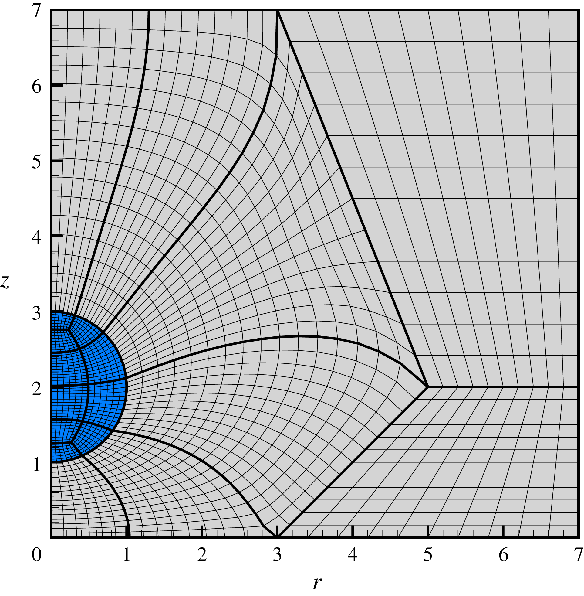
An illustrative coarse mesh that has been generated using the coupled elliptic–algebraic mesh generation algorithm that is used to tessellate the computational domain. The computational domain which, because of axial symmetry about
 $r=0$
and reflective symmetry about the plane
 $z=0$
, consists of one quadrant in the
 $(r,z)$
-plane and can be seen to have been divided into 18 quadrilateral sub-domains. Each of these sub-domains is then discretized using elliptic mesh generation for those sub-domains adjacent to the interface and typically algebraic mesh generation for ones far away from it. The mesh is weighted radially in regions where there are liquid–liquid interfaces to better capture the interface dynamics for a given computational cost.

The governing equations (2.1a
)–(2.1b
), subject to the interfacial boundary conditions (2.2a
)–(2.2b
), the remaining boundary conditions given in the previous section and the aforementioned initial conditions, for simulating the collision and coalescence of two drops suspended in a second liquid constitute a coupled set of transient nonlinear, second-order partial differential equations in space. These equations are solved by a fully implicit method of lines algorithm which utilizes an arbitrary Lagrangian–Eulerian scheme, the Galerkin finite element method for spatial discretization (Basaran & Wohlhuter Reference Basaran and Wohlhuter1992; Feng & Basaran Reference Feng and Basaran1994; Gresho & Sani Reference Gresho and Sani1998; Gockenbach Reference Gockenbach2006) and an adaptive finite difference method for time integration (Patzek et al.
Reference Patzek, Benner, Basaran and Scriven1991; Wilkes & Basaran Reference Wilkes and Basaran2001; Gockenbach Reference Gockenbach2006). As this problem is a free boundary problem that involves deformable liquid–liquid interfaces, a special elliptic mesh generation technique, originally developed for study of coating flows by Christodoulou & Scriven (Reference Christodoulou and Scriven1992) and later adapted to analyse transient free surface flows involving finite-time hydrodynamic singularities (see below), along with algebraic meshing techniques, is employed to track the moving boundaries and tessellate the moving/deforming domains (
 $\unicode[STIX]{x1D6FA}_{1}(t)\cup \unicode[STIX]{x1D6FA}_{2}(t)$
) into quadrilateral sub-domains (Notz & Basaran Reference Notz and Basaran2004). At each time step, the resulting nonlinear algebraic equations are solved iteratively using Newton’s method where the Jacobian is computed analytically. Complete formulation of residuals and corresponding Jacobians are given in Sambath (Reference Sambath2013), and additional details on computational methods used can be found in Sambath (Reference Sambath2013) and Garg (Reference Garg2018).
As it is impracticable in simulations for the computational domain in the exterior liquid to extend all the way out to infinity, the domain is truncated at a radial location
 $r=r_{\infty }$
and axial location
 $z=z_{\infty }$
, and where boundary condition (2.3) is imposed. For all the results to be presented in this paper,
 $r_{\infty }=z_{\infty }=7$
. Further systematic increases to the values of these distances resulted in negligible changes in the computed results. Moreover, with the exception of one case, in all of the simulation results to be reported, the initial centre-to-centre separation between the drops was taken to equal four times the drop radii, viz.
 $d(t=0)=\unicode[STIX]{x1D6FC}=4$
. Systematic grid independence studies were also carried out to determine discretizations that are needed to yield mesh-independent results. A sample coarse mesh is shown in figure 3. Newton iterations, which were continued until residual norms fell below
 $10^{-6}$
, were found to converge quadratically, thereby confirming the correctness of the analytically computed Jacobian. Typically, 3–4 iterations were required to attain convergence at each time step. Variants of this algorithm have been well benchmarked and used by our group in the past to analyse hydrodynamic singularities that arise during the breakup of filaments (Chen, Notz & Basaran Reference Chen, Notz and Basaran2002; Notz & Basaran Reference Notz and Basaran2004; Suryo & Basaran Reference Suryo and Basaran2006; Bhat et al.
Reference Bhat, Appathurai, Harris, Pasquali, McKinley and Basaran2010; Thete et al.
Reference Thete, Anthony, Basaran and Doshi2015; Castrejón-Pita et al.
Reference Castrejón-Pita, Castrejón-Pita, Thete, Sambath, Hutchings, Hinch, Lister and Basaran2015; Kamat et al.
Reference Kamat, Wagoner, Thete and Basaran2018), rupture of thin films (Garg et al.
Reference Garg, Kamat, Anthony, Thete and Basaran2017) and breakup and coalescence of bubbles (Munro et al.
Reference Munro, Anthony, Basaran and Lister2015; Anthony et al.
Reference Anthony, Kamat, Thete, Munro, Lister, Harris and Basaran2017) and drops (Paulsen et al.
Reference Paulsen, Burton, Nagel, Appathuri, Harris and Basaran2012; Collins et al.
Reference Collins, Sambath, Harris and Basaran2013).
To validate the code that has been developed and used in this paper, predictions that are made with it are tested against well-established results in the literature on linear stability analysis of the oscillations of liquid drops that are surrounded by another liquid when inertial (viscous) effects are dominant (negligible), and experimental and computational studies of drop coalescence when viscous (inertial) effects are dominant (negligible).
Rayleigh (Reference Rayleigh1879) obtained the frequencies
 $\unicode[STIX]{x1D714}_{R}$
of small-amplitude, axisymmetric oscillations of an incompressible, inviscid liquid drop that is freely suspended in a second immiscible incompressible, inviscid liquid. During linear oscillations, a drop whose undisturbed profile is a sphere undergoes shape oscillations such that the
 $n$
th mode of oscillation and hence the perturbation to the spherical base profile is proportional to the Legendre polynomial of order
 $n$
,
 $P_{n}(\cos \unicode[STIX]{x1D703})$
, where
 $\unicode[STIX]{x1D703}$
is the azimuthal angle measured from the axis of symmetry and
 $n\geqslant 2$
. In dimensionless form, the dispersion relation obtained by Rayleigh (Reference Rayleigh1879) that gives the eigenfrequency of each linear mode of oscillation is
 $$\begin{eqnarray}\unicode[STIX]{x1D714}_{R}(n,\unicode[STIX]{x1D6FE}_{2})=\left[\frac{n(n-1)(n+1)(n+2)}{(n+1)+n\unicode[STIX]{x1D6FE}_{2}}\right]^{1/2}.\end{eqnarray}$$
Almost a century later, Miller & Scriven (Reference Miller and Scriven1968) (see also Prosperetti (Reference Prosperetti1980), Marston (Reference Marston1980) and Basaran, Scott & Byers (Reference Basaran, Scott and Byers1989)) determined the corresponding linearized frequencies of oscillation when both liquids have finite viscosities. Although the form of the general dispersion equation is complex, it takes on a particularly simple form when both fluids have low viscosities. With this so-called low-viscosity approximation (LVA), the frequency of the
 $n$
th eigenmode of oscillation is given by
 $$\begin{eqnarray}\unicode[STIX]{x1D714}_{LVA}(n,\unicode[STIX]{x1D6FE}_{2})=\unicode[STIX]{x1D714}_{R}\left[1-\frac{(2n+1)^{2}\sqrt{Oh\unicode[STIX]{x1D6FE}_{2}}}{2\sqrt{2}(n+1+\unicode[STIX]{x1D6FE}_{2}n)(1+\sqrt{\unicode[STIX]{x1D6FE}_{2}})}\right].\end{eqnarray}$$
To compare predictions made with the code of this paper with exact results from linear theory given above, the code developed here was used to simulate the axisymmetric oscillations of a free liquid drop of low viscosity of
 $Oh=10^{-3}$
and
 $m_{2}=1$
over a range of density ratios
 $\unicode[STIX]{x1D6FE}_{2}$
. In the simulations, the drops were released from an initial static shape given by
 $f(\unicode[STIX]{x1D703},t=0)=1+\unicode[STIX]{x1D700}P_{2}(\cos \unicode[STIX]{x1D703})$
where the perturbation amplitude
 $\unicode[STIX]{x1D700}=0.1$
(Basaran Reference Basaran1992).
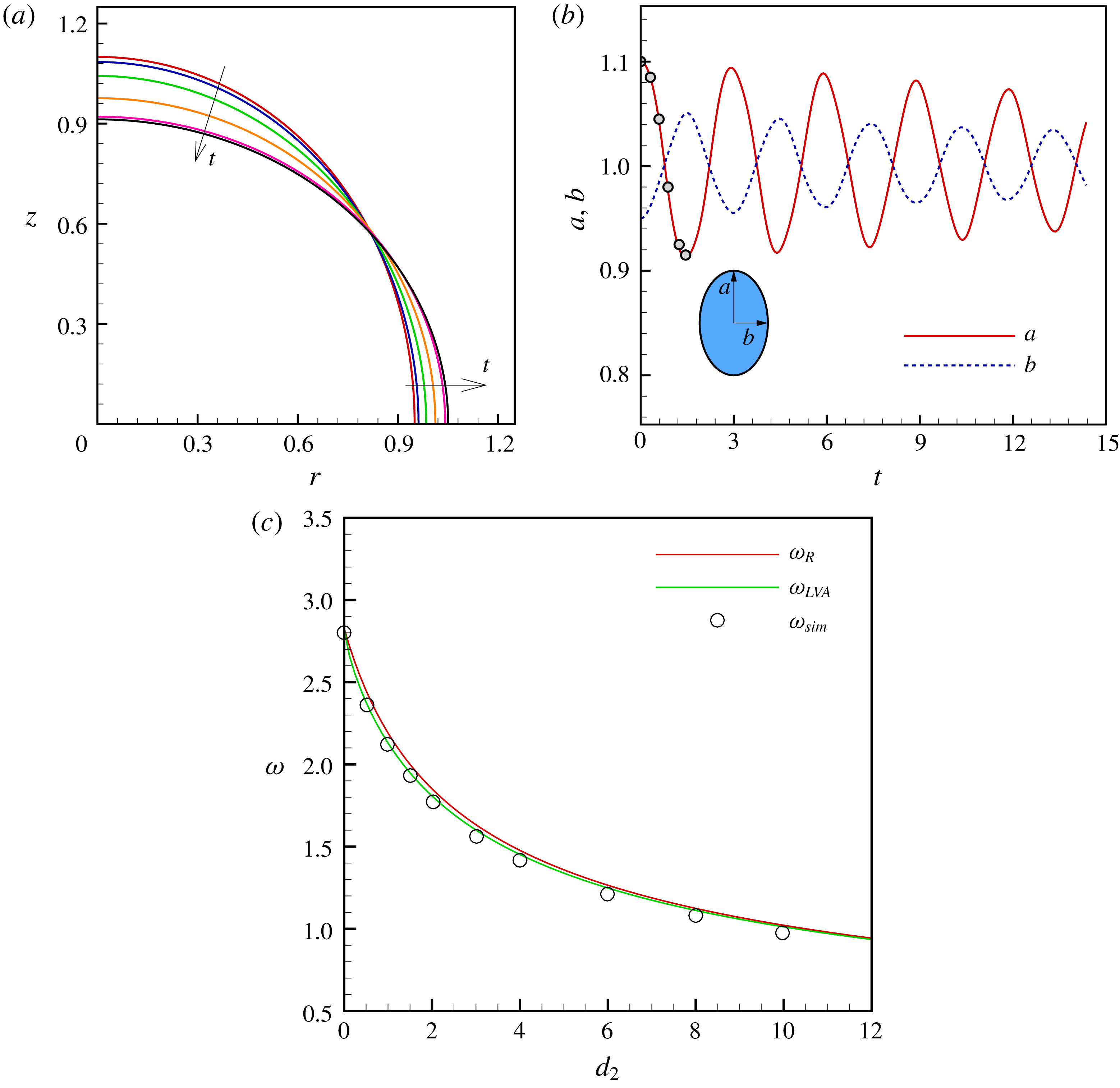
Transient shapes, half the major and minor axes and oscillation frequencies of a low-viscosity drop of
 $Oh=10^{-3}$
that is immersed in another low-viscosity liquid of the same viscosity as the drop (
 $m_{2}=1$
). In the simulations, the drops are released from static deformations such that the drop’s shape
 $f(\unicode[STIX]{x1D703},t=0)$
as a function of the meridional angle
 $\unicode[STIX]{x1D703}$
in spherical coordinates is given by
 $f(\unicode[STIX]{x1D703},t=0)=1+0.1P_{2}(\cos \unicode[STIX]{x1D703})$
. Computed (a) shapes at six instants in time and (b) variation in time of half the major axis
 $a$
and half the minor axis
 $b$
of a drop that is oscillating in an exterior liquid of the same density as the drop (
 $\unicode[STIX]{x1D6FE}_{2}=1$
). The profiles shown in (a) correspond to time instants of
 $t=0,0.3,0.6,0.9,1.2$
and 1.5, which are marked by circles in (b). (c) Variation of oscillation frequency with density ratio
 $\unicode[STIX]{x1D6FE}_{2}$
: comparison of frequencies obtained from simulations (
 $\unicode[STIX]{x1D714}_{sim}$
) with ones from the inviscid theory of Rayleigh (Reference Rayleigh1879) (
 $\unicode[STIX]{x1D714}_{R}$
) and the low-viscosity approximation of Miller & Scriven (Reference Miller and Scriven1968) (
 $\unicode[STIX]{x1D714}_{LVA}$
).

Figure 4(a) shows the instantaneous shapes of an oscillating drop of a low-viscosity liquid of
 $Oh=10^{-3}$
that is surrounded by a liquid of the same viscosity and density as the drop liquid, i.e.
 $m_{2}=1$
and
 $\unicode[STIX]{x1D6FE}_{2}=1$
, at six instants in time. Released from a prolate static deformation, the drop tends towards a sphere due to surface tension, overshoots its equilibrium position due to inertia and continues to oscillate about its equilibrium state. While these oscillations are eventually damped out, the computed value of the frequency of oscillations is expected to be close to that predicted by Rayleigh for an inviscid drop and by Miller and Scriven’s LVA because of the low value of
 $Oh=10^{-3}$
and smallness of the initial amplitude of the imposed perturbation. Figure 4(b) shows the evolution in time of the half-height
 $a$
of the drop along the symmetry or
 $z$
-axis and its radius
 $b$
in the equatorial plane, viz.
 $a/b$
is the drop’s instantaneous aspect ratio. The oscillatory response is virtually sinusoidal and the frequency of these oscillations, computed using the fast Fourier transform (FFT) method, is
 $\unicode[STIX]{x1D714}_{sim}=2.12$
. This value is within 4 % of
 $\unicode[STIX]{x1D714}_{R}=2.20$
predicted by Rayleigh’s inviscid theory from (3.1) but more reassuringly within 0.9 % of
 $\unicode[STIX]{x1D714}_{LVA}=2.14$
predicted by the more accurate viscous theory of Miller and Scriven from (3.2). Figure 4(c) shows excellent match between the frequencies obtained from simulations with those predicted from the inviscid theory of Rayleigh (Reference Rayleigh1879) and the low-viscosity approximation of Miller & Scriven (Reference Miller and Scriven1968) for situations in which
 $Oh$
and
 $m_{2}$
are held fixed but the density ratio
 $\unicode[STIX]{x1D6FE}_{2}$
is varied over a wide range. The excellent agreement observed between computed results and theoretical predictions provides credence to the accuracy of the code used in this work in simulating the dynamics of two-fluid flows when both fluids are nearly inviscid liquids or have low viscosities (Ohnesorge numbers).
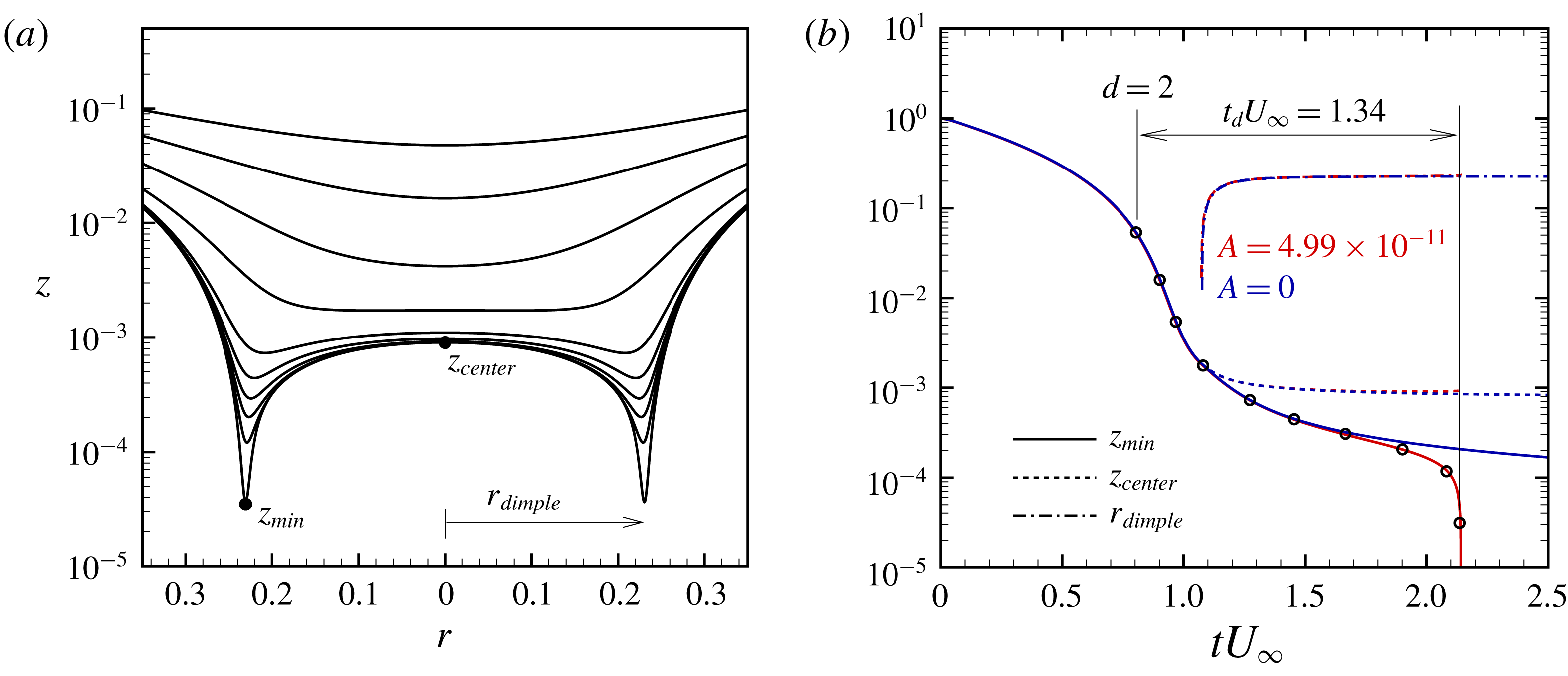
Computed evolution in time of (a) the shape of the liquid–liquid interface and (b) half the minimum axial separation between the drops
 $z_{min}$
, half the axial separation of the interfaces along the axis of symmetry
 $z_{centre}$
, and radius of the dimple
 $r_{dimple}$
that forms in mid to late stages of coalescence of two drops in an outer liquid. Here,
 $Oh=1.55\times 10^{4}$
,
 $m_{2}=5.33$
,
 $\unicode[STIX]{x1D6FE}_{2}=1.1$
,
 $U_{\infty }=1.81\times 10^{-7}$
and
 $A=4.99\times 10^{-11}$
(but see below). (It is worth noting from (2.4) and (2.5) that
 $Ca=0.015$
and
 $Re=1.3\times 10^{-12}$
.) In (b), simulation results are also shown for the situation in which all the dimensionless groups have the same values as before but the van der Waals force has been turned off (and hence the drops do not coalesce). The two cases are distinguished by drawing the curves corresponding to them in red and blue as indicated in (b). The open circles in (b) represent the time instants for which the shapes of the interface are shown in (a). In (b), the instant at which the centre-to-centre separation between the two drops equals twice their radii is identified by
 $d=2$
. The results of our simulations when
 $A\neq 0$
agree well with the simulations of Yoon et al. (Reference Yoon, Baldessari, Ceniceros and Leal2007). Moreover, the scaled drainage time
 $t_{d}U_{\infty }$
of 1.34 obtained from our simulations is in excellent agreement with the experimentally measured value of 1.32 of Yoon et al. (Reference Yoon, Borrell, Park and Leal2005) who studied coalescence of polybutylene (PB) drops suspended in polydimethysiloxane (PDMS).

Yoon et al. (Reference Yoon, Borrell, Park and Leal2005) experimentally investigated the coalescence dynamics of polybutylene (PB) drops suspended in polydimethylsiloxane (PDMS) using Taylor’s four-roll mill set-up and high speed imaging techniques. Two
 $27.2~\unicode[STIX]{x03BC}\text{m}$
drops of PB (
 $\unicode[STIX]{x1D70C}_{1}=890~\text{kg}~\text{m}^{-3}$
,
 $\unicode[STIX]{x1D707}_{1}=5.5~\text{Pa}~\text{s}$
) coalescing in PDMS (
 $\unicode[STIX]{x1D70C}_{2}=976~\text{kg}~\text{m}^{-3}$
,
 $\unicode[STIX]{x1D707}_{2}=29.3$
Pa s), where the interfacial tension between the two fluids was
 $\unicode[STIX]{x1D70E}=4.6\times 10^{-3}~\text{N}~\text{m}^{-1}$
, with a strain rate of
 $G=8.7\times 10^{-2}~\text{s}^{-1}$
had a scaled drainage time of
 $\tilde{t}_{d}G=1.32$
. (We note that
 $\tilde{t}_{d}G\equiv t_{d}U_{\infty }$
because
 $t_{d}\equiv \tilde{t}_{d}/t_{c}$
and
 $U_{\infty }\equiv Gt_{c}$
. Therefore, to avoid confusion, we refer to
 $t_{d}$
as the drainage time and
 $t_{d}U_{\infty }$
as the scaled drainage time.) These experimental results were later corroborated by the boundary integral simulations of Yoon et al. (Reference Yoon, Baldessari, Ceniceros and Leal2007) using the parameter values of
 $Ca=0.015$
,
 $m_{2}=5.33$
,
 $\unicode[STIX]{x1D6FE}_{2}=1.1$
and
 $A=4.99\times 10^{-11}$
. Figure 5 shows results of our simulation for the corresponding parameter values of
 $Oh=1.55\times 10^{4}$
,
 $m_{2}=5.33$
,
 $\unicode[STIX]{x1D6FE}_{2}=1.1$
,
 $U_{\infty }=1.81\times 10^{-7}$
and
 $A=4.99\times 10^{-11}$
. The time evolution of the shape of the liquid–liquid interface is shown in figure 5(a), and those of half of the minimum axial separation
 $z_{min}$
, half of the axial distance
 $z_{centre}$
between the two drops along the axis of symmetry, and the radius of the dimple
 $r_{dimple}$
are shown in figure 5(b). Our results exhibit excellent agreement with the simulations of Yoon et al. (Reference Yoon, Baldessari, Ceniceros and Leal2007), and yield a scaled drainage time of
 $\tilde{t}_{d}G\equiv t_{d}U_{\infty }=1.34$
which agrees closely with that measured experimentally by Yoon et al. (Reference Yoon, Borrell, Park and Leal2005) who had obtained a value of 1.32 (see above). (In all the simulation results presented in this paper, coalescence is said to occur when the minimum axial separation between the interfaces of the two drops
 $z_{min}$
falls below
 $5\times 10^{-6}$
. Thus, for two mm sized drops, coalescence occurs when their interfaces are separated by
 ${\sim}5$
nm.) The excellent accord between the new computational results and these well-established experimental and simulation results is further testament to the accuracy of the solution algorithm and computer code developed and used in this paper.
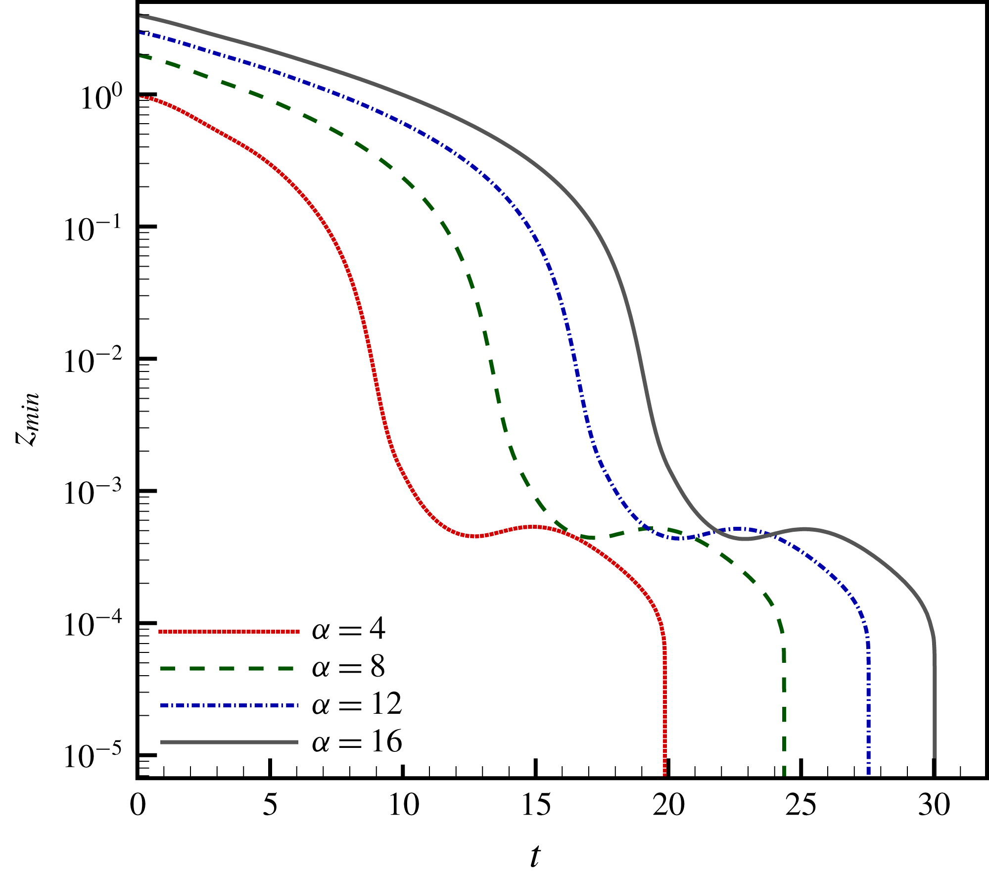
Computed evolution in time of half the minimum axial separation between the drops
 $z_{min}$
and resulting drainage times
 $t_{d}$
(see below) for four cases where all dimensionless groups are held constant while the initial separation between the drops
 $d(t=0)=\unicode[STIX]{x1D6FC}$
is successively increased by
 $4$
as indicated in the legend on the bottom left of the figure. The computed values of the drainage time are:
 $t_{d}=11.83$
when
 $\unicode[STIX]{x1D6FC}=4$
,
 $t_{d}=11.89$
when
 $\unicode[STIX]{x1D6FC}=8$
,
 $t_{d}=11.61$
when
 $\unicode[STIX]{x1D6FC}=12$
and
 $t_{d}=11.87$
when
 $\unicode[STIX]{x1D6FC}=16$
, thereby showing that
 $t_{d}$
remains virtually constant as the initial separation is varied by a factor of four. Here,
 $Oh=0.02$
,
 $m_{2}=5.26$
,
 $\unicode[STIX]{x1D6FE}_{2}=1.1$
,
 $U_{\infty }=0.095$
and
 $A=4.99\times 10^{-11}$
. It should be noted that for these parameter values,
 $Ca=0.01$
and
 $Re=1$
.

Before presenting the results of a detailed parametric study of drop coalescence, it is important to determine whether the initial separation between the centres of the two drops
 $d(t=0)=\unicode[STIX]{x1D6FC}$
has any effect on the drainage times to be reported in this paper. Figure 6 shows the computed evolution in time of half the minimum axial separation between the drops
 $z_{min}$
and resulting drainage times
 $t_{d}$
(see the caption to the figure) in four cases where the values of all the dimensionless groups except
 $\unicode[STIX]{x1D6FC}$
have been kept fixed and the value of
 $\unicode[STIX]{x1D6FC}$
has been successively increased by four. These results make plain that the drainage time
 $t_{d}$
is virtually independent of
 $\unicode[STIX]{x1D6FC}$
and that the only effect of increasing
 $\unicode[STIX]{x1D6FC}$
is to increase the time taken by the drops to reach a centre-to-centre separation of
 $d=2$
.
4 Results and discussion
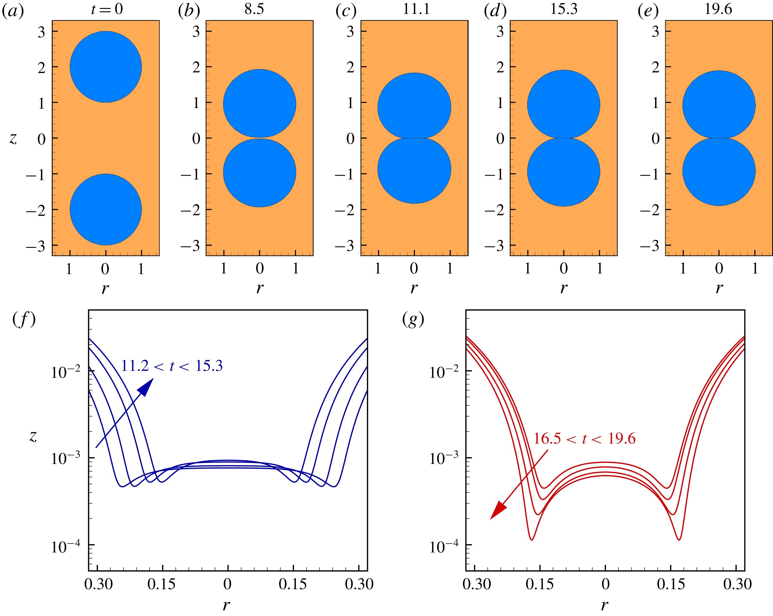
Time sequence of shapes and positions of two drops (a–e) and blow-ups of the interface shapes near coalescence (f–g). (a) The two drops at
 $t=0$
when their initial centre-to-centre separation is 4. Thereafter, the two drops are driven together by the imposed flow field in the external liquid. (b) As the drops get within one diameter of each other, their interfaces begin to deform forming a thin film of the surrounding liquid between them. (c–e) This film then drains out radially allowing the drops to coalesce. (f–g) Up close views or blow-ups of the interface of the top drop near the plane of symmetry in the final stages of approach show that the drops in fact move away from each other for a brief period before coming back to coalesce on their second approach. Dimpling of the interface is evident during mid to late stages of coalescence. Here,
 $Oh=0.02$
,
 $m_{2}=5.26$
,
 $\unicode[STIX]{x1D6FE}_{2}=1.1$
,
 $U_{\infty }=0.095$
and
 $A=4.99\times 10^{-11}$
. It should be noted that for these parameter values,
 $Ca=0.01$
and
 $Re=1$
.

Figure 7 shows a time sequence of the shapes and positions of two drops that are suspended in a second fluid (
 $Oh=0.02,m_{2}=5.26,\unicode[STIX]{x1D6FE}_{2}=1.1,U_{\infty }=0.095$
and
 $A=4.99\times 10^{-11}$
) as they approach each other, starting from an initial centre-to-centre separation of 4 (a). From equations (2.4) and (2.5), the capillary and Reynolds numbers for this case are
 $Ca=0.01$
and
 $Re=1$
. As the drops get within one diameter of each other, their interfaces begin to deform, and a thin film of the outer liquid forms between them (b). This film then drains out radially allowing the drops to eventually coalesce (c–e). Up close views or blow-ups (f–g) of the top drop’s interface near the plane of symmetry in the final stages of approach show that the drops locally move away from each other, or rebound, but subsequently go on to coalesce on the second approach. Panels (f–g) also make plain that dimpling of the interface occurs during the mid to late stages of coalescence and the radial location of half the minimum axial separation between the drop interfaces,
 $z_{min}$
, is at
 $r=r_{dimple}$
.
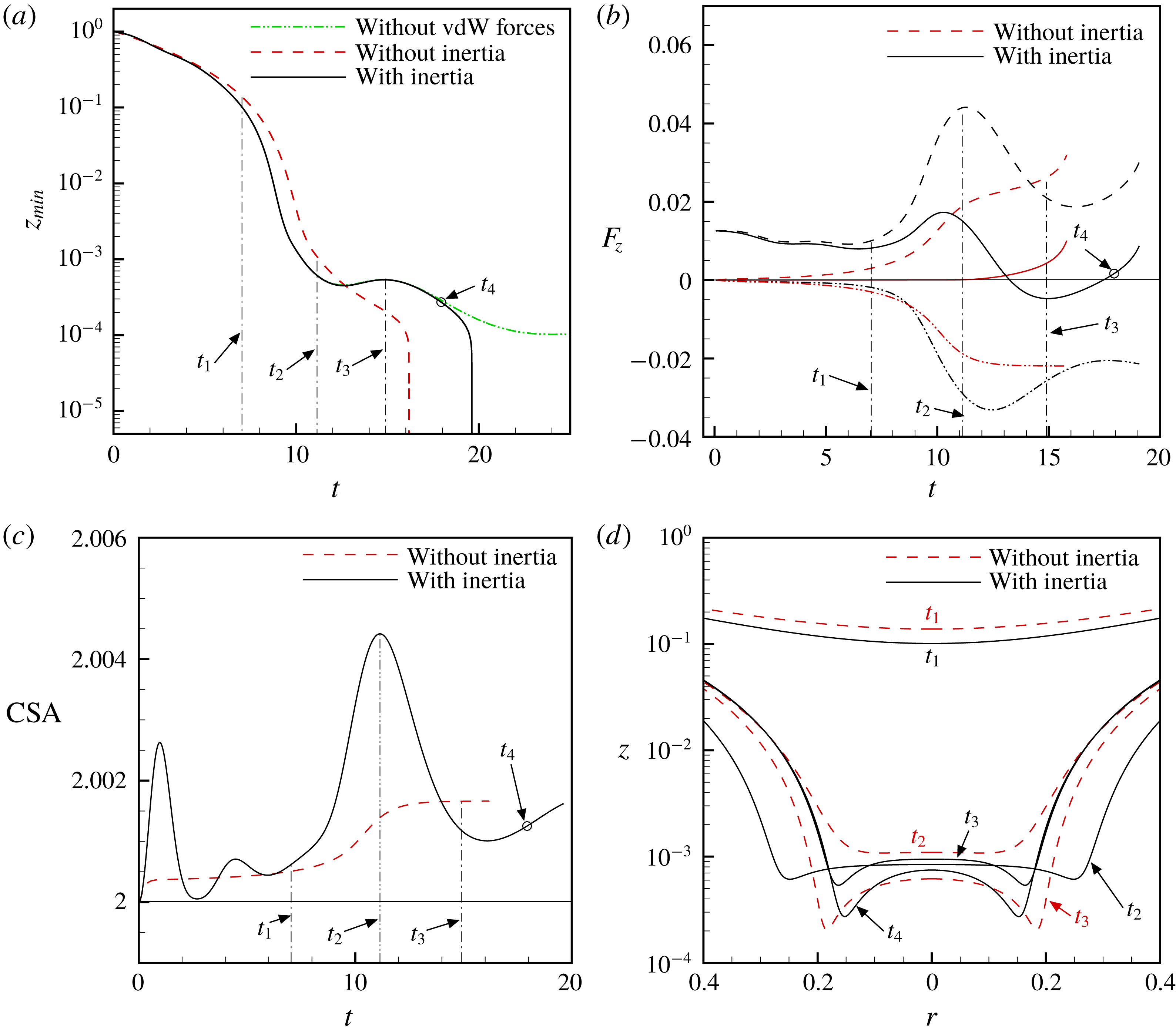
Effects of van der Waals forces and inertia on the evolution in time of the separation between two drops, the net force acting on a drop, the surface area of a drop and drop shapes. For the base case situation identified as ‘With inertia’,
 $Oh=0.02$
,
 $m_{2}=5.26$
,
 $\unicode[STIX]{x1D6FE}_{2}=1.1$
,
 $U_{\infty }=0.095$
and
 $A=4.99\times 10^{-11}$
, and both inertia and van der Waals forces are operative. For the situation identified as ‘Without vdW forces’, all the parameters are the same as in the base case except
 $A=0$
, i.e. the van der Waals force has been turned off. For the situation identified as ‘Without inertia’, all the parameters are the same as in the base case except inertia has been turned off. (a) Evolution in time of half the minimum axial separation between the two drops’ interfaces
 $z_{min}$
for three cases in which both inertia and van der Waals are considered (base case), inertia is considered but van der Waals forces are neglected (Without vdW forces), and when inertia is artificially neglected but van der Waals forces are accounted for (Without inertia). As discussed in the text,
 $t_{1}<t_{2}<t_{3}<t_{4}$
are instances in time when significant events occur during the collision of two drops. (b) Net force
 $F_{z}$
(solid lines), and its components – net force due to pressure
 $F_{z}^{p}$
(dashed lines) and net force due to viscous stress
 $F_{z}^{v}$
(dashed-dotted lines) – in the positive
 $z$
direction determined from (4.1)–(4.3) being exerted by the ambient fluid on the drop when inertia is considered and when inertia is absent. (c) Surface area of the drop when inertia is considered and when inertia is absent. (d) Drop shapes with and without inertia at time instants
 $t_{1}$
,
 $t_{2}$
and
 $t_{3}$
, which are marked by the dashed vertical lines, and at
 $t_{4}$
, which is marked by the open symbol, in (a–c).

Figure 8(a) shows the time evolution of
 $z_{min}$
in the situation in which the dimensionless parameters have the same values as in figure 7 and compares the resulting dynamics to two other situations. In the first of these two other situations, to be discussed in this paragraph, all the dimensionless parameters have the same values as in figure 7 but the van der Waals forces have been ‘turned off’ such that
 $A=0$
. The second of these other situations is discussed in the next paragraph. Comparison of the
 $z_{min}$
versus
 $t$
curves in figure 8(a) for the situation in which van der Waals forces are on (the curve labelled ‘With inertia’ and for which
 $A=4.99\times 10^{-11}$
) and the one for which van der Waals forces have been turned off (the curve labelled ‘Without vdW forces’ and for which
 $A=0$
), it is clear that the forces that eventually cause the film to rupture and the drops to coalesce are the van der Waals forces of attraction or intermolecular forces as the drops do not make contact when these forces are ‘turned off’. As is well known, because the van der Waals forces scale as
 $A/h^{3}$
, they become significant only at very small distances, and cause local rupture of the thin film between the two drops at
 $r_{dimple}$
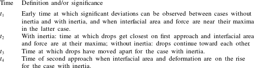
. For the case under investigation, as the two drops approach one another for the first time, they get within a separation of
 $h=2z_{min}\approx 10^{-3}$
at the instant in time
 $t\approx t_{2}$
(instants in time such as
 $t_{2}$
where significant events occur are defined in table 2) when they are closest to each other. It is also clear from figure 8(a) that both curves, viz. the one for which
 $A=4.99\times 10^{-11}$
and the other for which
 $A=0$
, overlap from the initiation of the dynamics until the instant in time corresponding to this value of
 $z_{min}$
and thereby allow one to infer that van der Waals forces are insignificant at this instant, viz.
 $A/h^{3}\ll 1$
, despite the apparent smallness of the gap separating the two drops. However, once the drops rebound but then are driven together by the external flow on their second approach, they get within a minimum separation of the order of
 $h=2z_{min}\approx 4\times 10^{-4}$
at which point the van der Waals forces become significant as
 $A/h^{3}\sim 1$
. Beyond this point in time, which is indicated as the instant
 $t_{4}$
in figure 8(a), the curve corresponding to
 $A\neq 0$
and that corresponding to
 $A=0$
begin to diverge. For the case where van der Waals forces are present, for times
 $t>t_{4}$
their importance continues to grow as the film tends toward rupture and the two drops tend toward contact and coalescence. By contrast, the two drops fail to coalesce when van der Waals forces are absent.
Definitions and/or significance of times
 $t_{1}$
,
 $t_{2}$
,
 $t_{3}$
and
 $t_{4}$
used to identify key instances during the collision and coalescence of two drops.

4.1 Significance of normal force due to pressure in causing rebound
A subtle but inevitable question here is what prevented the drops from getting close enough on their first approach and hence caused them to rebound? Suspecting that the cause is inertia, we test this hypothesis by artificially excluding or throwing out the inertial terms in (2.1b
) and solving a reduced system of equations where the collision of two drops takes place under conditions of Stokes flow. Thus, we compare in this section the coalescence dynamics in two cases: drop coalescence with inertia considered, which is referred hereafter to as ‘with inertia’, and when inertia is ‘turned off’, referred to as ‘without inertia’. Figure 8(a) shows the variation with time of
 $z_{min}$
for these two cases, and it is evident that the presence of inertia alters the mid-stage dynamics of coalescence, e.g. the dynamics in the two cases start deviating from one another as early as
 $t_{1}$
and differ significantly by
 $t_{2}$
. Without inertia, the minimum separation decreases monotonically as a function of time and the drops do not rebound. To gain further insights into the role of inertia, figure 8(b) compares the axial or
 $z$
-component of the net force
 $F_{z}$
exerted by the outer fluid on the top drop, and the contributions to this force that are due to the dynamic pressure
 ${F_{z}}^{p}$
(referred to as the normal force due to pressure) and that due to viscous stress
 ${F_{z}}^{v}$
, in the presence and absence of inertia. These forces are computed as
 $$\begin{eqnarray}\displaystyle & \displaystyle F_{z}=\int _{S}\boldsymbol{n}\boldsymbol{\cdot }\unicode[STIX]{x1D64F}_{2}\boldsymbol{\cdot }\boldsymbol{e}_{z}\,\text{d}S, & \displaystyle\end{eqnarray}$$
 $$\begin{eqnarray}\displaystyle & \displaystyle {F_{z}}^{p}=\int _{S}\boldsymbol{n}\boldsymbol{\cdot }(-p_{2}\boldsymbol{I})\boldsymbol{\cdot }\boldsymbol{e}_{z}\,\text{d}S, & \displaystyle\end{eqnarray}$$
 $$\begin{eqnarray}\displaystyle & \displaystyle {F_{z}}^{v}=\int _{S}\boldsymbol{n}\boldsymbol{\cdot }m_{2}Oh[\unicode[STIX]{x1D735}\boldsymbol{v}_{2}+(\unicode[STIX]{x1D735}\boldsymbol{v}_{2})^{T}]\boldsymbol{\cdot }\boldsymbol{e}_{z}\,\text{d}S. & \displaystyle\end{eqnarray}$$
At time instant
 $t_{1}$
, the drops are separated by
 $z_{min}=10^{-1}$
for the case with inertia, and the pressure in the film region between the drops is rising as the film is draining. Therefore, both
 $F_{z}^{p}$
, shown in figure 8(b), and the drop’s surface area, shown in figure 8(c), are increasing in the instants following
 $t_{1}$
. At this time, the net force
 $F_{z}$
on the drop is positive and increasing, and thus opposing its motion towards the symmetry plane. In contrast, for the case without inertia, while pressure build-up and flattening of the interface also occur in the moments following
 $t_{1}$
, the increases in both
 $F_{z}^{p}$
and the drop’s surface area are much smaller. Furthermore, the increase in
 $F_{z}^{p}$
is balanced by a corresponding decrease in
 $F_{z}^{v}$
, so that the net force
 $F_{z}$
on the drop for the case without inertia is virtually zero. Consequently, the drop in the situation without inertia does not experience any deceleration whatsoever as observed in the situation with inertia.
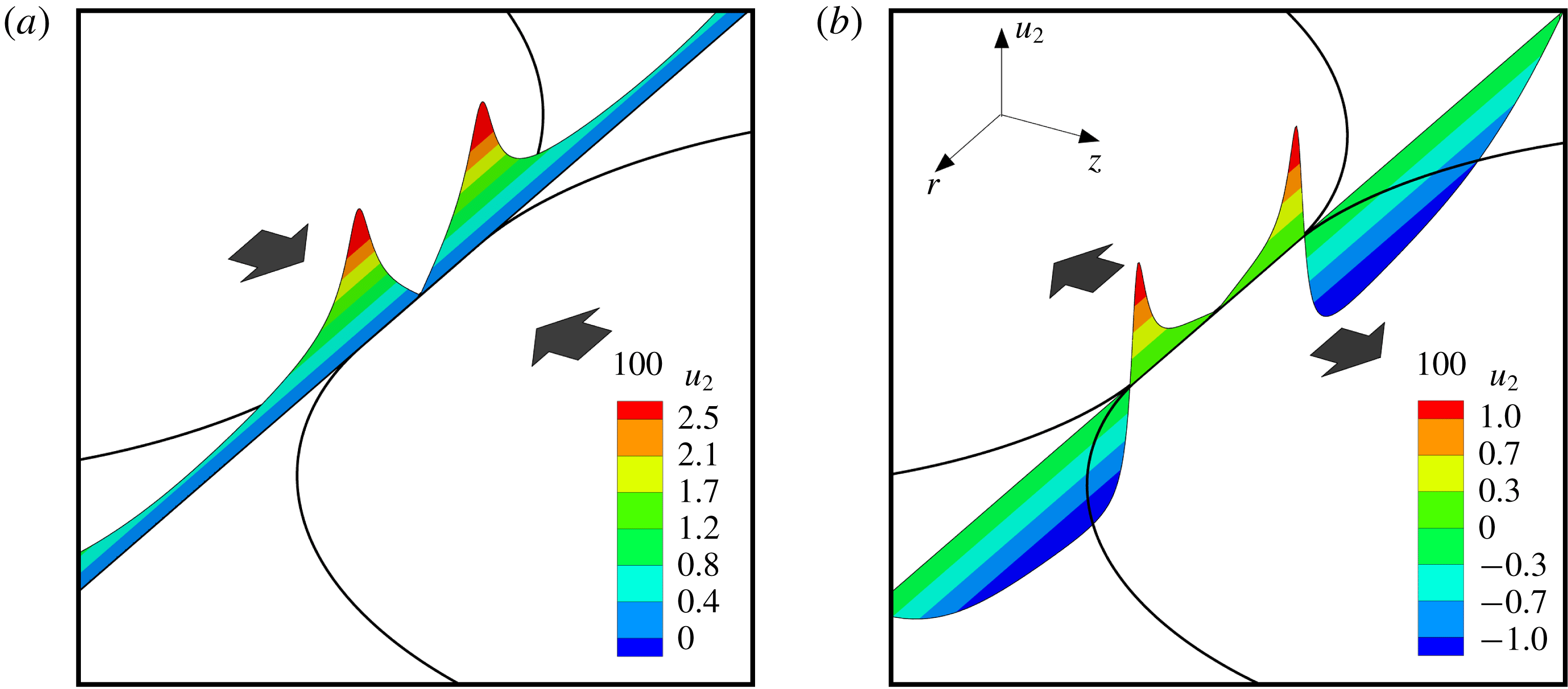
Radial velocity profiles evaluated at the plane of symmetry
 $z=0$
in the film region between two colliding drops at time
 $t=12$
. When inertial effects are turned off, (a), the radial velocity profile is positive everywhere indicating expulsion of the liquid from the region between the drops, i.e. film drainage, and that the drops are continuing to approach each other. However, when inertial effects are included, (b), the radial velocity becomes negative in the region located at the edge of the film. This change in the sign of the radial velocity indicates that fluid is flowing back into the film, thereby opposing film drainage and signalling the onset of drop rebound. Here,
 $Oh=0.02,m_{2}=5.26,\unicode[STIX]{x1D6FE}_{2}=1.1,U_{\infty }=0.095$
and
 $A=4.99\times 10^{-11}$
.

At time
 $t=t_{2}$
, both the force
 $F_{z}^{p}$
and the drop’s surface area for the case with inertia are at their maxima, as a large pressure-induced force acts on the flattened drop. Indeed, the large extent of the interfacial deformation and/or the large value of
 $r_{dimple}$
in this case can both be readily seen in figure 8(d). As the interfaces are separated by
 $z_{min}\approx 10^{-3}$
at this instant, van der Waals forces are unable to cause rupture of the film, and because of the large positive value of
 $F_{z}$
the drops are pushed away from each other, thereby causing the outer liquid to flow back into the film region (see below). In the moments following
 $t_{2}$
, the drop with inertia tends towards its spherical shape as the pressure-induced force decreases. In contrast, the dynamics is remarkably different over this period in time for the case without inertia as the magnitude of
 $F_{z}^{p}$
acting on the drop is much smaller, and consequently the extent of the deformation of the interface is much smaller compared to the case with inertia. As the net force
 $F_{z}$
is still virtually zero in this case, the drops continue to approach each other. Another key contrast between the two cases can be gleaned from the simulation results by examination of the radial velocity profiles in the film at time
 $t=12$
such that
 $t_{2}<t=12<t_{3}$
(see figure 9). For the case without inertia, the radial velocity
 $u_{2}$
is positive everywhere in the film including its edges (figure 9
a), indicating that fluid is being expelled from the film region and that the drops are continuing to approach each other. Thus, in the case without inertia, the interfaces are able to get close enough to one another for van der Waals attraction to become significant and for the drops to coalesce without any rebound effects. However, for the case with inertia (figure 9
b), the radial velocity is negative in the vicinity of the film’s edges, indicating that fluid is flowing into the film and that the drops are moving away from each other.
When
 $t\approx t_{3}$
, the drops in the case with inertia have moved apart and the value of
 $r_{dimple}$
has fallen to a small value. Viscous force
 $F_{z}^{v}$
, which had heretofore been sub-dominant, has now become dominant and results in a net negative
 $F_{z}$
that pushes the drops back towards each other. This causes the interfaces of the two drops to deform and the interfacial area to increase for the second time. For the case without inertia, pressure in the film is large enough to dominate viscous stress, and the resulting net positive
 $F_{z}$
begins to cause the drops to slow down. However, as the separation falls to
 $z_{min}\approx 2\times 10^{-4}$
, van der Waals forces of attraction become significant. Thus, in the moments following
 $t_{3}$
, rapid local thinning of the film separating the drops occurs at the radial location of
 $r_{dimple}$
for the case without inertia and the separation between the two drops quickly reaches molecular length scales, signalling the incipience of drop coalescence. For the case with inertia, both interface deformation and interfacial area continue to increase as the drops continue to approach each other for times
 $t\approx t_{4}$
. However, the deformation of the drop is much smaller during this second approach compared to that on the first approach as the pressure-induced force opposing the approach is much lower compared to that during the first approach. On this second approach, the drops are able to get sufficiently close so that by the time
 $z_{min}\approx 2\times 10^{-4}$
the van der Waals forces have become large enough to initiate the intermolecular force-driven rupture of the film separating the drops. Thus, in summary, for coalescence at
 $Re=1$
, inertial effects lead to a net positive
 $F_{z}$
acting on the drop during the mid to the late stages of coalescence, resulting in a much larger deformation or
 $r_{dimple}$
in comparison to the ‘Stokes’ case, causing the drops to decelerate and eventually to rebound. Consequently, it is on the subsequent approach that the drops are able to get sufficiently close for van der Waals forces to become large enough to rupture the thin film and lead to coalescence.
4.2 Pressure build-up in the film due to inertia
A natural question that arises from the results presented in the previous subsection is why the normal force
 $F_{z}^{p}$
due to pressure is much larger when inertia is present in comparison to when inertia is neglected during the initial approach of the two drops (starting at
 $t\approx 8$
in figure 8). We turn to an analysis of the governing equations for the liquid velocities and pressure in the film along the plane of symmetry
 $z=0$
to provide the required insights. The continuity equation in the film of outer liquid can be written as
 $$\begin{eqnarray}\frac{1}{r}\frac{\unicode[STIX]{x2202}}{\unicode[STIX]{x2202}r}(ru_{2})=-\frac{\unicode[STIX]{x2202}w_{2}}{\unicode[STIX]{x2202}z}.\end{eqnarray}$$
In both drop coalescence and the dynamics of thin free films, or liquid sheets, the gradient of
 $u_{2}$
in the axial direction is small compared to its gradient in the radial direction, or
 $\unicode[STIX]{x2202}u_{2}/\unicode[STIX]{x2202}z\ll \unicode[STIX]{x2202}u_{2}/\unicode[STIX]{x2202}r$
. Thus, the
 $r$
-component of the Navier–Stokes equation (2.1b
) in the film of outer liquid reduces to
 $$\begin{eqnarray}\unicode[STIX]{x1D6FE}_{2}\left(\frac{\unicode[STIX]{x2202}u_{2}}{\unicode[STIX]{x2202}t}+u_{2}\frac{\unicode[STIX]{x2202}u_{2}}{\unicode[STIX]{x2202}r}\right)=-\frac{\unicode[STIX]{x2202}p_{2}}{\unicode[STIX]{x2202}r}+m_{2}Oh\frac{\unicode[STIX]{x2202}}{\unicode[STIX]{x2202}r}\left(\frac{1}{r}\frac{\unicode[STIX]{x2202}}{\unicode[STIX]{x2202}r}(ru_{2})\right).\end{eqnarray}$$
Substituting (4.4) into (4.5) gives
 $$\begin{eqnarray}\unicode[STIX]{x1D6FE}_{2}\left(\frac{\unicode[STIX]{x2202}u_{2}}{\unicode[STIX]{x2202}t}+u_{2}\frac{\unicode[STIX]{x2202}u_{2}}{\unicode[STIX]{x2202}r}\right)=-\frac{\unicode[STIX]{x2202}p_{2}}{\unicode[STIX]{x2202}r}-m_{2}Oh\frac{\unicode[STIX]{x2202}}{\unicode[STIX]{x2202}r}\left(\frac{\unicode[STIX]{x2202}w_{2}}{\unicode[STIX]{x2202}z}\right).\end{eqnarray}$$
At the symmetry plane
 $z=0$
,
 $w_{2}=0$
and thus the
 $z$
-component of the Navier–Stokes equation (2.1b
) is given by
 $$\begin{eqnarray}0=-\frac{\unicode[STIX]{x2202}p_{2}}{\unicode[STIX]{x2202}z}+m_{2}Oh\frac{\unicode[STIX]{x2202}^{2}w_{2}}{\unicode[STIX]{x2202}z^{2}}.\end{eqnarray}$$
The last equation reduces to
 $\unicode[STIX]{x2202}p_{2}/\unicode[STIX]{x2202}z=0$
from the continuity equation and the earlier assumption of the smallness of the axial gradient of
 $u_{2}$
. Thus, equation (4.6) can be integrated with respect to
 $r$
from
 $r=0$
to
 $r=r_{e}$
, where
 $r_{e}$
is a radial location just outside the film region such that the pressure in the outer fluid is equal to the datum pressure, to give
 $$\begin{eqnarray}\int _{0}^{r_{e}}\unicode[STIX]{x1D6FE}_{2}\left(\frac{\unicode[STIX]{x2202}u_{2}}{\unicode[STIX]{x2202}t}+u_{2}\frac{\unicode[STIX]{x2202}u_{2}}{\unicode[STIX]{x2202}r}\right)\,\text{d}r=-p_{2}|_{r_{e}}+p_{2}|_{r=0}-m_{2}Oh\left[\left(\frac{\unicode[STIX]{x2202}w_{2}}{\unicode[STIX]{x2202}z}\right)_{r_{e}}-\left(\frac{\unicode[STIX]{x2202}w_{2}}{\unicode[STIX]{x2202}z}\right)_{0}\right].\end{eqnarray}$$
Therefore, the pressure in the film at the axis of symmetry
 $r=0$
, denoted by
 $p_{0}$
, is then given by
 $$\begin{eqnarray}\displaystyle p_{0}=p_{2}|_{r_{e}}+\underbrace{m_{2}Oh\left[\left(\frac{\unicode[STIX]{x2202}w_{2}}{\unicode[STIX]{x2202}z}\right)_{r_{e}}-\left(\frac{\unicode[STIX]{x2202}w_{2}}{\unicode[STIX]{x2202}z}\right)_{0}\right]}_{V}+\underbrace{\int _{0}^{r_{e}}\unicode[STIX]{x1D6FE}_{2}\left(\frac{\unicode[STIX]{x2202}u_{2}}{\unicode[STIX]{x2202}t}+u_{2}\frac{\unicode[STIX]{x2202}u_{2}}{\unicode[STIX]{x2202}r}\right)\,\text{d}r}_{I}, & & \displaystyle\end{eqnarray}$$
where
 $V$
stands for the viscous term and
 $I$
the inertial term. If the scale of the axial velocity and that of the axial distance are estimated by the centre-of-mass velocity of the drop
 $v_{com}$
and the local film thickness
 $h$
,
 $\unicode[STIX]{x2202}w_{2}/\unicode[STIX]{x2202}z\sim v_{com}/h$
, then the pressure at the centre of the film is given by
 $$\begin{eqnarray}\displaystyle p_{0}\approx p_{2}|_{r_{e}}+\underbrace{m_{2}\,Oh\,v_{com}\left[\left(\frac{1}{h}\right)_{r_{e}}-\left(\frac{1}{h}\right)_{r=0}\right]}_{V}+\underbrace{\int _{0}^{r_{e}}\unicode[STIX]{x1D6FE}_{2}\left(\frac{\unicode[STIX]{x2202}u_{2}}{\unicode[STIX]{x2202}t}+u_{2}\frac{\unicode[STIX]{x2202}u_{2}}{\unicode[STIX]{x2202}r}\right)\,\text{d}r}_{I}. & & \displaystyle\end{eqnarray}$$
The viscous term (
 $V$
) is positive as the film thickness is such that
 $h_{r_{e}}>h_{r=0}$
while
 $v_{com}$
is negative. Moreover, the inertial term (
 $I$
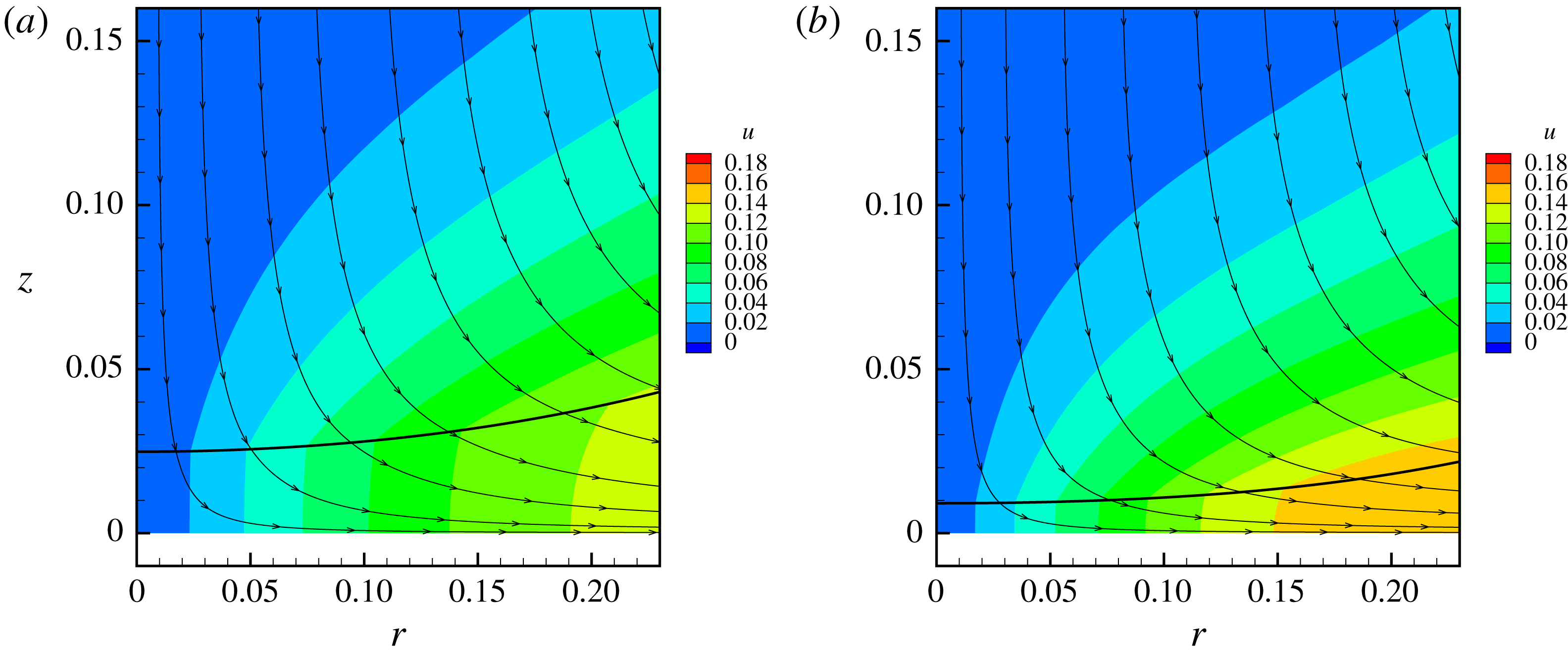
) is positive because as the drop approaches the plane of symmetry, the radial velocity, which is non-negative, increases both in time and in the radial direction. The correctness of the last assertion is verified by interrogation of the radial velocity field determined from simulations, as highlighted by the contour plots shown in figure 10. In contrast, if inertia is excluded from the governing equations, the pressure in the film at the axis
 $p_{0}^{stokes}$
is now given by
 $$\begin{eqnarray}\displaystyle p_{0}^{stokes}\approx p_{2}|_{r_{e}}+\underbrace{m_{2}Ohv_{com}\left[\left(\frac{1}{h}\right)_{r_{e}}-\left(\frac{1}{h}\right)_{r=0}\right]}_{V}. & & \displaystyle\end{eqnarray}$$
In other words, because of the presence of the additional positive inertial term (
 $I$
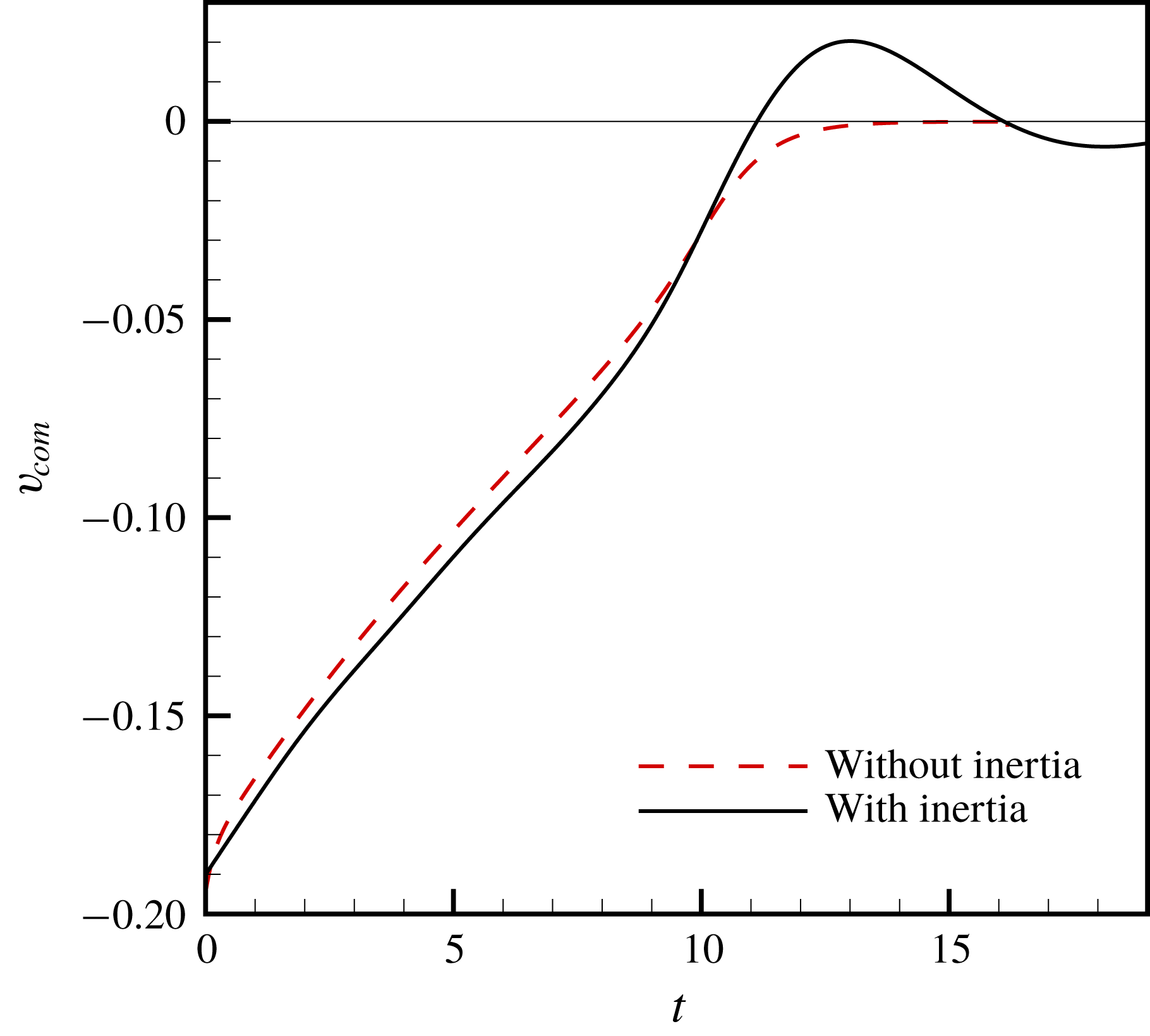
) in the case with inertia compared to that in the absence of inertia, the pressure in the film is larger when inertia is included than when it is neglected during the initial stages of the approach of the two drops. Additionally, figure 11 shows the variation of the velocity of the centre of mass
 $v_{com}$
of the top drop with time for the two cases. This figure makes plain that the magnitude of
 $v_{com}$
is larger in the case with inertia than without until
 $t\approx 8$
after which the net positive
 $F_{z}$
acting on the drop begins to cause it to decelerate in the case with inertia. Thus, the viscous term (
 $V$
) is also larger until this time when inertia is considered compared to when it is not. In conclusion,
 $p_{0}>p_{0}^{stokes}$
during virtually the entire time that the two drops are approaching one another in the case with inertia. Thus, when inertia is considered, the larger pressure in the film causes the larger normal force on the drop, which in turn leads to the rebound dynamics as explained in § 4.1.
Contours of the radial velocity
 $u$
at two instants in time, (a)
 $t=8.31$
and (b)
 $t=8.79$
, in the thin film that forms between the colliding drops. The liquid–liquid interface is shown by the solid black line. Here, the values of the parameters are identical to those in figure 8. The radial velocity is positive and increases both in time
 $t$
and radial direction
 $r$
.

The variation with time of the velocity of the centre of mass
 $v_{com}$
of the drop in two cases: (i) when inertia is considered and (ii) when inertia is neglected from the governing equations. The horizontal line represents
 $v_{com}=0$
and helps to highlight the bounce experienced by the drop when inertia is considered. Here, the values of the parameters are identical to those in figure 8.

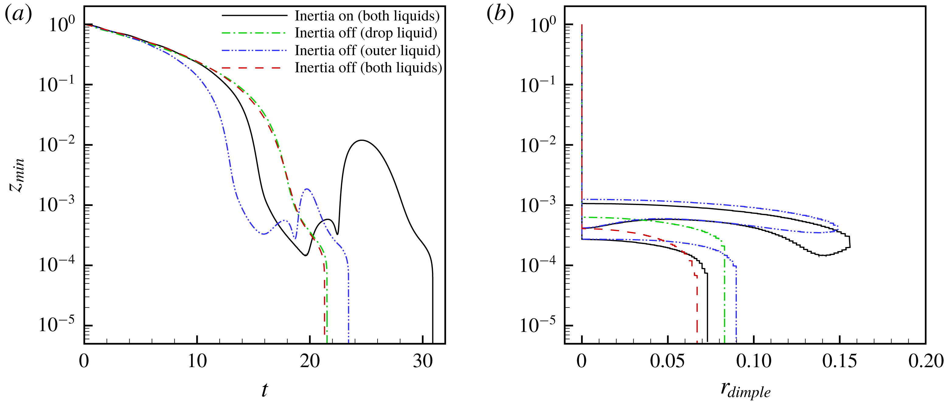
(a) Variation in time of half the minimum separation
 $z_{min}$
between two drops in four cases: (i) inertial effects are considered for both liquids, (ii) inertial effects are turned off for the drop liquid, (iii) inertial effects are turned off for the outer liquid and (iv) inertial effects are neglected for both liquids (Stokes flow). (b) Variation of
 $z_{min}$
with the radius of the dimple
 $r_{dimple}$
that forms during mid to late stages of coalescence to highlight the extent of drop deformation in the four cases. Here,
 $Oh=0.023,m_{2}=1,\unicode[STIX]{x1D6FE}_{2}=1,U_{\infty }=0.05$
and
 $A=10^{-10}$
. Thus,
 $Ca=0.0015$
in all four cases.

4.3 The significance of drop or dispersed phase inertia
We next examine the role each phase’s inertia plays in drop rebound. Figure 12(a) shows the variation with time of
 $z_{min}$
for two liquid drops that are driven to collision in a second immiscible liquid of identical viscosity and density (
 $Oh=0.023$
,
 $m_{2}=1$
,
 $\unicode[STIX]{x1D6FE}_{2}=1$
,
 $U_{\infty }=0.05$
and
 $A=10^{-10}$
) in four cases: (i) inertial effects are considered for both liquids, (ii) inertial effects are excluded from the momentum equations for the drop liquid, (iii) inertial effects are excluded from the momentum equations for the outer liquid and (iv) inertial effects are excluded from the momentum equations for both liquids so that both phases are undergoing Stokes flow.
For case i, the drops approach each other until half the minimum separation has fallen to
 $z_{min}\approx 2.0\times 10^{-4}$
after which the drops rebound. After rebounding, the interfaces locally approach each other again, before separating by a much larger distance than after the first rebound. The drops finally coalesce after the two interfaces approach each other for the third time (figure 12
a).
At the other end of the spectrum, for case iv where both liquids are undergoing Stokes flow,
 $z_{min}$
decreases monotonically with time and without any rebound (figure 12
a). Consequently, the drainage time for case iv is much smaller than that for case i.
However, when inertial effects are only turned off for the drop liquid, case ii, the variation of
 $z_{min}$
with time is identical to that observed when both liquids are undergoing Stokes flow (case iv discussed in the previous paragraph), as shown in figure 12(a). By contrast, excluding inertial effects in the outer liquid alone, case iii, has a much more modest impact on the dynamics. For case iii, similar to case i, the drops are observed to rebound upon first approach, and coalesce on the third approach of the interfaces towards each other (figure 12
a). The magnitude of the rebound, however, is suppressed in case iii compared to case i, with the accompanying result that the drainage time in case iii is smaller than that in case i. Indeed, the absence of inertia in the outer liquid in case iii ensures that the viscous force (
 $F_{z}^{v}$
from 4.3) dominates and pushes the drops back together more rapidly as compared to case i.
Figure 12(b) shows the variation of
 $z_{min}$
with the extent of drop deformation that is characterized by
 $r_{dimple}$
in the aforementioned four cases. Dimple formation, and the consequent slowdown of film drainage, begins at a separation of
 $z_{min}\sim 10^{-3}$
where
 $A/h^{3}\ll 1$
for cases i and iii where inertia is included in either both phases or the dispersed phase. Thus, attractive van der Waals forces are negligible while the opposing hydrodynamic force is large at this stage of drop collision in both cases, resulting in the observed rebound. In contrast, for cases ii and iv where inertia is excluded from either the dispersed phase or both phases and where no rebound is observed, dimple formation begins at a much lower value of the separation between the drops: it commences when
 $z_{min}\approx 5\times 10^{-4}$
, where
 $A/h^{-3}\sim O(1)$
, and hence attractive van der Waals forces are large enough to drive the drops to coalesce on their first approach. In conclusion, it is clear from the results of figure 12 that inertia of the drop liquid, as opposed to inertia of the outer liquid, is primarily responsible for rebound. Moreover, the inclusion of inertia of the drop liquid results in early dimple formation and subsequent slowdown of film drainage, much before van der Waals forces are significant enough to cause local film rupture.
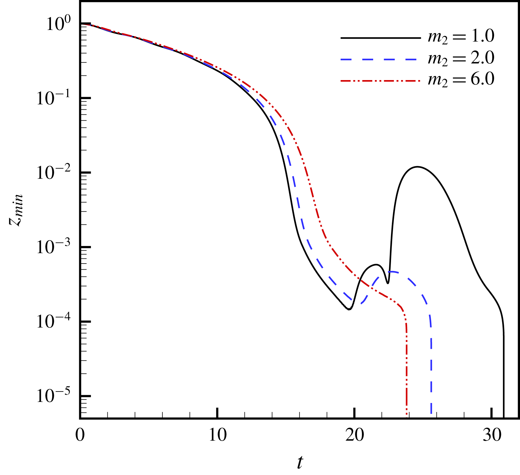
Effect of the viscosity ratio
 $m_{2}$
on drop rebound and drainage time
 $t_{d}$
: the variation of half the minimum separation
 $z_{min}$
with time
 $t$
. For the three cases shown, the ratio of the viscosity of the outer fluid to the drop fluid is varied from one to six as indicated in the legend while all the other dimensionless groups are held fixed. The computed values of the drainage time are:
 $t_{d}=16.06$
when
 $m_{2}=1$
and the drops rebound twice,
 $t_{d}=10.51$
when
 $m_{2}=2$
and there is one rebound and
 $t_{d}=8.33$
when
 $m_{2}=6$
and there is no rebound. Here,
 $Oh=0.023,\unicode[STIX]{x1D6FE}_{2}=1,U_{\infty }=0.05$
and
 $A=10^{-10}$
.

4.4 The impact of drop rebound on drainage times
An important consequence of drop rebound that arises when two drops are undergoing collision and coalescence in situations in which inertia is important is the increase in film drainage time
 $t_{d}$
(cf. § 1). This time scale is a key parameter in population balance models that are widely used in engineering design of certain types equipment and devices such as coalescers, desalters and dehydrators which are common, among others, in the oil and gas industry (Bajpai et al.
Reference Bajpai, Ramkrishna and Prokop1976; Tobin et al.
Reference Tobin, Muralidhar, Wright and Ramkrishna1990; Zhang et al.
Reference Zhang, Basaran and Wham1995). Figure 13 shows the variation with time of
 $z_{min}$
for two liquid drops that are driven to collision in a second immiscible liquid of identical density in three situations in which the viscosity ratio
 $m_{2}$
is increased from
 $m_{2}=1$
to
 $m_{2}=6$
. When the outer liquid is of comparable viscosity to the inner liquid or
 $m_{2}=1$
, the drops rebound twice before coalescing on the third approach. In this case, coalescence is delayed because of the number of rebounds and the computed value of the drainage time,
 $t_{d}=16.06$
, is large. However, as the viscosity of the outer fluid is systematically increased to
 $m_{2}=6$
, the number of drop rebounds decreases from two to zero, and the value of the drainage time is nearly halved, as shown in the figure. In previous works, researchers (Janssen et al.
Reference Janssen, Anderson, Peters and Meijer2006; Yoon et al.
Reference Yoon, Baldessari, Ceniceros and Leal2007) have developed scaling laws for the drainage time as a function of capillary number,
 $\tilde{t}_{d}G\sim Ca^{m}$
. The value of the scaling exponent
 $m$
has been reported to equal
 $3/2$
by Chesters (Reference Chesters1991), Yang et al. (Reference Yang, Park, Hu and Leal2001) and Janssen et al. (Reference Janssen, Anderson, Peters and Meijer2006), and was later updated to be
 $4/3$
by Yoon et al. (Reference Yoon, Baldessari, Ceniceros and Leal2007) and Frostad et al. (Reference Frostad, Walter and Leal2013). While the value of the scaling exponent is not yet universally agreed upon (Janssen & Anderson Reference Janssen and Anderson2011), it is clear from figure 13 that the effect of inertia on drainage time adds a new and important dimension to this ongoing debate.
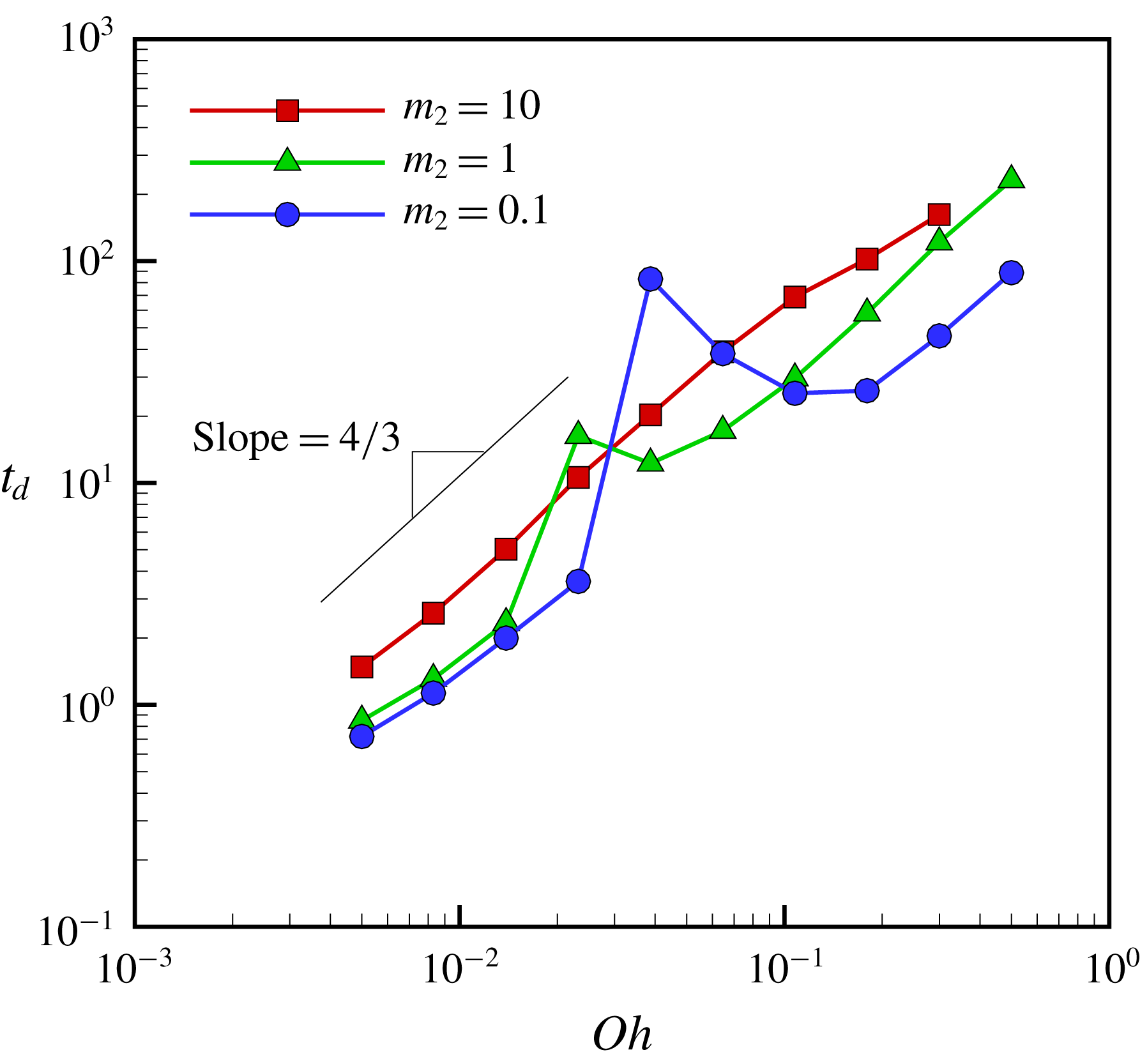
Variation of drainage time
 $t_{d}$
with Ohnesorge number
 $Oh$
for three different values of the viscosity ratio
 $m_{2}$
while holding fixed the remaining dimensionless groups at
 $\unicode[STIX]{x1D6FE}_{2}=1,U_{\infty }=0.05$
and
 $A=10^{-10}$
. The short straight line of slope
 $4/3$
helps indicate that with the exception of parameter values where
 $t_{d}$
exhibits a spike as discussed in the body of the text, the simulation results follow the
 $4/3$
scaling law deduced in previous studies of coalescence (Yoon et al.
Reference Yoon, Baldessari, Ceniceros and Leal2007).

Figure 14 shows the variation of the drainage time
 $t_{d}$
with Ohnesorge number
 $Oh$
for three different values of
 $m_{2}$
, holding all other parameters fixed at
 $\unicode[STIX]{x1D6FE}_{2}=1,U_{\infty }=0.05$
and
 $A=10^{-10}$
. These results show that for situations in which
 $m_{2}=10$
, the response is quite similar to that which occurs in Stokes flow: drainage time monotonically increases with
 $Oh$
with a scaling exponent of
 $4/3$
. As
 $m_{2}$
,
 $G$
and
 $U_{\infty }$
are held constant, we can infer from (2.4) that
 $\tilde{t}_{d}G\sim Ca^{4/3}$
in this case, in accord with the results of Yoon et al. (Reference Yoon, Baldessari, Ceniceros and Leal2007). However, when the external liquid is of comparable or lower viscosity than the drop liquid (
 $m_{2}=1$
or 0.1), drainage time does not vary monotonically with
 $Oh$
. Indeed, there is a jump or a spike at intermediate values of
 $Oh$
in the curves depicting drainage time versus Ohnesorge number and a clear departure of computed results from the expected scaling law.
(a) Time variation of
 $z_{min}$
for low, intermediate and high values of
 $Oh$
corresponding to before, at and after the ‘spike’ in figure 14 (
 $m_{2}=1,\unicode[STIX]{x1D6FE}_{2}=1,U_{\infty }=0.05$
and
 $A=10^{-10}$
). The drop trajectories reveal that the increase in drainage time and hence the ‘spike’ is because the drops of intermediate values of
 $Oh$
do not coalesce on first approach, rebound, and finally do coalesce on the second approach. (b) Time variation of
 $z_{min}$
for more viscous systems (higher
 $Oh$
values of
 $0.108<Oh<0.5$
) showing no rebound effect and that the drops coalesce on first approach. (c) Time variation of
 $z_{min}$
for a less viscous or a more highly inertial system (
 $Oh=0.005$
) shows that the drops coalesce on first approach. However, if the van der Waals forces are artificially turned off when
 $Oh=0.005$
, the drops bounce to a further extent than when the Ohnesorge number is larger (
 $Oh=0.023$
) but the van der Waals forces are on.

Interrogation of simulation results to examine the drop trajectories for situations in which the spikes and hence the departure from the usual scaling law occur reveals that the deviation from the
 $4/3$
scaling theory for drainage time is due to the inertia-driven rebound of drops. Figure 15(a) shows the time evolution of
 $z_{min}$
for drop pairs where
 $Oh=0.008,0.023$
and 0.065. While drainage times for
 $Oh=0.008$
and
 $Oh=0.065$
conform to the
 $4/3$
scaling law and where
 $z_{min}$
decreases monotonically with time, the drainage time for
 $Oh=0.023$
departs from the
 $4/3$
scaling law and a clear rebound effect is observed in the computed evolution of
 $z_{min}$
with time. It accords with intuition that for larger values of
 $Oh$
, the system is more viscous and inertial effects should therefore be less pronounced. Hence, there is no rebound phenomenon, as shown in figure 15(b), when the value of
 $Oh$
is sufficiently large. Intuition further dictates that for smaller values of
 $Oh$
, inertial effects should be more pronounced and drop rebound should occur. However, for even smaller values of
 $Oh$
, unexpectedly the drops coalesce before rebounding. This apparent contradiction is resolved by realizing that when viscous resistance to flow and hence drainage of the film separating two drops is lower, the drops are able to get closer to one another on the first approach. Thus, when this distance on first approach is sufficiently small for van der Waals forces to become important, the film is able to rupture rapidly before pressure in the film can rise and oppose the approach of the drops toward each other. The correctness of this surmise can be readily verified by artificially turning off the van der Waals forces at extremely low values of
 $Oh$
(e.g.
 $Oh=0.005$
). As shown in figure 15(c), whereas two low-viscosity drops of
 $Oh=0.005$
rapidly coalesce, two drops of the same
 $Oh$
but with van der Waals forces turned off (
 $Oh=0.005$
, (vdW terms turned off)) bounce back to a greater extent than two drops of slightly higher viscosity of
 $Oh=0.023$
.
5 Conclusions
The approach, collision and coalescence dynamics of two drops suspended in a second liquid where both fluids are incompressible, Newtonian fluids of constant physical properties have been studied using a multi-scale, method of lines, arbitrary Lagrangian–Eulerian algorithm that utilizes the Galerkin finite element method and elliptic mesh generation for spatial discretization and adaptive finite differences for time integration. The multi-scale nature of the problem is dictated by the fact that whereas the two drops initially each have a dimensionless radius of one and centre-to-centre separation equal to some order-one multiple of their radii, the thickness of the film of the exterior liquid that separates the approaching drops has to fall by roughly five orders of magnitude before film rupture and hence coalescence can be said to have occurred (for example, if the radii of the undisturbed drops are 1 mm, a dimensional film thickness of 10 nm or a dimensionless film thickness of
 $10^{-5}$
has to be reached before coalescence is said to have occurred). Here, accurate resolution of the dynamics occurring over such disparate length scales has been made possible by use of the aforementioned sharp interface algorithm (Castrejón-Pita et al.
Reference Castrejón-Pita, Castrejón-Pita, Thete, Sambath, Hutchings, Hinch, Lister and Basaran2015) (see also Li & Sprittles (Reference Li and Sprittles2016) who have used algorithms that are similar to ours). Variants of the algorithm employed in this paper have already been used successfully to resolve pinch-off (Suryo & Basaran Reference Suryo and Basaran2006; Castrejón-Pita et al.
Reference Castrejón-Pita, Castrejón-Pita, Thete, Sambath, Hutchings, Hinch, Lister and Basaran2015; Kamat et al.
Reference Kamat, Wagoner, Thete and Basaran2018), film rupture (Garg et al.
Reference Garg, Kamat, Anthony, Thete and Basaran2017) and post-coalescence (Munro et al.
Reference Munro, Anthony, Basaran and Lister2015; Anthony Reference Anthony2017) dynamics involving drops, films and bubbles where length scales that differ by 4–6 orders of magnitude are commonly encountered, and the most advanced versions of which can achieve yet bigger disparities in length scales of the order of
 $10^{7}$
or larger (Anthony & Basaran Reference Anthony and Basaran2018, Reference Anthony and Basaran2019). According to the results of the foregoing analysis, inertia plays a key role in delaying drop coalescence by causing two colliding drops to rebound one or more times before finally coalescing. Also according to the foregoing analysis, whereas inertia of the drop fluid is crucial to giving rise to rebound effects, its absence results in coalescence dynamics that is similar to that observed in Stokes flow. Plainly, existing scaling theories for film drainage and coalescence times need to be revisited and carefully revised when inertial effects are important.
A situation that is related to that studied in the present paper arises in applications such as sprays and combustion where two drops collide in a gas (Qian & Law Reference Qian and Law1997) or when a drop falls through a gas onto a bath of the same liquid as the drop (Couder et al. Reference Couder, Fort, Gautier and Boudaoud2005; Geri et al. Reference Geri, Keshavarz, McKinley and Bush2017). In these problems also, the thin lubricating air layer between the two drops or the drop and the bath must drain to a critical thickness before coalescence is initiated by intermolecular forces. Moreover, as in this work, the collision between the two liquid surfaces can lead to a rebound (Rayleigh Reference Rayleigh1899; Qian & Law Reference Qian and Law1997). In fact, a drop colliding with a liquid bath can be prevented from coalescing and be made to undergo oscillatory bouncing or rebounding for an arbitrarily long time by vertically vibrating the bath (Walker Reference Walker1978; Couder et al. Reference Couder, Fort, Gautier and Boudaoud2005). A distinguishing feature of studies where a drop may repeatedly bounce on a liquid surface is that the viscosity ratio between the inner (drop) and the outer (gas) fluids in such studies is between five thousand and a million whereas it is between 0.1 and 10 in the present paper. Moreover, whereas the two fluids in our paper are of nearly equal densities, the density contrast in these other studies is about 1000. Therefore, viscous dissipation in the films separating the two drops in our paper is much larger than that in these other studies. This difference makes the phenomenon of drop bouncing all the more remarkable and unexpected in our case compared to the other studies where the surrounding fluid is a gas.
The results presented in this paper can be extended in a number of other fruitful directions as summarized in this and the following paragraphs. As discussed earlier in the paper, the dynamics of coalescence is governed by five dimensionless groups when the drops have the same radii. For most liquid–liquid systems, the density ratio
 $\unicode[STIX]{x1D6FE}_{2}$
is approximately equal to one. Therefore, it would be highly desirable to conduct a comprehensive study in the future to determine the effect of the Ohnesorge number
 $Oh$
, the viscosity ratio
 $m_{2}$
, the dimensionless approach velocity
 $U_{\infty }$
and the ratio of the radii of the two drops
 $R_{1}/R_{2}$
even in situations in which the drops have the same densities and the van der Waals number
 $A$
is held fixed on the coalescence dynamics, paying particular attention to drop rebound and its effect on scaling theories for drainage times. The dependence of drainage times on both approach velocity and ratio of drop radii will be especially significant in industrial coalescers with agitators where large spatial variations in flow and drop sizes can occur (Bajpai et al.
Reference Bajpai, Ramkrishna and Prokop1976).
The drainage and coalescence dynamics can be significantly altered by the presence of surfactants and/or surface-active chemicals. Many industrial applications involve emulsions containing emulsifying agents and contaminants. It has been shown experimentally (Hu, Pine & Leal Reference Hu, Pine and Leal2000) and computationally (Chesters & Bazhlekov Reference Chesters and Bazhlekov2000; Dai & Leal Reference Dai and Leal2008; Vannozzi Reference Vannozzi2012) that under Stokes flow conditions, film drainage slows down significantly in the presence of surfactants and that coalescence may even be altogether inhibited. However, many industrial applications involve systems where the fluids are not undergoing Stokes flow and where inertia cannot be neglected.
A very popular and successful technique to destabilize emulsions in applications involves the use of electric fields which greatly increases the chance of drops approaching each other and ultimately coalescing (Zhang et al. Reference Zhang, Basaran and Wham1995). Moreover, electric fields have also been deployed in quantifying the stability of emulsions. Among other things, recent experiments of Ristenpart et al. (Reference Ristenpart, Bird, Belmonte, Dollar and Stone2009) have shown that contrary to conventional wisdom, oppositely charged drops may not necessarily coalesce when brought together. Clearly, thorough and careful computational analyses of drop coalescence under an applied electric field will go a long way toward improving the existing understanding of the underlying dynamics and broadly impact the usefulness and efficiency of electrically enhanced coalescers and separators that are widely used in the oil, gas and chemical industries (Ptasinski & Kerkhof Reference Ptasinski and Kerkhof1992; Eow & Ghadiri Reference Eow and Ghadiri2002). The numerical methods utilized by Collins et al. (Reference Collins, Jones, Harris and Basaran2008) and Collins et al. (Reference Collins, Sambath, Harris and Basaran2013) for studying electrohydrodynamic tip streaming from liquid drops and films can be combined with the methods used in this paper to rigorously model the electrocoalescence of drops. We plan to report the results of such studies in the future.
In certain situations, the drops can collide off centre and the dynamics will not be axisymmetric as in this paper. A number of researchers have already addressed off-centre or asymmetric collisions where the flow is fully three-dimensional but all such studies where the dynamics of the thin film separating the two drops has been well resolved pertain to situations where inertia is negligible and the dynamics can be described by the creeping flow equations rather than the nonlinear Navier–Stokes equations solved in this paper (Rother et al. Reference Rother, Zinchenko and Davis1997; Zinchenko et al. Reference Zinchenko, Rother and Davis1997; Rother & Davis Reference Rother and Davis2001). The approach based on the Galerkin finite element method used to analyse axisymmetric flows in this paper has been extended to fully three-dimensional flows with inertia (Baer et al. Reference Baer, Cairncross, Schunk, Rao and Sackinger2000; Cairncross et al. Reference Cairncross, Schunk, Baer, Rao and Sackinger2000) and, in very recent work, Tsamopoulos and coworkers (Fraggedakis et al. Reference Fraggedakis, Papaioannou, Dimakopoulos and Tsamopoulos2017) have implemented the elliptic mesh generation algorithm that has been successfully used in this paper to solve three-dimensional free surface flows. Despite their promise, it has not been demonstrated in these recent papers that disparities in length scales that arise during studies of drop coalescence can be resolved by these three-dimensional algorithms. Therefore, another goal of future work will be to analyse the fluid mechanics of off-axis collisions and its effect on coalescence and/or drainage times by appropriately combining certain features of the multi-scale algorithm used in this paper with advances reported in these recent publications.
Acknowledgements
This work was supported by the Chevron Energy Technology Company, Houston, TX 77002, the Purdue Process Safety and Assurance Center (P2SAC), and the BES programme of the US DOE (DE–FG02–96ER14641).