





1 Introduction
Since the concept of stimulated emission was first proposed by Albert Einstein[ Reference Einstein 1 ] in early 1917, and the first laser was demonstrated by Maiman[ Reference Maiman 2 ] in 1960, the pursuit of higher peak power and shorter pulse durations has continuously driven the evolution of laser technology. A major breakthrough came with the invention of chirped pulse amplification (CPA) in 1985 – an innovation that enabled femtosecond (fs)-scale laser pulses with petawatt power and was later recognized with the 2018 Nobel Prize in Physics[ Reference Strickland and Mourou 3 , Reference Danson, Hillier, Hopps and Neely 4 ]. Such ultrashort, high-peak-power laser systems have opened new frontiers in science and technology, enabling applications ranging from X-ray microscopy[ Reference Cole, Wood, Lopes, Poder, Abel, Alatabi, Bryant, Jin, Kneip, Mecseki, Symes, Mangles and Najmudin 5 ], medical functional tomography[ Reference Ledingham, McKenna, McCanny, Shimizu, Yang, Robson, Zweit, Gillies, Bailey, Chimon, Clarke, Neely, Norreys, Collier, Singhal, Wei, Mangles, Nilson, Krushelnick and Zepf 6 ] and precision tumor therapy[ Reference Kroll, Brack, Bernert, Bock, Bodenstein, Brüchner, Cowan, Gaus, Gebhardt, Helbig, Karsch, Kluge, Kraft, Krause, Lessmann, Masood, Meister, Metzkes-Ng, Nossula, Pawelke, Pietzsch, Püschel, Reimold, Rehwald, Richter, Schlenvoigt, Schramm, Marvin, Ziegler, Zeil and Beyreuther 7 ] to laser wakefield acceleration for electrons[ Reference Leemans, Duarte, Esarey, Fournier, Geddes, Lockhart, Schroeder, Toth, Vay and Zimmermann 8 ] and laser-driven ion acceleration for fast ignition[ Reference Roth, Cowan, Key, Hatchett, Brown, Fountain, Johnson, Pennington, Snavely, Wilks, Yasuike, Ruhl, Pegoraro, Bulanov, Campbell, Perry and Powell 9 ]. However, in CPA-based systems, the optical components – particularly multilayer mirrors and diffraction gratings – often represent the weakest links that limit the achievable peak power and intensity[ Reference Kling 10 , Reference Kiani, Zhou, Bahk, Bromage, Bruhwiler, Campbell, Chang, Chowdhury, Downer, Du, Esarey, Galvanauskas, Galvin, Häfner, Hoffmann, Joshi, Kanskar, Lu, Menoni, Messerly, Mirov, Palmer, Pogorelsky, Polyanskiy, Power, Reagan, Rocca, Rothenberg, Schmidt, Sistrunk, Spinka, Tochitsky, Vafaei-Najafabadi, van Tilborg, Wilcox, Zuegel and Geddes 11 ]. Improving their laser-induced damage threshold (LIDT) and understanding the underlying damage mechanisms have thus become crucial for advancing next-generation high-power lasers.
While nanosecond (ns) and picosecond (ps) laser-induced damage of dielectrics has been extensively studied[ Reference Stuart, Feit, Herman, Rubenchik, Shore and Perry 12 , Reference Negres, Carr, Laurence, Stanion, Guss, Cross, Wegner and Stolz 13 ] and is well described by thermal models indicating that electron–lattice heat transfer drives atomic motion and ultimately leads to material breakdown[ Reference Wu, Zhou, Chen and Li 14 ], fs pulse damage originates from fundamentally non-thermal mechanisms, and is still under investigation[ Reference Balling and Schou 15 ]. In the fs regime, electronic excitation processes dominate long before substantial energy transfer to the lattice occurs[ Reference Gamaly, Rapp, Roppo, Juodkazis and Rode 16 ]. The rapid formation of an electron–hole plasma induces transient modifications in optical properties, such as refractive index changes, and can lead to material responses from decoloration[ Reference Velpula, Kramer and Rus 17 ] to ultrafast melting[ Reference Stampfli and Bennemann 18 ], well before thermal diffusion gives rise to ablation[ Reference Kaiser, Rethfeld, Vicanek and Simon 19 , Reference Wood 20 ].
In contrast to dielectrics, metals have a high density of free electrons already in equilibrium, such that their optical response under fs laser irradiation can often be described using the established Drude model[ Reference Blakemore 21 ]. For ps to ns timescales, a two-temperature model (TTM)[ Reference Anisimov, Kapeliovich and Perelman 22 ] is commonly applied to capture the electron–lattice heating dynamics without explicitly accounting for non-thermal carrier generation, as demonstrated in numerous studies[ Reference Fujimoto, Liu, Ippen and Bloembergen 23 – Reference Rethfeld, Ivanov, Garcia and Anisimov 25 ]. In the present work, the laser–matter interaction occurs on timescales short enough that heat diffusion and lattice heating in the metal are not explicitly resolved. As long as the modeled absorption and reflection of the metallic layers are consistent with experimental values at the excitation wavelength, this description is sufficient for capturing the role of the metal in hybrid coatings within the finite-difference time-domain (FDTD) framework. Consequently, the primary modeling challenge shifts to the dielectric layers, where carrier generation, nonlinear field enhancement and the resulting transient modification of the optical properties must be explicitly accounted for in order to achieve quantitatively reliable predictions.
Over the past three decades, a variety of modeling frameworks have been developed to study fs laser–dielectric interactions and to predict LIDTs[ Reference Stuart, Feit, Herman, Rubenchik, Shore and Perry 12 , Reference Kaiser, Rethfeld, Vicanek and Simon 19 , Reference Stuart, Feit, Rubenchik, Shore and Perry 26 – Reference Smith, Su, Zhang, Varin, Gruzdev and Chowdhury 37 ]. As the free-electron density increases during excitation, the material becomes highly dispersive and exhibits metal-like optical behavior. Accordingly, most approaches also describe the ultrafast optical response using a Drude or extended-Drude model[ Reference Stuart, Feit, Herman, Rubenchik, Shore and Perry 12 , Reference Stuart, Feit, Rubenchik, Shore and Perry 26 , Reference Guizard, Semerok, Gaudin, Hashida, Martin and Quéré 28 – Reference Zhang, Menoni, Gruzdev and Chowdhury 35 ] similar to the treatment of metal, which captures transient reflectivity and absorption changes during carrier build-up and relaxation.
For photoionization (PI), the dominant electron excitation mechanism at fs timescales, the community standard is the Keldysh PI model[ Reference Keldysh 38 ], which bridges multi-photon ionization (MPI) and tunneling ionization (TI). Models that impose a pure-MPI rate[ Reference Stuart, Feit, Herman, Rubenchik, Shore and Perry 12 , Reference Stuart, Feit, Rubenchik, Shore and Perry 26 , Reference Guizard, Semerok, Gaudin, Hashida, Martin and Quéré 28 – Reference Jiang and Tsai 30 , Reference Christensen and Balling 32 ] tend to underestimate carrier generation in the strong-field regime, where tunneling contributions become significant.
In addition to PI, impact (avalanche) ionization (II) can further amplify the free-carrier population. While its contribution is reduced below 100 fs compared with ps scales[ Reference Kaiser, Rethfeld, Vicanek and Simon 19 ], it is not negligible once a seed density and sufficient electron energy are present. Some studies include avalanche growth through a single-rate term coupled to the electron density[ Reference Stuart, Feit, Herman, Rubenchik, Shore and Perry 12 , Reference Stuart, Feit, Rubenchik, Shore and Perry 26 , Reference Tien, Backus, Kapteyn, Murnane and Mourou 27 , Reference Peñano, Sprangle, Hafizi, Manheimer and Zigler 29 – Reference Petrov and Davis 31 , Reference Chimier, Utéza, Sanner, Sentis, Itina, Lassonde, Légaré, Vidal and Kieffer 33 , Reference Zhang, Menoni, Gruzdev and Chowdhury 35 ]; however, as Rethfeld et al. [ Reference Rethfeld, Ivanov, Garcia and Anisimov 25 , Reference Rethfeld 39 ] emphasized, a single-rate equation (SRE)[ Reference Bloembergen 40 ] cannot resolve the electron-energy distribution, whereas a multiple-rate equation (MRE) framework better captures the non-thermal, high-energy-tail-driven nature of II[ Reference Christensen and Balling 32 , Reference Sun, Zhu and Lin 34 ].
Moreover, several influential works omit recombination[ Reference Stuart, Feit, Herman, Rubenchik, Shore and Perry 12 , Reference Kaiser, Rethfeld, Vicanek and Simon 19 , Reference Stuart, Feit, Rubenchik, Shore and Perry 26 – Reference Guizard, Semerok, Gaudin, Hashida, Martin and Quéré 28 , Reference Jiang and Tsai 30 , Reference Christensen and Balling 32 ], whereas Sun et al. [ Reference Sun, Zhu and Lin 34 ] pointed out that ignoring recombination for pulses longer than 100 fs is still questionable and could potentially overestimate the carrier density.
Finally, there remains debates on LIDT criteria. Some works apply thermodynamic criteria, such as the absorbed energy density or lattice temperature reaching the melting or dissociation enthalpy[ Reference Guizard, Semerok, Gaudin, Hashida, Martin and Quéré 28 , Reference Chimier, Utéza, Sanner, Sentis, Itina, Lassonde, Légaré, Vidal and Kieffer 33 ], whereas others use the threshold at the onset of a critical electron density[ Reference Stuart, Feit, Herman, Rubenchik, Shore and Perry 12 , Reference Kaiser, Rethfeld, Vicanek and Simon 19 , Reference Stuart, Feit, Rubenchik, Shore and Perry 26 , Reference Tien, Backus, Kapteyn, Murnane and Mourou 27 , Reference Jiang and Tsai 30 , Reference Christensen and Balling 32 , Reference Sun, Zhu and Lin 34 – Reference Charpin, Ardaneh, Morel, Giust and Courvoisier 36 ] – or a combination of both criteria[ Reference Peñano, Sprangle, Hafizi, Manheimer and Zigler 29 , Reference Petrov and Davis 31 , Reference Smith, Su, Zhang, Varin, Gruzdev and Chowdhury 37 ].
In recent years, several studies have begun modeling hybrid metal–dielectric targets[ Reference Xu, Zou, Chen, Zhang, Wang, Jin, Kong, Cao, Chen and Shao 41 , Reference Zhang, Wang, Chen, Wang, Zhao, Li, Zhu, Zhao, Jin, Yi, Leng, Li, He and Shao 42 ]. In the present work, we develop a comprehensive two-dimensional (2D) two-stage framework based on the FDTD method[ Reference Yee and Chen 43 ]. This framework extends our previous work[ Reference Zhang, Menoni, Gruzdev and Chowdhury 35 ], which has been validated against multiple experimental results[ Reference Zhang, Davenport, Talisa, Smith, Menoni, Gruzdev and Chowdhury 44 – Reference Noor, Deangelis, Zhang, Kuz, Twardowski, Davenport, Menoni and Chowdhury 46 ], in several aspects. Firstly, it enables the modeling of so-called hybrid design, that is, a metal layer between the multilayer dielectric stack and the substrate. This type of design allows a high reflector performance with very broad bandwidth while minimizing the number of dielectric layers, which lowers dispersion and may lower internal stresses in the coating. Secondly, it incorporates an MRE formulation for II using a transient parameter instead of a constant. Thirdly, the total-field/scattered-field (TFSF) technique is implemented to extend the temporal simulation range in the ps regime. In addition, the architecture of the code has been restructured to improve its extensibility. The framework aims to improve the understanding of ultrashort laser–matter interaction mechanisms and to guide LIDT analysis.
2 Theory and algorithm
This work presents a two-stage, 2D comprehensive FDTD framework that incorporates Keldysh PI, Keldysh II, Drude optical response, electron collision effects and Ohmic heating for modeling ultrashort–hybrid-target interactions.
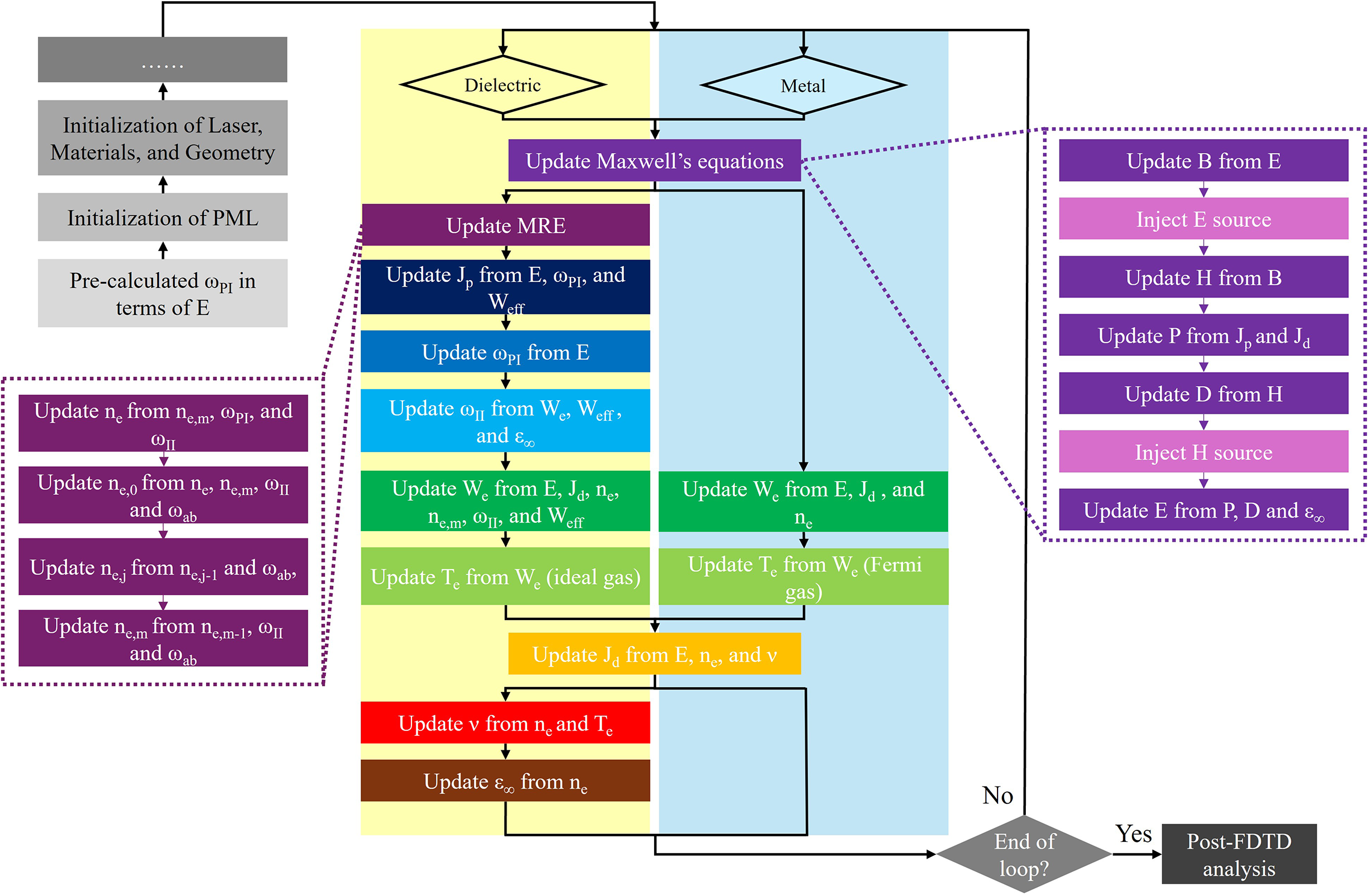
Section 2.1 describes the auxiliary differential equation (ADE) form of the FDTD, which is the foundation of the framework. The ionization processes and free-electron dynamics for dielectrics are described in Sections 2.2–2.4. The optical response in dielectrics and metals is presented in Section 2.5. Collisional effects for dielectrics are examined in Section 2.6. Finally, the transient distinct treatments required for modeling Ohmic heating in dielectrics and metals are presented in Section 2.7. A schematic overview of the proposed workflow is shown in Figure 1 in Section 2. For clarity, the initialization procedures are not shown in full; the figure highlights only the major transient parameters updated within the main simulation loop.
Illustration of the framework. The initialization procedures are not present in full, and only major transient parameters are shown in the workflow.

Figure 1 Long description
The workflow is organized into three main sections.
1. Initialization (Top-Left): A vertical stack of grey boxes starting from the bottom with Pre-calculated omega sub P I in terms of E, moving up to Initialization of P M L, and Initialization of Laser, Materials, and Geometry.
2. Main Processing Core (Center): Two parallel columns labeled Dielectric (yellow background) and Metal (blue background).
- Both paths start with Update Maxwell's equations.
- The Dielectric path includes: Update M R E; Update J sub p from E, omega sub P I, and W sub eff; Update omega sub P I from E; Update omega sub I I from W sub e, W sub eff, and epsilon sub infinity; Update W sub e from E, J sub d, n sub e, n sub e,m, omega sub I I, and W sub eff; Update T sub e from W sub e (ideal gas).
- The Metal path includes: Update W sub e from E, J sub d, and n sub e; Update T sub e from W sub e (fermi gas).
- The paths converge to: Update J sub d from E, n sub e, and v; Update v from n sub e and T sub e; Update epsilon sub infinity from n sub e.
3. Expanded Sub-processes (Dashed Boxes):
- Left Box (linked to Dielectric updates): A sequence of four steps updating n sub e, n sub e,0, n sub e,j, and n sub e,m based on various parameters including omega sub I I and omega sub a b.
- Right Box (linked to Maxwell's equations): A seven-step sequence: Update B from E; Inject E source; Update H from B; Update P from J sub p and J sub d; Update D from H; Inject H source; Update E from P, D and epsilon sub infinity.
4. Termination (Bottom-Right): A decision diamond asks End of loop? If No, it loops back to the top. If Yes, it proceeds to Post-F D T D analysis.
2.1 FDTD algorithm
The FDTD is well suited for modeling electromagnetic wave propagation and interaction inside the materials because it directly solves Maxwell’s equations on a staggered Yee grid[ Reference Yee and Chen 43 ] by central-difference approximation with second-order accuracy in both space and time[ Reference Taflove and Hagness 47 ]. The governing equations are as follows:

where
$\mathbf{E}$
 and
$\mathbf{H}$
 denote the electric and magnetic fields; and
$\mathbf{D}$
 and
$\mathbf{B}$
 are the corresponding electric and magnetic flux densities, related through the constitutive relations
$\mathbf{D}={\epsilon}_0{\epsilon}_{\infty}\mathbf{E}+\mathbf{P}$
 and
$\mathbf{B}={\mu}_0{\mu}_{\mathrm{r}}\mathbf{H}$
 . The total current density
$\mathbf{J}$
 contains both the effective ionization current
${\mathbf{J}}_{\mathrm{p}}$
 associated with PI energy loss[
Reference Rae and Burnett
48
] and the Drude current
${\mathbf{J}}_{\mathrm{d}}$
 [
Reference Kashiwa and Fukai
49
], which are discussed in Sections 2.2 and 2.5, respectively.
To implement these equations numerically, the FDTD scheme discretizes space and time on the Yee lattice. For clarity of illustration, consider a one-dimensional (1D) configuration where the fields vary only along the
$x$
 direction (assuming TE
${}_z$
 mode). The discrete update equations become

where the superscripts
$t$
 and subscripts
$x$
 indicate the current discrete time point and spatial location, respectively, and
$\Delta t$
 and
$\Delta x$
 are the time step and grid spacing, respectively, which satisfy the Courant–Friedrichs–Lewy (CFL) stability condition[
Reference Lewy, Friedrichs and Courant
50
]. In the following theoretical formulations, whenever a time derivative is required, the corresponding FDTD discretization will also be provided for implementation convenience.
2.2 Photoionization
Since the dielectric usually has a large band gap and almost no absorption at room temperature, it requires great amount of electromagnetic energy to ionize electrons from the bound states. The behaviors of PI are determined by the Keldysh parameter[ Reference Keldysh 38 ], defined as follows:

where
$\omega$
 is the laser frequency,
${m}^{\ast }$
 is the reduced mass given by effective electron and hole masses
$1/\left(1/{m}_{\mathrm{e}}^{\ast }+1/{m}_{\mathrm{h}}^{\ast}\right)$
 ,
${W}_0$
 is the intrinsic ionization energy and
$e$
 is the elementary charge. When
$\gamma \ll 1$
 , TI dominates. This requires a high-strength electric field so that the bound potential wells in the quasi-classical atomic model are tilted by the external strong field, which increases the probability of freeing an electron. When
$\gamma \gg 1$
 , MPI dominates. A single photon cannot give the electron enough energy to get into the conduction band; thus, the electron can briefly stay in some intermediate excited state and absorb multiple photons to be further excited. This model assumes each atom or molecule only ionizes one electron.
For brevity in the following expressions, we follow the work of Balling and Schou[
Reference Balling and Schou
15
], Tien et al.
[
Reference Tien, Backus, Kapteyn, Murnane and Mourou
27
] and Zhang et al.
[
Reference Zhang, Menoni, Gruzdev and Chowdhury
35
] by introducing the variables
${\gamma}_1={\gamma}^2/\left(1+{\gamma}^2\right)$
 and
${\gamma}_2=1/\left(1+{\gamma}^2\right)$
 . The effective band gap in units of the photon energy is given by

and the PI rate
${\omega}_{\mathrm{PI}}$
 is then

where
$\mathbb{K}$
 and
$\mathbb{E}$
 are complete elliptic integrals of the first and second kind,
$\Phi$
 is the Dawson integral and

The mixed ionization mechanism described by Keldysh is successfully employed in many recent works[ Reference Kaiser, Rethfeld, Vicanek and Simon 19 , Reference Tien, Backus, Kapteyn, Murnane and Mourou 27 , Reference Petrov and Davis 31 , Reference Chimier, Utéza, Sanner, Sentis, Itina, Lassonde, Légaré, Vidal and Kieffer 33 – Reference Smith, Su, Zhang, Varin, Gruzdev and Chowdhury 37 ], although several studies[ Reference Kaiser, Rethfeld, Vicanek and Simon 19 , Reference Tien, Backus, Kapteyn, Murnane and Mourou 27 , Reference Petrov and Davis 31 , Reference Chimier, Utéza, Sanner, Sentis, Itina, Lassonde, Légaré, Vidal and Kieffer 33 , Reference Sun, Zhu and Lin 34 , Reference Charpin, Ardaneh, Morel, Giust and Courvoisier 36 ] directly adopted the original expression and perpetuated the misprinted numerical prefactor 2 appearing in the original publication[ Reference Keldysh 38 ].
Moreover, Keldysh’s PI model simplifies the electronic structure of solids. Firstly, the multi-valence-band structure is not explicitly included. Although the valence band dispersion can, in principle, influence the TI rate[
Reference Gruzdev
51
], studies of the multi-valence-band Keldysh formulation in crystalline semiconductors show that the heavy-hole (HH), light-hole (LH) and split-off (SO) bands at the
$\Gamma$
 point differ by only
$0.01$
 –
$0.1\kern0.22em \mathrm{eV}$
 and yield nearly identical ionization rates when evaluated using either parabolic or non-parabolic band relations[
Reference Gruzdev, Austin, Sergaeva and Chowdhury
52
]. In the present work, the materials are wide-bandgap amorphous dielectrics where the valence band is broad and does not exhibit a well-resolved HH/LH/SO substructure; thus, the standard non-parabolic single-valence-band Keldysh PI rate is a sufficiently accurate approximation. Secondly, the Keldysh PI model does not include intermediate excited bound states within the bandgap. Ionization is treated as a direct transition from the valence band to the conduction band. As a result, possible multi-photon resonances are not captured. Nevertheless, for the near-infrared (near-IR) to mid-infrared sub-ps pulses considered in this work – where the ionization dynamics is governed primarily by tunneling and MPI – the standard Keldysh rate remains a reliable and widely used approximation[
Reference Popruzhenko
53
].
On the other hand, the Keldysh formalism is formulated in terms of cycle-averaged quantities, whereas FDTD resolves the field evolution on a fully time-dependent, sub-cycle basis. The Keldysh’s PI model assumes complete knowledge of the instantaneous laser field – its amplitude, phase and frequency – at every time and spatial location. In contrast, the FDTD method provides the electric field only at discrete time steps and only for times preceding the current update. Thus, during the rising edge of a given cycle in the pulse, the amplitude is not yet known within the FDTD framework. Therefore, we store the electric field at each grid point over one full optical cycle and input the maximum value in that interval as the amplitude
$E_{\mathrm{cyc}}$
 in Equation (3) to the Keldysh rate calculation[
Reference Zhang, Menoni, Gruzdev and Chowdhury
35
]. This approximation is appropriate for multi-cycle pulses but becomes unreliable for high-intensity few-cycle pulses[
Reference Gruzdev and Sergaeva
54
].
Due to the complexity of the Keldysh formulation, the PI rate is pre-computed and tabulated over an electric field amplitude range from
$1.6\times {10}^3$
 to
$1.0\times {10}^{11}\kern0.22em \mathrm{V}/\mathrm{m}$
 prior to the FDTD simulation, as shown in Figure 1. The field is sampled uniformly with a step size of
$10\kern0.22em \mathrm{V}/\mathrm{m}$
 . Pre-tabulation eliminates costly transient evaluations during the time-domain simulation and is significantly more time- and cost-efficient. The summation of
$Q\left(\gamma, {W}_{\mathrm{eff}}\right)$
 in Equation (6) is evaluated with 1000 terms, as 500 terms already produce excellent convergence[
Reference Smith, Su, Zhang, Varin, Gruzdev and Chowdhury
37
].
Lastly, the effective PI loss current
${\mathbf{J}}_{\mathrm{p}}$
 is modeled as follows[
Reference Peñano, Sprangle, Hafizi, Manheimer and Zigler
29
,
Reference Zhang, Menoni, Gruzdev and Chowdhury
35
,
Reference Rae and Burnett
48
]:

where
$f$
 is a depopulation factor, which is discussed in Section 2.4, and
$\mathbf{E}$
 is the maximum electric field evaluated over the nearest cycle.
2.3 Impact ionization
A following II process after there are enough seed electrons generated by PI would happen to further promote electrons in dielectrics. The II rate also suggested by Keldysh[ Reference Keldysh 55 ] is calculated in terms of electron energy as shown below:

where
$W$
 is the energy of an electron,
${W}_{\mathrm{ion}}$
 is the threshold ionization energy, which is defined as
${\beta}_0{W}_0$
 , where
${\beta}_0=\left(1+2{m}_{\mathrm{e}}^{\ast }/{m}_{\mathrm{h}}^{\ast}\right)/\left(1+{m}_{\mathrm{e}}^{\ast }/{m}_{\mathrm{h}}^{\ast}\right)$
 , and
${\alpha}_0$
 is a rate constant, typically taken as 1.3–1.5
${\mathrm{fs}}^{-1}$
 for fused silica in other works[
Reference Stuart, Feit, Herman, Rubenchik, Shore and Perry
12
,
Reference Peñano, Sprangle, Hafizi, Manheimer and Zigler
29
,
Reference Petrov and Davis
31
,
Reference Chimier, Utéza, Sanner, Sentis, Itina, Lassonde, Légaré, Vidal and Kieffer
33
,
Reference Zhang, Menoni, Gruzdev and Chowdhury
35
]. In the absence of data, this value is often assumed for other wide-bandgap dielectrics as well. However, in the present work, it is approximated by the following:

where
${m}_{\mathrm{e}}={m}_{\mathrm{e}}^{\ast }/{m}_0$
 and
${m}_{\mathrm{h}}={m}_{\mathrm{h}}^{\ast }/{m}_0$
 are the relative effective electron mass and hole mass, respectively, and
${A}_{\mathrm{c}}{,}\ {A}_{\mathrm{v}}$
 are overlap integrals between the initial and final states of the conduction band and valence band electrons promoted to the conduction band, respectively[
Reference Charpin, Ardaneh, Morel, Giust and Courvoisier
36
,
Reference Ridley
56
]. When the corrected Keldysh PI rate is employed, directly adopting
${\alpha}_0=1.5\ {\mathrm{fs}}^{-1}$
 used in previous simulations[
Reference Peñano, Sprangle, Hafizi, Manheimer and Zigler
29
,
Reference Petrov and Davis
31
,
Reference Chimier, Utéza, Sanner, Sentis, Itina, Lassonde, Légaré, Vidal and Kieffer
33
], where the PI rate was underestimated, may lead to an overestimation of the II rate. Although good agreement with experiments was reported, the reduced PI contribution suggests that II was effectively increased to compensate.
In addition, a Maxwell–Boltzmann velocity distribution is usually assumed for the electron population[ Reference Peñano, Sprangle, Hafizi, Manheimer and Zigler 29 , Reference Petrov and Davis 31 , Reference Zhang, Menoni, Gruzdev and Chowdhury 35 ]. This approximation neglects the strongly non-thermal, ballistic character of laser-driven carriers, especially in the high-energy tail that is primarily responsible for initiating II. To avoid assuming a thermal equilibrium distribution for the conduction band electrons, we employ an MRE formulation[ Reference Rethfeld, Ivanov, Garcia and Anisimov 25 , Reference Rethfeld 39 ] that tracks the population of electrons in discrete energy levels evolving through ionization and absorption processes, as described in the next section.
2.4 Electron dynamics
Instead of employing an SRE[ Reference Bloembergen 40 ], which usually overestimates the importance of II during the excitation process[ Reference Balling and Schou 15 ], we decompose the II term using an MRE formulation in order to capture the dominant non-thermal characteristics of the carrier dynamics under strong-field excitation[ Reference Rethfeld, Ivanov, Garcia and Anisimov 25 , Reference Christensen and Balling 32 , Reference Sun, Zhu and Lin 34 , Reference Rethfeld 39 ]. The evolution of the electron populations in the conduction band is governed by the following:

where
${n}_{\mathrm{e}}$
 is the total conduction band electron density,
${n}_{\mathrm{e},0}$
 is the population at the lowest energy level, m denotes the highest energy level in the conduction band where II happens,
${\omega}_{\mathrm{ab}}$
 is the one-photon absorption rate and
${\tau}_{\mathrm{r}}$
 is the recombination time. Each level is separated by the one-photon energy.
The first equation corresponds to the conventional SRE, except that the total carrier density
${n}_{\mathrm{e}}$
 entering the II term is replaced by the highest-energy MRE level
${n}_{\mathrm{e},m}$
 . The total number of conduction band levels is approximated by
${W}_{\mathrm{ion}}/\left(\mathrm{\hslash}\omega \right)$
 . The second equation updates the population of the highest level m, which gains electrons from level m–1 and loses electrons through II. The intermediate levels simply gain electrons from the level below and lose electrons to the level above, governed by an energy-dependent
${\omega}_{\mathrm{ab}}$
 . The final equation ensures that the change in the floor-level population remains synchronized with the change in the total density due to ionization and recombination, plus the electrons coming back from the highest level. This MRE formulation enables the model to capture the non-thermal high-energy tail of the electron population, which plays a critical role in II. However, electron emission into vacuum is not included in the present model. Although the higher MRE levels may correspond to energies exceeding the electron affinity of the material, emission occurs only at the surface, and electrons generated in the bulk are assumed to remain within the material due to their short mean free path (a few nm for electrons with energies of the order of 10 eV)[
Reference Ridzel, Astašauskas and Wolfgang
57
].
The parameter
$f$
 is a depopulation factor defined as
$f=1-{n}_{\mathrm{e}}/\left({n}_0-{n}_{\mathrm{e}}\right)$
 , where
${n}_0$
 is the valence band electron density, which ensures that the PI contribution remains valid only when the conduction band electron population is much smaller than the valence band population – consistent with the fundamental assumption of Keldysh’s PI model. Further discussion can be found in our previous work[
Reference Zhang, Menoni, Gruzdev and Chowdhury
35
].
The forward Euler discretization with first-order accuracy is applied to MRE formulation, as shown below, with the electron population in the energy ladder being updated sequentially from lower to higher energy levels (from j = 0 to j = m) within each time step:

The convergence tests were performed, showing negligible (less than 0.7%) differences in electron density dynamics compared with a centered discretization. Therefore, the forward Euler scheme is adopted here for simplicity.
2.5 Optical response
The optical response of free electrons in a material is commonly described by the Drude model, which can be viewed as the zero-resonance limit of the more general Lorentz–Drude oscillator model[ Reference Benavides-Cruz, Calderón-Ramón, Gomez-Aguilar, Rodríguez-Achach, Cruz-Orduña, Laguna-Camacho, Morales-Mendoza, Enciso-Aguilar, Pérez-Meana, Escalante-Martínez, López-Calderón and Juárez-Morales 58 ]. The newly generated conduction band electrons by strong-field ionization in a dielectric behave similarly to free electrons in a metal. The complex permittivity is expressed as follows:

where
${\omega}_{\mathrm{p},\mathrm{e}}=\sqrt{n_{\mathrm{e}}{e}^2/\left({\epsilon}_0{m}_{\mathrm{e}}^{\ast}\right)}$
 is the free-electron plasma frequency and
$\nu$
 is the collision rate.
For metals,
${\epsilon}_{\infty }$
 represents the background permittivity arising from interband transitions and is typically obtained from optical data, although some works take
${\epsilon}_{\infty }$
 to be unity[
Reference Pernice, Payne and Gallagher
59
]. In wide-bandgap dielectrics,
${\epsilon}_{\infty }$
 is typically equal to the linear relative permittivity
${\epsilon}_{\mathrm{r}}$
 in the absence of free carriers in the near-IR regime. Once strong-field ionization generates a significant population of conduction band electrons, the contribution of neutral atoms to the polarizability decreases, and the transient optical response begins to approach a metal-like behavior. Within the low-frequency neutral-polarizability approximation adopted in this work, the background permittivity is modified as follows[
Reference Peñano, Sprangle, Hafizi, Manheimer and Zigler
29
]:

where
${\omega}_{\mathrm{p},\mathrm{n}}$
 is defined by
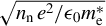
$\sqrt{n_{\mathrm{n}}\kern0.1em {e}^2/{\epsilon}_0{m}_{\mathrm{e}}^{\ast }}$
 , with
${n}_{\mathrm{n}}$
 being the neutral-particle density. When no free electrons are present,
${\epsilon}_{\mathrm{r}}$
 is known, and thus the effective resonance constant
${\Omega}_0$
 can be easily obtained from Equation (13).
To integrate the permittivity in frequency domain into time domain, an ADE technique is applied[
Reference Kashiwa and Fukai
49
,
Reference Benavides-Cruz, Calderón-Ramón, Gomez-Aguilar, Rodríguez-Achach, Cruz-Orduña, Laguna-Camacho, Morales-Mendoza, Enciso-Aguilar, Pérez-Meana, Escalante-Martínez, López-Calderón and Juárez-Morales
58
]. The ADE formulation is particularly effective for representing material dispersion and enables absorption to be incorporated naturally through Drude current density terms
${\mathbf{J}}_{\mathrm{d}}$
 , expressed as follows:

In the FDTD scheme, this equation is integrated in time using a semi-implicit (trapezoidal) update. For the 1D
$z$
 -component along the
$x$
 direction, the Drude current can be written as follows[
Reference Pernice, Payne and Gallagher
59
]:

2.6 Collision
Collisions are the primary mechanism for transferring energy and establishing thermal equilibrium in laser-excited materials. During ultrashort interactions, electrons acquire energy much faster than ions or phonons, making electron–neutron (e–n) and electron–ion (e–i) collisions the dominant contributors to the transient momentum-relaxation rate. Electron–phonon (e–p) and electron–defect (e–d) scattering both influence the effective electron conductivity. However, accurately modeling these mechanisms in amorphous materials is difficult and currently limited by insufficient experimental data[ Reference Zhang, Menoni, Gruzdev and Chowdhury 35 ].
The e–n collision frequency
${\nu}_{\mathrm{en}}$
 is commonly approximated by the ratio of thermal velocity to mean free path, assuming a Maxwell–Boltzmann distribution of electron velocities. It is written as follows[
Reference Balling and Schou
15
,
Reference Lee and More
60
–
Reference Wang, Du and Huo
62
]:

where
$\sigma$
 is the scattering cross-section,
${n}_{\mathrm{n}}$
 is the neutral density,
${u}_{\mathrm{th}}$
 is the thermal velocity, defined as
$\sqrt{3{k}_{\mathrm{B}}{T}_{\mathrm{e}}/{m}_{\mathrm{e}}^{\ast }}$
 , and
${T}_{\mathrm{e}}$
 is the electron temperature.
Encounters between electrons and ions are well described by the Spitzer collision model, in which the ions are treated as stationary scattering centers and the test electron experiences only small-angle deflections. The e–i collision frequency is as follows[ Reference Balling and Schou 15 , Reference Huba 61 , Reference Callen 63 ]:

where
${Z}_{\mathrm{i}}$
 is the ionization state of nuclei and
$\ln \Lambda =\ln \left({b}_{\mathrm{max}}/{b}_{\mathrm{min}}\right)$
 is the Coulomb logarithm, with
${b}_{\mathrm{max}}\ge {b}_{\mathrm{min}}$
 . The maximum impact parameter is taken to be the Debye length,
${b}_{\mathrm{max}}={\lambda}_{\mathrm{D}}$
 . The minimum impact parameter[
Reference Lee and More
60
] is determined by either the classical distance of closest approach:

or by quantum uncertainty principles when the classical distance of the closest approach is smaller than the de Broglie wavelength:

where
${u}_{\mathrm{fe}}$
 is the characteristic Fermi electron velocity, defined as
${u}_{\mathrm{fe}}=\sqrt{2{k}_{\mathrm{B}}{T}_{\mathrm{e}}/{m}_{\mathrm{e}}^{\ast }}$
 . In practice, the minimum impact parameter is chosen as
${b}_{\mathrm{min}}=\max \left({b}_{\mathrm{min}}^{\mathrm{cl}},{b}_{\mathrm{min}}^{\mathrm{qm}}\right)$
 .
However, when the electron temperature decreases to a few eV in a solid-density plasma, the Coulomb logarithm
$\ln \Lambda$
 may become negative, indicating that the assumption of dominant small-angle scattering underlying Equation (17) is no longer valid. In this regime, the impact parameter
$b$
 becomes smaller than
${b}_{\mathrm{min}}$
 , and classical ‘hard’ collisions with large-angle deflections dominate the e–i interaction. The corresponding hard collision frequency can be approximated as[
Reference Zhang, Menoni, Gruzdev and Chowdhury
35
,
Reference Callen
63
]

reflecting the increased importance of close binary encounters.
The
$\ln \Lambda$
 is evaluated dynamically during the simulation, and the
${\nu}_{\mathrm{ei}}$
 term is disabled when
$\ln \Lambda <0$
 . For laser-excited wide-bandgap dielectrics, the transient total collision rate is approximated by the following sum[
Reference Lee and More
60
,
Reference Peñano, Sprangle, Hafizi, Manheimer and Zigler
29
,
Reference Chimier, Utéza, Sanner, Sentis, Itina, Lassonde, Légaré, Vidal and Kieffer
33
,
Reference Zhang, Menoni, Gruzdev and Chowdhury
35
]:

However, for metals that have a high intrinsic conduction band electron density and a dense ionic lattice, instead of resolving a transient collision rate based on electron or neutral density, we use a constant effective collision rate extracted from measured complex refractive index
$\left(n,\kappa \right)$
 via the Drude model. This approach accurately reproduces absorption and reflectivity at the laser wavelength of interest and is sufficient for ultrafast energy deposition and damage modeling without requiring broadband dispersion resolution in the present work.
A distinction is made between the treatment of electron distributions in different processes. The thermal assumption used in Equations (16)–(18) is appropriate for e–n and e–i collisions because the rates depend mainly on the bulk thermal population. In contrast, II is highly sensitive to the high-energy tail of the electron distribution, which deviates strongly from thermal equilibrium during ultrafast excitation. Therefore, an MRE framework is applied to resolve the non-thermal conduction band population, ensuring that the energetic electron tail driving II is accurately captured.
2.7 Ohmic heating
When the laser field accelerates free or conduction band electrons, the electromagnetic energy is partially converted into thermal energy through Ohmic heating. In the FDTD scheme, the instantaneous power density is evaluated from the microscopic current and electric field. For dielectric regions, a portion of this absorbed energy is consumed by II[ Reference Peñano, Sprangle, Hafizi, Manheimer and Zigler 29 , Reference Zhang, Menoni, Gruzdev and Chowdhury 35 ]:

where
${W}_{\mathrm{e}}$
 denotes the average electron energy per electron and
${n}_{\mathrm{e},\mathrm{col}}$
 is the density of excited electrons by II. The average electron energy then is computed in the FDTD as follows:

Here
${E}_{{x}}^{{t}+\Delta {t}/2}$
 and
${n}_{\mathrm{e},\mathrm{col}}^{{t}+\Delta {t}/2}$
 denote midpoint values obtained by averaging the corresponding quantities at the adjacent full time steps. The effective energy is evaluated at the end of the interval, that is,
${W}_{\mathrm{eff}}^{{t}+\Delta {t}/2}\approx {W}_{\mathrm{eff}}^{{t}+\Delta {t}}$
 .
The electron temperature is obtained from the appropriate equation of state. For dielectrics the conduction electrons are assumed to behave as an ideal gas[
Reference Peñano, Sprangle, Hafizi, Manheimer and Zigler
29
,
Reference Zhang, Menoni, Gruzdev and Chowdhury
35
], whereas for metals they form a degenerate Fermi gas, and their thermodynamic properties must therefore be described using the Fermi energy[
Reference Chimier, Utéza, Sanner, Sentis, Itina, Lassonde, Légaré, Vidal and Kieffer
33
,
Reference Ashcroft and Mermin
64
]
$\ {E}_{\mathrm{F}}={\mathrm{\hslash}}^2{\left(3{\pi}^2{n}_{\mathrm{e}}\right)}^{2/3}/\left(2{m}_{\mathrm{e}}^{\ast}\right)$
 . Therefore, the relation between electron energy and electron temperature is as follows:

where
${\gamma}_{\mathrm{Ce}}={\pi}^2{k}_{\mathrm{B}}^2/\left(2{E}_{\mathrm{F}}\right)$
 is the electron heat capacity constant[
Reference Jiang and Tsai
30
]. The resulting electron temperature is usually lower than that predicted by an ideal gas model, making the Fermi gas description essential for realistic ultrafast heating of metals.
3 Technique
3.1 Uniaxial perfectly matched layer
To avoid scattered waves being reflected from the domain boundaries, we employ a uniaxial perfectly matched layer (UPML) technique[
Reference Taflove and Hagness
47
,
Reference Inan and Marshall
65
,
Reference Sacks, Kingsland, Lee and Lee
66
] based on the perfectly matched layer (PML) technique introduced by Berenger[
Reference Berenger
67
]. The UPML consists of an artificial absorbing medium placed at the edges of the computational domain that introduces strong attenuation while producing negligible reflection. This is achieved by enforcing impedance matching at the interface between the physical domain and UPML by multiplying an anisotropic complex tensor
$\overline{s}$
 to both the permittivity and permeability:

with

where
${\kappa}_{{j}}$
 is the scaling parameter (often chosen as
${\kappa}_{{j}}=1$
 ) and
${\sigma}_{{j}}$
 is the artificial conductivity profile, which is graded polynomially from zero to some maximum value at the outer UPML boundary to minimize reflections[
Reference Berenger
67
]. The explicit current term
$\mathbf{J}$
 is ignored as the UPML is implemented in vacuum.
By discretizing Equation (25) in one spatial dimension along
$x$
 , and noting that in this case
${s}_{{y}}={s}_{{z}}=1$
 , the resulting UPML updates take the following form:

In the 1D case, the update equations for
$E$
 and
$B$
 reduce to their standard forms and are unchanged from the non-PML region. Extension to two dimensions is straightforward and follows by applying the complex tensors independently along each spatial axis.
3.2 Total field/scattered field
To inject the laser pulse without placing its full spatial profile in the simulation domain as an initial condition, we employ the TFSF technique. The TFSF mechanism is also illustrated using the 1D TE
${}_z$
 case for simplicity. In this setting, the incident field is introduced at the TFSF boundary
$x={x}_{\mathrm{TFSF}}$
 by modifying the discrete curl operators that cross this interface. At the TFSF interface,
${B}_{{{x}}_{\mathrm{TFSF}}+\Delta {x}/2}$
 is a total-field quantity. Therefore it should be updated using only the total-field quantity, requiring adding the known
${E}_{\mathrm{inc}}$
 to the scattered-field quantity
${E}_{{{x}}_{\mathrm{TFSF}}}$
 . Similarly, the correction is made to
${H}_{{{x}}_{\mathrm{TFSF}}+\Delta {x}/2}$
 , and the resulting 1D TFSF update expression in the FDTD is as follows:

In the actual 2D simulation, we employ a line TFSF boundary parallel to the y-axis that supports an obliquely incident Gaussian pulse propagating along the x-axis. A similar modification is made as in Equation (28). To account for the angle of incidence
$\theta$
 , the temporal delay of the incident wavefront along the TFSF boundary is computed analytically to impose the desired angle of incidence and transverse beam profile:

where
${y}_0$
 is the transverse center of the pulse,
$g(t)$
 denotes the temporal envelope and
${w}_0$
 is the Gaussian spot radius. The
$\sin \theta$
 term introduces the appropriate time delay of the same wavefront along the boundary at the desired angle of incidence, while the
$\cos \theta$
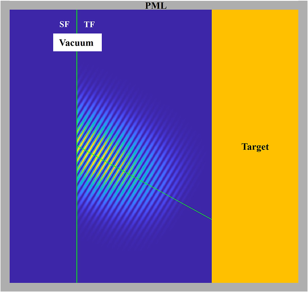
 factor accounts for the projection of the Gaussian beam profile onto the TFSF boundary. This approach preserves both the temporal and spatial characteristics of the incident Gaussian pulse and enables stable injection of obliquely incident beams extending to the ps scale. A schematic of the TFSF injection geometry and source profiles is shown in Figure 2.
An illustration of the spatial simulation domain with TFSF pulse injection and a PML at the domain boundaries is shown. The blue region represents vacuum, while the yellow region denotes the target. The region to the left of the injection boundary corresponds to the SF region, whereas the region to the right corresponds to the TF region.

4 Simulation setup
We simulate a
$1057$
 $\mathrm{nm}$
 , 500
$\mathrm{fs}$
 (full width at half maximum (FWHM)), s-polarized laser pulse with a sinusoidal temporal envelope and a Gaussian focal spot, incident at
$77.2{}^{\circ}$
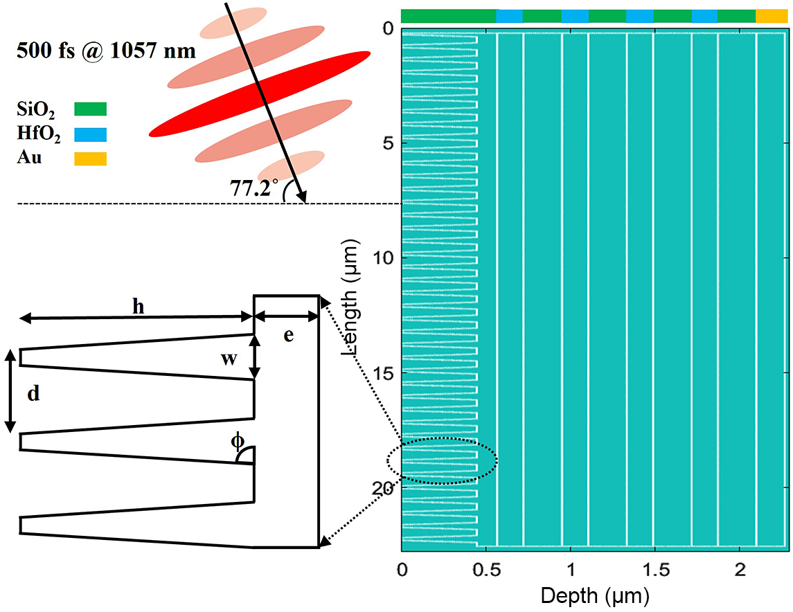
 onto a hybrid multilayer grating, as shown in Figure 3. The grating structure follows the design of Néauport et al.
[
Reference Néauport, Bonod, Hocquet, Palmier and Dupuy
68
,
Reference Néauport, Bonod, Hocquet, Palmier, Lavastre, Baclet and Dupuy
69
] and consists of a 580
$\mathrm{nm}$
 SiO2 top layer deposited on four HfO
${}_2$
 (157
$\mathrm{nm}$
 )/SiO
${}_2$
 (232
$\mathrm{nm}$
 ) pairs, which in turn rest on a 170 nm Au base layer. In the original design, a
$20\ \mathrm{nm}$
 Cr transition layer is present beneath the Au layer; however, it is not included in the present simulations, as the electromagnetic field penetration beyond the Au layer is negligible. The FDTD computational domain spans
$22.8\ \unicode{x3bc} \mathrm{m}\times 3.6\kern0.22em \unicode{x3bc} \mathrm{m}$
 with a uniform spatial resolution of 12
$\mathrm{nm}$
 in both directions. The total simulation time is 1.1
$\mathrm{ps}$
 and the temporal step is 0.0283 fs. The laser pulse is injected from the left-hand vacuum region by the TFSF boundary. The grating pillar has a bottom duty cycle of 0.473 and a line density of 1780 lines/
$\mathrm{mm}$
 , with a sidewall angle of
$78.2{}^{\circ}$
 . The pillar height is 456
$\mathrm{nm}$
 , leaving a 124
$\mathrm{nm}$
 residual layer.
Schematic illustration of the simulation setup and grating geometry. A
$1057\ \mathrm{nm}$
 ,
$500\ \mathrm{fs}$
 (FWHM), s-polarized laser pulse with a sinusoidal temporal envelope and a Gaussian focal spot is incident at an angle of
$77.2{}^{\circ}$
 . The hybrid multilayer grating consists of
$170\ \mathrm{nm}$
 Au/(232
$\mathrm{nm}$
 SiO
${}_2$
 ${/}157~\mathrm{nm}$
 HfO
${}_2$
 )
${}^4$
 /
$580\ \mathrm{nm}$
 SiO
${}_2$
 , with the colors corresponding to the materials (SiO
${}_2$
 , green; HfO
${}_2$
 , blue; Au, yellow) shown in the top right. The enlarged schematic on the left defines the grating geometric parameters, including the pillar height
$h=456\kern0.22em \mathrm{nm}$
 , period
$d=562\kern0.22em \mathrm{nm}$
 , pillar bottom width
$w=257\kern0.22em \mathrm{nm}$
 , residual thickness
$e=124\kern0.22em \mathrm{nm}$
 and sidewall angle
$\phi =78.2{}^{\circ}$
 .

Figure 3 Long description
A multi-panel schematic detailing a simulation setup.
* Top-Left: A laser pulse labeled 500 f s at 1057 n m is shown as a series of red ellipses with a central black arrow indicating an incident angle of 77.2 degrees relative to the horizontal surface. A legend identifies S i O sub 2 as green, H f O sub 2 as blue, and A u as yellow.
* Right: A large cross-sectional plot shows the grating structure. The vertical axis is Length in micrometers from 0 to 20. The horizontal axis is Depth in micrometers from 0 to 2. The surface at Depth 0 consists of a periodic pillar structure. A color bar at the top indicates the material sequence: green (S i O sub 2), blue (H f O sub 2), blue, blue, blue, and yellow (A u) at the far right.
* Bottom-Left: An enlarged view of the grating pillars with geometric labels.
- h: pillar height of 456 n m.
- d: period of 562 n m.
- w: pillar bottom width of 257 n m.
- e: residual thickness of 124 n m.
- phi: sidewall angle of 78.2 degrees.
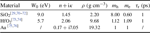
The material parameters are shown in the Table 1. The recombination time is assumed to be 1 ps for both SiO
${}_2$
 and HfO
${}_2$
 . Although recombination time of approximately 220 fs for SiO
${}_2$
 has been reported in the literature based on multi-parameter fit of LIDT data[
Reference Mero, Liu, Rudolph, Ristau and Starke
77
], we adopt a recombination time of 1 ps[
Reference Xu, Zou, Chen, Zhang, Wang, Jin, Kong, Cao, Chen and Shao
41
] for both SiO
${}_2$
 and HfO
${}_2$
 . This choice is supported by time-resolved pump–probe microscopy of damage and ablation of SiO
${}_2$
 /HfO
${}_2$
 layers in our previous works, which directly captures the dynamics of density of electron–hole plasma in such layers, showing pronounced reduction in probe light absorption due to lowering of plasma density in ps time scales[
Reference Talisa, Tripepi, Harris, AlShafey, Krebs, Davenport, Randel, Menoni and Chowdhury
78
,
Reference Talisa, Alshafey, Tripepi, Krebs, Davenport, Randel, Menoni and Chowdhury
79
].
Material properties used in simulations.

Table 1 Long description
The table consists of seven columns and four rows including the header.
* Column 1: Material.
* Column 2: E sub g (e V).
* Column 3: n plus i kappa.
* Column 4: rho (g cm super minus 3).
* Column 5: m sub h.
* Column 6: m sub e.
* Column 7: tau sub r (p s).
Data rows:
1. S i O sub 2: 9.0, 1.45, 2.20, 8.00, 0.60, 1.
2. H f O sub 2: 5.7, 2.06, 9.68, 1.12, 1.09, 1.
3. A u: forward slash, 0.17 plus i 7.05, 19.32, 1, 1, forward slash.
Moreover, since no overlap integral data are available for amorphous SiO
${}_2$
 , we adopt a reduced, direction-averaged value based on the crystalline Si[
Reference Sano and Yoshii
80
], which reported
${A}_{\mathrm{v}}^2$
 from 0 to 0.05 and
${A}_{\mathrm{c}}^2$
 from 0 to 0.6. The effective overlap integrals in SiO
${}_2$
 are expected to be smaller than those of Si, owing to the absence of long-range periodicity, the larger band gap and the reduced coherence of electronic wavefunctions in the amorphous phase. Also, Charpin et al.
[
Reference Charpin, Ardaneh, Morel, Giust and Courvoisier
36
] reported fitted
${A}_{\mathrm{v}}^2$
 and
${A}_{\mathrm{c}}^2$
 both equal to
$0.027$
 for SiO
${}_2$
 , although the PI rate expression is misprinted. On this basis, we use values of
${A}_{\mathrm{v}}^2=0.025$
 and
${A}_{\mathrm{c}}^2=0.2$
 , which provide reasonable order-of-magnitude estimates for amorphous SiO
${}_2$
 .
5 Results and discussion
5.1 Distribution
We performed simulations over incident fluences ranging from
$2.5$
 to
$3.7\;\mathrm{J}/{\mathrm{cm}}^2$
 to investigate the nonlinear field enhancement, carrier generation and energy deposition dynamics in the grating. At a fluence of
$3.2\;\mathrm{J}/{\mathrm{cm}}^2$
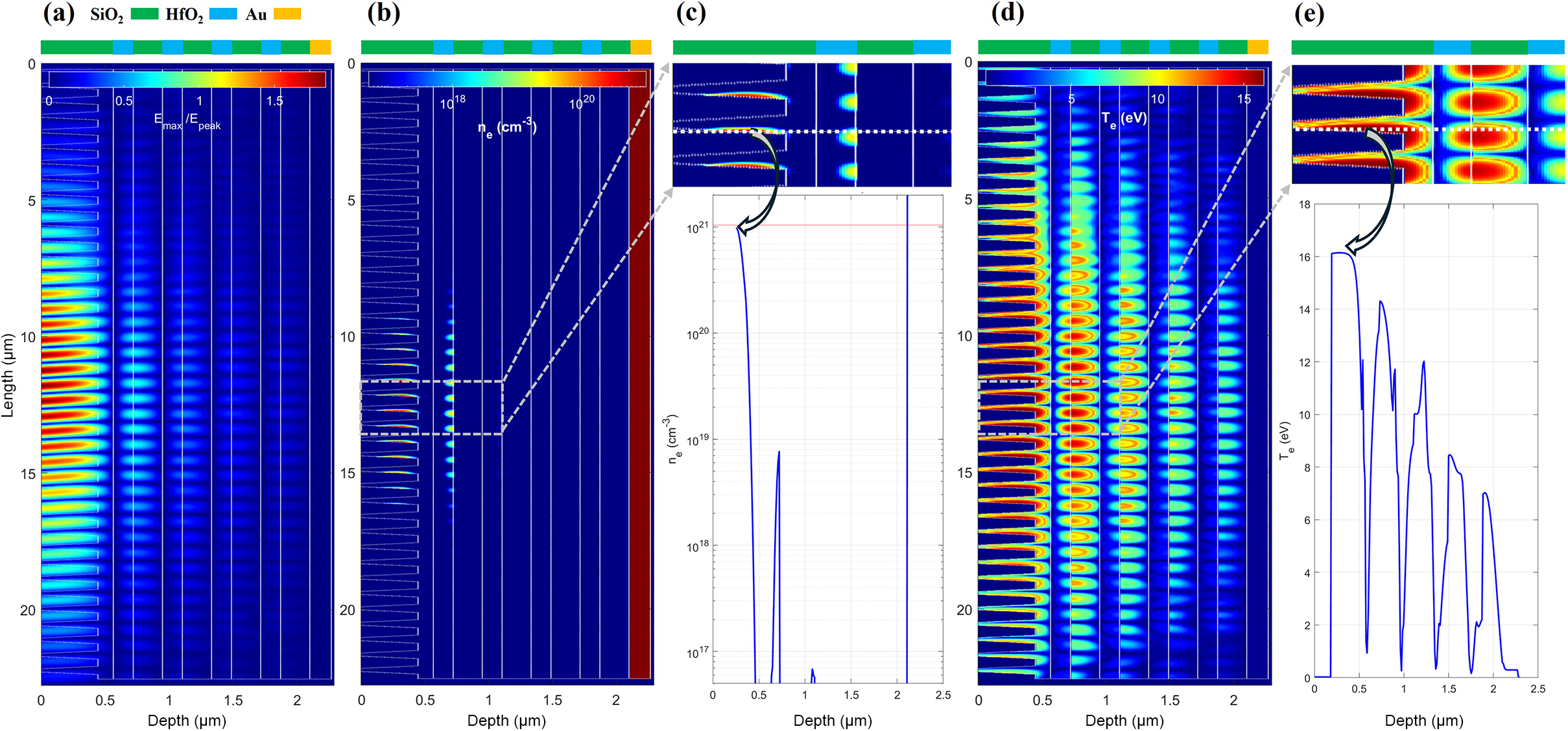
 , Figure 4(a) shows the normalized accumulated electric field enhancement, where the strongest enhancement is primarily confined to the groove regions in vacuum, reaching approximately
$1.84$
 times the incident pulse peak amplitude, while enhanced fields within the SiO
${}_2$
 pillars reach about
$1.34$
 . These values are consistent with previous simulations by Néauport et al.
[
Reference Néauport, Bonod, Hocquet, Palmier, Lavastre, Baclet and Dupuy
69
], who reported peak enhancements of
$1.87$
 in vacuum and
$1.26$
 along the pillar sidewalls. The local peak field enhancement is concentrated at the interfaces between the HfO
${}_2$
 and SiO
${}_2$
 layers, with amplitudes that remain below the incident peak field and decrease systematically with depth, from approximately
$0.76$
 at the uppermost interface to
$0.47$
 ,
$0.30$
 and
$0.19$
 at successively deeper interfaces. At the Au interface, the accumulated electric field is suppressed by approximately five orders of magnitude relative to the incident peak amplitude, indicating negligible energy penetration into the metallic layer.
Electromagnetic and carrier dynamics in the grating. (a) Accumulated peak electric field enhancement distribution within the grating. (b) Electron density distribution in the grating at
$1.1~\mathrm{ps}$
 . (c) Top: zoomed-in view of the central region of three grating pillars highlighting the global peak electron density. Bottom: 1D electron density profile extracted across the peak-density location indicated by the dashed line in the top panel. (d) Electron temperature distribution in the grating at
$1.1~\mathrm{ps}$
 . (e) Top: zoomed-in view of the central pillar region for the electron temperature. Bottom: corresponding 1D electron temperature profile extracted along the dashed line.

Figure 4 Long description
A multi-panel figure with five sections labeled a through e. At the top, a material legend identifies S i O sub 2 as grey, H f O sub 2 as green, and A u as blue and yellow.
Panel a: A heatmap of electric field enhancement E sub max all over E sub peak. The y-axis is Length from 0 to 20 micrometers and the x-axis is Depth from 0 to 2.5 micrometers. High intensity red and yellow regions are concentrated at the grating interface near 0.5 micrometers depth.
Panel b: A heatmap of electron density n sub e in units of inverse cubic centimeters. The scale ranges from 10 super 18 to 10 super 20. A dashed box highlights a central region of interest.
Panel c: Top shows a zoomed-in view of the dashed box from panel b, focusing on three grating pillars. A horizontal dashed line indicates the extraction path for the bottom graph. Bottom is a 1 D line profile of n sub e versus Depth. The density peaks sharply at approximately 10 super 21 inverse cubic centimeters at a depth of 0.4 micrometers before dropping off.
Panel d: A heatmap of electron temperature T sub e in electron volts e V, ranging from 0 to 15. The distribution shows periodic vertical bands of high temperature corresponding to the grating structure.
Panel e: Top shows a zoomed-in view of the electron temperature in the central pillars. Bottom is a 1 D line profile of T sub e versus Depth. The temperature reaches a plateau of 16 e V between 0.2 and 0.4 micrometers depth, followed by a series of decreasing peaks as depth increases toward 2.5 micrometers.
The corresponding electron density distribution is shown in Figure 4(b). Although HfO
${}_2$
 has a smaller band gap and is therefore more readily excited than SiO
${}_2$
 under the same local field enhancement, the SiO
${}_2$
 pillars at the surface experience approximately twice the electric field amplitude compared to the first HfO
${}_2$
 /SiO
${}_2$
 interface. In addition, the relatively large angle of incidence promotes multiple reflections between adjacent pillars, further enhancing the local electric field in the near-surface regions. As a result, the global peak electron density is found at the sidewalls of the top SiO
${}_2$
 pillars, where the strongest field enhancement occurs, rather than at the underlying HfO
${}_2$
 interfaces. In these regions, the electron density approaches the critical plasma density, as shown in Figure 4(c), whereas the deeper layers exhibit substantially weaker carrier generation, with the electron density in the first HfO
${}_2$
 layer being approximately two orders of magnitude lower.
The electron temperature distribution, shown in Figure 4(d), closely follows the spatial pattern of the electric field enhancement, with the highest
${T}_{\mathrm{e}}$
 reaching approximately
$16~\mathrm{eV}$
 in Figure 4(e) and confined to the same sidewall hot spots of the surface SiO
${}_2$
 pillars. In contrast to the electron density distribution, local hot spots in the deeper layers are predominantly located within the SiO
${}_2$
 regions rather than the adjacent HfO
${}_2$
 layers, which can be attributed to the lower refractive index of SiO
${}_2$
 compared to HfO
${}_2$
 , allowing stronger electric field penetration and enhancement within the material and consequently increased Ohmic heating. Deeper toward the Au layer, the peak electron temperature at the interface of Au is significantly reduced to approximately
$0.60\kern0.22em \mathrm{eV}$
 , corresponding to about
$7000\kern0.22em \mathrm{K}$
 . Based on previous studies[
Reference Chen, Tzou and Beraun
81
] reporting peak electron temperatures of the order of
$8000\kern0.22em \mathrm{K}$
 , where subsequent TTM calculations showed that the corresponding lattice temperature remained at about
$500\kern0.22em \mathrm{K}$
 , we expect that the lattice temperature in the present case likewise remains at about
$500\kern0.22em \mathrm{K}$
 as we have a longer pulse, but it still should be much lower than the melting point. Therefore, at the lower fluences, the damage initiation in this grating design is confined to the front dielectric surface rather than the underlying metal layer, which is consistent with the experiments[
Reference Néauport, Bonod, Hocquet, Palmier, Lavastre, Baclet and Dupuy
69
].
5.2 Electron density and energy evolution
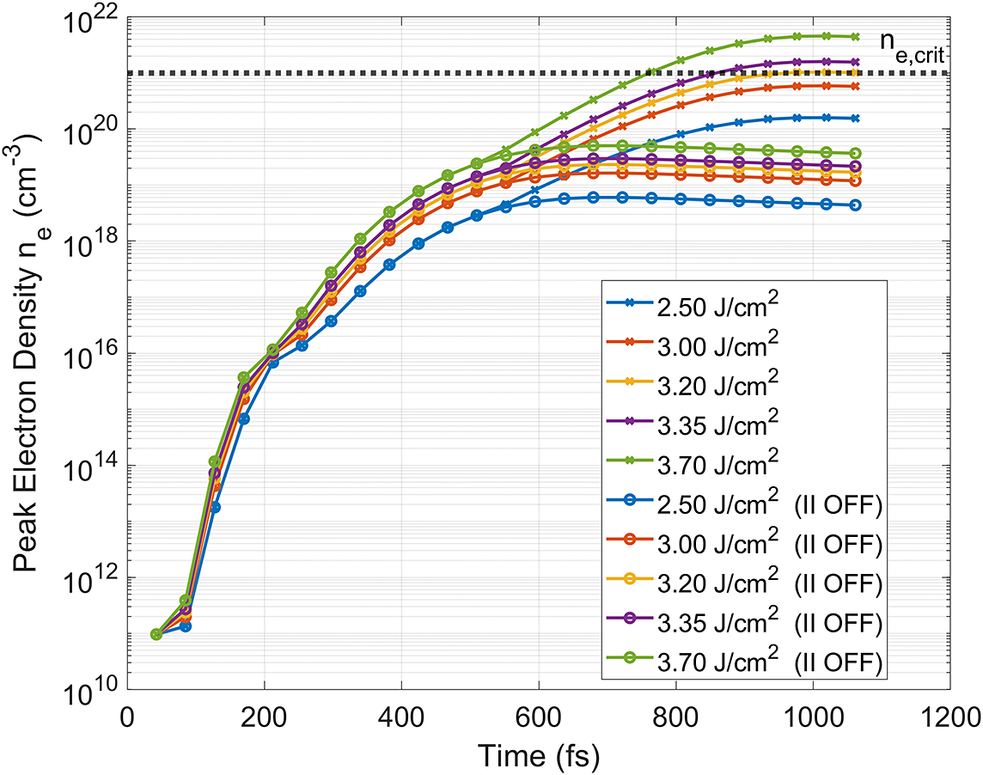
Figure 5 shows the temporal evolution of the peak electron density at different fluences, comparing simulations with II enabled and disabled over a total duration of
$1.1\;\mathrm{ps}$
 . In all cases, the electron density initially grows in a similar manner during the early stage of the interaction, dominated by PI processes. II becomes significant at approximately
$550\;\mathrm{fs}$
 , corresponding to the later half of the simulation, after which a clear divergence between the two cases is observed. By the end of the simulation, the peak electron density in the II-on cases exceeds that of the corresponding II-off cases by up to nearly two orders of magnitude, highlighting the critical role of II in carrier multiplication and plasma growth under high-fluence, ps-scale excitation. At a fluence of
$3.2\;\mathrm{J}/{\mathrm{cm}}^2$
 , the peak electron density reaches the critical plasma density, indicating the onset of laser-induced damage.
Temporal evolution of the peak electron density in the top SiO
${}_2$
 grating pillar up to
$1.06~\mathrm{ps}$
 at different fluences ranging from
$2.5$
 to
$3.7~\mathrm{J}/{\mathrm{cm}}^2$
 , comparing simulations with impact ionization enabled and disabled, with the dashed line indicating the critical plasma density.

Figure 5 Long description
A line graph with a logarithmic Y axis representing Peak Electron Density n sub e in units of c m super minus 3, ranging from 10 super 10 to 10 super 22. The X axis represents Time in f s, ranging from 0 to 1200. A horizontal dashed line near the top is labeled n sub e comma crit.
Data trends:
* All curves begin at approximately 10 super 11 c m super minus 3 at 50 f s and show a steep exponential increase until 200 f s.
* Impact Ionization Enabled (marked with x symbols): These curves continue to rise, with higher fluences reaching higher plateaus. The 3.70 J / c m super 2 and 3.35 J / c m super 2 curves cross above the critical density line between 700 and 800 f s, peaking near 10 super 21. Lower fluences (2.50 to 3.20 J / c m super 2) plateau below the critical line.
* Impact Ionization Disabled (labeled I I O F F with open circles): These curves diverge from the enabled set around 400 to 600 f s, reaching significantly lower plateaus between 10 super 18 and 10 super 20 c m super minus 3.
* The legend in the bottom right quadrant lists fluences of 2.50, 3.00, 3.20, 3.35, and 3.70 J / c m super 2 for both simulation modes.
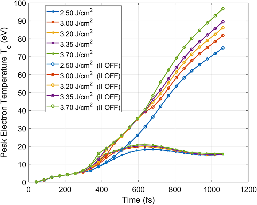
The temporal evolution of the peak electron temperature is shown in Figure 6. Before approximately
$300\;\mathrm{fs}$
 , all cases exhibit nearly identical electron temperature evolution, indicating that early-time heating is dominated by direct laser energy absorption associated with PI under relatively low instantaneous intensities. Between approximately
$450$
 and
$600\;\mathrm{fs}$
 , the II-off cases remain closely clustered, as electron heating is governed by the balance between continued laser energy deposition and limited carrier generation; consistent with Figure 5, the electron densities in the II-on and -off cases remain comparable during this interval, resulting in similar electron heat capacities and temperature rises. After approximately
$600\;\mathrm{fs}$
 , the II-off cases begin to diverge, reflecting increased sensitivity to fluence as continued energy deposition leads to progressively higher electron temperatures in the absence of efficient carrier multiplication. In contrast, when II is included, the electron temperature saturates at approximately
$20\;\mathrm{eV}$
 for all fluences, as II efficiently converts electron kinetic energy into additional carriers, increasing the electron density and electron heat capacity and thereby limiting further temperature rise. As a result, while the II-off cases continue to increase and reach peak electron temperatures approaching
$100\;\mathrm{eV}$
 , the II-on cases exhibit a pronounced temperature clamping behavior, underscoring the critical role of II in regulating electron heating during excitation processes.
Temporal evolution of the peak electron temperature in the top SiO
${}_2$
 grating pillar up to
$1.06~\mathrm{ps}$
 at different fluences ranging from
$2.5$
 to
$3.7~\mathrm{J}/{\mathrm{cm}}^2$
 , comparing simulations with impact ionization enabled and disabled.

Figure 6 Long description
The x-axis represents Time in f s from 0 to 1200. The y-axis represents Peak Electron Temperature T sub e in e V from 0 to 100.
Two distinct sets of data curves are shown for fluences of 2.50, 3.00, 3.20, 3.35, and 3.70 J per cm squared.
1. Impact Ionization Enabled (marked with crosses): All curves initially rise together until approximately 400 f s. They peak between 15 and 20 e V around 600 to 700 f s and then show a slight decline or plateau toward 1100 f s. Higher fluences result in slightly higher peak temperatures within this narrow band.
2. Impact Ionization Disabled (marked with circles and labeled I I O F F): These curves follow the same initial path until 400 f s but then diverge sharply upward. They exhibit a continuous, near-linear increase throughout the remainder of the time scale. At 1060 f s, the temperatures range from approximately 75 e V for the 2.50 J per cm squared fluence to nearly 100 e V for the 3.70 J per cm squared fluence.
The legend is located in the top-left quadrant, mapping colors and markers to the specific fluence levels and I I O F F status.
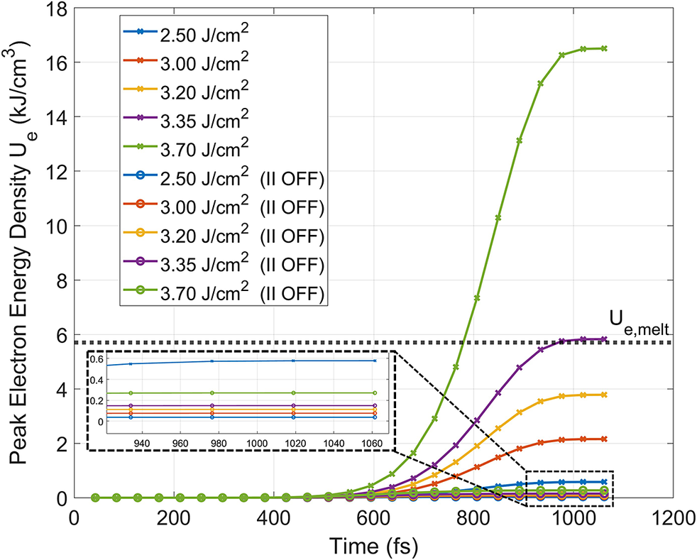
In Figure 7, the temporal evolution of the peak electron-energy density is obtained by first converting the electron temperature into kinetic energy under the ideal gas approximation, as given by Equation (24), and then multiplying by the corresponding electron density. Following the approach of Smith et al.
[
Reference Smith, Su, Zhang, Varin, Gruzdev and Chowdhury
37
], we adopt a melting energy density criterion to evaluate the LIDT, which has been shown to provide good predictive capability for ultrafast laser damage. Using thermophysical data from Zhao et al.
[
Reference Zhao, Sullivan, Zayac and Bennett
82
,
Reference Zhao, Cheng, Chen, Yuan, Liao, Wang, Liu and Yang
83
], the melting energy density of the dielectric material is calculated to be approximately
$5.7\;\mathrm{kJ}/{\mathrm{cm}}^3$
 . Although the II-off cases exhibit substantially higher peak electron temperatures, the associated electron densities remain relatively low, resulting in significantly reduced electron-energy densities compared to the II-on cases. As a consequence, only simulations including II are able to accumulate sufficient energy density to approach the melting threshold. At a fluence of
$3.35\;\mathrm{J}/{\mathrm{cm}}^2$
 , the peak electron-energy density reaches the calculated melting energy density, indicating the onset of laser-induced damage according to the energy-density-based criterion.
Temporal evolution of the peak electron-energy density in the top SiO
${}_2$
 grating pillar up to
$1.06~\mathrm{ps}$
 at fluences ranging from
$2.5$
 to
$3.7~\mathrm{J}/{\mathrm{cm}}^2$
 , comparing simulations with impact ionization enabled and disabled, with the dashed line indicating the melting energy density; the inset shows a zoomed-in view of the II-off cases, which terminate at approximately
$0.05$
 –
$0.60~\mathrm{kJ}/{\mathrm{cm}}^3$
 by the end of the simulation.

Figure 7 Long description
A line graph plots Peak Electron Energy Density U sub e in k J per c m cubed on the y-axis against Time in f s on the x-axis. The x-axis ranges from 0 to 1200 and the y-axis from 0 to 18.
Ten data series are shown, representing fluences of 2.50, 3.00, 3.20, 3.35, and 3.70 J per c m squared. Each fluence has two versions: one with impact ionization enabled (marked with crosses) and one labeled I I O F F (marked with open circles).
Data Trends:
- For all fluences, energy density remains near zero until approximately 500 f s.
- Cases with impact ionization enabled show a rapid sigmoidal increase. The 3.70 J per c m squared curve rises most sharply, peaking at approximately 16.5 k J per c m cubed. The 3.35 J per c m squared curve plateaus near 6 k J per c m cubed.
- A horizontal dashed line labeled U sub e comma melt is positioned at approximately 5.7 k J per c m cubed, indicating the melting threshold.
- All I I O F F cases remain extremely low, appearing as flat lines near the bottom of the main plot.
Inset Details:
- An inset in the bottom left zooms into the time range 920 to 1060 f s and y-axis range 0 to 0.6.
- It reveals that the I I O F F curves are not perfectly flat but show very slight linear increases, with the 3.70 J per c m squared I I O F F case reaching approximately 0.6 k J per c m cubed by the end of the simulation.
5.3 Laser-induced damage threshold
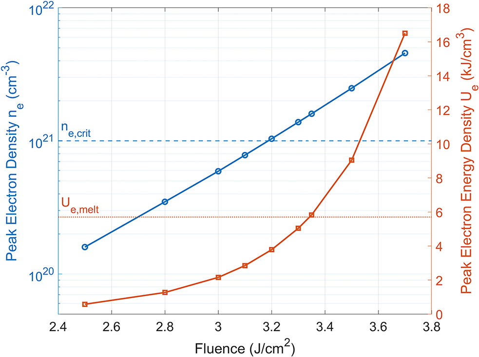
Finally, Figure 8 summarizes the predicted LIDT based on two criteria, namely the critical plasma density and the melting energy density, over the tested range from
$2.5$
 to
$3.7\;\mathrm{J}/{\mathrm{cm}}^2$
 . Using the critical density criterion, the onset of damage is predicted at a fluence of approximately
$3.2\;\mathrm{J}/{\mathrm{cm}}^2$
 , whereas the melting energy density criterion yields a slightly higher threshold of about
$3.35\;\mathrm{J}/{\mathrm{cm}}^2$
 . These predictions are in reasonable agreement with the experimentally measured
$100$
 -on-
$1$
 damage threshold of approximately
$3.24\;\mathrm{J}/{\mathrm{cm}}^2$
 . Uncertainty values are not reported in the original work. However, based on the measurement procedure described in earlier work[
Reference Neauport, Lavastre, Razé, Dupuy, Bonod, Balas, de Villele, Flamand, Kaladgew and Desserouer
84
], the uncertainty is approximately
$2\%$
 for a single site, with LIDT variations up to approximately
$10\%$
 across testing at different locations. Although initially it appears to be an ‘apples (simulation LIDT for single-shot damage initiation) to oranges (exp LIDT for 100-on-1 shots, significant damage and ablation)’ comparison, the 100-on-1 heavy damage/ablation threshold fluence most likely is near the single-shot damage initiation threshold, which the simulation predicts. Despite this difference in damage manifestation, the close agreement between the predicted thresholds and the experimental result suggests that the present modeling framework provides a reliable estimate of the LIDT for the hybrid coatings. Between the two criteria, the critical electron density criterion shows slightly better agreement with the experimentally determined threshold, consistent with its typical applicability to longer pulse durations.
LIDT predicted using the critical electron density and melting electron-energy density criteria over a tested fluence range of
$2.5$
 –
$3.7~\mathrm{J}/{\mathrm{cm}}^2$
 , with the critical density threshold indicated at
$3.2~\mathrm{J}/{\mathrm{cm}}^2$
 by the blue dashed line and the melting energy density threshold predicted at
$3.35~\mathrm{J}/{\mathrm{cm}}^2$
 .

Figure 8 Long description
A dual-axis line graph. The horizontal X-axis represents Fluence in J / cm super 2, ranging from 2.4 to 3.8. The left Y-axis, in blue, represents Peak Electron Density n sub e in cm super -3 on a logarithmic scale from 10 super 20 to 10 super 22. The right Y-axis, in orange, represents Peak Electron Energy Density U sub e in k J / cm super 3 on a linear scale from 0 to 18.
* The blue data series with circular markers shows a steady logarithmic increase in peak electron density as fluence increases, crossing the 10 super 21 mark at approximately 3.2 J / cm super 2.
* The orange data series with square markers shows an exponential increase in peak electron energy density, starting near 1 k J / cm super 3 at 2.5 J / cm super 2 and rising sharply to over 16 k J / cm super 3 at 3.7 J / cm super 2.
* A horizontal blue dashed line labeled n sub e,crit is positioned at 10 super 21 on the left axis.
* A horizontal orange dotted line labeled U sub e,melt is positioned at approximately 5.8 on the right axis, intersecting the orange data curve at a fluence of 3.35 J / cm super 2.
6 Conclusion
In conclusion, we have developed a multiscale modeling framework to investigate sub-ps laser interaction and damage initiation in multilayer hybrid coatings. The framework captures nonlinear near-field enhancement and resolves the spatiotemporal evolution of electron density, electron temperature and electron-energy density under the assumption of rapid electron thermalization, showing good agreement with experimental results. In addition, the approach provides a useful capability to compare different laser-induced damage criteria against experimental observations and evaluate their applicability for predicting the LIDT. Our results provide valuable guidance for the design of optical coatings in high-power laser systems and illustrate the complex physical mechanisms governing laser–matter interactions in the 10 fs to 1 ps regime.
Future extensions of this work will use the electron temperature obtained from the present simulations as initial conditions for TTM calculations, enabling the description of longer-time electron–lattice energy relaxation, particularly within the metal region. In addition, extending the present framework to full three-dimensional implementations will enable complex meta-surface modeling, with broader applications in high-power laser systems, beam control and laser-driven fusion technologies.
Acknowledgements
This work was partially supported by the DOE STTR (Award No. DE-SC0019900) and AFOSR (No. FA9550-25-1-0297) and used resources from the Ohio Supercomputer Center.












 Open access

