



1 Introduction
Buoyant interpenetrating flows, due to the release of a heavy mixture into a light one, are amongst the most fundamental fluid mechanics problems widely found in nature within oceanographic, meteorological and geophysical contexts (Benjamin Reference Benjamin1968; Shin, Dalziel & Linden Reference Shin, Dalziel and Linden2004; Birman et al. Reference Birman, Battandier, Meiburg and Linden2007). They also have numerous applications in industry, such as in continuous reactors and countercurrent extraction columns (Pratt & Baird Reference Pratt, Baird, Lo, Baird and Hanson1983; Baird et al. Reference Baird, Aravamudan, Rao, Chadam and Peirce1992). These multiphase flows have been widely studied in the literature, experimentally by Debacq et al. (Reference Debacq, Fanguet, Hulin, Salin and Perrin2001), Seon et al. (Reference Seon, Hulin, Salin, Perrin and Hinch2005, Reference Seon, Znaien, Salin, Hulin, Hinch and Perrin2007a ), Znaien, Moisy & Hulin (Reference Znaien, Moisy and Hulin2011) and Alba, Taghavi & Frigaard (Reference Alba, Taghavi and Frigaard2012, Reference Alba, Taghavi and Frigaard2013a ), computationally by Sahu & Vanka (Reference Sahu and Vanka2011), Taghavi, Alba & Frigaard (Reference Taghavi, Alba and Frigaard2012a ), Alba, Taghavi & Frigaard (Reference Alba, Taghavi and Frigaard2014), Hallez & Magnaudet (Reference Hallez and Magnaudet2015) and Sebilleau, Issa & Walker (Reference Sebilleau, Issa and Walker2016) and analytically by Seon et al. (Reference Seon, Znaien, Salin, Hulin, Hinch and Perrin2007b ), Taghavi et al. (Reference Taghavi, Seon, Martinez and Frigaard2009, Reference Taghavi, Alba, Seon, Wielage-Burchard, Martinez and Frigaard2012b ), Kerswell (Reference Kerswell2011), Borden & Meiburg (Reference Borden and Meiburg2013) and Alba, Taghavi & Frigaard (Reference Alba, Taghavi and Frigaard2013b ), considering a pair of pure fluids. Depending on the flow configuration and parameters, various viscous, transitionary and diffusive regimes, governed by the balance of viscous, buoyant and inertial forces, may emerge, as laid out by Seon et al. (Reference Seon, Hulin, Salin, Perrin and Hinch2006), Sahu & Vanka (Reference Sahu and Vanka2011) and Alba et al. (Reference Alba, Taghavi and Frigaard2013a ). In many practical situations, however, the involved fluids are particle-laden (suspension) and therefore not pure. Particle-laden flows have been studied in the literature only in the context of Boycott flow (settlement-induced convection within a single suspension mixture) by Boycott (Reference Boycott1920) and Davis, Herbolzheimer & Acrivos (Reference Davis, Herbolzheimer and Acrivos1983), turbidity currents (intrusion of a suspension into a liquid ambient over a nearly horizontal free-surface geometry) by Bonnecaze, Huppert & Lister (Reference Bonnecaze, Huppert and Lister1993) and Meiburg & Kneller (Reference Meiburg and Kneller2010), and debris flows (intrusion of a suspension into a gas ambient over an incline) by Cook (Reference Cook2008), Cook, Bertozzi & Hosoi (Reference Cook, Bertozzi and Hosoi2008) and Wang et al. (Reference Wang, Mavromoustaki, Bertozzi, Urdaneta and Huang2015). The interpenetrating exchange flow of a suspension into another fluid in a practical duct geometry has received very little attention in the literature due to the increased complexity arising from the interaction of the solid–fluid as well as fluid–fluid phases within enclosed walls. One of the few studies available in the literature on this topic is the recent work of Saha, Salin & Talon (Reference Saha, Salin and Talon2013) carried out experimentally for a horizontal configuration. Numerous applications of particle-laden interpenetrating flows are found in a variety of industrial operations, such as discharge, transport and dispersion of slurries, mine tailings, pastes, pharmaceuticals, paper pulp, drill cuttings, sludge, effluents and sewage, also the manufacture of cement clinker in inclined kilns, mineral processing in hydrocyclones, and fluidized beds, as discussed by Segre & Silberberg (Reference Segre and Silberberg1961), Asomah & Napier-Munn (Reference Asomah and Napier-Munn1997), Hamed (Reference Hamed2005), Nelson & Guillot (Reference Nelson and Guillot2006), Wiklund et al. (Reference Wiklund, Stading, Pettersson and Rasmuson2006) and Boateng (Reference Boateng2015).
The lubrication approximation can be applied to model flows in the buoyant viscous domain with negligible inertia. A continuum one-dimensional lubrication model of a particle-laden film flowing down a slope was first developed by Zhou et al. (Reference Zhou, Dupuy, Bertozzi and Hosoi2005), predicting the evolution of the interface height,
 $h$
, and particle volume fraction,
 $\unicode[STIX]{x1D719}$
, with time,
 $t$
, and streamwise distance,
 $x$
. Zhou et al. (Reference Zhou, Dupuy, Bertozzi and Hosoi2005), Cook (Reference Cook2008) and Cook et al. (Reference Cook, Bertozzi and Hosoi2008) reported the formation of a particle-rich ridge in the vicinity of the advancing suspension front (contact line) due to the different rates of solid and fluid transport. Two-dimensional (2D) effects were later studied by Cook, Alexandrov & Bertozzi (Reference Cook, Alexandrov and Bertozzi2009), revealing that the addition of solid particles can diminish the well-known fingering instabilities of an advancing contact line. While there is a large body of studies on modelling single-layer suspension film flows, the literature on two-layer exchange systems of suspension and pure fluid is severely lacking. As a novel approach, we extend the methodology of Zhou et al. (Reference Zhou, Dupuy, Bertozzi and Hosoi2005) for free-surface film flows to a practical exchange system within a confined (duct) geometry. As discussed by Kerswell (Reference Kerswell2011), the exchange flow of two fluids in a vertical duct may reveal slumping side-by-side or symmetric patterns with either heavy or light fluids moving in the core region of the duct. In particular, we are interested in the symmetric mode where the heavy particle-laden film falls along the side walls and the light fluid moves upwards in the centre of the duct; see figure 1. From a different perspective, the examined exchange flow can be considered as an extension to the fundamental Taylor bubble problem of Davies & Taylor (Reference Davies and Taylor1950), now studied for particle-laden fluids.
Schematic of the symmetric particle-laden exchange flow in a vertical 2D duct used in the lubrication model analysis. Note that dimensional notations are used in the figure. The interface shape is illustrative only.
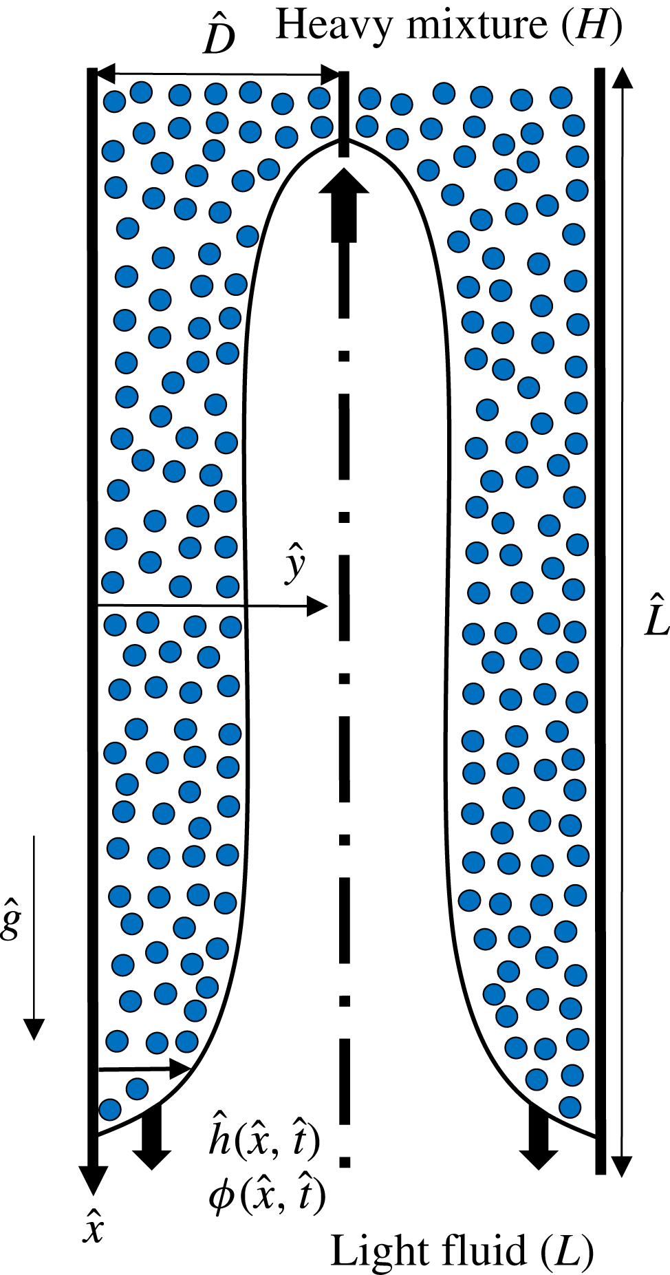
The important dimensional and dimensionless parameters of the problem are first laid out in § 2. The lubrication model is then derived in § 3. A total variation diminishing (TVD) finite difference scheme, used to numerically solve the derived model, is explained in § 4. In the presentation of our results in § 5, we first discuss the case of pure fluids and then examine the effect of particle addition to the flow. The effects of a wide range of controlling parameters, such as the density, size and volume fraction of particles, as well as the viscosity and density of the light and carrying fluids, and the Reynolds number, are investigated in detail. The paper closes with a brief summary in § 6. A last note here is that the model developed in this paper is unable to capture interfacial instabilities due to the inherent lubrication model assumption used (negligible inertia). This model is only applicable to highly viscous regimes with negligible inertia (Taghavi et al. Reference Taghavi, Seon, Martinez and Frigaard2009). The authors have extensively studied the stability of thin pure fluid films in their previous works, such as in Alba, Laure & Khayat (Reference Alba, Laure and Khayat2011), Taghavi et al. (Reference Taghavi, Alba, Seon, Wielage-Burchard, Martinez and Frigaard2012b ) and Alba et al. (Reference Alba, Taghavi and Frigaard2013b ), via a weighted residual (WR) model. Extending the current particle-laden formulation to a similar WR model, capable of capturing instabilities, is extremely challenging due to the addition of weakly inertial terms in the Navier–Stokes equations.
2 Dimensional and dimensionless governing parameters
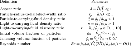
The problem shown schematically in figure 1 involves 11 dimensional parameters, which we denote with the
 $\hat{~}$
symbol. The gravitational acceleration is denoted by
 ${\hat{g}}$
. The vertical duct has width,
 $2\hat{D}$
, and length,
 $\hat{L}$
. The duct geometry considered may simulate particle-laden groundwater flows through aquifers, conduits, caves, cracks, joints and faults. To capture the fully developed flow effects as discussed by Alba et al. (Reference Alba, Taghavi and Frigaard2013a
), we assume
 $\hat{L}\gg \hat{D}$
. The solid particles, which are considered to be heavier than the carrying fluid (negatively buoyant), have radius
 $\hat{a}$
and density
 $\hat{\unicode[STIX]{x1D70C}}_{p}$
. In particular, we are interested in non-Brownian suspensions, i.e.
 $\hat{a}>1~\unicode[STIX]{x03BC}\text{m}$
(Espín & Kumar Reference Espín and Kumar2014). The Newtonian carrying fluid in the heavy solution has density
 $\hat{\unicode[STIX]{x1D70C}}_{f,H}$
and viscosity
 $\hat{\unicode[STIX]{x1D707}}_{f,H}$
. Similarly, the Newtonian light fluid density and viscosity are denoted by
 $\hat{\unicode[STIX]{x1D70C}}_{L}$
and
 $\hat{\unicode[STIX]{x1D707}}_{L}$
, respectively. Both the fluids and solid phases are assumed to be incompressible. The initial total volume of particles is
 $\hat{V}_{p}$
. At time
 $\hat{t}=0~\text{s}$
, the heavy particle-laden mixture occupies the top half of the duct (
 $\hat{x}<0$
) whereas the light pure fluid takes up the bottom half (
 $\hat{x}\geqslant 0$
). The jamming volume, which depends on the shape and packing arrangement of the particles, is further designated by
 $\hat{V}_{j}$
(Saha et al.
Reference Saha, Salin and Talon2013). Through a dimensional analysis based on Buckingham’s
 $\unicode[STIX]{x03C0}$
theorem, it is not difficult to show that eight dimensionless parameters control the flow in question, namely the duct aspect ratio,
 $\unicode[STIX]{x1D6FF}=\hat{D}/\hat{L}\ll 1$
, particle-radius-to-half-duct-width ratio,
 $r_{p}=\hat{a}/\hat{D}$
, particle-to-carrying-fluid density ratio,
 $\unicode[STIX]{x1D709}=\hat{\unicode[STIX]{x1D70C}}_{p}/\hat{\unicode[STIX]{x1D70C}}_{f,H}$
, light-to-carrying-fluid density ratio,
 $\unicode[STIX]{x1D702}=\hat{\unicode[STIX]{x1D70C}}_{L}/\hat{\unicode[STIX]{x1D70C}}_{f,H}$
, light-to-carrying-fluid viscosity ratio,
 $\unicode[STIX]{x1D705}=\hat{\unicode[STIX]{x1D707}}_{L}/\hat{\unicode[STIX]{x1D707}}_{f,H}$
, initial volume fraction of particles,
 $\unicode[STIX]{x1D719}_{0}=\hat{V}_{p}/\hat{V}_{H}$
, jamming volume fraction,
 $\unicode[STIX]{x1D719}_{j}=\hat{V}_{j}/\hat{V}_{H}$
, and the Reynolds number,
 $Re=\hat{\unicode[STIX]{x1D70C}}_{H}(\unicode[STIX]{x1D719}_{0})\hat{V}_{t}(2\hat{D})/\hat{\unicode[STIX]{x1D707}}_{H}(\unicode[STIX]{x1D719}_{0})$
. Similar to the approach of Cook et al. (Reference Cook, Bertozzi and Hosoi2008), we assume that the volume fraction of particles across the depth of the suspension layer,
 $y$
, is uniform, i.e.
 $\unicode[STIX]{x1D719}=\unicode[STIX]{x1D719}(x,t)$
only. See Metzger, Guazzelli & Butler (Reference Metzger, Guazzelli and Butler2005) for particle heterogeneity effects in sedimentary flows and appendix A for negligibility of shear-induced migration effects. Assuming that the duct has unit depth, the total volume of the heavy solution is found as
 $\hat{V}_{H}=\hat{D}\hat{L}$
. Further assuming monodisperse spherical particles, the jamming volume fraction is obtained as
 $\unicode[STIX]{x1D719}_{j}\approx 0.67$
(Cook et al.
Reference Cook, Bertozzi and Hosoi2008). The expressions
 $\hat{\unicode[STIX]{x1D70C}}_{H}(\unicode[STIX]{x1D719}_{0})=\hat{\unicode[STIX]{x1D70C}}_{p}\unicode[STIX]{x1D719}_{0}+\hat{\unicode[STIX]{x1D70C}}_{f,H}(1-\unicode[STIX]{x1D719}_{0})$
and
 $\hat{\unicode[STIX]{x1D707}}_{H}(\unicode[STIX]{x1D719}_{0})=\hat{\unicode[STIX]{x1D707}}_{f,H}(1-\unicode[STIX]{x1D719}_{0}/\unicode[STIX]{x1D719}_{j})^{-2}$
determine the density and viscosity of the heavy fluid, respectively (Saha et al.
Reference Saha, Salin and Talon2013). The characteristic velocity in the Reynolds-number expression is defined as
 $\hat{V}_{t}=\sqrt{(1-\unicode[STIX]{x1D713}){\hat{g}}\hat{D}/(1+\unicode[STIX]{x1D713})}$
, where
 $\unicode[STIX]{x1D713}=\hat{\unicode[STIX]{x1D70C}}_{L}/\hat{\unicode[STIX]{x1D70C}}_{H}(\unicode[STIX]{x1D719}_{0})=\unicode[STIX]{x1D702}/(1+(\unicode[STIX]{x1D709}-1)\unicode[STIX]{x1D719}_{0})$
is the density ratio of the light fluid to the heavy suspension. In our simulations,
 $\unicode[STIX]{x1D702}$
can be larger than
 $1$
, i.e. the light fluid heavier than the carrying fluid. However,
 $\unicode[STIX]{x1D713}$
is always less than
 $1$
, meaning that the overall suspension mixture is heavier than the light fluid. The dimensional parameters governing the flow along with the dimensionless numbers and their ranges are listed in tables 1 and 2.
List of dimensional independent input parameters of the problem.

List of dimensionless independent input parameters of the problem.
3 Lubrication model derivation
We aim to construct a lubrication model in simplified vertical 2D channel geometry, shown schematically in figure 1. Owing to symmetry, only half of the duct domain between the left wall (
 $y=0$
) and centre (
 $y=1$
) is considered in the model. Extending the model to a pipe geometry, potentially more convenient for experimentation, is performed in appendix B. As discussed in depth in appendix A, for the Boussinesq limit considered (
 $At\ll 1$
where
 $At=(\hat{\unicode[STIX]{x1D70C}}_{H}(\unicode[STIX]{x1D719}_{0})-\hat{\unicode[STIX]{x1D70C}}_{L})/(\hat{\unicode[STIX]{x1D70C}}_{H}(\unicode[STIX]{x1D719}_{0})+\hat{\unicode[STIX]{x1D70C}}_{L})=(1-\unicode[STIX]{x1D713})/(1+\unicode[STIX]{x1D713})$
is the Atwood number), we may neglect the diffusive effects associated with shear-induced migration of particles (Cook et al.
Reference Cook, Bertozzi and Hosoi2008; Mavromoustaki & Bertozzi Reference Mavromoustaki and Bertozzi2014; Wang & Bertozzi Reference Wang and Bertozzi2014). A lubrication model describing viscous exchange flow of pure fluids has been developed in our recent work (Hasnain & Alba Reference Hasnain and Alba2017) for which the configuration was considered to be slumping, i.e. no-slip condition at both
 $y=0$
and
 $1$
. Here, we adopt a symmetric configuration, i.e. no-slip condition at
 $y=0$
and stress-free condition at
 $y=1$
. Following the approach of Hasnain & Alba (Reference Hasnain and Alba2017), the governing streamwise and depthwise momentum equations in the heavy particle-laden layer reduce to
 $$\begin{eqnarray}\displaystyle & \displaystyle 0=-p_{x}+{\displaystyle \frac{\unicode[STIX]{x1D70C}_{H}(\unicode[STIX]{x1D719})Re}{1-\unicode[STIX]{x1D713}}}+\unicode[STIX]{x1D707}_{H}(\unicode[STIX]{x1D719})u_{yy}, & \displaystyle\end{eqnarray}$$
 $$\begin{eqnarray}\displaystyle & \displaystyle 0=-p_{y}, & \displaystyle\end{eqnarray}$$
where we have scaled the streamwise and depthwise distances by
 $\hat{D}/\unicode[STIX]{x1D6FF}$
and
 $\hat{D}$
, respectively. Moreover, the pressure has been scaled by
 $\hat{\unicode[STIX]{x1D707}}_{H}(\unicode[STIX]{x1D719}_{0})\hat{V}_{t}/\unicode[STIX]{x1D6FF}\hat{D}$
. The dimensionless density and viscosity of the heavy layer in the continuum form and as a function of the particle volume fraction,
 $\unicode[STIX]{x1D719}$
, are expressed as (Cook et al.
Reference Cook, Bertozzi and Hosoi2008)
 $$\begin{eqnarray}\displaystyle & \displaystyle \unicode[STIX]{x1D70C}_{H}(\unicode[STIX]{x1D719})={\displaystyle \frac{1+(\unicode[STIX]{x1D709}-1)\unicode[STIX]{x1D719}}{1+(\unicode[STIX]{x1D709}-1)\unicode[STIX]{x1D719}_{0}}}, & \displaystyle\end{eqnarray}$$
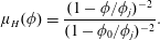 $$\begin{eqnarray}\displaystyle & \displaystyle \unicode[STIX]{x1D707}_{H}(\unicode[STIX]{x1D719})={\displaystyle \frac{(1-\unicode[STIX]{x1D719}/\unicode[STIX]{x1D719}_{j})^{-2}}{(1-\unicode[STIX]{x1D719}_{0}/\unicode[STIX]{x1D719}_{j})^{-2}}}. & \displaystyle\end{eqnarray}$$
Similarly, for the light fluid layer we obtain
 $$\begin{eqnarray}\displaystyle & \displaystyle 0=-p_{x}+{\displaystyle \frac{\unicode[STIX]{x1D713}Re}{1-\unicode[STIX]{x1D713}}}+mu_{yy}, & \displaystyle\end{eqnarray}$$
 $$\begin{eqnarray}\displaystyle & \displaystyle 0=-p_{y}, & \displaystyle\end{eqnarray}$$
where
 $m=\hat{\unicode[STIX]{x1D707}}_{L}/\hat{\unicode[STIX]{x1D707}}_{H}(\unicode[STIX]{x1D719}_{0})=\unicode[STIX]{x1D705}(1-\unicode[STIX]{x1D719}_{0}/\unicode[STIX]{x1D719}_{j})^{2}$
is the viscosity ratio of the light fluid to that of the heavy suspension layer. Integrating (3.2) and (3.6) across the width gives
 $$\begin{eqnarray}\displaystyle & \displaystyle p=p_{0}(x,t)+{\displaystyle \frac{\unicode[STIX]{x1D70C}_{H}(\unicode[STIX]{x1D719})xRe}{1-\unicode[STIX]{x1D713}}},\quad 0\leqslant y\leqslant 1, & \displaystyle\end{eqnarray}$$
where we define
 $p_{0}(x,t)$
as
 $$\begin{eqnarray}\displaystyle & \displaystyle p_{0}(x,t)=p(x,0,t)-{\displaystyle \frac{\unicode[STIX]{x1D70C}_{H}(\unicode[STIX]{x1D719})xRe}{1-\unicode[STIX]{x1D713}}}. & \displaystyle\end{eqnarray}$$
In obtaining (3.7), we neglected the effects of interfacial tension between the two mixtures for simplicity. In other words, we consider an immiscible interface but with zero interfacial tension. Such a limit is indeed equivalent to a miscible interface with zero molecular diffusion; see Petitjeans & Maxworthy (Reference Petitjeans and Maxworthy1996), Taghavi et al. (Reference Taghavi, Alba, Seon, Wielage-Burchard, Martinez and Frigaard2012b ) and Alba et al. (Reference Alba, Taghavi and Frigaard2013b ) for studies taking a similar approach for pure fluids.
The pressure expression (3.7) is now used in the streamwise momentum equations (3.1) and (3.5) to give
 $$\begin{eqnarray}\displaystyle & \displaystyle 0=-P_{0,x}+\unicode[STIX]{x1D707}_{H}(\unicode[STIX]{x1D719})u_{yy},\quad 0\leqslant y\leqslant h, & \displaystyle\end{eqnarray}$$
 $$\begin{eqnarray}\displaystyle & \displaystyle 0=-P_{0,x}-{\displaystyle \frac{\unicode[STIX]{x1D70C}_{H}(\unicode[STIX]{x1D719})-\unicode[STIX]{x1D713}}{1-\unicode[STIX]{x1D713}}}Re+mu_{yy},\quad h\leqslant y\leqslant 1. & \displaystyle\end{eqnarray}$$
Note that, for simplification, we have defined
 $P_{0,x}=p_{0,x}+(x\unicode[STIX]{x1D70C}_{H,\unicode[STIX]{x1D719}}\unicode[STIX]{x1D719}_{x}Re)/(1-\unicode[STIX]{x1D713})$
. Applying appropriate boundary and interfacial conditions in (3.11)–(3.13), the equations (3.9) and (3.10) can be integrated with respect to
 $y$
in order to determine the streamwise velocity closures in each layer. In the case of miscible fluids, a standard no-slip condition at the lower wall (
 $y=0$
) may be used. However, in the case of immiscible fluids, we face the well-known contact-line problem due to the singularity of the stress at the walls. Many authors have worked intensely for decades to address this issue, suggesting a wide range of remedies, e.g. replacing no-slip conditions at the wall by Navier slip ones (Greenspan Reference Greenspan1978), assuming a narrow precursor film of thickness
 $b$
in the vicinity of the wall as laid out by Spaid & Homsy (Reference Spaid and Homsy1996), etc. As mentioned in § 1, similar to Cook et al. (Reference Cook, Bertozzi and Hosoi2008) we are interested in a scenario where the suspension mixture flows close to the surface of the duct wall. The precursor film approach then suits our application the best. In fact, the validity of such an assumption for particle-laden flows has been confirmed in the experiments of Zhou et al. (Reference Zhou, Dupuy, Bertozzi and Hosoi2005). Owing to the symmetry, we can further apply the stress-free condition in the duct centre (
 $y=1$
). In summary, we have
 $$\begin{eqnarray}\displaystyle & \displaystyle u=0,\quad \text{at}\,y=0, & \displaystyle\end{eqnarray}$$
 $$\begin{eqnarray}\displaystyle & \displaystyle u_{y}=0,\quad \text{at}\,y=1. & \displaystyle\end{eqnarray}$$
The homogeneity of the velocity and stress at the interface,
 $h$
, requires
 $$\begin{eqnarray}\displaystyle [u]=0,\quad [\unicode[STIX]{x1D70F}_{xy}]=0,\quad \text{at}\,\,y=h, & & \displaystyle\end{eqnarray}$$
where
 $[~]$
denotes the jump of the given quantity. Note that in (3.13),
 $\unicode[STIX]{x1D70F}_{xy}=u_{y}$
for the heavy and
 $\unicode[STIX]{x1D70F}_{xy}=mu_{y}$
for the light fluids, respectively. The last condition needed to solve the system of equations (3.9) and (3.10) for the velocity closures is the total flow constraint,
 $$\begin{eqnarray}\displaystyle \int _{0}^{1}u\,\text{d}y=0. & & \displaystyle\end{eqnarray}$$
The streamwise velocity,
 $u$
, in the heavy and light layers can then be obtained by integrating (3.9) and (3.10) twice as
 $$\begin{eqnarray}\displaystyle & \displaystyle u={\displaystyle \frac{P_{0,x}y^{2}}{2\unicode[STIX]{x1D707}_{H}}}+c_{1}y+c_{2},\quad 0\leqslant y\leqslant h, & \displaystyle\end{eqnarray}$$
 $$\begin{eqnarray}\displaystyle & \displaystyle u=\left(P_{0,x}+{\displaystyle \frac{\unicode[STIX]{x1D70C}_{H}-\unicode[STIX]{x1D713}}{1-\unicode[STIX]{x1D713}}}Re\right){\displaystyle \frac{y^{2}}{2m}}+d_{1}y+d_{2},\quad h\leqslant y\leqslant 1, & \displaystyle\end{eqnarray}$$
where
 $P_{0,x}$
,
 $c_{1}$
,
 $c_{2}$
,
 $d_{1}$
and
 $d_{2}$
are coefficients given in appendix C. The flux function,
 $q=\hat{q}/\hat{D}$
, as the flow rate within the heavy layer can eventually be calculated as
 $$\begin{eqnarray}\displaystyle q=\int _{0}^{h}u\,\text{d}y, & & \displaystyle\end{eqnarray}$$
which is given in appendix D as a function of
 $h$
,
 $Re$
,
 $m$
,
 $\unicode[STIX]{x1D707}_{H}$
and
 $\unicode[STIX]{x1D70C}_{H}$
. In the case of pure fluids (
 $\unicode[STIX]{x1D719}_{0}=0$
), we obtain
 $\unicode[STIX]{x1D70C}_{H}=\unicode[STIX]{x1D707}_{H}=1$
from (3.3) and (3.4). The relevant dimensionless numbers governing the flow would then be reduced to
 $Re$
and
 $\unicode[STIX]{x1D705}$
. Note that, since
 $\unicode[STIX]{x1D70C}_{H}=1$
in (3.16), the model becomes independent of
 $\unicode[STIX]{x1D713}$
(thus
 $\unicode[STIX]{x1D702}$
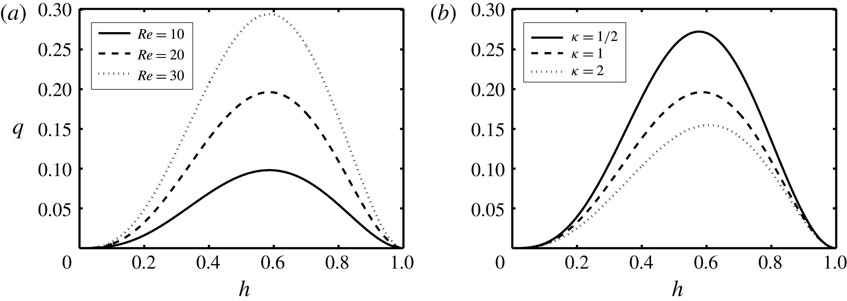
). Figures 2(a) and 2(b) show the variation of
 $q$
versus
 $h$
for different values of
 $Re$
and
 $\unicode[STIX]{x1D705}$
, respectively. As
 $h\rightarrow 0$
and
 $1$
,
 $q\rightarrow 0$
. The flux function
 $q$
exhibits a maximum in the interval
 $h\in [0,1]$
. The location of this maximum remains unchanged in the iso-viscous case,
 $h\approx 0.586$
; see figure 2(a). However, the maximal
 $q$
location shifts slightly to the left (smaller
 $h$
) with decreasing viscosity ratio,
 $\unicode[STIX]{x1D705}$
, i.e. less viscous light fluid, as shown in figure 2(b).
Variation of the flux function,
 $q$
, in (3.17) with interface height,
 $h$
, for pure fluids (
 $\unicode[STIX]{x1D719}_{0}=r_{p}=\unicode[STIX]{x1D709}=0$
) and (a)
 $\unicode[STIX]{x1D705}=1$
at various values of
 $Re$
, and (b)
 $Re=20$
at various values of
 $\unicode[STIX]{x1D705}$
. Owing to the choice of scaling used, the results in the pure fluids limit do not depend on
 $\unicode[STIX]{x1D702}$
.
The evolution equations for the interface height and particle volume fraction, respectively, read (see also Cook et al. (Reference Cook, Bertozzi and Hosoi2008) for a similar formulation derived for particle-laden film flow over an inclined surface)
 $$\begin{eqnarray}\displaystyle & \displaystyle h_{t}+q_{x}=0, & \displaystyle\end{eqnarray}$$
 $$\begin{eqnarray}\displaystyle & \displaystyle (\unicode[STIX]{x1D719}h)_{t}+(u_{p}\unicode[STIX]{x1D719}h)_{x}=0, & \displaystyle\end{eqnarray}$$
where
 $u_{p}$
is the particle velocity expressed as
 $u_{p}=q/h+u_{s}(1-\unicode[STIX]{x1D719})$
. Here,
 $u_{s}=f(\unicode[STIX]{x1D719})w(h)u_{0}$
is the dimensionless hindered Stokes velocity, with
 $u_{0}=2\hat{a}^{2}(\hat{\unicode[STIX]{x1D70C}}_{p}-\hat{\unicode[STIX]{x1D70C}}_{f,H}){\hat{g}}/$
 $(9\hat{V}_{t}\hat{\unicode[STIX]{x1D707}}_{f,H})$
or
 $u_{0}=(\unicode[STIX]{x1D709}-1)\unicode[STIX]{x1D713}\unicode[STIX]{x1D705}Re(1+\unicode[STIX]{x1D713})r_{p}^{2}/(9m\unicode[STIX]{x1D702}(1-\unicode[STIX]{x1D713}))$
being the dimensionless Stokes velocity of a single particle (Saha et al.
Reference Saha, Salin and Talon2013). Moreover,
 $f(\unicode[STIX]{x1D719})=(1-\unicode[STIX]{x1D719})^{5}$
is the Richardson–Zaki settling function (Richardson & Zaki Reference Richardson and Zaki1954) and
 $w(h)$
is the wall function chosen as
 $w(h)=h^{2}$
to give
 $0$
and
 $1$
at the wall (
 $y=0$
) and centre (
 $y=1$
), respectively; see also Cook et al. (Reference Cook, Bertozzi and Hosoi2008) for other forms of the wall function. In (3.18) and (3.19), time is naturally scaled by
 $\hat{D}/\unicode[STIX]{x1D6FF}\hat{V}_{t}$
. In order to advantageously solve the system of equations (3.18) and (3.19) in a conservative framework, we define an additional parameter
 $\unicode[STIX]{x1D703}$
as
 $$\begin{eqnarray}\displaystyle & \displaystyle \unicode[STIX]{x1D703}=\unicode[STIX]{x1D719}h. & \displaystyle\end{eqnarray}$$
Using (3.20), (3.18) and (3.19) will result in the following set of equations, simply in the form of a classical Riemann problem,
 $$\begin{eqnarray}\displaystyle & \displaystyle h_{t}+F_{x}(h,\unicode[STIX]{x1D703})=0, & \displaystyle\end{eqnarray}$$
 $$\begin{eqnarray}\displaystyle & \displaystyle \unicode[STIX]{x1D703}_{t}+G_{x}(h,\unicode[STIX]{x1D703})=0, & \displaystyle\end{eqnarray}$$
where
 $$\begin{eqnarray}\displaystyle & \displaystyle F(h,\unicode[STIX]{x1D703})=q(h,\unicode[STIX]{x1D703}), & \displaystyle\end{eqnarray}$$
 $$\begin{eqnarray}\displaystyle & \displaystyle G(h,\unicode[STIX]{x1D703})={\displaystyle \frac{\unicode[STIX]{x1D703}F(h,\unicode[STIX]{x1D703})}{h}}+u_{0}\unicode[STIX]{x1D703}\left(1-{\displaystyle \frac{\unicode[STIX]{x1D703}}{h}}\right)f\left({\displaystyle \frac{\unicode[STIX]{x1D703}}{h}}\right)w(h). & \displaystyle\end{eqnarray}$$
The kinematic conditions (3.21) and (3.22) along with flux condition (3.14) ensure conservation of pure fluids as well as total mass of particles (and thus volume and area due to the presumed incompressibility) at all times.
4 Numerical scheme
4.1 Procedure
Our methodology to numerically solve the system of partial differential equations (PDEs) of (3.21) and (3.22) in space
 $x$
and time
 $t$
is based on the robust explicit high-resolution TVD finite difference scheme of Kurganov & Tadmor (Reference Kurganov and Tadmor2000). We first define
 $$\begin{eqnarray}\displaystyle \boldsymbol{u}=\left[\begin{array}{@{}c@{}}h\\ \unicode[STIX]{x1D703}\end{array}\right],\quad \boldsymbol{f}=\left[\begin{array}{@{}c@{}}F\\ G\end{array}\right]. & & \displaystyle\end{eqnarray}$$
Discretizing (3.21) and (3.22) using the finite difference method gives
 $$\begin{eqnarray}\displaystyle {\displaystyle \frac{\boldsymbol{u}_{j}^{n+1}-\boldsymbol{u}_{j}^{n}}{\unicode[STIX]{x0394}t}}+{\displaystyle \frac{1}{\unicode[STIX]{x0394}x}}\left[\boldsymbol{f}_{j+1/2}^{n}-\boldsymbol{f}_{j-1/2}^{n}\right]=0. & & \displaystyle\end{eqnarray}$$
The flux vector,
 $\boldsymbol{f}$
, in (4.2) is expressed as
 $$\begin{eqnarray}\displaystyle \boldsymbol{f}_{j\pm 1/2}^{n}={\textstyle \frac{1}{2}}\left\{\!\left[\boldsymbol{f}\!\left(\boldsymbol{u}_{j\pm 1/2}^{R,n}\right)+\boldsymbol{f}\!\left(\boldsymbol{u}_{j\pm 1/2}^{L,n}\right)\right]-a_{j\pm 1/2}^{n}\left[\boldsymbol{u}_{j\pm 1/2}^{R,n}-\boldsymbol{u}_{j\pm 1/2}^{L,n}\right]\!\right\}. & & \displaystyle\end{eqnarray}$$
Here,
 $$\begin{eqnarray}\displaystyle \left.\begin{array}{@{}c@{}}\boldsymbol{u}_{j+1/2}^{R,n}=\boldsymbol{u}_{j+1}^{n}-{\displaystyle \frac{\unicode[STIX]{x0394}x}{2}}(\boldsymbol{u}_{x}^{n})_{j+1},\quad \boldsymbol{u}_{j+1/2}^{L,n}=\boldsymbol{u}_{j}^{n}+{\displaystyle \frac{\unicode[STIX]{x0394}x}{2}}(\boldsymbol{u}_{x}^{n})_{j},\\[6.0pt] \boldsymbol{u}_{j-1/2}^{R,n}=\boldsymbol{u}_{j}^{n}-{\displaystyle \frac{\unicode[STIX]{x0394}x}{2}}(\boldsymbol{u}_{x}^{n})_{j},\quad \boldsymbol{u}_{j-1/2}^{L,n}=\boldsymbol{u}_{j-1}^{n}+{\displaystyle \frac{\unicode[STIX]{x0394}x}{2}}(\boldsymbol{u}_{x}^{n})_{j-1},\end{array}\right\} & & \displaystyle\end{eqnarray}$$
with
 $(\boldsymbol{u}_{x}^{n})_{k}$
being a flux limiter chosen to be in the minmod class of the following form:
 $$\begin{eqnarray}\displaystyle & \displaystyle (\boldsymbol{u}_{x}^{n})_{k}=\text{minmod}\left({\displaystyle \frac{\boldsymbol{u}_{k}^{n}-\boldsymbol{u}_{k-1}^{n}}{\unicode[STIX]{x0394}x}},{\displaystyle \frac{\boldsymbol{u}_{k+1}^{n}-\boldsymbol{u}_{k}^{n}}{\unicode[STIX]{x0394}x}}\right). & \displaystyle\end{eqnarray}$$
The minmod function is defined as
 $$\begin{eqnarray}\displaystyle & \displaystyle \text{minmod}(a,b)={\textstyle \frac{1}{2}}[\text{sgn}(a)+\text{sgn}(b)]\min (|a|,|b|). & \displaystyle\end{eqnarray}$$
Also note that
 $$\begin{eqnarray}\displaystyle & \displaystyle a_{j\pm 1/2}^{n}=\max \left[\unicode[STIX]{x1D70C}\left({\displaystyle \frac{\unicode[STIX]{x2202}\boldsymbol{f}}{\unicode[STIX]{x2202}\boldsymbol{u}}}\right)_{\boldsymbol{u}_{j\pm 1/2}^{R,n}},\unicode[STIX]{x1D70C}\left({\displaystyle \frac{\unicode[STIX]{x2202}\boldsymbol{f}}{\unicode[STIX]{x2202}\boldsymbol{u}}}\right)_{\boldsymbol{u}_{j\pm 1/2}^{L,n}}\right] & \displaystyle\end{eqnarray}$$
gives the local propagation speed of the interfacial wave. Here,
 $$\begin{eqnarray}\displaystyle & \displaystyle \unicode[STIX]{x1D70C}(\unicode[STIX]{x1D63C})=\max (|\unicode[STIX]{x1D706}_{1}|,|\unicode[STIX]{x1D706}_{2}|) & \displaystyle\end{eqnarray}$$
is the spectral radius of matrix
 $\unicode[STIX]{x1D63C}$
, with
 $\unicode[STIX]{x1D706}_{1}$
and
 $\unicode[STIX]{x1D706}_{2}$
being its eigenvalues. The stable time step,
 $\text{d}t$
, is calculated using a Courant–Friedrichs–Lewy (CFL) condition as
 $$\begin{eqnarray}\displaystyle \text{d}t={\displaystyle \frac{CFL\,\text{d}x}{\max (|a(t)|)}}. & & \displaystyle\end{eqnarray}$$
For our simulations, we have found that
 $CFL\approx 0.1$
leads to stable results. Once
 $h$
and
 $\unicode[STIX]{x1D703}$
are computed, the particle volume fraction can be simply obtained from
 $\unicode[STIX]{x1D719}=\unicode[STIX]{x1D703}/h$
. The numerical examples shown in this paper are attained using the computational resources in the Center for Advanced Computing & Data Systems of the University of Houston (Maxwell cluster). While the run-time on a parallelized code on such a cluster (four nodes) for pure fluids can be very quick (order of minutes), due to the extremely small mesh size required in the particle-laden case, it can take up to four days for the simulations to complete. We will discuss this in more detail in § 5.2.
4.2 Benchmarking notes
In order to ensure the validity of our model and numerical scheme, the following steps were taken (results are not presented here for brevity). (1) Figures 6.23–6.27 and 6.32 in Kurganov & Tadmor (Reference Kurganov and Tadmor2000), obtained from solving similar nonlinear conservation equations to (3.21) and (3.22), were successfully recovered using our code. (2) Adopting the flux function expression given in appendix B of Hasnain & Alba (Reference Hasnain and Alba2017), we benchmarked their results of exchange flow of pure immiscible fluids in a duct. (3) In the case of particle-laden film flow over a flat free surface studied by Cook et al. (Reference Cook, Bertozzi and Hosoi2008), the flux function,
 $q$
, is shown to simply reduce to
 $q=\unicode[STIX]{x1D70C}_{H}h^{3}/\unicode[STIX]{x1D707}_{H}$
; compare with the expression for
 $q$
given in our appendix D. Using this flux function and our numerical scheme, we fully recovered figures 4.3 and 4.4 in Cook et al. (Reference Cook, Bertozzi and Hosoi2008), where they depict particle enrichment and depletion effects in the vicinity of the advancing suspension front. We will discuss this issue in detail in § 5.2.
5 Results
5.1 Pure fluids
 $(\unicode[STIX]{x1D719}_{0}=0)$

While the slumping exchange flow of two fluids in a duct has been investigated extensively in the literature (Taghavi et al.
Reference Taghavi, Seon, Martinez and Frigaard2009; Martin et al.
Reference Martin, Rakotomalala, Talon and Salin2011; Matson & Hogg Reference Matson and Hogg2012; Hasnain & Alba Reference Hasnain and Alba2017), the symmetric configuration, to the best of our knowledge, has not been studied even for pure fluids. Therefore, we find it important to address such a limit first before moving on to a more complicated particle-laden flow. In the absence of an interfacial tension between the two fluids, the thickness of the precursor film can be chosen as zero (
 $b=0$
) without any contact-line singularity issue (Taghavi et al.
Reference Taghavi, Seon, Martinez and Frigaard2009; Hasnain & Alba Reference Hasnain and Alba2017). Figure 3(a) shows the evolution of the interface height with time assuming two iso-viscous fluids (
 $\unicode[STIX]{x1D705}=1$
) at
 $Re=20$
. The initial condition is such that the interface height is
 $h=1$
and
 $0$
over
 $x<0$
and
 $x\geqslant \text{d}x$
, respectively, i.e. the heavy (light) mixture occupying the left (right) side of the duct. It has been confirmed that the computed solution is not sensitive to the choice of initial conditions (results not presented here for brevity). The mesh size chosen to produce figure 3(a) and all other pure fluid examples is
 $\text{d}x=0.02$
. The results for
 $\text{d}x=0.002$
are almost indistinguishable from those of
 $\text{d}x=0.02$
, as illustrated in figure 3(a). Owing to the symmetric duct flow configuration, the light layer in the centre of the duct has to advance faster than the heavy one to conserve mass.
(a) Evolution of the interface height,
 $h$
, with time,
 $t=[0,1,2,\ldots ,10]$
, in exchange flow of two iso-viscous fluids (
 $\unicode[STIX]{x1D705}=1$
) at
 $Re=20$
. Other parameters used are
 $\unicode[STIX]{x1D719}_{0}=r_{p}=\unicode[STIX]{x1D709}=0$
. The blue dashed line shows the solution at
 $t=10$
for
 $\text{d}x=0.002$
, which is almost indistinguishable from that of
 $\text{d}x=0.02$
. (b) Dependence of the derivative of the flux function,
 $q_{h}$
, on
 $h$
for the same parameters as in (a). The equal-area rules (5.4) and (5.5) can successfully predict the heavy and light front heights,
 $h_{Hf}\approx 0.482$
and
 $h_{Lf}\approx 0.736$
, as well as velocities,
 $V_{Hf}\approx 0.366$
and
 $V_{Lf}\approx -0.575$
. (c) Collapse of the interface height profiles using similarity parameter,
 $\unicode[STIX]{x1D706}=x/t$
. The red line shows the similarity solution obtained from (5.6).

The interface profiles shown in figure 3(a) suggest a rather self-similar pattern in the form of steady travelling waves. Using a similarity parameter,
 $\unicode[STIX]{x1D706}=x/t$
, equation (3.18) can be rewritten as
 $$\begin{eqnarray}\displaystyle & \displaystyle -{\displaystyle \frac{\unicode[STIX]{x1D706}h_{\unicode[STIX]{x1D706}}}{t}}+{\displaystyle \frac{q_{\unicode[STIX]{x1D706}}}{t}}=0. & \displaystyle\end{eqnarray}$$
Alternatively, the following condition can be derived:
 $$\begin{eqnarray}\displaystyle & \displaystyle \unicode[STIX]{x1D706}=q_{h}, & \displaystyle\end{eqnarray}$$
which, via the expression for
 $q$
given in appendix D, relates
 $\unicode[STIX]{x1D706}$
to
 $h$
,
 $Re$
and
 $\unicode[STIX]{x1D705}$
. For the example shown in figure 3(a) (
 $\unicode[STIX]{x1D719}_{0}=0$
,
 $Re=20$
,
 $\unicode[STIX]{x1D705}=1$
), we may obtain the following:
 $$\begin{eqnarray}\displaystyle & \displaystyle \unicode[STIX]{x1D706}=-10(h^{3}-5h^{2}+6h-2)h^{2}. & \displaystyle\end{eqnarray}$$
Equation (5.3) clearly has an analytical expression for
 $h$
as a function of
 $\unicode[STIX]{x1D706}$
. However, it can be checked that this solution does not satisfy the total flow rate constraint (3.14) over the whole range of
 $\unicode[STIX]{x1D706}$
(Hasnain & Alba Reference Hasnain and Alba2017). Zheng, Rongy & Stone (Reference Zheng, Rongy and Stone2015) showed that a compound wave solution may instead be put forth comprising heavy and light layer front heights,
 $h_{Hf}$
and
 $h_{Lf}$
, located at
 $\unicode[STIX]{x1D706}_{Hf}$
and
 $\unicode[STIX]{x1D706}_{Lf}$
, respectively; and a stretching region in between (
 $\unicode[STIX]{x1D706}_{Lf}<\unicode[STIX]{x1D706}<\unicode[STIX]{x1D706}_{Hf}$
). Following the approach of Taghavi et al. (Reference Taghavi, Seon, Martinez and Frigaard2009), the front heights,
 $h_{Hf}$
and
 $h_{Lf}$
, and speeds,
 $\unicode[STIX]{x1D706}_{Hf}~(=V_{Hf})$
and
 $\unicode[STIX]{x1D706}_{Lf}~(=V_{Lf})$
, are determined from the equal-area rule
 $$\begin{eqnarray}\displaystyle & \displaystyle q(h_{Hf})=h_{Hf}q_{h}(h_{Hf}), & \displaystyle\end{eqnarray}$$
 $$\begin{eqnarray}\displaystyle & \displaystyle -q(h_{Lf})=(1-h_{Lf})q_{h}(h_{Lf}). & \displaystyle\end{eqnarray}$$
Figure 3(b) depicts the implementation of the equal-area rule for the example shown in figure 3(a). It is found that
 $h_{Hf}\approx 0.482$
,
 $h_{Lf}\approx 0.736$
,
 $V_{Hf}\approx 0.366$
and
 $V_{Lf}\approx -0.575$
. The compound similarity solution for the flow shown in figure 3(a) is finally obtained as
 $$\begin{eqnarray}\displaystyle h=\left\{\begin{array}{@{}ll@{}}1, & \unicode[STIX]{x1D706}<-0.575,\\ -10(h^{3}-5h^{2}+6h-2)h^{2}, & -0.575\leqslant \unicode[STIX]{x1D706}\leqslant 0.366,\\ 0, & \unicode[STIX]{x1D706}>0.366.\end{array}\right. & & \displaystyle\end{eqnarray}$$
The analytical solution (5.6) and computed interface profiles at long time are shown in figure 3(c). The long-time behaviour is defined where there are no noticeable changes of the interface height behaviour with time,
 $t$
. For instance, in figure 3(a), it can be seen that, as time progresses, the interface height front approaches the value of
 $0.482$
, i.e. the layers steadily interpenetrate into one another within a traceable path. The very close agreement found between the analytical solution (5.6) and the computation in figure 3(c) verifies the effectiveness of the similarity-solution approach.
Comparison of the interface height,
 $h$
, at
 $t=10$
for (a)
 $\unicode[STIX]{x1D705}=1$
at different values of
 $Re$
, and (b)
 $Re=20$
at different values of
 $\unicode[STIX]{x1D705}$
. Other parameters used are
 $\unicode[STIX]{x1D719}_{0}=r_{p}=\unicode[STIX]{x1D709}=0$
. (c) Streamwise velocity profile,
 $u$
, plotted at locations
 $x=-6,-2,2,5$
corresponding to different interface heights,
 $h=1,0.669,0.534,0$
, for the
 $\unicode[STIX]{x1D705}=2$
case in panel (b).

Figure 4(a) compares the interface profiles at long time (
 $t=10$
) for
 $\unicode[STIX]{x1D705}=1$
and different values of
 $Re$
. As observed, the interpenetration of the heavy and light layers is enhanced with
 $Re$
. Larger
 $Re$
can be interpreted as a higher density difference between the two fluids, which acts to intensify the exchange flow. Although the frontal speeds change with
 $Re$
, the front heights remain unaffected. The effect of a viscosity contrast between the two fluids,
 $\unicode[STIX]{x1D705}$
, is shown in figure 4(b). It is evident that, at lower
 $\unicode[STIX]{x1D705}$
values (less viscous light fluid), the degree of interpenetration of the layers is higher, which is in agreement with the findings of Taghavi et al. (Reference Taghavi, Seon, Martinez and Frigaard2009) and Matson & Hogg (Reference Matson and Hogg2012) for slumping flows. Keeping
 $Re=\hat{\unicode[STIX]{x1D70C}}_{H}(\unicode[STIX]{x1D719}_{0})\hat{V}_{t}(2\hat{D})/\hat{\unicode[STIX]{x1D707}}_{H}(\unicode[STIX]{x1D719}_{0})$
constant with more viscous heavy fluid (low
 $\unicode[STIX]{x1D705}$
) requires larger
 $\hat{V}_{t}$
or driving buoyancy force, which acts to expand the extent of the exchange zone (figure 4
b). Unlike figure 4(a) shown for different values of
 $Re$
, the front height does change with
 $\unicode[STIX]{x1D705}$
. It is insightful at this stage to look into the streamwise velocity profiles of a typical simulation. Figure 4(c) shows computed velocity profiles using (3.15) and (3.16) at different locations,
 $x=-6,-2,2,5$
, for the
 $\unicode[STIX]{x1D705}=2$
case in figure 4(b). The calculated interface heights at the given
 $x$
locations are, respectively,
 $h=1,0.669,0.534,0$
. The velocity profile is perfectly zero at duct cross-sections that are full of heavy (
 $h=1$
) and light (
 $h=0$
) layers. The validity of the no-slip and no-stress conditions (3.11) and (3.12) at the wall (
 $y=0$
) and the duct centre (
 $y=1$
), respectively, is apparent. Since
 $\unicode[STIX]{x1D705}=2$
corresponds to a less viscous heavy fluid, we note a slightly larger gradient of velocity within this layer (
 $h=0.669$
and
 $0.534$
cases in figure 4
c), which ensures homogeneity of shear stress across the interface; see condition (3.13).
Variation of (a) heavy front height,
 $h_{Hf}$
, and (b) light front height,
 $h_{Lf}$
, versus
 $\unicode[STIX]{x1D705}$
for
 $\unicode[STIX]{x1D719}_{0}=r_{p}=\unicode[STIX]{x1D709}=0$
and all values of
 $Re>0$
. Panels (c) and (d) show the corresponding frontal velocities,
 $V_{Hf}$
and
 $V_{Lf}$
, of (a) and (b), respectively, at different values of
 $Re$
.
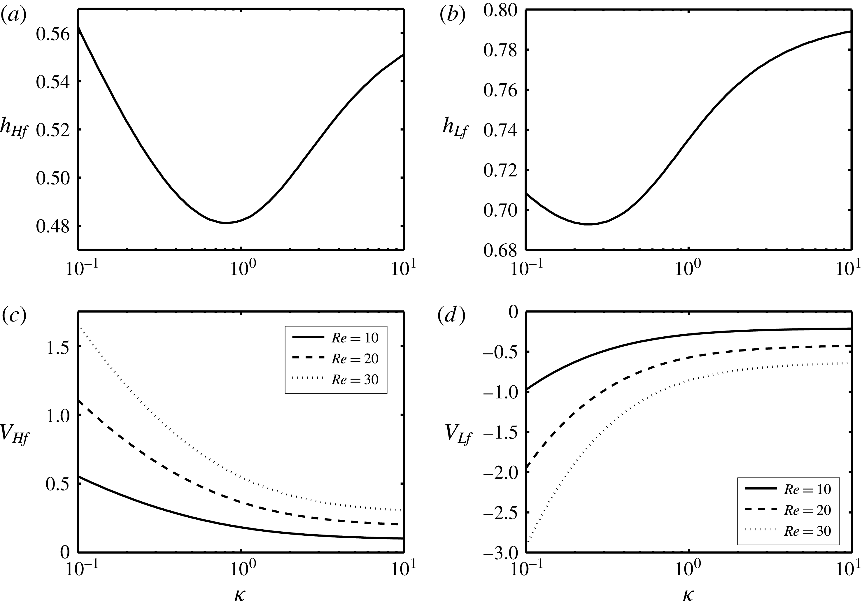
The variation of the height and speed of heavy and light fronts at long time with
 $\unicode[STIX]{x1D705}$
and
 $Re$
is shown in figure 5 using the equal-area rule. Figure 5(a,b) demonstrates the variation of
 $h_{Hf}$
and
 $h_{Lf}$
, respectively, over a wide range of
 $\unicode[STIX]{x1D705}$
. As predicted in figure 4(a), the heights of heavy and light fronts will not change with the Reynolds number. Therefore, the curves for all values of
 $Re$
overlay in figure 5(a,b). The
 $h_{Hf}$
value reaches a minimum at
 $\unicode[STIX]{x1D705}\approx 0.8$
, while the minimum
 $h_{LF}$
value appears at a smaller viscosity contrast (
 $\unicode[STIX]{x1D705}\approx 0.2$
). Although
 $h_{Hf}$
and
 $h_{Lf}$
change non-monotonically with viscosity ratio, the variation of
 $V_{Hf}$
and
 $V_{Lf}$
with
 $\unicode[STIX]{x1D705}$
is monotonic, as shown in figure 5(c,d). Also note that, unlike the frontal height, the frontal speeds clearly depend on
 $Re$
(speeds increasing with
 $Re$
). The absolute values of
 $V_{Hf}$
and
 $V_{Lf}$
decrease with an increase in
 $\unicode[STIX]{x1D705}$
, as also revealed in figure 4(b).
5.2 Particle-laden flows
$(\unicode[STIX]{x1D719}_{0}>0)$

We now examine particle-laden flows. Solving the governing system of PDEs (3.18) and (3.19) numerically when
 $\unicode[STIX]{x1D719}_{0}\neq 0$
, is more challenging, since an extremely small mesh size (
 $\text{d}x\approx 2\times 10^{-7}$
) is required to fully capture the underlying effects of the flow (Cook et al.
Reference Cook, Bertozzi and Hosoi2008). Figure 6(a) shows the evolution of the interface height profile,
 $h$
, at times
 $t=[0,0.01,0.02,\ldots ,0.1]$
for
 $\unicode[STIX]{x1D719}_{0}=0.3$
,
 $Re=0.1$
and
 $\unicode[STIX]{x1D705}=1$
. The other parameters are chosen close to those in the experiments of Zhou et al. (Reference Zhou, Dupuy, Bertozzi and Hosoi2005) (
 $r_{p}=0.06$
,
 $\unicode[STIX]{x1D709}=1.9$
and
 $\unicode[STIX]{x1D702}=1.25$
). The particle volume fraction value mostly chosen in our study (
 $\unicode[STIX]{x1D719}_{0}=0.3$
) is selected such that a comparison with the results of Zhou et al. (Reference Zhou, Dupuy, Bertozzi and Hosoi2005) and Cook et al. (Reference Cook, Bertozzi and Hosoi2008) can be made feasible. Understanding the suspension behaviour in the dense granular limit,
 $\unicode[STIX]{x1D719}_{0}\rightarrow \unicode[STIX]{x1D719}_{j}$
(Lyon & Leal Reference Lyon and Leal1998), requires further study, which is outside the scope of the current paper. Note that the viscosity function (3.4) becomes singular as
 $\unicode[STIX]{x1D719}_{0}\rightarrow \unicode[STIX]{x1D719}_{j}$
. In the case of particle-laden flows, a zero precursor film thickness introduces a singularity into the solution, as laid out by Cook et al. (Reference Cook, Bertozzi and Hosoi2008). To overcome such a singularity, we have used a small value of
 $b=0.01$
in this paper unless otherwise stated; see also the experiments of Zhou et al. (Reference Zhou, Dupuy, Bertozzi and Hosoi2005) and the computations of Cook et al. (Reference Cook, Bertozzi and Hosoi2008). The small choice of
 $t=0.1$
for the case of figure 6 is due to the limited access to computational resources for carrying out these simulations. Nevertheless, even this small interval is enough to extrapolate the long-time behaviour of the flow, thanks to the self-similarity characteristic of the solutions. The top insets in figure 6(a,b) show the collapse of profiles using
 $\unicode[STIX]{x1D706}=x/t$
with a small residual dependence on time that is comparable to that found by Taghavi et al. (Reference Taghavi, Seon, Martinez and Frigaard2009) and Hasnain & Alba (Reference Hasnain and Alba2017) for displacement flows. Owing to the complex interface shape, the Rankine–Hugoniot similarity conditions of Zhou et al. (Reference Zhou, Dupuy, Bertozzi and Hosoi2005) may not be directly applied to the particle-laden exchange flows in confined geometry. The computed solution mesh independence is successfully confirmed in figure 6(a) for two different values of
 $\text{d}x$
.
Evolution of the (a) interface height,
 $h$
, and (b) particle volume fraction,
 $\unicode[STIX]{x1D719}$
, profiles with time,
 $t=[0,0.01,0.02,\ldots ,0.1]$
. The parameters used are
 $\unicode[STIX]{x1D719}_{0}=0.3$
,
 $Re=0.1$
,
 $\unicode[STIX]{x1D705}=1$
,
 $r_{p}=0.06$
,
 $\unicode[STIX]{x1D709}=1.9$
and
 $\unicode[STIX]{x1D702}=1.25$
. The blue dashed lines show the solution at
 $t=0.1$
for
 $\text{d}x=2\times 10^{-6}$
, which is almost indistinguishable from that of
 $\text{d}x=2\times 10^{-7}$
. The lower left inset in (a) shows the corresponding interface profile in the pure fluid case obtained for the same
 $Re$
and
 $m$
values. The upper right inset in (a) and the one in (b) show the collapse of the profiles using the self-similarity parameter,
 $\unicode[STIX]{x1D706}=x/t$
.
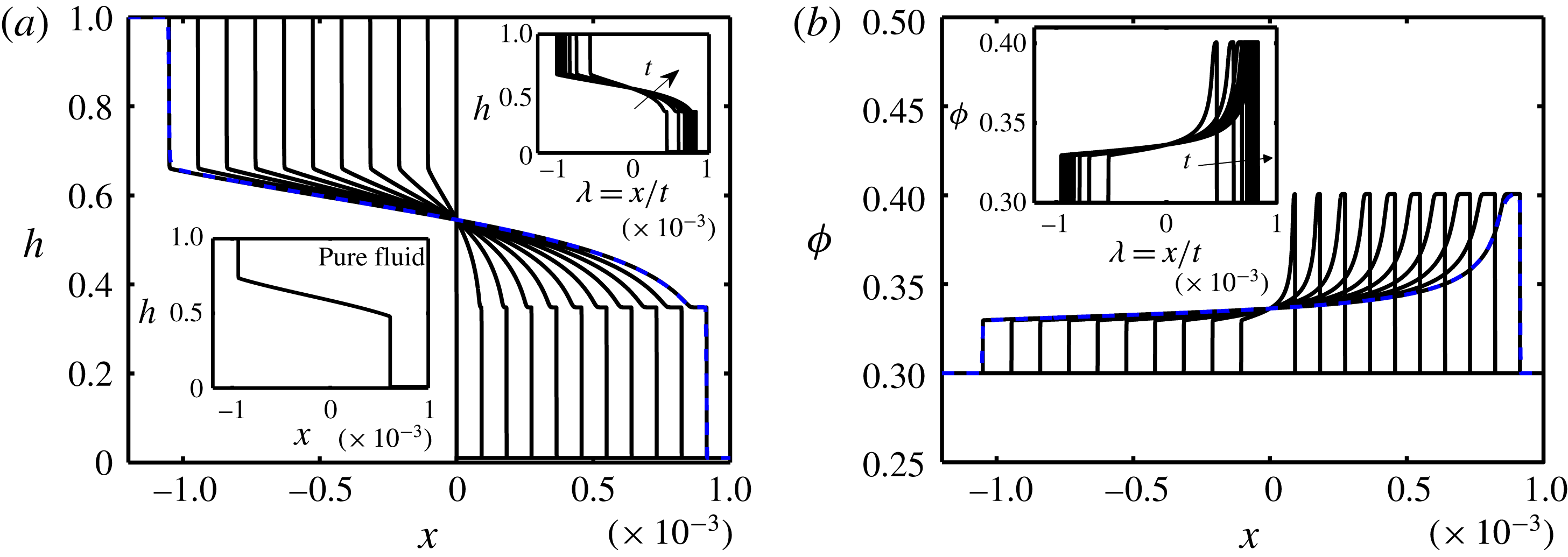
In order to fully understand the effect of particle addition to exchange flows, we have added interface height profiles corresponding to the pure fluids as insets to the particle-laden figure results; see figures 6–13. The Reynolds number,
 $Re$
, and mixture viscosity ratio,
 $m=m(\unicode[STIX]{x1D719}_{0},\unicode[STIX]{x1D705})$
, are kept the same in associated pure fluid and particle-laden cases. Upon comparing figure 6(a) to pure fluid results shown in the lower left inset, two important conclusions may be drawn. (1) The interface height profile in the presence of solid particles exhibits a plateau in the vicinity of the heavy layer front (
 $h\approx 0.348$
and
 $\unicode[STIX]{x1D719}\approx 0.400$
as steady long-time behaviour). Such a plateau is reminiscent of the capillary ridge in the simulations of Hasnain & Alba (Reference Hasnain and Alba2017) but is formed under a completely different mechanism, namely the presence of solid particles. (2) The stretched interface between the heavy and light fronts also is more curved in the particle-laden case compared to the pure fluid. In order to understand these differences, we need to look at the volume fraction profiles,
 $\unicode[STIX]{x1D719}$
, as shown in figure 6(b). As is interestingly evident, there are jumps in
 $\unicode[STIX]{x1D719}$
along the duct length,
 $x$
. In particular, there is an increase in
 $\unicode[STIX]{x1D719}$
close to the light layer front followed by a stronger jump in the vicinity of the heavy layer front. This pattern is different from that reported experimentally and theoretically by Zhou et al. (Reference Zhou, Dupuy, Bertozzi and Hosoi2005) for free-surface film flows. Owing to the lock exchange configuration and geometry confinement, we witness a two-step increase in
 $\unicode[STIX]{x1D719}$
close to the heavy and light layers instead of the one observed in the vicinity of the heavy front in the case of Zhou et al. (Reference Zhou, Dupuy, Bertozzi and Hosoi2005). The curvature of the interface height in the particle-laden case is then justified by the fact that the viscosity of the heavy solution is continuously changing along the streamwise direction through
 $\unicode[STIX]{x1D719}$
in (3.4), in turn modifying the dynamics of the exchange flow (see also figure 4
b).
It has been hypothesized by Zhou et al. (Reference Zhou, Dupuy, Bertozzi and Hosoi2005) that the accumulation of particles close to the frontal region of the flow (e.g. in figure 6
b) is due to the different transport rates of fluid and solid shown mathematically in (3.23) and (3.24). See also Auzerais, Jackson & Russel (Reference Auzerais, Jackson and Russel1988) for similar shock formation effects in sedimentation problems. One question that might arise here is whether particle accumulation at the front can grow to an extent that causes pinch-off. In fact, by looking closely into the experiments of Zhou et al. (Reference Zhou, Dupuy, Bertozzi and Hosoi2005), Grunewald et al. (Reference Grunewald, Levy, Mata, Ward and Bertozzi2010), Mata & Bertozzi (Reference Mata and Bertozzi2011), Murisic et al. (Reference Murisic, Ho, Hu, Latterman, Koch, Lin, Mata and Bertozzi2011, Reference Murisic, Pausader, Peschka and Bertozzi2013), Mavromoustaki & Bertozzi (Reference Mavromoustaki and Bertozzi2014), Wang et al. (Reference Wang, Mavromoustaki, Bertozzi, Urdaneta and Huang2015) and Wong & Bertozzi (Reference Wong and Bertozzi2016) for particle-laden film flow down an incline, there is no evidence that such accumulation may lead to pinch-off. Also note that our computational code fails when particle enrichment approaches the jamming limit (
 $\unicode[STIX]{x1D707}\rightarrow \infty$
as
 $\unicode[STIX]{x1D719}\rightarrow \unicode[STIX]{x1D719}_{j}$
). The lubrication model assumption will also not be valid close to this limit. As can be seen, in all presented simulations, the computed
 $\unicode[STIX]{x1D719}$
values are well below this jamming limit. Owing to settling Stokes velocity of particles (negative buoyancy), the particles accumulate close to the front. However, this accumulation does not grow unboundedly because at the same time the properties of the mixture, such as density (3.3) and viscosity (3.4), are also changing as a result of enrichment, eventually taking the frontal flow dynamics to a balanced state.
Change in (a) interface height,
 $h$
, and (b) particle volume fraction,
 $\unicode[STIX]{x1D719}$
, with
 $x$
at
 $t=0.1$
and various values of the precursor film thickness,
 $b$
. Other parameters used are
 $\unicode[STIX]{x1D719}_{0}=0.3$
,
 $Re=0.1$
,
 $\unicode[STIX]{x1D705}=1$
,
 $r_{p}=0.06$
,
 $\unicode[STIX]{x1D709}=1.9$
and
 $\unicode[STIX]{x1D702}=1.25$
. The inset in (a) shows the corresponding interface profiles to the pure fluid case obtained for the same
 $Re$
and
 $m$
values.
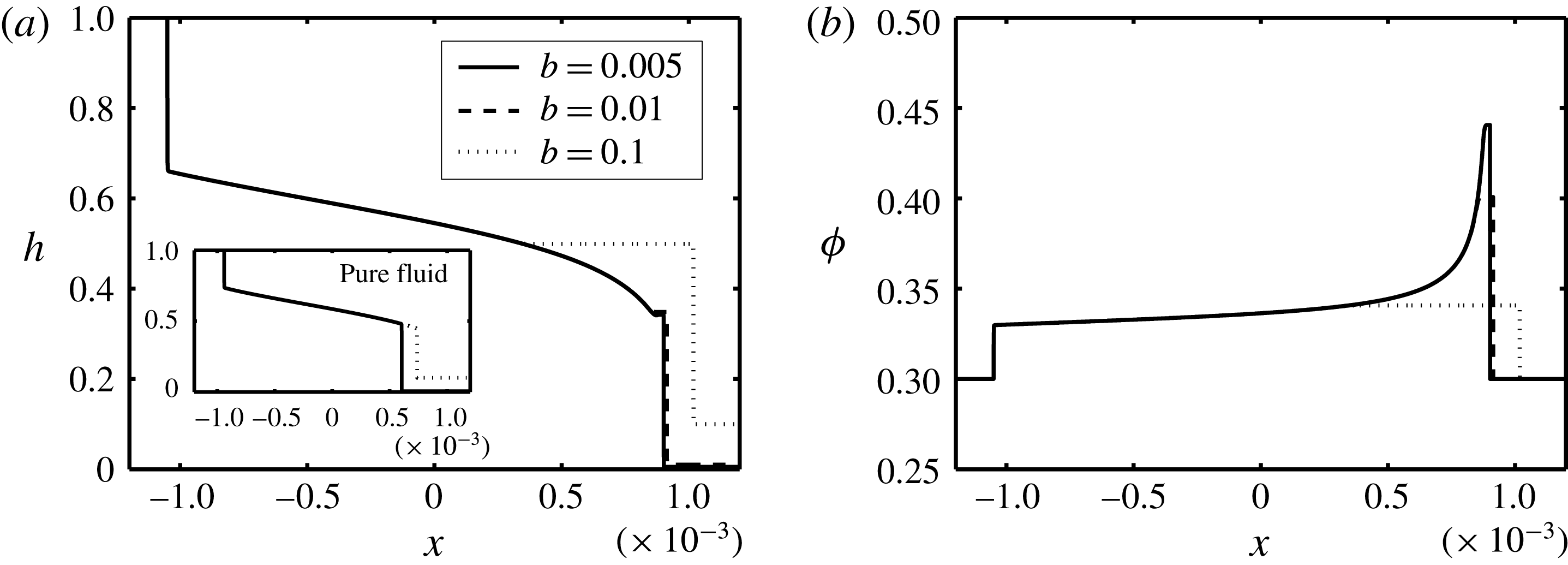
The effect of the precursor film thickness,
 $b$
, is investigated in figure 7, keeping the rest of the controlling parameters the same as in figure 6. Figure 7(a) shows that, even though the shape of the light layer front remains unchanged, the one for the heavy layer is significantly affected by
 $b$
; also compare against the inset representing the pure fluid case. The height of the heavy layer front and its extent increase with
 $b$
. An increase in the frontal height is accompanied by a decrease in the level of particle enrichment, as evident in figure 7(b). For small values of
 $b$
, the particle-rich zone grows to an extent that might cause singularity in the solution (
 $\unicode[STIX]{x1D707}_{H}\rightarrow \infty$
as
 $\unicode[STIX]{x1D719}\rightarrow \unicode[STIX]{x1D719}_{j}$
). This observation is in complete agreement with the findings of Zhou et al. (Reference Zhou, Dupuy, Bertozzi and Hosoi2005) and Cook et al. (Reference Cook, Bertozzi and Hosoi2008) for free-surface film flows. In fact, they mention that this complex frontal shock behaviour may not be entirely captured by a first-order lubrication model. A singular shock behaviour in our model may also be observed at high initial volume fractions. As discussed by Cook et al. (Reference Cook, Bertozzi and Hosoi2008), using the Buscall settling function instead of Richardson–Zaki may alleviate such a singularity, which requires further study. Figures 8(a) and 8(b) compare the profiles of the interface height,
 $h$
, and particle volume fraction,
 $\unicode[STIX]{x1D719}$
, respectively, at various values of the Reynolds number,
 $Re$
. In compliance with our observation in figure 8(a) inset for pure fluids, the interpenetration rate of the heavy and light layers similarly increases with
 $Re$
. Moreover, the heights of the heavy and light fronts remain the same while changing
 $Re$
. The constancy in advancing front heights is accompanied by uniform increase in volume fraction of particles; see figure 8(b).
Change in (a) interface height,
 $h$
, and (b) particle volume fraction,
 $\unicode[STIX]{x1D719}$
, with
 $x$
at
 $t=0.1$
and various values of the Reynolds number,
 $Re$
. Other parameters used are
 $\unicode[STIX]{x1D719}_{0}=0.3$
,
 $\unicode[STIX]{x1D705}=1$
,
 $r_{p}=0.06$
,
 $\unicode[STIX]{x1D709}=1.9$
and
 $\unicode[STIX]{x1D702}=1.25$
. The inset in (a) shows the corresponding interface profiles to the pure fluid case obtained for the same
 $Re$
and
 $m$
values.

Change in (a) interface height,
 $h$
, and (b) particle volume fraction,
 $\unicode[STIX]{x1D719}$
, with
 $x$
at
 $t=0.1$
and various values of the initial particle volume fraction,
 $\unicode[STIX]{x1D719}_{0}$
. Other parameters used are
 $Re=0.1$
,
 $\unicode[STIX]{x1D705}=1$
,
 $r_{p}=0.06$
,
 $\unicode[STIX]{x1D709}=1.9$
and
 $\unicode[STIX]{x1D702}=1.25$
. The inset in (a) shows the corresponding interface profiles to the pure fluid case obtained for the same
 $Re$
and
 $m$
values.
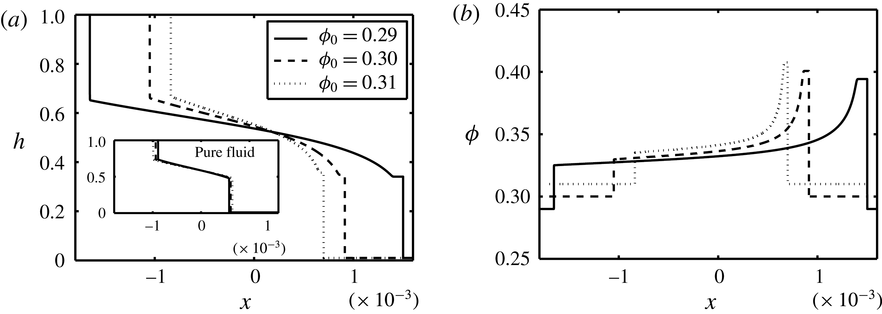
The initial volume fraction of particles,
 $\unicode[STIX]{x1D719}_{0}$
, plays an important role in the dynamics of the flow, as it controls both the density (3.3) and viscosity (3.4) of the heavy mixture. Keeping all the other parameters constant, the dependence of the interface height,
 $h$
, and volume fraction of particles,
 $\unicode[STIX]{x1D719}$
, on
 $\unicode[STIX]{x1D719}_{0}$
is investigated in figures 9(a) and 9(b) respectively. The extent of the exchange flow is decreased with
 $\unicode[STIX]{x1D719}_{0}$
as shown in figure 9(a). While the density of the heavy mixture,
 $\hat{\unicode[STIX]{x1D70C}}_{H}$
, increases with
 $\unicode[STIX]{x1D719}_{0}$
(larger driving force), its viscosity,
 $\hat{\unicode[STIX]{x1D707}}_{H}$
, also increases, which results in an overall slowdown of the flow. The frontal heights of the heavy and light layers are shown to minutely increase with
 $\unicode[STIX]{x1D719}_{0}$
. The corresponding profiles to the pure fluid case are shown in the inset of figure 9(a). An increase in
 $\unicode[STIX]{x1D719}_{0}$
results in a decrease in the effective mixture viscosity ratio,
 $m$
, which can mildly extend the exchange zone between the two fluids observed from the inset of figure 9(a); see also figure 4(b). Particle enrichment close to the heavy and light fronts is consistently observed over a range of
 $\unicode[STIX]{x1D719}_{0}$
(figure 9
b). However, the relative rise in particle concentration seems to be slightly less for higher
 $\unicode[STIX]{x1D719}_{0}$
; compare, for example, the
 $\unicode[STIX]{x1D719}_{0}=0.29$
and
 $0.31$
curves in figure 9(b). The general features of the flow, such as interface height curvature as well as particle enrichment close to the heavy front, for other values of
 $\unicode[STIX]{x1D719}_{0}$
, e.g. in the dilute range
 $\unicode[STIX]{x1D719}_{0}=0.01$
(Segre & Silberberg Reference Segre and Silberberg1961), are similar to those obtained for
 $\unicode[STIX]{x1D719}_{0}\approx 0.3$
. Results are not presented here for brevity.
Change in (a) interface height,
 $h$
, and (b) particle volume fraction,
 $\unicode[STIX]{x1D719}$
, with
 $x$
at
 $t=0.1$
and various values of the light-to-carrying-fluid viscosity ratio,
 $\unicode[STIX]{x1D705}$
. Other parameters used are
 $\unicode[STIX]{x1D719}_{0}=0.3$
,
 $Re=0.1$
,
 $r_{p}=0.06$
,
 $\unicode[STIX]{x1D709}=1.9$
and
 $\unicode[STIX]{x1D702}=1.25$
. The inset in (a) shows the corresponding interface profiles to the pure fluid case obtained for the same
 $Re$
and
 $m$
values.
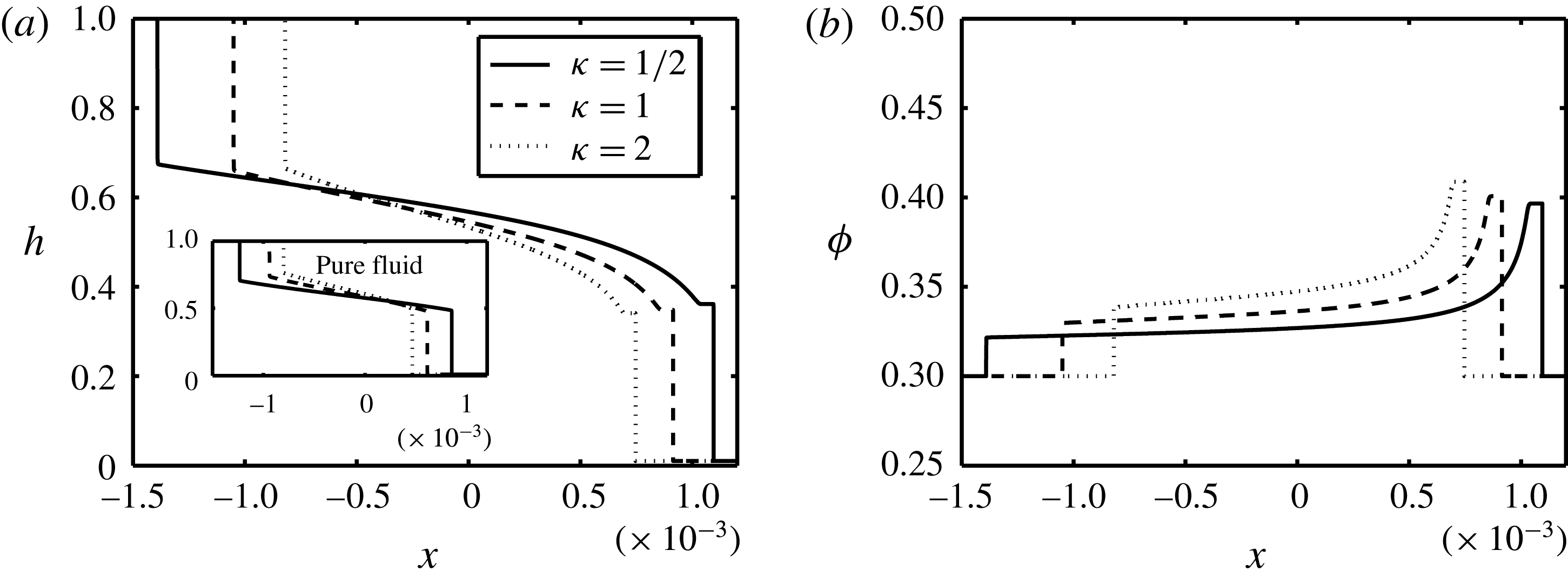
The increase in light-to-carrying-fluid viscosity ratio,
 $\unicode[STIX]{x1D705}$
, tends to contract the exchange zone between the two fluids, as shown in figure 10(a). Comparing this to the results for pure exchange flows shown as the inset, we infer that the height of the heavy front in the particle-laden case slightly decreases with
 $\unicode[STIX]{x1D705}$
, which is complemented by a growth in the volume fraction of particles,
 $\unicode[STIX]{x1D719}$
(figure 10
b). Note that in the case of free-surface film flow of Zhou et al. (Reference Zhou, Dupuy, Bertozzi and Hosoi2005) and Cook et al. (Reference Cook, Bertozzi and Hosoi2008), an increase (decrease) in the frontal height is only achieved by an increase (decrease) in local particle volume fraction. However, in a confined geometry, various intricate scenarios might happen at the front; for example, the frontal height might decrease while particle volume fraction increases (figure 10) and vice versa (figure 7). Let us physically explain the increase of
 $\unicode[STIX]{x1D719}$
with
 $\unicode[STIX]{x1D705}$
observed in figure 10(b). Large
 $\unicode[STIX]{x1D705}$
corresponds to small
 $\hat{\unicode[STIX]{x1D707}}_{f,H}$
. Considering the definition, the dimensionless Stokes velocity,
 $u_{0}=2\hat{a}^{2}(\hat{\unicode[STIX]{x1D70C}}_{p}-\hat{\unicode[STIX]{x1D70C}}_{f,H}){\hat{g}}/(9\hat{V}_{t}\hat{\unicode[STIX]{x1D707}}_{f,H})$
, is increased as
 $\hat{\unicode[STIX]{x1D707}}_{f,H}$
is decreased. Larger
 $u_{0}$
increases particle slip velocity in the
 $G$
flux function (3.24), which will consequently result in stronger accumulation of particles, as shown in figure 10(b). In the case of Zhou et al. (Reference Zhou, Dupuy, Bertozzi and Hosoi2005) and Cook et al. (Reference Cook, Bertozzi and Hosoi2008), the flow dynamics is basically governed by particles settling within a single carrying fluid plus the no-stress condition imposed at the free surface. However, in the current channel flow case, we have not only the effect of the particles’ slip velocity but also the interaction of the carrying and light fluids at the interface captured via the stress homogeneity condition (3.13). Such a combination gives rise to complex patterns observed in the channel geometry as opposed to the free-surface geometry.
Change in (a) interface height,
 $h$
, and (b) particle volume fraction,
 $\unicode[STIX]{x1D719}$
, with
 $x$
at
 $t=0.1$
and various values of the particle-radius-to-half-duct-width ratio,
 $r_{p}$
. Other parameters used are
 $\unicode[STIX]{x1D719}_{0}=0.3$
,
 $Re=0.1$
,
 $\unicode[STIX]{x1D705}=1$
,
 $\unicode[STIX]{x1D709}=1.9$
and
 $\unicode[STIX]{x1D702}=1.25$
. The inset in (a) shows the corresponding interface profile to the pure fluid case obtained for the same
 $Re$
and
 $m$
values.
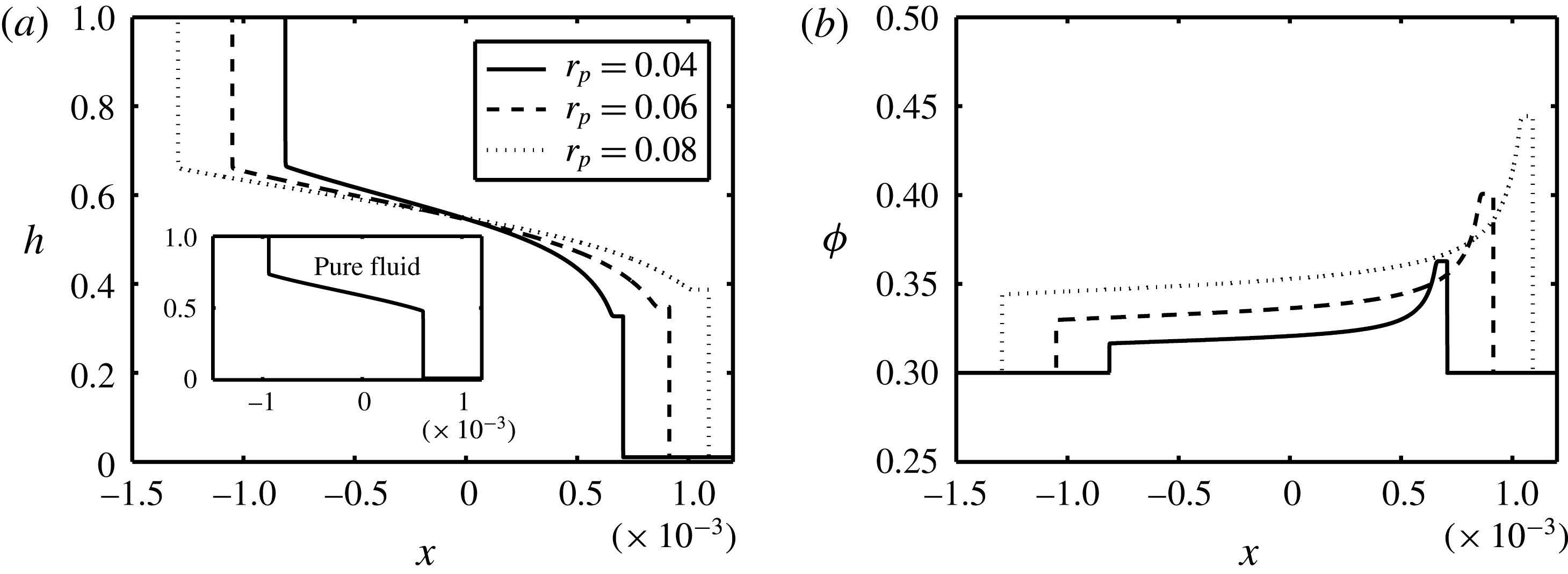
Investigating the effect of the relative size of particles,
 $r_{p}$
, can provide more insight into the dynamics of the exchange flow in question. Figure 11 shows the interface height and particle volume fraction profiles for the same parameters as in figure 6 except
 $r_{p}$
. An increase in the size of particles consistently increases the height of the heavy front (figure 11
a) and local volume fraction (figure 11
b). Note a similar increase in
 $\unicode[STIX]{x1D719}$
close to the light fluid front as well as the heavy one. As is evident in figure 11(a), the interface between the two fluids has been extended with
 $r_{p}$
. Let us have a fundamental look into this effect. The increase in
 $r_{p}=\hat{a}/\hat{D}$
can be interpreted as either an increase in particle radius,
 $\hat{a}$
, or a decrease in half the duct width,
 $\hat{D}$
. If we supposedly consider the latter, then from the Reynolds-number expression given in table 2,
 $Re$
should therefore decrease. Increasing
 $r_{p}$
while keeping
 $Re$
the same in figure 11 requires, for instance, a decrease in the heavy mixture viscosity,
 $\hat{\unicode[STIX]{x1D707}}_{H}(\unicode[STIX]{x1D719}_{0})$
, which is achievable by decreasing the carrying fluid viscosity,
 $\hat{\unicode[STIX]{x1D707}}_{f,H}$
; see § 2. In order to keep
 $\unicode[STIX]{x1D705}=\hat{\unicode[STIX]{x1D707}}_{L}/\hat{\unicode[STIX]{x1D707}}_{f,H}$
the same in figure 11,
 $\hat{\unicode[STIX]{x1D707}}_{L}$
will also be decreased. A decrease in the carrying and light fluids viscosity, on the other hand, acts to ease the advancement of the exchange flow as confirmed in figure 11(a). The effect of
 $r_{p}$
is also directly reflected in the particles’ dimensionless Stokes velocity,
 $u_{0}=(\unicode[STIX]{x1D709}-1)\unicode[STIX]{x1D713}\unicode[STIX]{x1D705}Re(1+\unicode[STIX]{x1D713})r_{p}^{2}/(9m\unicode[STIX]{x1D702}(1-\unicode[STIX]{x1D713}))$
, which feeds into the flux function
 $G$
in (3.24). An increase in
 $r_{p}$
enhances the settling speed of the particles, which in turn causes accumulation of particles close to the advancing frontal regions.
Another factor that can potentially enhance the Stokes settling velocity of the particles is the particle-to-carrying-fluid density ratio,
 $\unicode[STIX]{x1D709}$
; see figure 12. As opposed to
 $r_{p}$
, an increase in
 $\unicode[STIX]{x1D709}$
reduces the interpenetration rate of the heavy and light layers; see figure 12(a). At first glance, this effect seems rather counterintuitive since an increase in
 $\unicode[STIX]{x1D709}$
indicates heavier particles, which should, in turn, increase the buoyant driving force of the flow. However, similar to the rationale presented for figure 11, we need to consider the fact that the depicted profiles are obtained for constant Reynolds number,
 $Re=\hat{\unicode[STIX]{x1D70C}}_{H}(\unicode[STIX]{x1D719}_{0})\hat{V}_{t}(2\hat{D})/\hat{\unicode[STIX]{x1D707}}_{H}(\unicode[STIX]{x1D719}_{0})$
. From § 2, we learnt that
 $Re$
depends on
 $\hat{V}_{t}$
, which, by itself, decreases with
 $\unicode[STIX]{x1D713}$
since
 $\hat{V}_{t}=\sqrt{(1-\unicode[STIX]{x1D713}){\hat{g}}\hat{D}/(1+\unicode[STIX]{x1D713})}$
. The parameter
 $\unicode[STIX]{x1D713}=\unicode[STIX]{x1D702}/(1+(\unicode[STIX]{x1D709}-1)\unicode[STIX]{x1D719}_{0})$
is inversely related to
 $\unicode[STIX]{x1D709}$
. Therefore, increasing
 $\unicode[STIX]{x1D709}$
(thus
 $\hat{V}_{t}$
) meanwhile keeping
 $Re$
constant may be deduced as an increase in
 $\hat{\unicode[STIX]{x1D707}}_{H}(\unicode[STIX]{x1D719}_{0})=\hat{\unicode[STIX]{x1D707}}_{f,H}(1-\unicode[STIX]{x1D719}_{0}/\unicode[STIX]{x1D719}_{j})^{-2}$
or
 $\hat{\unicode[STIX]{x1D707}}_{f,H}$
. Since
 $\unicode[STIX]{x1D705}=\hat{\unicode[STIX]{x1D707}}_{L}/\hat{\unicode[STIX]{x1D707}}_{f,H}=1$
, we shall also have
 $\hat{\unicode[STIX]{x1D707}}_{L}$
increasing. As a result, flow deceleration will occur for high
 $\unicode[STIX]{x1D709}$
, which is correspondingly confirmed in figure 12(a). Furthermore, the increase in volume fraction of particles for high
 $\unicode[STIX]{x1D709}$
(settling in high-viscosity medium) is slightly less than, but still comparable to, that of low
 $\unicode[STIX]{x1D709}$
due to the higher density of solids in the former (figure 12
b).
Change in (a) interface height,
 $h$
, and (b) particle volume fraction,
 $\unicode[STIX]{x1D719}$
, with
 $x$
at
 $t=0.1$
and various values of the particle-to-carrying-fluid density ratio,
 $\unicode[STIX]{x1D709}$
. Other parameters used are
 $\unicode[STIX]{x1D719}_{0}=0.3$
,
 $Re=0.1$
,
 $\unicode[STIX]{x1D705}=1$
,
 $r_{p}=0.06$
and
 $\unicode[STIX]{x1D702}=1.25$
. The inset in (a) shows the corresponding interface profile to the pure fluid case obtained for the same
 $Re$
and
 $m$
values.

Change in (a) interface height,
 $h$
, and (b) particle volume fraction,
 $\unicode[STIX]{x1D719}$
, with
 $x$
at
 $t=0.1$
and various values of the light-to-carrying-fluid density ratio,
 $\unicode[STIX]{x1D702}$
. Other parameters used are
 $\unicode[STIX]{x1D719}_{0}=0.3$
,
 $Re=0.1$
,
 $\unicode[STIX]{x1D705}=1$
,
 $r_{p}=0.06$
and
 $\unicode[STIX]{x1D709}=1.9$
. The inset in (a) shows the corresponding interface profile to the pure fluid case obtained for the same
 $Re$
and
 $m$
values.

Finally, the variations of the interface height,
 $h$
, and particle volume fraction,
 $\unicode[STIX]{x1D719}$
, versus the light-to-carrying-fluid density ratio,
 $\unicode[STIX]{x1D702}$
, are examined in figures 13(a) and 13(b), respectively. Even though the presented
 $\unicode[STIX]{x1D702}$
values are all larger than unity, i.e. light fluid denser than carrying fluid, the overall density of the suspension mixture is always larger than the light pure fluid (
 $\unicode[STIX]{x1D713}<1$
). Note that the interpenetration extent of the mixtures has increased with
 $\unicode[STIX]{x1D702}$
(figure 13
a). Similar to figure 12, this effect also appears counterintuitive at first. This is because an increase in
 $\unicode[STIX]{x1D702}$
means a denser light fluid in the lower section of the duct compared to the carrying fluid at the top, i.e. a decrease in the effective density difference between the heavy and light mixtures. Increasing
 $\unicode[STIX]{x1D702}$
meanwhile keeping
 $Re$
the same in figure 13(a) requires, for instance, a reduction in the viscosity of the involved fluids (
 $Re\propto \hat{\unicode[STIX]{x1D70C}}_{H}(\unicode[STIX]{x1D719}_{0})/\hat{\unicode[STIX]{x1D707}}_{H}(\unicode[STIX]{x1D719}_{0})$
), which consequently enhances flow acceleration. The front height on the heavy side slightly decreases with an increase in
 $\unicode[STIX]{x1D702}$
. As
 $\unicode[STIX]{x1D702}$
increases (while keeping
 $Re$
constant), the mixture’s viscosity decreases, facilitating particle settling and thus enrichment in volume fraction,
 $\unicode[STIX]{x1D719}$
, close to the fronts (figure 13
b). Since
 $r_{p}$
,
 $\unicode[STIX]{x1D709}$
and
 $\unicode[STIX]{x1D702}$
do not affect the mixture’s viscosity ratio,
 $m=\unicode[STIX]{x1D705}(1-\unicode[STIX]{x1D719}_{0}/\unicode[STIX]{x1D719}_{j})^{2}$
, the shape of the interface height obtained in the pure fluid limit remains unchanged with these parameters; see insets shown in figures 11(a)–13(a).
6 Conclusions
Buoyancy-driven exchange flow of two mixtures in a vertical duct (2D channel as well as pipe) is investigated theoretically. The light mixture is always assumed to be a pure fluid, whereas the heavy mixture can be either pure or particle-laden. Assuming a small aspect ratio for the duct,
 $\unicode[STIX]{x1D6FF}$
, a lubrication model is developed. The methodology of Zhou et al. (Reference Zhou, Dupuy, Bertozzi and Hosoi2005) for free-surface particle-laden film flows is employed and extended to a lock exchange system in a confined geometry under the Boussinesq limit. The derived model takes the simple form of the classical Riemann problem. A robust TVD finite difference scheme is implemented to solve the model PDEs numerically. The solutions suggest self-similar interface shapes over time. In the limit of small aspect ratio (
 $\unicode[STIX]{x1D6FF}\ll 1$
) and assuming a jamming volume fraction of
 $\unicode[STIX]{x1D719}_{j}\approx 0.67$
, six dimensionless parameters govern the flow, namely, particle-radius-to-half-duct-width ratio,
 $r_{p}$
, particle-to-carrying-fluid density ratio,
 $\unicode[STIX]{x1D709}$
, light-to-carrying-fluid density ratio,
 $\unicode[STIX]{x1D702}$
, light-to-carrying-fluid viscosity ratio,
 $\unicode[STIX]{x1D705}$
, initial volume fraction of particles,
 $\unicode[STIX]{x1D719}_{0}$
, and the Reynolds number,
 $Re$
. Owing to the choice of scaling, the dynamics of the flow for pure fluids (
 $\unicode[STIX]{x1D719}_{0}=r_{p}=\unicode[STIX]{x1D709}=0$
) is governed only by
 $\unicode[STIX]{x1D705}$
and
 $Re$
. The physical effect of these parameters on the dynamics of the flow has been quantified through a systematic approach. It is observed that the interpenetration rate of the heavy and light layers increases with
 $Re$
and decreases with
 $\unicode[STIX]{x1D705}$
. The heights of the heavy and light fronts change with
 $\unicode[STIX]{x1D705}$
but remain unchanged with
 $Re$
. The dynamics of the exchange flow becomes entirely different in the presence of solid particles compared to pure fluids. Primarily, the interface profiles are more curved in the former with respect to the latter due to change of viscosity along the duct. Novel particle-rich zones inside the suspension are further discovered in the vicinity of the advancing heavy and light fronts. The particle enrichment at the fronts is associated with different transport rates of fluid and solid due to the Stokes settling velocity of the particles. It is also revealed that geometry confinement plays a significant role in exchange flow dynamics such as formation of interfacial patterns and particle-enrichment behaviour. Whereas, in the unconfined geometry, particle enrichment was shown to be accompanied by an increase in the interface height profile, in a confined duct, either an increase or a decrease in height is possible depending on the controlling parameters of the flow. The level of particle enrichment remains the same with
 $Re$
, is enhanced by
 $\unicode[STIX]{x1D705}$
,
 $r_{p}$
and
 $\unicode[STIX]{x1D702}$
, and is slightly reduced with
 $\unicode[STIX]{x1D719}_{0}$
and
 $\unicode[STIX]{x1D709}$
. The stretched interface between the heavy and light fronts grows with
 $r_{p}$
,
 $\unicode[STIX]{x1D702}$
and
 $Re$
, but shrinks with
 $\unicode[STIX]{x1D719}_{0}$
,
 $\unicode[STIX]{x1D705}$
and
 $\unicode[STIX]{x1D709}$
. The model can be easily extended to include interfacial tension effects; see Hasnain & Alba (Reference Hasnain and Alba2017) for similar implementation in the case of pure fluids.
Acknowledgements
This research has been carried out at the University of Houston through National Research University Fund (NRUF). We thank the Center for Advanced Computing & Data Systems (CACDS) at the University of Houston and its helpful staff for providing us with their outstanding computational resources and assistance.
Appendix A. Shear-induced migration effects
Migration of particles induced by shear is in fact an important effect widely observed in particle-laden flows. Our methodology follows the approach of Zhou et al. (Reference Zhou, Dupuy, Bertozzi and Hosoi2005) for gravity-driven suspension film flow down an incline, which neglects the shear-induced migration effect (Schaflinger, Acrivos & Zhang Reference Schaflinger, Acrivos and Zhang1990; Acrivos, Fan & Mauri Reference Acrivos, Fan and Mauri1994). In this appendix we would like to verify the conditions under which such an assumption is valid. The particle transport equation for particle-laden film flows is given by Murisic et al. (Reference Murisic, Pausader, Peschka and Bertozzi2013) and Wong & Bertozzi (Reference Wong and Bertozzi2016) as
 $$\begin{eqnarray}\displaystyle & \displaystyle \unicode[STIX]{x1D719}_{\hat{t}}+\hat{u} \unicode[STIX]{x1D719}_{\hat{x}}+\hat{v}\unicode[STIX]{x1D719}_{{\hat{y}}}=-\hat{\boldsymbol{J}}_{\hat{x},\hat{x}}-\hat{\boldsymbol{J}}_{{\hat{y}},{\hat{y}}}. & \displaystyle\end{eqnarray}$$
Here,
 $\hat{\boldsymbol{J}}$
is the particle flux due to settling and migration,
 $$\begin{eqnarray}\displaystyle & \displaystyle \hat{\boldsymbol{J}}=\hat{\boldsymbol{J}}_{settling}+\hat{\boldsymbol{J}}_{migration}. & \displaystyle\end{eqnarray}$$
The settling and migration flux components can be expressed as the following (Murisic et al. Reference Murisic, Pausader, Peschka and Bertozzi2013; Wong & Bertozzi Reference Wong and Bertozzi2016):
 $$\begin{eqnarray}\displaystyle & \displaystyle \hat{\boldsymbol{J}}_{settling}={\displaystyle \frac{2\hat{a}^{2}{\hat{g}}(\hat{\unicode[STIX]{x1D70C}}_{p}-\hat{\unicode[STIX]{x1D70C}}_{f,H})}{9\hat{\unicode[STIX]{x1D707}}_{f,H}}}(1-\unicode[STIX]{x1D719})\unicode[STIX]{x1D719}, & \displaystyle\end{eqnarray}$$
 $$\begin{eqnarray}\displaystyle & \displaystyle \hat{\boldsymbol{J}}_{migration}=-{\displaystyle \frac{\hat{a}^{2}\hat{V}_{t}}{\hat{D}^{2}}}\left[K_{c}\unicode[STIX]{x1D719}\unicode[STIX]{x1D735}(\unicode[STIX]{x1D719}u_{y})+{\displaystyle \frac{K_{v}\unicode[STIX]{x1D719}^{2}u_{y}}{\unicode[STIX]{x1D707}_{H}}}\unicode[STIX]{x1D735}\unicode[STIX]{x1D707}_{H}\right]. & \displaystyle\end{eqnarray}$$
The constants
 $K_{c}\approx 0.41$
and
 $K_{v}\approx 0.62$
correspond to shear-induced particle flux due to gradients in the particle volume fraction and effective viscosity of the suspension, which are determined empirically (Phillips et al.
Reference Phillips, Armstrong, Brown, Graham and Abbott1992; Wong & Bertozzi Reference Wong and Bertozzi2016). From the velocity expression (3.15), it can be found that
 $u_{y}\sim Re$
; see also appendix C for the coefficients. Therefore, the largest flux component due to shear-induced migration in (A 4) is of order
 $K_{v}\hat{a}^{2}\hat{V}_{t}Re/\hat{D}^{2}$
, whereas that of settling is the coefficient of the
 $(1-\unicode[STIX]{x1D719})\unicode[STIX]{x1D719}$
term in (A 3), i.e.
 $2\hat{a}^{2}{\hat{g}}(\hat{\unicode[STIX]{x1D70C}}_{p}-\hat{\unicode[STIX]{x1D70C}}_{f,H})/(9\hat{\unicode[STIX]{x1D707}}_{f,H})$
. Note that the rest of the terms in (A 3) and (A 4) being multiplied by these coefficients are
 $O(1)$
since they are made dimensionless. By requiring that the settling effects overcome those of migration (
 $\hat{\boldsymbol{J}}_{settling}\gg \hat{\boldsymbol{J}}_{migration}$
), the following condition is finally obtained:
 $$\begin{eqnarray}\displaystyle & \displaystyle {\displaystyle \frac{9K_{v}\unicode[STIX]{x1D702}(1-\unicode[STIX]{x1D719}_{0}/\unicode[STIX]{x1D719}_{j})^{2}}{\unicode[STIX]{x1D713}(\unicode[STIX]{x1D709}-1)}}{\displaystyle \frac{(1-\unicode[STIX]{x1D713})}{(1+\unicode[STIX]{x1D713})}}\ll 1. & \displaystyle\end{eqnarray}$$
Note that the
 $(1-\unicode[STIX]{x1D713})/(1+\unicode[STIX]{x1D713})$
term in (A 5) is nothing other than the effective Atwood number,
 $At=(\hat{\unicode[STIX]{x1D70C}}_{H}(\unicode[STIX]{x1D719}_{0})-\hat{\unicode[STIX]{x1D70C}}_{L})/(\hat{\unicode[STIX]{x1D70C}}_{H}(\unicode[STIX]{x1D719}_{0})+\hat{\unicode[STIX]{x1D70C}}_{L})$
. In other words, the Boussinesq limit (
 $At\ll 1$
), discussed by Taghavi et al. (Reference Taghavi, Alba, Seon, Wielage-Burchard, Martinez and Frigaard2012b
), ensures that the shear-induced migration effects are negligible in front of settling. Note that the rest of the terms in (A 5) are approximately
 $O(1)$
. From a fundamental standpoint, the small Atwood number or density difference between the mixtures does not cause a strong countercurrent and shear in the flow, which would lead to migration. However, in the meantime, the particles would have the opportunity to settle due to their weight. The condition (A 5) is indeed valid in the simulations presented in this paper. For instance, for a typical set of parameters chosen in our study, e.g. in figure 6, the left-hand side term in the condition above is approximately 0.019, i.e. settling flux more than 50 times stronger than that of shear-induced migration.
Schematic of axisymmetric particle-laden exchange flow in a vertical pipe.

Appendix B. Axisymmetric flow in pipe
Performing exchange flow experiments in a pipe geometry can be more feasible compared to the 2D channel geometry. Therefore, in this appendix the exchange flow model is extended to a practical pipe geometry; see figure 14. It is not difficult to show that in cylindrical coordinates the momentum equations (3.9) and (3.10) take the following forms:
 $$\begin{eqnarray}\displaystyle 0=-P_{0,x}+\unicode[STIX]{x1D707}_{H}(\unicode[STIX]{x1D719})(ru_{r})_{r}/r,\quad 1-h\leqslant r\leqslant 1, & & \displaystyle\end{eqnarray}$$
 $$\begin{eqnarray}\displaystyle 0=-P_{0,x}-(\unicode[STIX]{x1D70C}_{H}(\unicode[STIX]{x1D719})-\unicode[STIX]{x1D713})Re/(1-\unicode[STIX]{x1D713})+m(ru_{r})_{r}/r,\quad 0\leqslant r\leqslant 1-h. & & \displaystyle\end{eqnarray}$$
Applying appropriate boundary and interfacial conditions, equations (B 1) and (B 2) can be integrated with respect to
 $r$
in order to determine the streamwise velocity closures in each layer. The flux function,
 $q=\hat{q}/(\unicode[STIX]{x03C0}\hat{D}^{2}\hat{V}_{t})$
, as the flow rate within the heavy layer, can eventually be calculated as
 $$\begin{eqnarray}\displaystyle q=2\int _{1-h}^{1}ru\,\text{d}r, & & \displaystyle\end{eqnarray}$$
which is given below as a function of
 $h$
,
 $Re$
,
 $m$
,
 $\unicode[STIX]{x1D707}_{H}$
,
 $\unicode[STIX]{x1D70C}_{H}$
and
 $\unicode[STIX]{x1D713}$
:
 $$\begin{eqnarray}\displaystyle q & = & \displaystyle -(1/8)Re[\!-4\ln (1-h)\unicode[STIX]{x1D707}_{H}\unicode[STIX]{x1D713}-104h^{6}m\unicode[STIX]{x1D713}-144h^{5}\unicode[STIX]{x1D707}_{H}\unicode[STIX]{x1D713}+176h^{5}m\unicode[STIX]{x1D713}\nonumber\\ \displaystyle & & \displaystyle -\,80h^{3}m\unicode[STIX]{x1D70C}_{H}+16h^{2}m\unicode[STIX]{x1D70C}_{H}+164h^{4}m\unicode[STIX]{x1D70C}_{H}+144h^{5}\unicode[STIX]{x1D707}_{H}\unicode[STIX]{x1D70C}_{H}+104h^{6}m\unicode[STIX]{x1D70C}_{H}\nonumber\\ \displaystyle & & \displaystyle +\,80h^{6}\unicode[STIX]{x1D707}_{H}\unicode[STIX]{x1D713}+92h^{3}\unicode[STIX]{x1D707}_{H}\unicode[STIX]{x1D70C}_{H}-30h^{2}\unicode[STIX]{x1D707}_{H}\unicode[STIX]{x1D70C}_{H}+4h\unicode[STIX]{x1D707}_{H}\unicode[STIX]{x1D70C}_{H}-4h^{8}m\unicode[STIX]{x1D713}+32h^{7}m\unicode[STIX]{x1D713}\nonumber\\ \displaystyle & & \displaystyle +\,4h^{8}m\unicode[STIX]{x1D70C}_{H}-32h^{7}m\unicode[STIX]{x1D70C}_{H}-24h^{7}\unicode[STIX]{x1D707}_{H}\unicode[STIX]{x1D713}+24h^{7}\unicode[STIX]{x1D707}_{H}\unicode[STIX]{x1D70C}_{H}+3h^{8}\unicode[STIX]{x1D707}_{H}\unicode[STIX]{x1D713}-3h^{8}\unicode[STIX]{x1D707}_{H}\unicode[STIX]{x1D70C}_{H}\nonumber\\ \displaystyle & & \displaystyle +\,280\ln (1-h)h^{4}\unicode[STIX]{x1D707}_{H}\unicode[STIX]{x1D70C}_{H}-208\ln (1-h)h^{3}m\unicode[STIX]{x1D713}+208\ln (1-h)h^{3}m\unicode[STIX]{x1D70C}_{H}\nonumber\\ \displaystyle & & \displaystyle +\,224\ln (1-h)h^{3}\unicode[STIX]{x1D707}_{H}\unicode[STIX]{x1D713}-224\ln (1-h)h^{3}\unicode[STIX]{x1D707}_{H}\unicode[STIX]{x1D70C}_{H}-112\ln (1-h)h^{2}\unicode[STIX]{x1D707}_{H}\unicode[STIX]{x1D713}\nonumber\\ \displaystyle & & \displaystyle +\,112\ln (1-h)h^{2}\unicode[STIX]{x1D707}_{H}\unicode[STIX]{x1D70C}_{H}+32\ln (1-h)h\unicode[STIX]{x1D707}_{H}\unicode[STIX]{x1D713}-32\ln (1-h)h\unicode[STIX]{x1D707}_{H}\unicode[STIX]{x1D70C}_{H}\nonumber\\ \displaystyle & & \displaystyle +\,88\ln (1-h)h^{2}m\unicode[STIX]{x1D713}-88\ln (1-h)h^{2}m\unicode[STIX]{x1D70C}_{H}-16\ln (1-h)hm\unicode[STIX]{x1D713}\nonumber\\ \displaystyle & & \displaystyle +\,16\ln (1-h)hm\unicode[STIX]{x1D70C}_{H}+4\ln (1-h)h^{8}m\unicode[STIX]{x1D713}-32\ln (1-h)h^{7}m\unicode[STIX]{x1D713}\nonumber\\ \displaystyle & & \displaystyle -\,4\ln (1-h)h^{8}m\unicode[STIX]{x1D70C}_{H}+32\ln (1-h)h^{7}m\unicode[STIX]{x1D70C}_{H}-4\ln (1-h)h^{8}\unicode[STIX]{x1D707}_{H}\unicode[STIX]{x1D713}\nonumber\\ \displaystyle & & \displaystyle +\,32\ln (1-h)h^{7}\unicode[STIX]{x1D707}_{H}\unicode[STIX]{x1D713}+4\ln (1-h)h^{8}\unicode[STIX]{x1D707}_{H}\unicode[STIX]{x1D70C}_{H}-32\ln (1-h)h^{7}\unicode[STIX]{x1D707}_{H}\unicode[STIX]{x1D70C}_{H}\nonumber\\ \displaystyle & & \displaystyle +\,112\ln (1-h)h^{6}m\unicode[STIX]{x1D713}-112\ln (1-h)h^{6}m\unicode[STIX]{x1D70C}_{H}-112\ln (1-h)h^{6}\unicode[STIX]{x1D707}_{H}\unicode[STIX]{x1D713}\nonumber\\ \displaystyle & & \displaystyle +\,112\ln (1-h)h^{6}\unicode[STIX]{x1D707}_{H}\unicode[STIX]{x1D70C}_{H}-224\ln (1-h)h^{5}m\unicode[STIX]{x1D713}+224\ln (1-h)h^{5}m\unicode[STIX]{x1D70C}_{H}\nonumber\\ \displaystyle & & \displaystyle +\,224\ln (1-h)h^{5}\unicode[STIX]{x1D707}_{H}\unicode[STIX]{x1D713}-224\ln (1-h)h^{5}\unicode[STIX]{x1D707}_{H}\unicode[STIX]{x1D70C}_{H}+276\ln (1-h)h^{4}m\unicode[STIX]{x1D713}\nonumber\\ \displaystyle & & \displaystyle -\,276\ln (1-h)h^{4}m\unicode[STIX]{x1D70C}_{H}-280\ln (1-h)h^{4}\unicode[STIX]{x1D707}_{H}\unicode[STIX]{x1D713}-92h^{3}\unicode[STIX]{x1D707}_{H}\unicode[STIX]{x1D713}-164h^{4}m\unicode[STIX]{x1D713}\nonumber\\ \displaystyle & & \displaystyle -\,4h\unicode[STIX]{x1D707}_{H}\unicode[STIX]{x1D713}+30h^{2}\unicode[STIX]{x1D707}_{H}\unicode[STIX]{x1D713}+80h^{3}m\unicode[STIX]{x1D713}-16h^{2}m\unicode[STIX]{x1D713}+151h^{4}\unicode[STIX]{x1D707}_{H}\unicode[STIX]{x1D713}-151h^{4}\unicode[STIX]{x1D707}_{H}\unicode[STIX]{x1D70C}_{H}\nonumber\\ \displaystyle & & \displaystyle -\,80h^{6}\unicode[STIX]{x1D707}_{H}\unicode[STIX]{x1D70C}_{H}-176h^{5}m\unicode[STIX]{x1D70C}_{H}+4\ln (1-h)\unicode[STIX]{x1D707}_{H}\unicode[STIX]{x1D70C}_{H}\! ]/[\!\unicode[STIX]{x1D707}_{H} (\!h^{4}m\unicode[STIX]{x1D713}-h^{4}\unicode[STIX]{x1D707}_{H}\unicode[STIX]{x1D713}\nonumber\\ \displaystyle & & \displaystyle -\,h^{4}m+h^{4}\unicode[STIX]{x1D707}_{H}-4h^{3}m\unicode[STIX]{x1D713}+4h^{3}\unicode[STIX]{x1D707}_{H}\unicode[STIX]{x1D713}+4h^{3}m-4h^{3}\unicode[STIX]{x1D707}_{H}+6h^{2}m\unicode[STIX]{x1D713}-6h^{2}\unicode[STIX]{x1D707}_{H}\unicode[STIX]{x1D713}\nonumber\\ \displaystyle & & \displaystyle -\,6h^{2}m+6h^{2}\unicode[STIX]{x1D707}_{H}-4hm\unicode[STIX]{x1D713}+4h\unicode[STIX]{x1D707}_{H}\unicode[STIX]{x1D713}+4hm-4h\unicode[STIX]{x1D707}_{H}-\unicode[STIX]{x1D707}_{H}\unicode[STIX]{x1D713}+\unicode[STIX]{x1D707}_{H}\! )\!].\end{eqnarray}$$
Similar to (3.21) and (3.22), the evolution equations for the interface height and particle volume fraction in cylindrical coordinates, respectively, read
 $$\begin{eqnarray}\displaystyle & \displaystyle H_{t}+F_{x}(H,\unicode[STIX]{x1D6E9})=0, & \displaystyle\end{eqnarray}$$
 $$\begin{eqnarray}\displaystyle & \displaystyle \unicode[STIX]{x1D6E9}_{t}+G_{x}(H,\unicode[STIX]{x1D6E9})=0, & \displaystyle\end{eqnarray}$$
where
 $H=(1-h)^{2}$
,
 $\unicode[STIX]{x1D6E9}=\unicode[STIX]{x1D703}(1-(1-h)^{2})/h$
and
 $$\begin{eqnarray}\displaystyle & \displaystyle F(H,\unicode[STIX]{x1D6E9})=-q(H,\unicode[STIX]{x1D6E9}), & \displaystyle\end{eqnarray}$$
 $$\begin{eqnarray}\displaystyle & \displaystyle G(H,\unicode[STIX]{x1D6E9})=-{\displaystyle \frac{\unicode[STIX]{x1D6E9}F(H,\unicode[STIX]{x1D6E9})}{1-H}}+u_{0}\unicode[STIX]{x1D6E9}\left(1-{\displaystyle \frac{\unicode[STIX]{x1D6E9}}{1-H}}\right)f(H,\unicode[STIX]{x1D6E9})w(H). & \displaystyle\end{eqnarray}$$
Using exactly the same numerical scheme as the one explained in § 4, the system of PDEs (B 5) and (B 6) can be solved to give evolution of
 $H$
and
 $\unicode[STIX]{x1D6E9}$
(thus
 $h$
and
 $\unicode[STIX]{x1D719}$
) in space
 $x$
and time
 $t$
. Figures 15(a) and 15(b) show sample computed results in pipe geometry for the pure fluid (
 $\unicode[STIX]{x1D719}_{0}=0$
) and suspension cases (
 $\unicode[STIX]{x1D719}_{0}=0.3$
), respectively. Figure 15(a) compares the pipe interface profile with that of 2D channel shown earlier in figure 3(a). The effect of geometry on spreading of heavy and light layers is evident. The computed heavy and light frontal shock heights (
 $h_{HF}\approx 0.36$
and
 $h_{LF}\approx 0.63$
) were successfully compared to those obtained from an equal-area rule in a pipe (see also (5.4)–(5.5) and Taghavi et al. (Reference Taghavi, Seon, Wielage-Burchard, Martinez and Frigaard2011)):
 $$\begin{eqnarray}\displaystyle & q(h_{Hf})=(1-(1-h_{HF})^{2})q_{h}(h_{Hf})/[2(1-h_{HF})], & \displaystyle\end{eqnarray}$$
 $$\begin{eqnarray}\displaystyle & -q(h_{Lf})=(1-h_{LF})^{2}q_{h}(h_{Lf})/[2(1-h_{LF})]. & \displaystyle\end{eqnarray}$$
Figure 15(b) compares the pipe interface profile against that of a 2D channel shown earlier in figure 6 for the particle-laden case. The inset depicts the corresponding profile of volume fraction,
 $\unicode[STIX]{x1D719}$
. A similar particle enrichment effect to the 2D channel case is observed with only slight modification due to the geometric difference. Figure 15 suggests that the heavy and light frontal height,
 $h$
, is larger in the case of a channel compared to the pipe. Moreover, the exchange flow overall advances more rapidly in the former.
Comparison of the pipe interface height profile,
 $h$
, for (a) pure fluid (
 $\unicode[STIX]{x1D719}_{0}=0$
) and (b) particle-laden cases (
 $\unicode[STIX]{x1D719}_{0}=0.3$
) against the results of the 2D channel presented earlier in figures 3 and 6, respectively. The inset in panel (b) depicts the corresponding profile of volume fraction,
 $\unicode[STIX]{x1D719}$
.

Appendix C. Coefficients in velocity expressions (3.15) and (3.16) for 2D channel case
 $$\begin{eqnarray}\displaystyle P_{0,x} & = & \displaystyle -\big[(3h^{3}m-2h^{3}\unicode[STIX]{x1D707}_{H}-9h^{2}m+6h^{2}\unicode[STIX]{x1D707}_{H}+6hm-6h\unicode[STIX]{x1D707}_{H}+2\unicode[STIX]{x1D707}_{H})\unicode[STIX]{x1D713}-3h^{3}m\unicode[STIX]{x1D70C}_{H}\nonumber\\ \displaystyle & & \displaystyle +\,2h^{3}\unicode[STIX]{x1D707}_{H}\unicode[STIX]{x1D70C}_{H}+9h^{2}m\unicode[STIX]{x1D70C}_{H}-6h^{2}\unicode[STIX]{x1D707}_{H}\unicode[STIX]{x1D70C}_{H}-6hm\unicode[STIX]{x1D70C}_{H}+6h\unicode[STIX]{x1D707}_{H}\unicode[STIX]{x1D70C}_{H}-2\unicode[STIX]{x1D707}_{H}\unicode[STIX]{x1D70C}_{H}\big]Re/\nonumber\\ \displaystyle & & \displaystyle \big[2(\unicode[STIX]{x1D713}-1)(h^{3}m-h^{3}\unicode[STIX]{x1D707}_{H}-3h^{2}m+3h^{2}\unicode[STIX]{x1D707}_{H}+3hm-3h\unicode[STIX]{x1D707}_{H}+\unicode[STIX]{x1D707}_{H})\big],\end{eqnarray}$$
 $$\begin{eqnarray}\displaystyle c_{1} & = & \displaystyle \big[(2h^{3}m-2h^{3}\unicode[STIX]{x1D707}_{H}-5h^{2}m+6h^{2}\unicode[STIX]{x1D707}_{H}+3hm-6h\unicode[STIX]{x1D707}_{H}+2\unicode[STIX]{x1D707}_{H})\unicode[STIX]{x1D713}\nonumber\\ \displaystyle & & \displaystyle -\,2h^{3}m\unicode[STIX]{x1D70C}_{H}+2h^{3}\unicode[STIX]{x1D707}_{H}\unicode[STIX]{x1D70C}_{H}+5h^{2}m\unicode[STIX]{x1D70C}_{H}-6h^{2}\unicode[STIX]{x1D707}_{H}\unicode[STIX]{x1D70C}_{H}-3hm\unicode[STIX]{x1D70C}_{H}+6h\unicode[STIX]{x1D707}_{H}\unicode[STIX]{x1D70C}_{H}\nonumber\\ \displaystyle & & \displaystyle -\,2\unicode[STIX]{x1D707}_{H}\unicode[STIX]{x1D70C}_{H}\big]hRe/\big[2\unicode[STIX]{x1D707}_{H}\big((h^{3}m-h^{3}\unicode[STIX]{x1D707}_{H}-3h^{2}m+3h^{2}\unicode[STIX]{x1D707}_{H}+3hm-3h\unicode[STIX]{x1D707}_{H}+\unicode[STIX]{x1D707}_{H})\unicode[STIX]{x1D713}\nonumber\\ \displaystyle & & \displaystyle -\,h^{3}m+h^{3}\unicode[STIX]{x1D707}_{H}+3h^{2}m-3h^{2}\unicode[STIX]{x1D707}_{H}-3hm+3h\unicode[STIX]{x1D707}_{H}-\unicode[STIX]{x1D707}_{H}\big)\big],\end{eqnarray}$$
 $$\begin{eqnarray}\displaystyle c_{2} & = & \displaystyle 0,\end{eqnarray}$$
 $$\begin{eqnarray}\displaystyle d_{1} & = & \displaystyle [(h-3)\unicode[STIX]{x1D713}-h\unicode[STIX]{x1D70C}_{H}+3\unicode[STIX]{x1D70C}_{H}]h^{2}Re/\nonumber\\ \displaystyle & & \displaystyle [2(\unicode[STIX]{x1D713}-1)(h^{3}m-h^{3}\unicode[STIX]{x1D707}_{H}-3h^{2}m+3h^{2}\unicode[STIX]{x1D707}_{H}+3hm-3h\unicode[STIX]{x1D707}_{H}+\unicode[STIX]{x1D707}_{H})],\end{eqnarray}$$
 $$\begin{eqnarray}\displaystyle d_{2} & = & \displaystyle \big[(h^{3}m-h^{3}\unicode[STIX]{x1D707}_{H}-h^{2}m+h^{2}\unicode[STIX]{x1D707}_{H}+2\unicode[STIX]{x1D707}_{H})\unicode[STIX]{x1D713}-h^{3}m\unicode[STIX]{x1D70C}_{H}+h^{3}\unicode[STIX]{x1D707}_{H}\unicode[STIX]{x1D70C}_{H}+h^{2}m\unicode[STIX]{x1D70C}_{H}\nonumber\\ \displaystyle & & \displaystyle -\,h^{2}\unicode[STIX]{x1D707}_{H}\unicode[STIX]{x1D70C}_{H}-2\unicode[STIX]{x1D707}_{H}\unicode[STIX]{x1D70C}_{H}\big]h^{2}Re/\nonumber\\ \displaystyle & & \displaystyle \big[4\unicode[STIX]{x1D707}_{H}(\unicode[STIX]{x1D713}-1)(h^{3}m-h^{3}\unicode[STIX]{x1D707}_{H}-3h^{2}m+3h^{2}\unicode[STIX]{x1D707}_{H}+3hm-3h\unicode[STIX]{x1D707}_{H}+\unicode[STIX]{x1D707}_{H})\big].\end{eqnarray}$$
Appendix D. Flux function,
$q$
, in (3.17) for 2D channel case

 $$\begin{eqnarray}\displaystyle q & = & \displaystyle \big[(3h^{3}m-4h^{3}\unicode[STIX]{x1D707}_{H}-6h^{2}m+12h^{2}\unicode[STIX]{x1D707}_{H}+3hm-12h\unicode[STIX]{x1D707}_{H}+4\unicode[STIX]{x1D707}_{H})\unicode[STIX]{x1D713}-3h^{3}m\unicode[STIX]{x1D70C}_{H}\nonumber\\ \displaystyle & & \displaystyle +\,4h^{3}\unicode[STIX]{x1D707}_{H}\unicode[STIX]{x1D70C}_{H}+6h^{2}m\unicode[STIX]{x1D70C}_{H}-12h^{2}\unicode[STIX]{x1D707}_{H}\unicode[STIX]{x1D70C}_{H}-3hm\unicode[STIX]{x1D70C}_{H}+12h\unicode[STIX]{x1D707}_{H}\unicode[STIX]{x1D70C}_{H}-4\unicode[STIX]{x1D707}_{H}\unicode[STIX]{x1D70C}_{H}\big]h^{3}Re/\nonumber\\ \displaystyle & & \displaystyle \big[12\unicode[STIX]{x1D707}_{H}\big((h^{3}m-h^{3}\unicode[STIX]{x1D707}_{H}-3h^{2}m+3h^{2}\unicode[STIX]{x1D707}_{H}+3hm-3h\unicode[STIX]{x1D707}_{H}+\unicode[STIX]{x1D707}_{H})\unicode[STIX]{x1D713}-h^{3}m\nonumber\\ \displaystyle & & \displaystyle +\,h^{3}\unicode[STIX]{x1D707}_{H}+3h^{2}m-3h^{2}\unicode[STIX]{x1D707}_{H}-3hm+3h\unicode[STIX]{x1D707}_{H}-\unicode[STIX]{x1D707}_{H}\big)\big].\end{eqnarray}$$
For pure fluids,
 $\unicode[STIX]{x1D719}_{0}=0$
and
 $\unicode[STIX]{x1D70C}_{H}=\unicode[STIX]{x1D707}_{H}=1$
. Therefore,
 $q$
is reduced to
 $$\begin{eqnarray}\displaystyle q={\displaystyle \frac{(3h^{3}m-4h^{3}-6h^{2}m+12h^{2}+3hm-12h+4)h^{3}Re}{12(h^{3}m-h^{3}-3h^{2}m+3h^{2}+3hm-3h+1)}}. & & \displaystyle\end{eqnarray}$$



