1. Introduction
1.1. A fundamental question
Accurate claims reserves are essential for an insurance company. If the reserves are wrong, the premiums will be wrong, which would have serious consequences on the profitability. Claims reserves are by far the most important item on the liability side of the balance sheet. They have a big impact on the profit and loss account of a given calendar year and a change of the reserves by a small percentage of say 3% might well change the yearly result from positive to negative and vice versa.
For these reasons the management wants to be confident that the actuarial reserves are best estimates, that is, reserves, which are neither optimistic nor pessimistic, neither on the prudent nor on the aggressive side. In order to calculate best estimate reserves at time t the available information needs to be taken into account. At time t+1 more information is available and the best estimate reserves need to be updated accordingly. The difference between two successive best estimate predicitons is the claims development result (CDR). An easy and obvious first check for management is to look at the CDR’s over several consecutive years. As long as the CDR’s in different years fluctuate around zero, there is no reason to question that the reserves are best estimates. But as soon as the CDR in a certain line of business (lob) has the same sign over several consecutive years, be it negative or positive, the management and/or the executive directors responsible for the profitability of the lob might become suspicious. If the CDR’s are negative, the actuaries will be blamed to be responsible for the resulting losses in the profit and loss account. If the CDR’s are positive they will be blamed that the company has missed profitable opportunities because of too high and not competitive premiums due to pessimistic reserves.
However, do CDR’s with the same sign over several consecutive calendar years necessarily mean that the reserves are not best estimates? Are CDR’s with the same sign over several consecutive calendar years a contradiction to best estimate reserves? This is the fundamental question we are going to discuss in this paper.
In order to answer this question we have to model situations of change in a mathematical way. A suitable modelling of realistic situations of change is a second aim of the paper. For this purpose we will consider Bayesian models with calendar year effects. For related structural ideas on the behaviour of best estimates and the updating process, we refer to Arjas (Reference Arjas1989). In a recent paper on dependence modelling in claims run-off triangles Merz et al. (Reference Merz, Wüthrich and Hashorva2013) define a log-normal model that allows to model calendar year effects. Moreover, their paper gives a summary on existing literature on calendar year effects modelling. An example for a Bayesian claims reserving model is the Bayesian model for the chain ladder (CL) method introduced by Gisler & Wüthrich (Reference Gisler and Wüthrich2008). Bühlmann et al. (Reference Bühlmann, De Felice, Gisler, Moriconi and Wüthrich2009) derive a recursive formula for the estimation of the CL factors in the model of Gisler & Wüthrich. The updating of the CL factors in this recursive procedure is based on new data. This is the usual way of Bayesian modelling: one has one prior distribution and one considers the posterior distribution, given the data. More literature on Bayesian claims reserving is, for instance, given in De Alba (Reference De Alba2002) or Wüthrich & Merz (Reference Wüthrich and Merz2008).
In contrast to many other reserving models we suggest a model that allows to update a priori assumptions due to new external information. We provide a recursive procedure with explicit formulas for the updating of the parameters. In our recursive procedure the parameter updates are not only based on new data, but also based on new external information. In other words, we consider models, in which the prior distribution can be modified dynamically. As stated in De Jong & Zehnwirth (Reference De Jong and Zehnwirth1983) external (or subjective) information is of crucial importance in times of rapid change. De Jong & Zehnwirth (Reference De Jong and Zehnwirth1983) use a state space model where the updating process is done via Kalman filter equations. It is not the primary goal of our paper to introduce a new reserving method or to start a discussion on different reserving methods, but rather to give an answer to the fundamental question. Nevertheless, the framework introduced in section 3.3 is of interest on its own as it allows to model several realistic situations of a changing environment. We believe that this kind of modelling could also be beneficial in pricing and other areas.
Organisation of the paper: In the remainder of this section we introduce the problem from a mathematical point of view. In section 2 we look at an example from pricing, where the basic properties to be discussed can most simply be explained. Then we will introduce in section 3.2 a simple model for reserving, where we can explicitly calculate the best estimate reserves. We provide a numerical example to illustrate the results. Finally, in section 3.3 we present a more general model that allows to model many realistic situations of a changing environment. In both models for reserving the a priori assumptions can be updated due to new external information.
1.2. Best estimate reserves
In claims reserving one usually considers a claims development triangle or trapezoid:
 $${\cal D}_{t} =\left\{ {X_{{i,j}} :i=0,\,\,\ldots\,,\,t;\;j=0,\,\,\ldots\,,\,J;\;i{\plus}j\leq t} \right\},$$
where X i,j denotes the incremental claim (incurred or paid claims) of accident year i at the end of development year j. Let C i,j be the corresponding cumulative claim and denote by U i the ultimate claim amount of accident year i. If all claims are settled at the end of development year J≤t then U i=C i,J.
The outstanding liabilities of accident year i≥t−J at the end of calendar year t are defined by
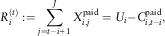 $$R_{i}^{{(t)}} :=\mathop{\sum}\limits_{j=t{\minus}i{\plus}1}^J X_{{i,j}}^{{{\rm paid}}} =U_{i} {\minus}C_{{i,t{\minus}i}}^{{{\rm paid}}}, $$
where  $$X_{{i,j}}^{{{\rm paid}}} $$
are the incremental claim payments of accident year i in development year j and
 $$C_{{i,t{\minus}i}}^{{{\rm paid}}} $$
the cumulative claim payments of accident year i until the end of calendar year t.
For claims reserving one has to predict these outstanding liabilities, which is equivalent to predicting the ultimate claim, that is
 $$\widehat{R}_{i}^{{(t)}} =\widehat{U}_{i}^{{(t)}} {\minus}C_{{i,t{\minus}i}}^{{{\rm paid}}}, $$
where  $$\widehat{U}_{i}^{{(t)}} $$
is a predictor of the ultimate claim U i at the end of calendar year t.
Best estimate reserves are reserves that are as accurate as possible and for best estimate reserves the expected value of the CDR is zero. In mathematical terms one has to be a bit more precise. Denote by  $${\cal A}_{t} $$
the σ-algebra containing all information available at time t. Best estimate reserves of accident year i at time t are then defined as the reserves minimising the conditional mean square error of prediction (msep):
 $${\rm msep}_{{\left. {R_{i}^{{(t)}} } \right|{\cal A}_{t} }} \left( {\widehat{R}_{i}^{{(t)}} } \right)=E\left[ {\left. {\left( {\widehat{R}_{i}^{{(t)}} {\minus}R_{i}^{{(t)}} } \right)^{2} } \right|{\cal A}_{t} } \right]$$
and are given by
 $$\widehat{R}_{i}^{{(t)}} =E\left[ {\left. {R_{i}^{{(t)}} } \right|{\cal A}_{t} } \right]=E\left[ {\left. {U_{i} } \right|{\cal A}_{t} } \right]{\minus}C_{{i,t{\minus}i}}^{{{\rm paid}}}. $$
The best estimate reserve at the end of calendar year t is then the sum over all accident years:
 $$\widehat{R}^{{(t)}} =\mathop{\sum}\limits_{i=t{\minus}J{\plus}1}^t \widehat{R}_{i}^{{(t)}}. $$
Remarks.
∙ The available information
 $${\cal A}_{t} $$
might consist of two components
$${\cal A}_{t} =\sigma \left( {{\cal D}_{t} ,{\cal I}_{t} } \right)$$
where
$${\cal D}_{t} $$
are the observed data until time t and where
$${\cal I}_{t} $$
denotes some additional external information, independent of the data such as observations and expert opinions with regard to legal and economic developments. In the actuarial literature often only the information contained in the data
$${\cal D}_{t} $$
is considered. However, we believe that additional available information should also be taken into account. In mathematical terms the sequences
$$\left\{ {{\cal A}_{t} :t=0,1,\,\ldots\,} \right\}$$
as well as
$$\left\{ {{\cal D}_{t} :t=0,1,\,\ldots\,} \right\}$$
and
$$\left\{ {{\cal I}_{t} :t=0,1,\,\ldots\,} \right\}$$
are filtrations.
∙
$$E\left[ {\left. {U_{i} } \right|{\cal A}_{t} } \right]$$
is not exactly known at time t, as it depends itself on unknown parameters. For instance, in the CL model of Mack (Reference Mack1993)
$$E\left[ {\left. {U_{i} } \right|{\cal A}_{t} } \right]$$
depends on the unknown CL factors f j, which have to be estimated from the data. Thus, to be strict, the best estimate reserve is only an estimate of the conditional expected value of the outstanding liabilities. However, we would like to study a model where best estimate reserves can explicitly be calculated in order to show that CDR’s with the same sign over several consecutive calendar years are not a contradiction to best estimate reserves. This means that even if we know the parameters exactly, CDR’s with the same sign over several consecutive calendar years are a phenomenon that is to be expected in certain situations. Therefore, it will be assumed that the best estimate reserves as defined in equation (2) are exactly known.


1.3. The martingale argument
The CDR of accident year t−J≤i≤t−1 in the financial statement of calendar year t is defined by
 $${\rm CDR}_{i}^{{(t)}} :=\widehat{R}_{i}^{{(t{\minus}1)}} {\minus}X_{{i,t{\minus}i}}^{{{\rm paid}}} {\minus}\widehat{R}_{i}^{{(t)}}, $$
where  $$X_{{i,t{\minus}i}}^{{{\rm paid}}} $$
denotes the incremental claim payments of accident year i in calendar year t. This can also be written as
 $${\rm CDR}_{i}^{{(t)}} =\widehat{U}_{i}^{{(t{\minus}1)}} {\minus}\widehat{U}_{i}^{{(t)}}. $$
Since
 $$\widehat{U}_{i}^{{(t)}} =E\left[ {\left. {U_{i} } \right|{\cal A}_{t} } \right],$$
the sequence
 $$\left\{ {\widehat{U}_{i}^{{(t)}} :t=i,i{\plus}1,\,\ldots\,} \right\}$$
is a martingale with respect to the filtration  $$({\cal A}_{t} )_{{t\in {\Bbb N}}} $$
. Hence the sequence
 $$\left\{ {{\rm CDR}_{i}^{{(t)}} :\;t=i{\plus}1,i{\plus}2,\,\ldots\,} \right\},$$
representing CDR’s in consecutive years, consists of increments of a martingale. Therefore, these CDR’s are uncorrelated and have expected value zero. From this fact it is often concluded that CDR’s having the same sign over several consecutive calendar years are a strong indication that the reserves are not best estimates.
Remark.
Also with a martingale it is not necessarily unlikely that the increments have the same sign over several consecutive years. This is, in particular, the case if the distribution of the CDR’s is strongly skewed to the left and if the probability of a positive CDR is much higher than 0.5. This can be the case in special lob such as product liability with potential large incurred but not reported claims occurring with a small probability. But even if the distribution is symmetric around zero and if we assume that CDR’s of different calendar years are independent, within a long-time horizon of say 50 years there is, for instance, a probability of 54.4% to have a consecutive period of 6 or more years with the same sign of the CDR. However, such long-time horizons are not considered in insurance, and for a reasonable time horizon of say 10 years this probability reduces to 9.4%. Thus, the martingale argument is not a very strict argument from a mathematical point of view but it reinforces the general belief, that CDR’s with the same sign over several consecutive years are a contradiction to best estimate reserves.
1.4. Observations in practice
In practice, however, one often observes the same sign of the CDR over several consecutive years. A striking example was the claims development after the mid-1990s in the line motor liability in Switzerland. Most of the Swiss insurance companies experienced a negative CDR over a longer period of about 8 consecutive years. The reason was the emergence of a new phenomenon called “whiplash”. It is mainly observed after rear-end collisions. The victims complain about permanent pain, chronic fatigue, loss of concentration and inability to work. However, as a peculiarity of this phenomenon, there is no objective medical injury that could be diagnosed by a medical doctor and that would explain these symptoms. Because of this lack of an observable medical indication the courts did not acknowledge a disability for such cases for a long time. But after a decision at the Swiss Federal court, the court practice began gradually to change. This was the beginning of a long process leading to a permanently increasing claims load, which was impossible to predict and that manifested itself only with time. For instance, there are many rear-end collisions, but fortunately most of them turned out to be harmless and only a small percentage developed to a case with long-term injury. However, at the beginning, there was no claims experience allowing to estimate neither this percentage nor the expected claim amount of the corresponding claims. There was also a change in the whole environment. For instance, more and more lawyers and law offices began to specialise on whiplash cases which itself increased the number of persons claiming for a disability. Or the advocates of the victims were not prepared to settle a claim in the hope that time works in favour of the victims and that they can get a higher amount at a later settlement date. It was also a cultural issue, as the whiplash phenomenon was mainly observed in the German speaking part of Switzerland and was practically non-existent in the French and Italian speaking part. The question was whether or when it would spill over to these parts of Switzerland, too. Fortunately it did not.
What are best reserve estimates in such periods of change and what should a reserving actuary do? We claim that it is not sufficient just to look at the claims triangle. In the paid claims triangle there is usually hardly seen any change at the early years of such a period and the new situation is reflected in the claims data only gradually and with a delay. In the incurred triangles one might observe an increase in the newer diagonals. However, such a new situation is also a challenge for the claims adjusters and there is a big uncertainty in their case estimates and as a consequence in the information observed in the newer diagonals of the incurred triangle. One of the authors has experienced other situations where the claims adjusters overreacted at the beginning. We claim that best practice is to communicate closely with the claims department, to take their judgement and evaluation as an expert opinion, which is permanently updated based on the development at the claims front (verdicts, court practice, etc.) and on the observed data in the claims triangles. In the motor liability example of the mid-1990s it took several years until the situation stabilised and the new court practice was reflected in the claims data, and hence the resulting CDR’s were negative over several years. In 2008, there was another decision at the Swiss Federal court with the effect that courts have become much more reluctant to attribute a permanent disability after an accident with whiplash indications. After that there was observed a similar development of the CDR’s in the opposite direction.
The Swiss motor liability example shows that also with best reserving practice the CDR’s can have the same sign over a longer period. The question arises whether we have overseen something in the martingale argument? The answer is yes, we have overseen something.
There is nothing wrong in the mathematics and the sequence  $$\{ \widehat{U}_{i}^{{(t)}} :t=i,i{\plus}1,\,\ldots\,\} $$
, as defined in equation (4), is a martingale. However, one has to be careful in the interpretation what this martingale property exactly means and what conclusions one can draw from the martingale argument. The point is that the claim payments and the claims development depend on “hidden”, not directly observable, characteristics describing the “state space” at different times such as legal and economic environment. These “hidden” characteristics are best modelled in a Bayesian way as random variables. The martingale argument only holds in the average over these state space characteristics. But what we observe in a claims development triangle are conditional observations, that is, claims data generated on the condition that a specific but unknown realisation of the state space variables is given. The observed CDR’s resulting from best estimates based on such conditional observations are no longer increments of a martingale with expected value zero. This fact will become more clear when looking at some concrete examples.
2. An example from pricing
The Poisson-Gamma model is a well-known model for experience rating based on observed claim frequencies and was for instance the basis for constructing the Bonus-Malus scheme in motor liability in Switzerland (see Bichsel, Reference Bichsel1964).
Assume we have a portfolio of risks numbered i=1,2, …, I and denote by N i,j the claim number of risk i in year j. Each risk is characterised by its risk characteristic ϑ i which is a realisation of a random variable Θi.
Model Assumptions 2.1 (Poisson-Gamma) i) Conditionally, given Θi=ϑ i, the random variables N i,j (j=1,2, …) are independent and Poisson distributed with Poisson parameter ϑ iλ 0.
ii) The random variables Θiare independent and Gamma distributed with E[Θi]=1 and Var(Θi)=γ −1.
iii) N i,jand N k,lare independent for i ≠ k.
Denote by  $${\cal D}_{t} =\left\{ {N_{{i,j}} :j=1,2,\,\ldots\,,t;i=1,2,\,\ldots\,,I} \right\}$$
the observations up to year t. Based on these observed data we want to predict for each risk i next years claim number. The following theorem is well-known from credibility literature (see, for instance, Bühlmann & Gisler, Reference Bühlmann and Gisler2005, Chapter 2).
Theorem 2.2 The best prediction of N i,t+1given  $${\cal D}_{t} $$
under Model Assumptions 2.1 is given by
 $$\widehat{N}_{{i,t{\plus}1}} =\alpha _{t} \bar{N}_{{i,t}} {\plus}(1{\minus}\alpha _{t} )\lambda _{0}, $$
where
 $$\bar{N}_{{i,t}} ={1 \over t}\mathop{\sum}\limits_{j=1}^t N_{{i,j}} \quad {\rm and}\quad \alpha _{t} ={{t\lambda _{0} } \over {t\lambda _{0} {\plus}\gamma }}.$$
Remarks.
∙ The individual risk characteristics ϑ i are drawn at the very beginning from a first “urn” as realisations of independent and identically distributed Gamma random variables.
∙ The sequence
$$\left\{ {\widehat{N}_{{i,t}} :\;t=1,2,\,\ldots\,} \right\}$$
is a martingale with respect to
$$({\cal D}_{t} )_{{t\in {\Bbb N}}} $$
and it holds that (5)
$$E\left[ {\left. {\widehat{N}_{{i,t{\plus}1}} {\minus}N_{{i,t{\plus}1}} } \right|N_{{i,1}} ,\,\ldots\,,N_{{i,t}} } \right]=0.$$
This means that for an infinitely large portfolio there is a balance between forecasted and future claim frequency in all sub-portfolios of drivers having the same claim experience N i,1, …, N i,t. This is the best we can achieve for a risk-adjusted pricing. However, the left-hand side of equation (5) is an expected value over the whole Θ space.
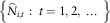
∙ But the martingale property does not hold for the observations of a specific driver i. A specific driver i has its specific risk characteristics Θi=ϑ i drawn from a first urn, and the observed claim numbers N i,j of this particular driver are independent and Poisson distributed with Poisson parameter ϑ iλ 0. We then have


 $$\eqalignno{ E\left[ {\left. {\widehat{N}_{{i,t{\plus}1}} {\minus}N_{{i,t{\plus}1}} } \right|N_{{i,1}} ,\,\ldots\,,N_{{i,t}} ,\Theta _{i} } \right]= & \widehat{N}_{{i,t{\plus}1}} {\minus}E\left[ {\left. {N_{{i,t{\plus}1}} } \right|\Theta _{i} } \right] \cr = & \alpha _{t} \left( {\bar{N}_{{i,t}} {\minus}\lambda _{0} } \right){\plus}\lambda _{0} \left( {1{\minus}\Theta _{i} } \right), $$
which is in general different from zero. Moreover,
 $$\eqalignno{ E\left[ {\left. {\widehat{N}_{{i,t{\plus}1}} {\minus}N_{{i,t{\plus}1}} } \right|\Theta _{i} } \right]= \,& \alpha _{t} \left( {\lambda _{0} \Theta _{i} {\minus}\lambda _{0} } \right){\plus}\lambda _{0} \left( {1{\minus}\Theta _{i} } \right) \cr = \,& \lambda _{0} \left( {1{\minus}\alpha _{t} } \right)\left( {1{\minus}\Theta _{i} } \right). $$
Thus, our best estimate predictor has conditional on Θi an upward (Θi<1) or downward (Θi>1) bias for all years t. This bias decreases when the observed number t of years increases.
In reserving we do not have a portfolio of different similar claims triangles and we are not interested in the mean over these triangles. We are rather looking at one specific triangle with given hidden state space characteristics comparable to a specific driver in the pricing example. Conditional on this hidden risk characteristics the best estimate reserves are no longer unbiased, and this bias can have the same sign over several consecutive calendar years. If the 1-year process variance is small compared to this bias, we will observe a CDR with the same sign over several consecutive years. In section 3 we will consider examples from reserving.
3. Examples from reserving
3.1. Basic Bayesian framework
It is our personal belief, based on many years of practical experience of one of the authors, that reserving is as much art as science. By this we mean that a good reserving actuary in practice should not only analyse claims data from a claims triangle. There is much more information available which one could and should take into account. The lawyers and claims adjusters in the company will have some knowledge about changes in legislation, about claims handling, claims processes and the assessment of case estimates by the claims adjusters. Economists will have some opinion about the future development of economic factors. In short, there is a lot of expert knowledge available in a company from which one can learn something about the expected future claim payments. Beside the data in the triangle this expert knowledge should also be taken into account when calculating best estimate claims reserves.
In mathematical terms such a situation can best be modelled in a Bayesian framework, which is predestinated to deal with a priori knowledge on the one hand and observed claims data on the other. In such a framework the best estimate reserve is given by equation (2). Often there is no explicit formula for equation (2) and in this case a good approximation could be to use credibility theory instead. There is one difference to the credibility models usually considered in the literature: the a priori information does also change in time. In suitable models this can still be handled by recursive estimators.
The basic Bayesian framework considered in this paper is a multiplicative model with the Bayesian structure given below in Model Assumptions 3.1. Recall that  $${\cal I}_{t} $$
denotes the external information at time t and
 $${\cal D}_{t} $$
is defined as in equation (1). By calendar year effect we mean that
 $$E\left[ {\left. {X_{{i,j}} } \right|\Psi ,{\cal I}_{t} } \right]=E\left[ {\left. {X_{{i,j}} } \right|\Psi _{{i{\plus}j}} } \right]=\mu _{i} \gamma _{j} \Psi _{{i{\plus}j}} ,\quad t\geq 0.$$
Since the Ψt are multiplicative factors to be applied on the conditional expected value of all elements of a diagonal, they are also called diagonal effects. We denote by Ψ={Ψ0,Ψ1, …} the set of diagonal effects in all calendar years  $$t\in {\Bbb N}$$
.
Model Assumptions 3.1 (Bayes Model with Diagonal Effects) Conditionally, given Ψand  $${\cal I}_{t} $$
for any t≥0, the increments X i,jare independent and there exist constants μ i, 0≤i≤t, and γ j, 0≤j≤J, with ∑jγ j=1 such that
 $$E\left[ {X_{{i,j}} {\rm \,\mid\,}\Psi ,{\cal I}_{t} } \right]=\mu _{i} \gamma _{j} \Psi _{{i{\plus}j}}. $$
Here {γ j, j=0, …, J} is the incremental payment pattern and {β j, j=0, …, J} with  $$\beta _{j} =\mathop{\sum}\nolimits_{k=0}^j \gamma _{k} $$
the cumulative payment pattern.
Remark.
If Ψt=1 for all t≥0, then there are no calendar year effects and if we omit the external information  $${\cal I}_{t} $$
in Model Assumptions 3.1 we obtain the basic assumptions of the Bornhuetter–Ferguson (BF) model (see, for instance, Wüthrich & Merz, Reference Wüthrich and Merz2008). The best estimate reserve for accident year i at time t is then given by
 $$\widehat{R}_{i} =\left( {1{\minus}\beta _{{t{\minus}i}} } \right)\mu _{i} $$
which is the BF reserve formula.
Under Model Assumptions 3.1 the best estimate reserve of accident year i at the end of calendar year t is given by
 $$\eqalignno{ \widehat{R}_{i}^{{(t)}} = & E\left[ {\left. {R_{i} } \right|{\cal I}_{t} ,{\cal D}_{t} } \right]=E\left[ {\left. {E\left[ {\left. {R_{i} } \right|{\cal I}_{t} ,{\cal D}_{t} ,\Psi } \right]} \right|{\cal I}_{t} ,{\cal D}_{t} } \right] \cr = & \mu _{i} \mathop{\sum}\limits_{j=t{\minus}i{\plus}1}^J \gamma _{j} E\left[ {\left. {\Psi _{{i{\plus}j}} } \right|{\cal I}_{t} ,{\cal D}_{t} } \right], $$
and the best estimate of the total reserve at the end of calendar year t is
 $$\eqalignno{ \widehat{R}^{{(t)}} = & \mathop{\sum}\limits_{i=t{\minus}J{\plus}1}^t \widehat{R}_{i}^{{(t)}} \cr = & \mathop{\sum}\limits_{i=t{\minus}J{\plus}1}^t \mu _{i} \:\mathop{\sum}\limits_{j=t{\minus}i{\plus}1}^J \gamma _{j} E\left[ {\left. {\Psi _{{i{\plus}j}} } \right|{\cal I}_{t} ,{\cal D}_{t} } \right] \cr = & \mathop{\sum}\limits_{k=1}^J \left( {E\left[ {\left. {\Psi _{{t{\plus}k}} } \right|{\cal I}_{t} ,{\cal D}_{t} } \right]\mathop{\sum}\limits_{j=k}^J \gamma _{j} \mu _{{t{\plus}k{\minus}j}} } \right). $$
Hence to find the best estimate reserve  $$\widehat{R}^{{(t)}} $$
we have to determine
 $$\Psi _{{t{\plus}k}}^{{\left( t \right)}} =E\left[ {\left. {\Psi _{{t{\plus}k}} } \right|{\cal I}_{t} ,{\cal D}_{t} } \right]$$
for k=1, …, J. Note that  $$\Psi _{{t{\plus}k}}^{{\left( t \right)}} $$
is the best k-year prediction of Ψt+k at time t.
One year later there are the observations of the diagonal of the next calendar year t+1 and possibly updated external information  $${\cal I}_{{t{\plus}1}} $$
available. With these new informations we get the updated forecasts of
 $$\Psi _{{t{\plus}k}}^{{\left( {t{\plus}1} \right)}} $$
.
From equation (7) it follows that the total CDR in calendar year t+1 is given by
 $$\eqalignno{ {\rm CDR}_{{t{\plus}1}} = & E\left[ {\left. {\mathop{\sum}\limits_{i=0}^t U_{i} } \right|{\cal I}_{t} ,{\cal D}_{t} } \right]{\minus}E\left[ {\left. {\mathop{\sum}\limits_{i=0}^t U_{i} } \right|{\cal I}_{{t{\plus}1}} ,{\cal D}_{{t{\plus}1}} } \right] \cr = & \mathop{\sum}\limits_{i=t{\minus}J{\plus}1}^t \mu _{i} \mathop{\sum}\limits_{j=t{\minus}i{\plus}1}^J \gamma _{j} \Psi _{{i{\plus}j}}^{{(t)}} {\minus}\mathop{\sum}\limits_{i=t{\minus}J{\plus}1}^t X_{{i,t{\minus}i{\plus}1}} {\minus}\mathop{\sum}\limits_{i=t{\minus}J{\plus}2}^t \mu _{i} \mathop{\sum}\limits_{j=t{\minus}i{\plus}2}^J \gamma _{j} \Psi _{{i{\plus}j}}^{{(t{\plus}1)}} \cr = & \mathop{\sum}\limits_{k=t{\plus}1}^{t{\plus}J} \Psi _{k}^{{(t)}} \mathop{\sum}\limits_{j=k{\minus}t}^J \mu _{{k{\minus}j}} \gamma _{j} {\minus}\mathop{\sum}\limits_{j=1}^J X_{{t{\plus}1{\minus}j,j}} {\minus}\mathop{\sum}\limits_{k=t{\plus}2}^{t{\plus}J} \Psi _{k}^{{(t{\plus}1)}} \mathop{\sum}\limits_{j=k{\minus}t}^J \mu _{{k{\minus}j}} \gamma _{j} \cr = & \mathop{\sum}\limits_{l=1}^J \Psi _{{t{\plus}l}}^{{(t)}} \mathop{\sum}\limits_{j=l}^J \mu _{{t{\plus}l{\minus}j}} \gamma _{j} {\minus}\mathop{\sum}\limits_{j=1}^J X_{{t{\plus}1{\minus}j,j}} {\minus}\mathop{\sum}\limits_{l=2}^J \Psi _{{t{\plus}l}}^{{(t{\plus}1)}} \mathop{\sum}\limits_{j=l}^J \mu _{{t{\plus}l{\minus}j}} \gamma _{j}. $$
In the special case where μ i=μ for all i, equations (7) and (8) simplify to
 $$\widehat{R}^{{(t)}} =\mu \mathop{\sum}\limits_{k=1}^J \Psi _{{t{\plus}k}}^{{(t)}} (1{\minus}\beta _{{k{\minus}1}} ),$$
 $${\rm CDR}_{{t{\plus}1}} = & \mathop{\underbrace{{\Psi _{{t{\plus}1}}^{{(t{\plus}1)}} \mu (1{\minus}\beta _{0} ){\minus}\mathop{\sum}\limits_{j=1}^J X_{{t{\plus}1{\minus}j,j}} }}}\limits_{{\rm difference}\,{\rm between}\,{\rm updated}\,{\rm forecast}\,{\rm and}\,{\rm observations}}{\plus}\mathop{\underbrace{{\mathop{\sum}\limits_{k=1}^J \left( {\Psi _{{t{\plus}k}}^{{(t)}} {\minus}\Psi _{{t{\plus}k}}^{{(t{\plus}1)}} } \right)\mu (1{\minus}\beta _{{k{\minus}1}} )}}}\limits_{{\rm change}\,{\rm in}\,{\rm update}}$$
 $$= & \mathop{\underbrace{{\Psi _{{t{\plus}1}}^{{(t)}} \mu (1{\minus}\beta _{0} ){\minus}\mathop{\sum}\limits_{j=1}^J X_{{t{\plus}1{\minus}j,j}} }}}\limits_{{\rm difference}\,{\rm between}\,{\rm forecast}\,{\rm and}\,{\rm observations}}{\plus}\mathop{\underbrace{{\mathop{\sum}\limits_{k=2}^J \left( {\Psi _{{t{\plus}k}}^{{(t)}} {\minus}\Psi _{{t{\plus}k}}^{{(t{\plus}1)}} } \right)\mu (1{\minus}\beta _{{k{\minus}1}} )}}}\limits_{{\rm change}\,{\rm future}}.$$
In the following we consider two specific models within this basic Bayesian framework in which we can explicitly calculate best estimate reserves.
3.2. One Jump Model
We consider the simple situation with a stable period in the years t≤s 0−1 with no diagonal effects observable in the claims triangles and with no indication that this situation will change in the future. However, in the year s 0, there is a change in the environment (e.g. legislation), which leads to a change of the expected value of the total claim payments in each “cell” {(i,j): i+j≥s 0} by some unknown factor  $$\Psi _{{s_{0} }} $$
. There is no indication that further changes will incur after year s 0. After calendar year s 0 the situation is again stable. This situation is reflected by the following model.
Model Assumptions 3.2 (One Jump Model) i) Conditionally, given Ψand  $${\cal I}_{t} $$
for any t≥0, the X i,jare independent and normally distributed with
 $$E[X_{{i,j}} {\rm \,\mid\,}\Psi ,{\cal I}_{t} ]=\mu _{i} \gamma _{j} \Psi _{{i{\plus}j}} ,\quad {\rm Var}(X_{{i,j}} {\rm \,\mid\,}\Psi ,{\cal I}_{t} )=\mu _{i} \eta _{j}^{2} \sigma ^{2}, $$
where  $\mathop{\sum}\nolimits_{j=0}^J {\gamma _{j} } =\mathop{\sum}\nolimits_{j=0}^J {\eta _{j}^{2} =1.} $
ii) For t≤s 0−1, conditionally on  $${\cal I}_{t} $$
and
 $${\cal D}_{t} $$
, Ψl=1 for l≤t and
 $$E[\Psi _{{t{\plus}l}} {\rm \,\mid\,}{\cal I}_{t} ,{\cal D}_{t} ]=1,\quad l\geq 1.$$
iii) For t≥s 0, conditionally, given  $${\cal I}_{t} $$
and
 $${\cal D}_{{t{\minus}1}} $$
 $$\eqalignno{ \Psi _{l} = & 1,\quad l\leq s_{0} {\minus}1, \cr \Psi _{l} = & \Psi _{{s_{0} }} ,\quad s_{0} \leq l\leq t, \cr E[\Psi _{{t{\plus}l}} {\rm \,\mid\,}{\cal I}_{t} ,{\cal D}_{t} ]= & E[\Psi _{{s_{0} }} {\rm \,\mid\,}{\cal I}_{t} ,{\cal D}_{t} ],\quad l\geq 0, $$
where  $$\Psi _{{s_{{_{0} }} }} {\rm\! \mid}({\cal I}_{t} ,{\cal D}_{{s_{{_{0} }} {\minus}1}} )\mathop{=}\limits^{d} \Psi _{{s_{{_{0} }} }} {\rm \! \mid}({\cal I}_{{s_{{_{0} }} }} ,{\cal D}_{{s_{{_{0} }} {\minus}1}} )\,\sim\,N(m,\tau ^{2} )$$
.
Remarks.
∙ The stable situation without diagonal effect in the period t≤s 0−1 and no indication for a change in the future is modelled by ii) (Ψl=1 for l≤t and prediction
$$E[\Psi _{{t{\plus}l}} {\rm \,\mid\,}{\cal I}_{t} ,{\cal D}_{t} ]=1$$
for future years).∙ The change of future payments by an unknown factor due to the change of the environment in the year s 0 is modelled by
$$\Psi _{{s_{0} }} {\rm \,\mid\,}({\cal I}_{{s_{0} }} ,{\cal D}_{{s_{0} {\minus}1}} )\,\sim\,N(m,\tau ^{2} )$$
in iii). Note that this means a change of the “expert opinion” with regard to the years t≥s 0.∙ The stable situation with no further changes after the year s 0 is modelled by
$$\Psi _{{s_{0} }} {\rm \,\mid\,}({\cal I}_{t} ,{\cal D}_{{s_{0} {\minus}1}} )\mathop{=}\limits^{d} \Psi _{{s_{0} }} {\rm \,\mid\,}({\cal I}_{{s_{0} }} ,{\cal D}_{{s_{0} {\minus}1}} )$$
and the fact that there is no indication for a change in the future by
$$E[\Psi _{{t{\plus}l}} {\rm \,\mid\,}{\cal I}_{t} ,{\cal D}_{t} ]=E[\Psi _{{s_{0} }} {\rm \,\mid\,}{\cal I}_{t} ,{\cal D}_{t} ]$$
for l≥0.




In order to simplify the formulas we assume in the following that s 0≥J.
Proposition 3.3 Under Model Assumptions 3.2  $$\Psi _{{s_{0} }} $$
is conditioned on
 $${\cal D}_{{s_{0} {\plus}l}} $$
and
 $${\cal I}_{{s_{0} {\plus}l}} $$
, l≥0, normally distributed with
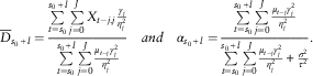
 $$\eqalignno{ \Psi _{{s_{0} }}^{{(s_{{_{0} }} {\plus}l)}} = & E[\Psi _{{s_{0} }} {\rm \,\mid\,}{\cal I}_{{s_{0} {\plus}l}} ,{\cal D}_{{s_{0} {\plus}l}} ]=\alpha _{{s_{0} {\plus}l}} \bar{D}_{{s_{0} {\plus}l}} {\plus}(1{\minus}\alpha _{{s_{0} {\plus}l}} )m, \cr q_{{s_{0} }}^{{(s_{0} {\plus}l)}} = & {\rm Var}(\Psi _{{s_{0} }} {\rm \,\mid\,}{\cal I}_{{s_{0} {\plus}l}} ,{\cal D}_{{s_{0} {\plus}l}} )=(1{\minus}\alpha _{{s_{0} {\plus}l}} )\tau ^{2}, $$
where
 $$\bar{D}_{{s_{0} {\plus}l}} ={{\mathop{\sum}\limits_{t=s_{0} }^{s_{0} {\plus}l} \mathop{\sum}\limits_{j=0}^J X_{{t{\minus}j,j}} {{\gamma _{j} } \over {\eta _{j}^{2} }}} \over {\mathop{\sum}\limits_{t=s_{0} }^{s_{0} {\plus}l} \mathop{\sum}\limits_{j=0}^J {{\mu _{{t{\minus}j}} \gamma _{j}^{2} } \over {\eta _{j}^{2} }}}}\quad and\quad \alpha _{{s_{0} {\plus}l}} ={{\mathop{\sum}\limits_{t=s_{0} }^{s_{0} {\plus}l} \mathop{\sum}\limits_{j=0}^J {{\mu _{{t{\minus}j}} \gamma _{j}^{2} } \over {\eta _{j}^{2} }}} \over {\mathop{\sum}\limits_{t=s_{0} }^{s_{0} {\plus}l} \mathop{\sum}\limits_{j=0}^J {{\mu _{{t{\minus}j}} \gamma _{j}^{2} } \over {\eta _{j}^{2} }}{\plus}{{\sigma ^{2} } \over {\tau ^{2} }}}}.$$
Remark.
Proposition 3.3 still yields the credibility estimator if we drop the normality assumption for  $$\Psi _{{s_{0} }} $$
and the X i,j. In a distribution-free approach, it is the best linear approximation to the Bayes estimator and in this sense still a best estimate. However, it is then no longer exact Bayesian and a best estimate as defined in equation (2).
Proof of Proposition 3.3:
In the One Jump Model 3.2 we have exact credibility, that is, the credibility estimator is exact Bayesian (see, e.g. Jewell, Reference Jewell1974a, Reference Jewell1974b or Bühlmann & Gisler, Reference Bühlmann and Gisler2005). If γ j ≠ 0 for j=0, …, J, then the random variables
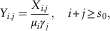 $$Y_{{i,j}} ={{X_{{i,j}} } \over {\mu _{i} \gamma _{j} }},\quad i{\plus}j\geq s_{0}, $$
fulfil the assumptions of the Bühlmann–Straub model with weights w i,j=μ iγ j2/(σ 2η j2). The formula then follows from the Bühlmann–Straub credibility formula. For incurred claims some of the γ j might be zero. The formula can then be derived with the regression credibility model (see Theorem 8.4 in Bühlmann & Gisler, Reference Bühlmann and Gisler2005) by using the observation vector  $$X^{{(s_{0} {\plus}l)}} $$
with all observations from calendar year s 0 to calendar year s 0+l as elements, where the regression equation is given by
 $$E[X_{{i,j}} {\rm \,\mid\,}\Psi _{{s_{0} }} ]=\mu _{i} \gamma _{j} \Psi _{{s_{0} }} $$
and where the conditional covariance matrix of
 $$X^{{(s_{0} {\plus}l)}} $$
given
 $$\Psi _{{s_{0} }} $$
is diagonal with diagonal elements
 $${\rm Var}(X_{{i,j}} {\rm \,\mid\,}\Psi _{{s_{0} }} )=\mu _{i} \eta _{j}^{2} \sigma ^{2} $$
.
The predictors  $$\Psi _{{s_{0} }}^{{(t)}} $$
and the variances
 $$q_{{s_{0} }}^{{(t)}} $$
can also be calculated recursively (see Theorem 9.6 in Bühlmann & Gisler, Reference Bühlmann and Gisler2005):
Proposition 3.4 We have the following recursive formulas:
i) For t≤s 0−1
 $$\Psi _{{s_{0} }}^{{(t)}} =1.$$
ii) For t=s 0
 $$\Psi _{{s_{0} }}^{{(s_{0} )}} =\tilde{\alpha }_{{s_{0} }} {{\mathop{\sum}\limits_{j=0}^J X_{{s_{0} {\minus}j,j}} {{\gamma _{j} } \over {\eta _{j}^{2} }}} \over {w_{{s_{0} }} }}{\plus}(1{\minus}\tilde{\alpha }_{{s_{0} }} )m,\quad q_{{s_{0} }}^{{(s_{0} )}} =(1{\minus}\tilde{\alpha }_{{s_{0} }} )\tau ^{2}, $$
where
 $$\tilde{\alpha }_{{s_{0} }} ={{w_{{s_{0} }} } \over {w_{{s_{0} }} {\plus}{{\sigma ^{2} } \over {\tau ^{2} }}}}\quad and\quad w_{{s_{0} }} =\mathop{\sum}\limits_{j=0}^J \mu _{{s_{0} {\minus}j}} {{\gamma _{j}^{2} } \over {\eta _{j}^{2} }}.$$
iii) For t>s 0
 $$\Psi _{{s_{0} }}^{{(t)}} =\tilde{\alpha }_{t} {{\mathop{\sum}\limits_{j=0}^J X_{{t{\minus}j,j}} {{\gamma _{j} } \over {\eta _{j}^{2} }}} \over {w_{t} }}{\plus}(1{\minus}\tilde{\alpha }_{t} )\Psi _{{s_{0} }}^{{(t{\minus}1)}} ,\quad q_{{s_{0} }}^{{(t)}} =(1{\minus}\tilde{\alpha }_{t} )q_{{s_{0} }}^{{(t{\minus}1)}} ,$$
where
 $$\tilde{\alpha }_{t} ={{w_{t} } \over {w_{t} {\plus}{{\sigma ^{2} } \over {q_{{s_{0} }}^{{(t{\minus}1)}} }}}}\quad and\quad w_{t} =\mathop{\sum}\limits_{j=0}^J \mu _{{t{\minus}j}} {{\gamma _{j}^{2} } \over {\eta _{j}^{2} }}.$$
With Proposition 3.4 we can also find an explicit formula for the CDR. For simplicity we consider the case with μ i ≡ μ. By using equations (9) and (10) we obtain:
∙ for  $$t{\plus}1\leq s_{0} {\minus}1$$
 $$\eqalignno{ {\rm CDR}_{{t{\plus}1}}=\ & \mu (1{\minus}\beta _{0} ){\minus}\mathop{\sum}\limits_{j=1}^J X_{{t{\plus}1{\minus}j,j}} \cr = & \, {\rm difference}\,{\rm between}\,{\rm forecast}\,{\rm and}\,{\rm observations}, $$
∙ for  $$t{\plus}1=s_{0} $$
 $$\eqalignno{ {\rm CDR}_{{s_{0} }} = & \mathop{\underbrace{{\Psi _{{s_{0} }}^{{(s_{0} )}} \mu (1{\minus}\beta _{0} ){\minus}\mathop{\sum}\limits_{j=1}^J X_{{s_{0} {\minus}j,j}} }}}\limits_{{\rm difference}\,{\rm between}\,{\rm updated}\,{\rm forecast}\,{\rm and}\,{\rm observations}}{\plus}\mathop{\underbrace{{\left( {1{\minus}\Psi _{{s_{0} }}^{{(s_{0} )}} } \right)\mu \mathop{\sum}\limits_{k=1}^J (1{\minus}\beta _{{k{\minus}1}} )}}}\limits_{{\rm change}\,{\rm in}\,{\rm update}} \cr =\mathop{\underbrace{{\mu (1{\minus}\beta _{0} ){\minus}\mathop{\sum}\limits_{j=1}^J X_{{s_{0} {\minus}j,j}} }}}\limits_{{\rm difference}\,{\rm between}\,{\rm forecast}\,{\rm and}\,{\rm observations}}{\plus}\mathop{\underbrace{{\left( {1{\minus}\Psi _{{s_{0} }}^{{(s_{0} )}} } \right)\mu \mathop{\sum}\limits_{k=2}^J (1{\minus}\beta _{{k{\minus}1}} )}}}\limits_{{\rm change}\,{\rm future}}, \cr $$
and
 $$1{\minus}\Psi _{{s_{0} }}^{{(s_{0} )}} = & 1{\minus}m{\plus}\tilde{\alpha }_{{s_{0} }} \left( {m{\minus}{{\mathop{\sum}\limits_{j=0}^J X_{{s_{0} {\minus}j,j}} {{\gamma _{j} } \over {\eta _{j}^{2} }}} \over {w_{{s_{0} }} }}} \right)\!,$$
∙ for  $$t{\plus}1\gt s_{0} $$
 $$\eqalignno{ {\rm CDR}_{{t{\plus}1}} = & \mathop{\underbrace{{\Psi _{{s_{0} }}^{{(t{\plus}1)}} \mu (1{\minus}\beta _{0} ){\minus}\mathop{\sum}\limits_{j=1}^J X_{{t{\plus}1{\minus}j,j}} }}}\limits_{{\rm difference}\,{\rm between}\,{\rm updated}\,{\rm forecast}\,{\rm and}\,{\rm observations}}{\plus}\mathop{\underbrace{{\left( {\Psi _{{s_{0} }}^{{(t)}} {\minus}\Psi _{{s_{0} }}^{{(t{\plus}1)}} } \right)\mu \mathop{\sum}\limits_{k=1}^J (1{\minus}\beta _{{k{\minus}1}} )}}}\limits_{{\rm change}\,{\rm in}\,{\rm update}} \cr = & \mathop{\underbrace{{\Psi _{{s_{0} }}^{{(t)}} \mu (1{\minus}\beta _{0} ){\minus}\mathop{\sum}\limits_{j=1}^J X_{{t{\plus}1{\minus}j,j}} }}}\limits_{{\rm difference}\,{\rm between}\,{\rm forecast}\,{\rm and}\,{\rm observations}}{\plus}\mathop{\underbrace{{\left( {\Psi _{{s_{0} }}^{{(t)}} {\minus}\Psi _{{s_{0} }}^{{(t{\plus}1)}} } \right)\mu \mathop{\sum}\limits_{k=2}^J (1{\minus}\beta _{{k{\minus}1}} )}}}\limits_{{\rm change}\,{\rm future}}, $$
and
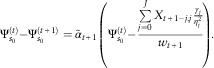 $$\Psi _{{s_{0} }}^{{(t)}} {\minus}\Psi _{{s_{0} }}^{{(t{\plus}1)}} =\tilde{\alpha }_{{t{\plus}1}} \left( {\Psi _{{s_{0} }}^{{(t)}} {\minus}{{\mathop{\sum}\limits_{j=0}^J X_{{t{\plus}1{\minus}j,j}} {{\gamma _{j} } \over {\eta _{j}^{2} }}} \over {w_{{t{\plus}1}} }}} \right)\!.$$
We observe that in the case t+1>s 0 the second terms “change in update” and “change future” respectively, converge to 0 as t→∞ since the weights  $$\tilde{\alpha }_{{t{\plus}1}} \to0$$
. On the other hand, the difference between (updated) forecast and observations depends more on the volatility of the data.
Next, we want to consider the sign of the CDR over several consecutive calendar years in the period starting at year s 0+1. What we will observe are conditional data generated by the model, given a specific realisation of  $$\Psi _{{s_{0} }}^{{}} $$
. For this reason we first investigate the behaviour of the conditional expected value
 $$E[\Psi _{{s_{0} }}^{{(t)}} {\rm \,\mid\,}{\cal I}_{{s_{0} }} ,{\cal D}_{{s_{0} {\minus}1}} ,\Psi _{{s_{0} }} ]$$
.
With the estimator  $$\Psi _{{s_{0} }}^{{(t)}} $$
in Proposition 3.3 and from
 $$E[\bar{D}_{t} {\rm \,\mid\,}{\cal I}_{{s_{0} }} ,{\cal D}_{{s_{0} {\minus}1}} ,\Psi _{{s_{0} }} ]=\Psi _{{s_{0} }} $$
, t≥s 0, it follows that
 $$E\left[ {\left. {\Psi _{{s_{0} }}^{{(t)}} {\minus}\Psi _{{s_{0} }}^{{(t{\plus}1)}} } \right|{\cal I}_{{s_{0} }} ,{\cal D}_{{s_{0} {\minus}1}} ,\Psi _{{s_{0} }} } \right]=(\alpha _{t} {\minus}\alpha _{{t{\plus}1}} )(\Psi _{{s_{0} }} {\minus}m).$$
We then obtain for the conditional expectation of the CDR for t+1>s 0:
 $$\hskip-26.3pcE\left[ {{\rm CDR}_{{t{\plus}1}}\!\! \mid \!{\cal I}_{{s_{0} }} ,{\cal D}_{{s_{0} {\minus}1}} ,\Psi _{{s_{0} }} } \right]$$
 $$\eqalignno{ \quad\quad\quad\quad =\ & \mu (1{\minus}\beta _{0} )(1{\minus}\alpha _{t} )(m{\minus}\Psi _{{s_{0} }} ){\plus}E\left[ {\left. {\Psi _{{s_{0} }}^{{(t)}} {\minus}\Psi _{{s_{0} }}^{{(t{\plus}1)}} } \right|{\cal I}_{{s_{0} }} ,{\cal D}_{{s_{0} {\minus}1}} ,\Psi _{{s_{0} }} } \right]\mu \mathop{\sum}\limits_{k=2}^J (1{\minus}\beta _{{k{\minus}1}} ) \cr \quad =\, & \mu (1{\minus}\beta _{0} )(1{\minus}\alpha _{t} )(m{\minus}\Psi _{{s_{0} }} ){\plus}(\alpha _{{t{\plus}1}} {\minus}\alpha _{t} )\left( {m{\minus}\Psi _{{s_{0} }} } \right)\mu \mathop{\sum}\limits_{k=2}^J (1{\minus}\beta _{{k{\minus}1}} ) \cr \quad = \,& (m{\minus}\Psi _{{s_{0} }} )\mu \left( {(1{\minus}\beta _{0} )(1{\minus}\alpha _{t} ){\plus}(\alpha _{{t{\plus}1}} {\minus}\alpha _{t} )\mathop{\sum}\limits_{k=2}^J (1{\minus}\beta _{{k{\minus}1}} )} \right). $$
If β j≤1 for all j, or γ j≥0 for all j, respectively, then the second factor in equation (11) is positive since α t is increasing in t. Moreover, this second factor decreases in t since 1−α t and α t+1−α t are decreasing. In the limit for t→∞, it vanishes. In addition, we can see from equation (11) that the absolute value of the conditional expectation of the CDR is larger if more weight is given to the tail, that is, for long-tailed lob the bias is higher.
Hence, we have found the following result with regard to the behaviour of the conditional expected value of the CDR in the case where γ j≥0 for all j:
∙ The sign of
$$E\left[ {{\rm CDR}_{{t{\plus}1}} {\rm \,\mid\,}{\cal I}_{{s_{0} }} ,{\cal D}_{{s_{0} {\minus}1}} ,\Psi _{{s_{0} }} } \right]$$
is the same for all t+1≥s 0+1.∙ The absolute value of
$$E\left[ {{\rm CDR}_{{t{\plus}1}} {\rm \,\mid\,}{\cal I}_{{s_{0} }} ,{\cal D}_{{s_{0} {\minus}1}} ,\Psi _{{s_{0} }} } \right]$$
is the bigger, the bigger
$$\,\mid\,m{\minus}\Psi _{{s_{0} }} \,\mid\,$$
is.∙ The absolute value of
$$E\left[ {{\rm CDR}_{{t{\plus}1}} {\rm \,\mid\,}{\cal I}_{{s_{0} }} ,{\cal D}_{{s_{0} {\minus}1}} ,\Psi _{{s_{0} }} } \right]$$
is the bigger, the longer the development is. In other words, the absolute value of
$$E\left[ {{\rm CDR}_{{t{\plus}1}} {\rm \,\mid\,}{\cal I}_{{s_{0} }} ,{\cal D}_{{s_{0} {\minus}1}} ,\Psi _{{s_{0} }} } \right]$$
is bigger, if the development pattern (β j)0≤j≤J increases slower to β J=1.∙ The absolute value of
$$E\left[ {{\rm CDR}_{{t{\plus}1}} {\rm \,\mid\,}{\cal I}_{{s_{0} }} ,{\cal D}_{{s_{0} {\minus}1}} ,\Psi _{{s_{0} }} } \right]$$
is decreasing in t.∙ In the limit for t→∞ the CDR is conditionally unbiased.


3.2.1. Numerical example
For the example we choose a special case of the above model in which μ i ≡ μ and η j2=γ j. In this case the formula for  $$\Psi _{{s_{0} }}^{{(t)}} $$
simplifies to
 $$\Psi _{{s_{0} }}^{{(t)}} =\alpha _{t} {1 \over {\mu (t{\minus}s_{0} {\plus}1)}}\mathop{\sum}\limits_{l=s_{0} }^t \mathop{\sum}\limits_{j=0}^J X_{{l{\minus}j,j}} {\plus}(1{\minus}\alpha _{t} )m,\quad t\geq s_{0}, $$
where
 $$\alpha _{t} ={{\mu (t{\minus}s_{0} {\plus}1)} \over {\mu (t{\minus}s_{0} {\plus}1){\plus}{{\sigma ^{2} } \over {\tau ^{2} }}}}.$$
We choose the following parameters
 $$\mu =10,000,\quad \sigma =4,\quad m=1.02,\quad \tau =0.02,$$
and the development pattern γ j given in Table 1.
Development pattern γ j.

In our simulation of the specific observed triangle we start with a 10×10 triangle and we assume the jump occurs in calendar year s 0=10. We then add calendar years and calculate the CDR for time s 0=10 to time t=21. The true diagonal effect to be considered as a specific realisation of  $$\Psi _{{s_{0} }}^{{}} $$
is given by
 $$\psi _{{s_{0} }}$$
=1.05. Hence, we consider a rather extreme situation where
 $$\Psi _{{s_{0} }}^{{}} $$
deviates substantially from the a priori expert’s expectation of m=1.02. Of course, if the realisation
 $$\psi _{{s_{0} }}$$
coincides with m, then there is no systematic bias in the CDRt for t≥s 0+1, and the bigger the deviation of
 $$\psi _{{s_{0} }} $$
from m, the bigger is this bias. The simulated incremental claims data is given in Table 2.
Incremental claims.

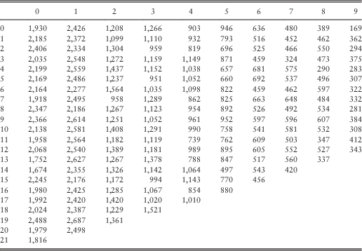
In Table 3 the CDR’s are given with the splits in the terms “change future”, “difference between forecast and observations”, “difference between updated forecast and observations” and “change in update”. Moreover, we give the conditional expected value of the CDR, which is always negative in this example. In the CDR we observe negative values in 5 consecutive years. More precisely, we have 10 times a loss in the 12 years from calendar years 10–21. This is also illustrated in the plots in Figure 1 and Figure 2. From the table and from the figures one can see that in this specific example the deviation of the forecasts from the observations in the newest diagonal contributes much more to the observed CDR than the effect of the parameter update for future years.
Claims development result (CDR) and split in “difference between updated forecast and observations” plus “change in update” and  $$E[{\rm CDR}_{t} {\rm \,\mid\,}{\cal I}_{{s_{0} }} ,{\cal D}_{{s_{0} {\minus}1}} ,\Psi _{{s_{0} }} ]$$
.
Claims development result (CDR) and split in “difference between forecast and observations” plus “change future”.
CDR, change future (Future), difference between forecast and observations (Forecast), difference between updated forecast and observations (Up forecast), change in update (Update), conditional expected value of the CDR and predictions  $$\Psi _{{s_{0} }}^{{(t)}} $$
.
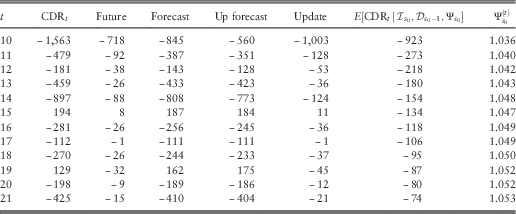
The predictions  $$\Psi _{{s_{0} }}^{{(t)}} $$
are given in Table 3 and a corresponding plot is given in Figure 3.
Predictions  $$\Psi _{{s_{0} }}^{{(t)}} $$
of
 $$\Psi _{{s_{0} }} $$
.
For illustrative purposes we have only considered one realisation of a claims triangle with the given diagonal effect  $$\psi _{{s_{0} }} $$
in the above example. We additionally simulate 10,000 triangles with this diagonal effect and consider the conditional distribution of the CDR. It is important to keep the diagonal effect fixed, because in the situation considered we have exactly one effect and therefore we should not average over different effects.
We give boxplots of the realised values of the CDR in the simulations in Figure 4. The conditional expected value is negative and we observe that it gets closer to zero in later calendar years. In the first few calendar years after the jump, it is likely to observe negative CDR’s.
Boxplot of CDRt, with 10,000 simulations,  $$\psi _{{s_{0} }} =1.05$$
.
In practice, there are usually several consecutive jumps, often going into the same direction over a period of years. Such situations reinforce the fact of having the same sign of the CDR over several consecutive years. In the next section we give a more general framework in order to model such cases more adequately.
3.3. Normal–Normal Model
In the real world, the process with regard to change of legislation is longer and not as simple as in the One Jump Model 3.2. For instance, there can be a first pending process on a lower court, then a first verdict followed by other processes and other verdicts possibly on the next higher courts, and sometimes the legal question is even brought to the highest Swiss Federal court whose verdicts have a precedent-setting character. All this can take several years. In the mathematical set-up this means that one has several consecutive jumps going in the same direction and thus reinforcing the fact of having the same sign of the CDR over several consecutive years.
Moreover, in the real world there can be several sources and events (change of legislation, economic factors and so on) that lead to a diagonal effect. Some of them lead to an additive change (jump) in the diagonal effects, others to a multiplicative one or to a combination of both. For instance, the impact of economic factors such as consumer price inflation on Ψt could possibly be modelled by an autoregressive process meaning that
 $$\Psi _{t} =\rho \Psi _{{t{\minus}1}} {\plus}(1{\minus}\rho ){\plus}\Delta _{t}, $$
where the Δt are i.i.d. with E[Δt]=0 (see also Shi et al., Reference Shi, Basu and Meyers2012).
The following model is quite general and allows to mathematically describe situations, where the diagonal effect Ψt can change dynamically in every calendar year in an additive or multiplicative manner or both. By dynamically we mean that the parameters  $$a_{{t{\plus}l}}^{{(t)}} $$
(multiplicative) and
 $$b_{{t{\plus}l}}^{{(t)}} $$
(additive) in Model Assumptions 3.5 depend on the information at time t and are therefore adjusted over time.
Model Assumptions 3.5 (Normal–Normal Model)
i) Conditionally, given Ψand  $${\cal I}_{t} ,$$
the X i,jare independent and normally distributed with
 $$\eqalignno{ & E\left[ {\left. {X_{{i,j}} } \right|{\bPsi},{\cal I}_{t} } \right]=E\left[ {\left. {X_{{i,j}} } \right|\Psi _{{i{\plus}j}} } \right]=\mu _{i} \gamma _{j} \Psi _{{i{\plus}j}}, \cr & {\rm Var}\left( {\left. {X_{{i,j}} } \right|{\bPsi},{\cal I}_{t} } \right)=\mu _{i} \eta _{j}^{2} \sigma ^{2}, $$
where  $$\mathop{\sum}\nolimits_{j=0}^J \gamma _{j} =\mathop{\sum}\nolimits_{j=0}^J \eta _{j}^{2} =1$$
.
ii) Conditionally, given  $${\cal I}_{t} $$
and
 $${\cal D}_{{t{\minus}1}} $$
, Ψtis normally distributed with
 $$\eqalignno{ \Psi _{t}^{{(t,t{\minus}1)}} := & E[\Psi _{t} {\rm \,\mid\,}{\cal I}_{t} ,{\cal D}_{{t{\minus}1}} ]=a_{t}^{{(t)}} \Psi _{{t{\minus}1}}^{{(t{\minus}1)}} {\plus}b_{t}^{{(t)}}, \cr q_{t}^{{(t,t{\minus}1)}} := & {\rm Var}(\Psi _{t} {\rm \,\mid\,}{\cal I}_{t} ,{\cal D}_{{t{\minus}1}} )=\left( {a_{t}^{{(t)}} } \right)^{2} q_{{t{\minus}1}}^{{(t{\minus}1)}} {\plus}\delta _{t}^{{2^{{(t)}} }}, $$
for t≥0 and  $$\Psi _{{{\minus}1}}^{{({\minus}1)}} =1$$
and
 $$q_{{{\minus}1}}^{{({\minus}1)}} =\tau ^{2} $$
.
iii) Conditionally, given  $${\cal I}_{t} $$
and
 $${\cal D}_{t} $$
,
 $$\Psi _{{t{\plus}l}}^{{(t)}} :=E[\Psi _{{t{\plus}l}} {\rm \,\mid\,}{\cal I}_{t} ,{\cal D}_{t} ]=a_{{t{\plus}l}}^{{(t)}} \Psi _{{t{\plus}l{\minus}1}}^{{(t)}} {\plus}b_{{t{\plus}l}}^{{(t)}} ,\quad l\geq 1,$$
and  $$a_{{t{\plus}l}}^{{(t)}} \geq 0$$
and
 $$b_{{t{\plus}l}}^{{(t)}} $$
are
 $$\sigma ({\cal I}_{t} ,{\cal D}_{{t{\minus}1}} )$$
measurable for l≥0.
iv) For 0≤l≤t,  $$\Psi _{{t{\minus}l}} {\rm \,\mid\,}({\cal I}_{t} ,{\cal D}_{{t{\minus}l}} )$$
has the same distribution as
 $$\Psi _{{t{\minus}l}} {\rm \,\mid\,}({\cal I}_{{t{\minus}l}} ,{\cal D}_{{t{\minus}l}} )$$
.
Remarks.
∙ The
$$a_{{t{\plus}l}}^{{(t)}} $$
,
$$b_{{t{\plus}l}}^{{(t)}} $$
and
$$\delta _{{t{\plus}l}}^{{2^{{(t)}} }} $$
steering the change from Ψt to Ψt+l also depend on
$${\cal I}_{t} $$
. Consider, for instance, the situation where there is a change of legislation in some year t and one expects that the incremental claim payments X i,j in future calendar years i+j>t will increase by some percentage, but one is uncertain about the exact value of this percentage. Such situations can be taken into account by a suitable choice of
$$b_{{t{\plus}l}}^{{(t)}} $$
and
$$\delta _{{t{\plus}l}}^{{2^{{(t)}} }} $$
.∙ Note that by assumption iii), at time t we include the possibility of expected jumps and/or trends in the future.
∙ In the incurred triangle, there are several possible situations such as the introduction of new guidelines in the claims department, staff fluctuation, changes in legislation, which can lead to higher uncertainties in the case estimates. Such situations can be taken into account by replacing the variance assumption (12) in the model by


 $${\rm Var}\left( {\left. {X_{{i,j}} } \right|{\bPsi},{\cal I}_{t} } \right)=\mu _{i} \eta _{j}^{2} \sigma ^{2} c_{{i{\plus}j}}^{{2^{{(t)}} }} ,$$
where  $$c_{{i{\plus}j}}^{{2^{{(t)}} }} $$
are constants depending on the external information
 $${\cal I}_{t} $$
and
 $$c_{{i{\plus}j}}^{{2^{{(t)}} }} =c_{{i{\plus}j}}^{{2^{{(i{\plus}j)}} }} $$
for
 $$i{\plus}j\leq t$$
.
∙ Special cases:
− If we assume that the diagonal effects are given by
with independent
$$\Psi _{t} =1{\plus}\Delta _{t} ,\quad E[\Delta _{t} {\rm \,\mid\,}{\cal I}_{t} ]=0,$$
$$\Delta _{t} $$
then the diagonal effects of different calendar years are independent. This can be modelled by choosing
$$a_{{t{\plus}l}}^{{(t)}} \,\equiv\,0$$
and
$$b_{{t{\plus}l}}^{{(t)}} \,\equiv\,1$$
for
$$l\geq 0$$
and all
$$t$$
.− The stationary AR
$$(1)$$
processcan be modelled by choosing
$$\Psi _{{t{\plus}l}} =\rho \Psi _{{t{\plus}l{\minus}1}} {\plus}(1{\minus}\rho ){\plus}\Delta _{{t{\plus}l}}, $$
$$a_{{t{\plus}l}}^{{(t)}} \,\equiv\,\rho $$
,
$$b_{{t{\plus}l}}^{{(t)}} \,\equiv\,(1{\minus}\rho )$$
and
$$\tau ^{2} =\delta ^{2} /(1{\minus}\rho ^{2} )$$
. The formula for
$$\Psi _{t}^{{(t,t{\minus}1)}} $$
is then a weighted average between the last prediction and the initial estimate
$$1$$
:Similarly for the quadratic loss
$$\Psi _{t}^{{(t,t{\minus}1)}} =\rho \Psi _{{t{\minus}1}}^{{(t{\minus}1)}} {\plus}(1{\minus}\rho ).$$
$$q^{{(t,t{\minus}1)}} $$
we have the weighted average
$$q^{{(t,t{\minus}1)}} =\rho ^{2} q_{{t{\minus}1}}^{{(t{\minus}1)}} {\plus}(1{\minus}\rho ^{2} )\tau ^{2}. $$
∙ In practice one also needs to estimate the parameters
$$\gamma _{j} $$
and
$$\mu _{i} $$
. But as already mentioned in section 1.2 this is not an essential point for the message of this paper and we therefore assume that they are known.


In the following theorem we show that under Model Assumptions 3.5 there exists a recursive procedure to calculate the predictors  $$\Psi _{t}^{{\left( t \right)}} $$
and the corresponding conditional msep’s:
 $$q_{t}^{{(t)}} ={\rm Var}(\Psi _{t} \,\mid\,{\cal I}_{t} ,{\cal D}_{t} )=E\left[ {\left. {\left( {\Psi _{t} {\minus}\Psi _{t}^{{(t)}} } \right)^{2} } \right|{\cal I}_{t} } \right].$$
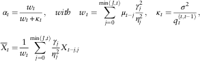
Theorem 3.6 (recursive procedure, Normal–Normal Model) Under Model Assumptions 3.5  $$\Psi _{{t{\plus}k}}^{{(t)}} $$
and
 $$q_{t}^{{(t)}} $$
can be calculated by the following recursive procedure:
i) Initialisation:
$$\Psi _{{{\minus}1}}^{{({\minus}1)}} =1,\quad q_{{{\minus}1}}^{{({\minus}1)}} =\tau ^{2}. $$
ii) For
$$t\geq 0$$
:a) Update in the newest diagonal:
where
$$\Psi _{t}^{{(t)}} =\alpha _{t} \bar{X}_{t} {\plus}\left( {1{\minus}\alpha _{t} } \right)\Psi _{t}^{{(t,t{\minus}1)}}, $$
and
$$\eqalignno{ \alpha _{t} = & {{w_{t} } \over {w_{t} {\plus}\kappa _{t} }},\quad with\quad w_{t} =\mathop{\sum}\limits_{j=0}^{{\rm min}(\,J,t)\wedget} \mu _{{t{\minus}j}} {{\gamma _{j}^{2} } \over {\eta _{j}^{2} }},\quad \kappa _{t} ={{\sigma ^{2} } \over {q_{t}^{{(t,t{\minus}1)}} }}, \cr \bar{X}_{t} = & {1 \over {w_{t} }}\mathop{\sum}\limits_{j=0}^{{\rm min}(\,J,t)\wedget} {{\gamma _{j} } \over {\eta _{j}^{2} }}X_{{t{\minus}j,j}} $$
$$q_{t}^{{(t)}} =(1{\minus}\alpha _{t} )q_{t}^{{(t,t{\minus}1)}}. $$
b) Forecast of future diagonal effects: for k≥1:
$$\Psi _{{t{\plus}k}}^{{(t)}} =a_{{t{\plus}k}}^{{(t)}} \Psi _{{t{\plus}k{\minus}1}}^{{(t)}} {\plus}b_{{t{\plus}k}}^{{(t)}}. $$




Remarks.
∙ If we drop the normal assumptions and do not make any distributional assumptions, Theroem 3.6 still yields the credibility estimators.
∙ Special cases:
- For independent diagonal effects Ψt=1+Δt, with
$$\Delta _{t} {\rm \,\mid\,}{\cal I}_{t} \,\sim\,N(0,\delta _{t}^{{2^{{(t)}} }} )$$
, we get the predictorsAs in this case the diagonal effects of different calendar years are independent,
$$\Psi _{t}^{{(t)}} =\alpha _{t} \bar{X}_{t} {\plus}(1{\minus}\alpha _{t} ),\quad {\rm where}\quad \alpha _{t} ={{w_{t} } \over {w_{t} {\plus}{{\sigma ^{2} } \over {\delta _{t}^{{2^{{(t)}} }} }}}}.$$
$$\Psi _{t}^{{(t)}} $$
depends only on the observations of calendar year t.- In case of the AR(1) process (14) we obtain
$$\eqalignno{ \Psi _{t}^{{(t)}} = & \alpha _{t} \bar{X}_{t} {\plus}(1{\minus}\alpha _{t} )\left( {\rho \Psi _{{t{\minus}1}}^{{(t{\minus}1)}} {\plus}(1{\minus}\rho )} \right), \cr q_{t}^{{(t)}} = & (1{\minus}\alpha _{t} )\left( {\rho ^{2} q_{{t{\minus}1}}^{{(t{\minus}1)}} {\plus}(1{\minus}\rho ^{2} )\tau ^{2} } \right). $$


Proof of Theorem 3.6: The formulas for  $$\Psi _{t}^{{(t)}} $$
and
 $$q_{t}^{{(t)}} $$
follow from the posterior distribution of Ψt, given
 $${\cal I}_{t} $$
and
 $${\cal D}_{t} $$
:
 $$\eqalignno{ f_{{\Psi _{t} \,\mid\,{\cal I}_{t} ,{\cal D}_{t} }} & \propto\exp \left( {{\minus}{{\left( {\Psi _{t} {\minus}\Psi _{t}^{{(t,t{\minus}1)}} } \right)^{2} } \over {2q_{t}^{{(t,t{\minus}1)}} }}} \right)\prod\limits_{i{\plus}j=t} \exp \left( {{\minus}{{\left( {X_{{i,j}} {\minus}\mu _{i} \gamma _{j} \Psi _{t} } \right)^{2} } \over {2\mu _{i} \eta _{j}^{2} \sigma ^{2} }}} \right) \cr \propto\exp \left( {{\minus}{1 \over 2}\left( {\Psi _{t}^{2} \left( {\mathop{\sum}\limits_{i{\plus}j=t} {{\mu _{i} \gamma _{j}^{2} } \over {\eta _{j}^{2} \sigma ^{2} }}{\plus}{1 \over {q_{t}^{{(t,t{\minus}1)}} }}} \right){\minus}2\Psi _{t} \left( {\mathop{\sum}\limits_{i{\plus}j=t} {{\gamma _{j} X_{{i,j}} } \over {\eta _{j}^{2} \sigma ^{2} }}{\plus}{{\Psi _{t}^{{(t,t{\minus}1)}} } \over {q_{t}^{{(t,t{\minus}1)}} }}} \right)} \right)} \right). $$
Hence we obtain
 $$\Psi _{t}^{{(t)}} =E\left[ {\left. {\Psi _{t} } \right|{\cal I}_{t} ,{\cal D}_{t} } \right]={{\mathop{\sum}\limits_{i{\plus}j=t} {{\gamma _{j} X_{{i,j}} } \over {\eta _{j}^{2} \sigma ^{2} }}{\plus}{{\Psi _{t}^{{(t,t{\minus}1)}} } \over {q_{t}^{{(t,t{\minus}1)}} }}} \over {\mathop{\sum}\limits_{i{\plus}j=t} {{\mu _{i} \gamma _{j}^{2} } \over {\eta _{j}^{2} \sigma ^{2} }}{\plus}{1 \over {q_{t}^{{(t,t{\minus}1)}} }}}}=\alpha _{t} \bar{X}_{t} {\plus}(1{\minus}\alpha _{t} )\Psi _{t}^{{(t,t{\minus}1)}} $$
and
 $$q_{t}^{{(t)}} ={\rm Var}(\Psi _{t} {\rm \,\mid\,}{\cal I}_{t} ,{\cal D}_{t} )={1 \over {\mathop{\sum}\limits_{i{\plus}j=t} {{\mu _{i} \gamma _{j}^{2} } \over {\eta _{j}^{2} \sigma ^{2} }}{\plus}{1 \over {q_{t}^{{(t,t{\minus}1)}} }}}}=(1{\minus}\alpha _{t} )q_{t}^{{(t,t{\minus}1)}}. $$
As in section 3.2 one can derive a formula for the conditional expected value of the CDR. For the CDR we obtain under Model Assumptions 3.5 from equation (8)
 $${\rm CDR}_{{t{\plus}1}} =\Psi _{{t{\plus}1}}^{{(t{\plus}1)}} \mathop{\sum}\limits_{j=1}^J \mu _{{t{\plus}1{\minus}j}} \gamma _{j} {\minus}\mathop{\sum}\limits_{j=1}^J X_{{t{\plus}1{\minus}j,j}} {\plus}\mathop{\sum}\limits_{k=1}^J \left( {\Psi _{{t{\plus}k}}^{{(t)}} {\minus}\Psi _{{t{\plus}k}}^{{(t{\plus}1)}} } \right)\mathop{\sum}\limits_{j=k}^J \mu _{{t{\plus}k{\minus}j}} \gamma _{j}. $$
In the appendix we derive the following formula for the conditional expected value of the CDR
 $$\eqalignno{ E\left[ {\left. {CDR_{{t{\plus}1}} } \right|{\cal I}_{{t{\plus}1}} ,{\cal D}_{t} ,\Psi } \right] \cr & =\left( {\Psi _{{t{\plus}1}}^{{(t{\plus}1,t)}} {\minus}\Psi _{{t{\plus}1}} } \right)\left( {\mathop{\sum}\limits_{j=1}^J \mu _{{t{\plus}1{\minus}j}} \gamma _{j} {\plus}\alpha _{{t{\plus}1}} \mathop{\sum}\limits_{k=2}^J \prod\limits_{l=2}^k a_{{t{\plus}l}}^{{(t{\plus}1)}} \mathop{\sum}\limits_{j=k}^J \mu _{{t{\plus}k{\minus}j}} \gamma _{j} } \right) \cr & \quad {\plus}\mathop{\sum}\limits_{k=1}^J \left( {\Psi _{t}^{{(t)}} \left( {\prod\limits_{l=1}^k a_{{t{\plus}l}}^{{(t)}} {\minus}\prod\limits_{l=1}^k a_{{t{\plus}l}}^{{(t{\plus}1)}} } \right){\plus}\mathop{\sum}\limits_{l=1}^k \left( {b_{{t{\plus}l}}^{{(t)}} \prod\limits_{n=l{\plus}1}^k a_{{t{\plus}n}}^{{(t)}} {\minus}b_{{t{\plus}l}}^{{(t{\plus}1)}} \prod\limits_{n=l{\plus}1}^k a_{{t{\plus}n}}^{{(t{\plus}1)}} } \right)} \right) \cr & \quad \quad {\times}\mathop{\sum}\limits_{j=k}^J \mu _{{t{\plus}k{\minus}j}} \gamma _{j}, $$
where Ψ={Ψ0,Ψ1, …}. The cases of interest are the situations where the diagonal effects change in the same direction (increase or decrease) over several years. It is likely that in such situations the effects are underestimated (as in the example of motor liability in Switzerland) and in such a case the conditional expected value of the CDR has the same sign over several consecutive years. More details on this are given in the appendix.
4. Concluding remarks
The primary aim of this paper was to show that the same sign of the CDR over several consecutive calendar years is not a contradiction to best estimate reserves. This has already been achieved by considering the One Jump Model 3.2.
More realistic situations can be mathematically well described by the Normal–Normal Model 3.5 introduced in section 3.3. This model is quite general and covers a variety of real-life situations.
Impacts of changes in the claims’ environment are usually first detected in the incurred claims figures, whereas they often only appear in the paid triangle with a time lag. The reason is that the claims’ adjusters can react much quicker to such changes by adjusting their case estimates accordingly, which is then seen as a diagonal effect in the incurred triangle. For this reason reserving actuaries are usually looking at both, the paid and the incurred triangle. It might happen that the claims adjusters overreact in their case estimates. However, it will not be possible to see, whether and to which extent an observed trend in the newest diagonal of the incurred triangle is systematic or due to “overreaction”. But the actuary will know that there is a higher uncertainty in the incurred claims figures, which can be taken into account by the time-dependent parameters  $$c_{{i{\plus}j}}^{{2(t)}} $$
as given in equation (13). For the best estimate reserves it turns out from Theorem 3.6 by replacing σ 2 by σ 2c t2(t), that the higher the uncertainty, the less weight is given to the observations in the newest diagonal. This result reflects what we expect and what is also done in practice, although more by intuition than in a systematic way.
In our model we have assumed that there is the same diagonal factor for all elements of a diagonal. There can be situations, where this not the case, for instance, if a change of legislation only has an impact on bodily injury claims. Our modelling framework can be extended to such situations by assuming that the diagonal effects are random vectors rather than random variables. But this is beyond the aim and the scope of this paper.
In this paper we have considered full Bayesian models in order to be able to explicitly calculate best estimate reserves defined as the posterior expected values of future claim payments. One might object that a normal distribution is not a realistic assumption for claims data but one can easily drop the distributional assumptions and switch to a corresponding credibility model and credibility estimators. But this is again out of the primary goal and scope of this paper. The same holds for μ i and γ j, which were assumed to be known. Of course, in practice one will have to estimate them.
We want to emphasise once more that in our model the expert opinion changes over time. This idea can also be found in De Jong & Zehnwirth (Reference De Jong and Zehnwirth1983). However, in most of the actuarial literature on Bayes- and credibility models there is only one a priori distribution not changing over time. We believe that models that allow for changing expert opinions over time have a big potential to bring models nearer to the processes in the real world and to solve problems in practice, not only for reserving but also for pricing and other applications.
Acknowledgements
The authors would like to thank two anonymous referees for valuable comments that helped to improve an earlier version of this paper.
Appendix
As in the case of the One Jump Model 3.2, we want to study the signs of consecutive CDR’s in the Normal-Normal Model 3.5. For this purpose we consider a conditional expected value of the CDR. Recall the CDR under Model Assumptions 3.5:
 $${\rm CDR}_{{t{\plus}1}} =\Psi _{{t{\plus}1}}^{{(t{\plus}1)}} \mathop{\sum}\limits_{j=1}^J \mu _{{t{\plus}1{\minus}j}} \gamma _{j} {\minus}\mathop{\sum}\limits_{j=1}^J X_{{t{\plus}1{\minus}j,j}} {\plus}\mathop{\sum}\limits_{k=1}^J \left( {\Psi _{{t{\plus}k}}^{{(t)}} {\minus}\Psi _{{t{\plus}k}}^{{(t{\plus}1)}} } \right)\mathop{\sum}\limits_{j=k}^J \mu _{{t{\plus}k{\minus}j}} \gamma _{j} $$
and conditionally on Ψ={Ψ0,Ψ1, …} we get
 $$\eqalignno{ E\left[ {\left. {{\rm CDR}_{{t{\plus}1}} } \right|{\cal I}_{{t{\plus}1}} ,{\cal D}_{t} ,\Psi } \right]= & (1{\minus}\alpha _{{t{\plus}1}} )\left( {\Psi _{{t{\plus}1}}^{{(t{\plus}1,t)}} {\minus}\Psi _{{t{\plus}1}} } \right)\mathop{\sum}\limits_{j=1}^J \mu _{{t{\plus}1{\minus}j}} \gamma _{j} \cr & \quad {\plus}\mathop{\sum}\limits_{k=1}^J \left( {\Psi _{{t{\plus}k}}^{{(t)}} {\minus}E\left[ {\left. {\Psi _{{t{\plus}k}}^{{(t{\plus}1)}} } \right|{\cal I}_{{t{\plus}1}} ,{\cal D}_{t} ,Y} \right]} \right)\mathop{\sum}\limits_{j=k}^J \mu _{{t{\plus}k{\minus}j}} \gamma _{j}. $$
Note that for k≥1
 $$\eqalignno{ \Psi _{{t{\plus}k}}^{{(t)}} = & \Psi _{t}^{{(t)}} \prod\limits_{l=t{\plus}1}^{t{\plus}k} a_{l}^{{(t)}} {\plus}\mathop{\sum}\limits_{l=t{\plus}1}^{t{\plus}k} b_{l}^{{(t)}} \prod\limits_{n=l{\plus}1}^{t{\plus}k} a_{n}^{{(t)}}, \cr \Psi _{{t{\plus}k}}^{{(t{\plus}1)}} = & \Psi _{{t{\plus}1}}^{{(t{\plus}1)}} \prod\limits_{l=t{\plus}2}^{t{\plus}k} a_{l}^{{(t{\plus}1)}} {\plus}\mathop{\sum}\limits_{l=t{\plus}2}^{t{\plus}k} b_{l}^{{(t{\plus}1)}} \prod\limits_{n=l{\plus}1}^{t{\plus}k} a_{n}^{{(t{\plus}1)}}, $$
and hence
 $$\eqalignno{ \Psi _{{t{\plus}k}}^{{(t)}} & {\minus}E\left[ {\left. {\Psi _{{t{\plus}k}}^{{(t{\plus}1)}} } \right|{\cal I}_{{t{\plus}1}} ,{\cal D}_{t} ,\Psi } \right] \cr = & \Psi _{t}^{{(t)}} \left( {\prod\limits_{l=t{\plus}1}^{t{\plus}k} a_{l}^{{(t)}} {\minus}\prod\limits_{l=t{\plus}1}^{t{\plus}k} a_{l}^{{(t{\plus}1)}} } \right){\plus}\mathop{\sum}\limits_{l=t{\plus}1}^{t{\plus}k} \left( {b_{l}^{{(t)}} \prod\limits_{n=l{\plus}1}^{t{\plus}k} a_{n}^{{(t)}} {\minus}b_{l}^{{(t{\plus}1)}} \prod\limits_{n=l{\plus}1}^{t{\plus}k} a_{n}^{{(t{\plus}1)}} } \right) \cr & \quad {\plus}\alpha _{{t{\plus}1}} \left( {\Psi _{{t{\plus}1}}^{{(t{\plus}1,t)}} {\minus}\Psi _{{t{\plus}1}} } \right)\prod\limits_{l=t{\plus}2}^{t{\plus}k} a_{l}^{{(t{\plus}1)}}. $$
It follows that
 $$\eqalignno{ E\left[ {\left. {CDR_{{t{\plus}1}} } \right|{\cal I}_{{t{\plus}1}} ,{\cal D}_{t} ,\Psi } \right] &=\left( {\Psi _{{t{\plus}1}}^{{(t{\plus}1,t)}} {\minus}\Psi _{{t{\plus}1}} } \right)\left( {\mathop{\sum}\limits_{j=1}^J \mu _{{t{\plus}1{\minus}j}} \gamma _{j} {\plus}\alpha _{{t{\plus}1}} \mathop{\sum}\limits_{k=2}^J \prod\limits_{l=2}^k a_{{t{\plus}l}}^{{(t{\plus}1)}} \mathop{\sum}\limits_{j=k}^J \mu _{{t{\plus}k{\minus}j}} \gamma _{j} } \right) \cr & \quad & {\plus}\mathop{\sum}\limits_{k=1}^J \left( {\Psi _{t}^{{(t)}} \left( {\prod\limits_{l=1}^k a_{{t{\plus}l}}^{{(t)}} {\minus}\prod\limits_{l=1}^k a_{{t{\plus}l}}^{{(t{\plus}1)}} } \right){\plus}\mathop{\sum}\limits_{l=1}^k \left( {b_{{t{\plus}l}}^{{(t)}} \prod\limits_{n=l{\plus}1}^k a_{{t{\plus}n}}^{{(t)}} {\minus}b_{{t{\plus}l}}^{{(t{\plus}1)}} \prod\limits_{n=l{\plus}1}^k a_{{t{\plus}n}}^{{(t{\plus}1)}} } \right)} \right) \cr &\quad{\times}\mathop{\sum}\limits_{j=k}^J \mu _{{t{\plus}k{\minus}j}} \gamma _{j}. $$
In order to analyse this term, we assume that γ j≥0 for all j.
Let us consider the situation where a new phenomenon leads to an increase in the diagonal effects that is,  $$\Psi _{t} \leq \Psi _{{t{\plus}1}} \leq \,\ldots\,\leq \Psi _{{t{\plus}n}} $$
for some n>1. It is likely that this increase is at first underestimated (as in the example of motor liability in Switzerland) and hence it is plausible that for l≥1 and for some k≥1:
 $$\eqalignno{ & a_{{t{\plus}l}}^{{(t)}} \leq a_{{t{\plus}l}}^{{(t{\plus}1)}} \leq a_{{t{\plus}l}}^{{(t{\plus}2)}} \leq \,\ldots\,\leq a_{{t{\plus}l}}^{{(t{\plus}k)}}, \cr & b_{{t{\plus}l}}^{{(t)}} \leq b_{{t{\plus}l}}^{{(t{\plus}1)}} \leq b_{{t{\plus}l}}^{{(t{\plus}2)}} \leq \,\ldots\,\leq b_{{t{\plus}l}}^{{(t{\plus}k)}}, $$
and  $$\Psi _{{t{\plus}1}}^{{(t{\plus}1,t)}} {\minus}\Psi _{{t{\plus}1}} \lt 0$$
for several consecutive calendar years t. This then leads to a negative sign of the conditionally expected CDR’s for several consecutive years. Analogously, this argument applies in the case of a decreasing effect which is first underestimated. Therefore, in the cases where the diagonal effects change in the same direction (increase or decrease) over several years, it is likely that this effect is underestimated and that one observes the same sign of the CDR over the corresponding years.