


1. Introduction
Heat and energy transported by convection regulate the climate and support life on Earth. Examples of planetary-scale convective processes include the circulation within the atmosphere, oceans (Vallis Reference Vallis2017; Forget & Ferreira Reference Forget and Ferreira2019), geothermal fluxes across the lithosphere (Grant & Bixley Reference Grant and Bixley2011; Letelier et al. Reference Letelier, O'Sullivan, Reich, Veloso, Sánchez-Alfaro, Aravena, Muñoz and Morata2021) and the mantle dynamics (Korenaga Reference Korenaga2020; Tackley Reference Tackley2000).
The fundamentals of heat and energy transport in free three-dimensional flows (Ahlers, Funfschilling & Bodenschatz Reference Ahlers, Funfschilling and Bodenschatz2009a; Grossmann & Lohse Reference Grossmann and Lohse2011; Hughes, Gayen & Griffiths Reference Hughes, Gayen and Griffiths2013) and porous media (Doering & Constantin Reference Doering and Constantin1998; Hewitt, Neufeld & Lister Reference Hewitt, Neufeld and Lister2012; Nield & Bejan Reference Nield and Bejan2013; Hewitt Reference Hewitt2020) have been extensively investigated via the classic Rayleigh–Bénard convection (RBC) problem. However, in highly confined environments where fluids are not entirely free to develop three-dimensional convection, heat transport and its link with energy fluxes remain uncharacterised. Such systems include geothermally driven flows across open fractures (Letelier et al. Reference Letelier, O'Sullivan, Reich, Veloso, Sánchez-Alfaro, Aravena, Muñoz and Morata2021) and near-surface flows in fractures observed in the ice shell of the solar system moons Enceladus and Europa (Le Gall et al. Reference Le Gall2017; Sparks et al. Reference Sparks, Schmidt, McGrath, Hand, Spencer, Cracraft and Deustua2017; Le Reun & Hewitt Reference Le Reun and Hewitt2020). In the above examples, convection can be examined at the laboratory scale using Hele-Shaw cells (Hidalgo et al. Reference Hidalgo, Fe, Cueto-Felgueroso and Juanes2012; Cooper et al. Reference Cooper, Crews, Schumer, Breitmeyer, Voepel and Decker2014; Letelier et al. Reference Letelier, Herrera, Mujica and Ortega2016). Studying the energy transfer rates, or energetics, of thermally driven flows in Hele-Shaw cells is therefore significant to unravelling energy pathways and their link with heat transport and mixing processes within fractured solid environments.
Winters et al. (Reference Winters, Lombard, Riley and D'Asaro1995) introduced a mathematical formalism to characterise the energetics and mixing of Boussinesq flows. Their formalism allows decomposition of the system's potential energy into a reference state of minimum or background potential energy (BPE) and the available potential energy (APE) to drive motion and enhance mixing. A strength of the APE–BPE framework is that it enables quantification of the irreversible diascalar mixing rate responsible for depleting the APE in a system. The latter is possible by knowing the density field  $\rho$ and the equilibrium position
 $z_{\star }$ of the fluid parcels that constitute the domain. Although determining the function
 $z_{\star }(\rho )$ – and its derivatives – from field observations may be challenging and involve approximations (e.g. Winters & D'Asaro Reference Winters and D'Asaro1996),
 $z_{\star }(\rho )$ can be computed robustly from high-fidelity numerical simulations in cylindrical and closed domains via standard sorting algorithms (Winters & Barkan Reference Winters and Barkan2013). Thus the APE–BPE framework represents a sound approach to characterise the energetics and mixing of RBC in Hele-Shaw cells (HS-RBC).
Recently, Caulfield (Reference Caulfield2021) emphasised that there is a close connection between the buoyancy variance and the APE of a system, especially in flows with a constant background buoyancy gradient. The latter is the case for the Earth's subsurface, which has a geothermal gradient of approximately  $30\,^{\circ }\textrm {C}\ \textrm {km}^{-1}$ (Dickson & Fanelli Reference Dickson and Fanelli2013). Yet many regions, such as hot spots in oceans, volcanic arcs along subduction zones and continental areas with a high density of fractures, have greater geothermal gradients. This geothermal gradient plays a critical role on the onset and development of convection in deep sedimentary aquifers and through fractured crystalline rocks (Murphy Reference Murphy1979; Tournier, Genthon & Rabinowicz Reference Tournier, Genthon and Rabinowicz2000). If the system's potential energy can be written in terms of the APE–BPE decomposition, the question here is whether a different decomposition could be directly expressed in terms of the temperature variance and hold the same information on the energy transfer rates.
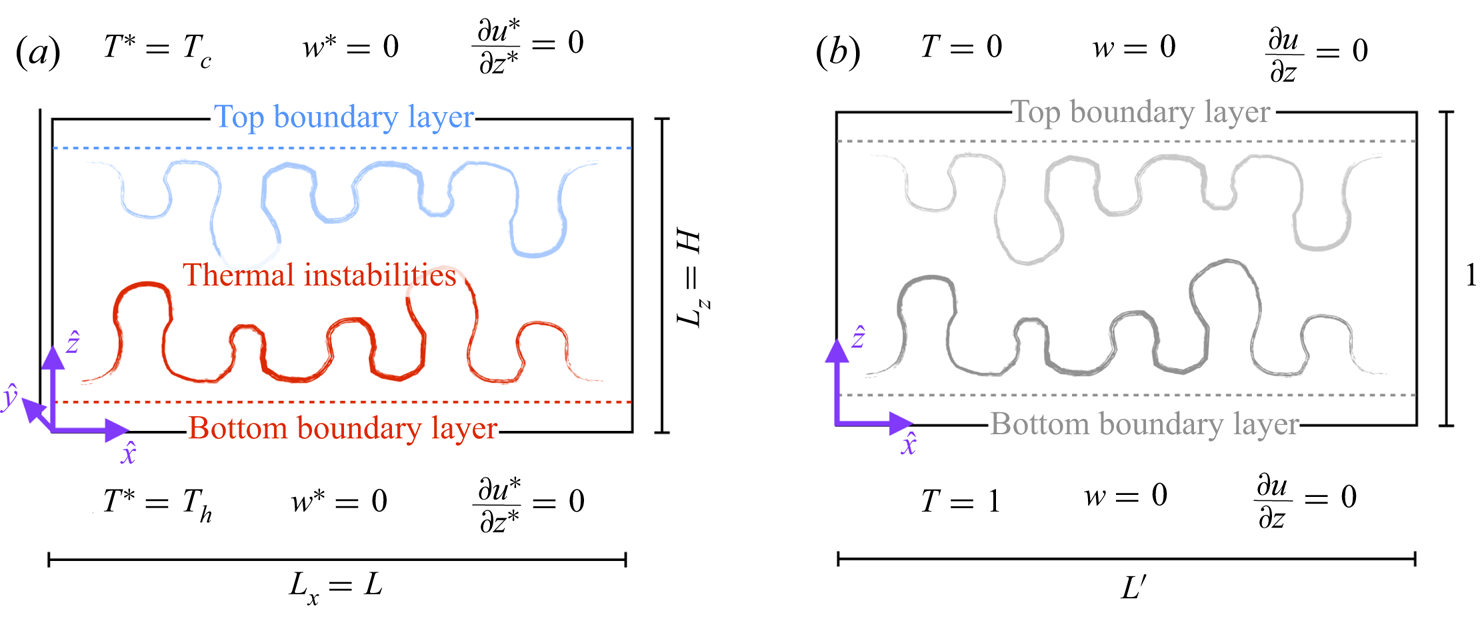
This paper focuses on investigating the energy pathways and their inherent link with heat transfer and mixing of HS-RBC (figure 1). For the above, it is essential to determine the energetics associated with surface thermal forcing, convective buoyancy transport and irreversible dissipative mechanisms – i.e. the rates of kinetic energy dissipation and thermal mixing.
Schematic of a Hele-Shaw cell adopted to investigate the fluid dynamics of geometrically constrained flows energised by constant temperature conditions at the bottom  $(T_h)$ and top
 $(T_c)$, with
 $T_{h}>T_{c}$. (a) Boundary conditions evaluated at
 $z^{*} = 0$ and
 $z^{*} = H$, while for
 $x^{*} = 0$ and
 $x^{*} = L$ we have periodic boundary conditions. (b) Non-dimensional representation of the boundary conditions of the problem. The two-dimensional Hele-Shaw model in (2.2), valid for the
 $XZ$ plane, is derived considering adiabatic and no-slip wall conditions at
 $y^{*}=0$ and
 $y^{*}=b$.

Building upon the Hele-Shaw equations derived in Letelier, Mujica & Ortega (Reference Letelier, Mujica and Ortega2019), which represent an extension of the Darcy model for permeable media, we introduce the mechanical energy budget and the efficiencies of HS-RBC. The energetics are derived following the APE–BPE framework (Winters et al. Reference Winters, Lombard, Riley and D'Asaro1995) and a different potential energy decomposition whose reference state is determined from the scalar fluctuations. Deriving the energetics and efficiencies for HS-RBC based on two different frameworks has an advantage. On the one hand, the APE–BPE decomposition is widely used for the study of turbulent mixing in stratified flows (e.g. Peltier & Caulfield Reference Peltier and Caulfield2003; Caulfield Reference Caulfield2020), and it provides a readable interpretation and comparison with other studies on convective flows (e.g. Hughes et al. Reference Hughes, Gayen and Griffiths2013; Davies Wykes, Hughes & Dalziel Reference Davies Wykes, Hughes and Dalziel2015; Winters et al. Reference Winters, Ulloa, Wüest and Bouffard2019). On the other hand, the new potential energy decomposition brings new insights into the system's energy partitioning and the energy flux supplied at the boundaries for the HS-RBC problem. Instead of using the BPE reference state, the new potential energy decomposition considers a reference potential energy linked to the quadratic scalar field potential, also known as the temperature variance (Zilitinkevich et al. Reference Zilitinkevich, Elperin, Kleeorin and Rogachevskii2007), a simple quantity to compute.
For HS-RBC, the two energetics frameworks here introduced are mathematically linked and lead to the same non-dimensional analytical expressions for the energy transfer rates and efficiencies. We show that the relationship between the energy partition and the heat transfer across the thermal boundary layers (TBLs) in permeable media is determined only by the Nusselt number  ${\textit {Nu}}$. Additionally, we illustrate the flow properties and the energetics of HS-RBC via a set of direct numerical simulations of the Hele-Shaw equations. The numerical experiments are discussed and compared with existing laboratory and numerical results (Otero et al. Reference Otero, Dontcheva, Johnston, Worthing, Kurganov, Petrova and Doering2004; Ahlers, Grossmann & Lohse Reference Ahlers, Grossmann and Lohse2009b; Hewitt et al. Reference Hewitt, Neufeld and Lister2012; Gayen, Hughes & Griffiths Reference Gayen, Hughes and Griffiths2013; Letelier et al. Reference Letelier, Mujica and Ortega2019), which allows us to provide a conceptual interpretation of the effects of geometrical control in three-dimensional RBC (3D-RBC). The mechanical energy framework and the numerical results here reported are relevant to the study and characterisation of thermally driven flows through natural fractures or artificial apertures in solids.
2. Hele-Shaw model
We consider an incompressible Boussinesq fluid in a three-dimensional Hele-Shaw domain whose cell gap is  $b$ in the
 $y^{*}$ direction, and whose horizontal length and vertical height are
 $L$ and
 $H$ in the
 $x^{*}$ and
 $z^{*}$ directions, respectively (figure 1). The permeability of the medium is
 $K = b^2/12$ and the kinematic viscosity
 $\nu _c$ and thermal diffusivity
 $\kappa _c$ are assumed to be constant and isotropic. The fluid density and temperature are considered to be linearly dependent as
 $\rho ^{*} = \rho _c - \alpha (T^{*}-T_c)$, with
 $\rho ^{*}(T_{c}) = \rho _{c}$ the reference value,
 $\alpha =\rho _{c}\tilde {\alpha }$ and
 $\tilde {\alpha }$ the thermal expansion coefficient. For convenience, we define the Boussinesq density component as
 $\tilde {\rho }^{*}=\rho ^{*}-\rho _{c}$. Here, we consider the following non-dimensional form of the dimensional variables
 $\{\boldsymbol {x}^{*},t^{*},\boldsymbol {v}^{*},p^{*},T^{*},\tilde {\rho }^{*}\}$,
 \begin{align} \boldsymbol{x} = \frac{\boldsymbol{x}^{*}}{H}, \quad t = \frac{t^{*}}{H/u_c'}, \quad \boldsymbol{v} = \frac{\boldsymbol{v}^{*}}{u_c'}, \quad p = \frac{\tilde{p}^{*}}{p_c},\! \quad\! T = \frac{(T^{*} - T_c)}{\Delta T}, \quad\!\textrm{and}\!\quad \rho = \frac{\tilde{\rho}^{*}}{\alpha\Delta T} ={-}T, \end{align}
with  $\boldsymbol {x} = x\,\hat {\boldsymbol {x}} + z\,\hat {\boldsymbol {z}}$, the position,
 $\boldsymbol{v} = u \hat{\boldsymbol{x}} +w \hat{\boldsymbol{z}}$ the velocity field,
 $\Delta T = T_h - T_c$ (
 $T_h>T_c$) the temperature difference between the top (
 $T_c$) and the bottom (
 $T_h$) boundaries (Letelier et al. Reference Letelier, Mujica and Ortega2019), g the gravity acceleration,
 $u'_{c} = \alpha \Delta TgK/(\rho '_c\nu _{c})$ the characteristic velocity and
 $p_{c}=\rho '_c\nu _{c}u'_{c}H/K$ the characteristic pressure in terms of a modified reference density
 $\rho '_{c} = (6/5)\rho _{c}$.
For  $b \ll H$, the non-dimensional, two-dimensional (2-D) Hele-Shaw model (Letelier et al. Reference Letelier, Mujica and Ortega2019) governing the fluid motion is given by
 $$\begin{gather} \epsilon^{2}\frac{Ra'}{Pr}\left(\frac{\partial v_i}{\partial t} + \frac{9}{7}v_j\partial_j v_i\right) ={-}\partial_i p + T\delta_{iz} - \frac{5}{6}v_i + \epsilon^{2}\partial_j^2 v_i - \frac{2}{35}\epsilon^{2} Ra'(v_j\partial_j T)\delta_{iz} + O(\epsilon^4) , \end{gather}$$
 $$\begin{gather}\frac{\partial T}{\partial t} + v_i\partial_i T = \frac{1}{Ra'}\partial_i^2T + \frac{2}{35}\epsilon^{2} Ra'\partial_j\left((v_i\partial_i T)v_j\right) + O(\epsilon^4) , \end{gather}$$
where  $\epsilon = \sqrt {K}/H$ is the anisotropy ratio,
 $Ra' = u'_{c}H/\kappa _{c}$ is the modified Rayleigh number, with
 $Ra = (6/5)Ra' = (\alpha \Delta T g K H)/(\rho _{c}\kappa _{c}\nu _{c})$ the classic Rayleigh number for Hele-Shaw cells (Letelier et al. Reference Letelier, Mujica and Ortega2019), and
 $Pr = \nu _{c}/\kappa _{c}$ is the Prandtl number. In this model, the velocity field
 $\boldsymbol{v}$ (
 $v_{i}$ in tensorial form) is divergence free.
The Hele-Shaw equations (2.2) are valid for  $\epsilon$ small,
 $Pr\geqslant 1$ and
 $\epsilon ^{2}\,Ra'\ll 1$. For
 $\epsilon \rightarrow 0$, and considering a fixed
 $ {\textit {Ra}}'$, the model (2.2) reduces to the Darcy equations coupled with the advection–diffusion model (Hewitt et al. Reference Hewitt, Neufeld and Lister2012). Recent laboratory experiments demonstrated that the theoretical bound
 $\epsilon ^{2} {\textit {Ra}}\ll 1$ is valid for the Hele-Shaw model (2.2) (De Paoli, Alipour & Soldati Reference De Paoli, Alipour and Soldati2020). Thus the Hele-Shaw model represents a ‘mathematical bridge’ between the Darcy and Navier–Stokes models.
We examine the problem of HS-RBC considering a periodic domain in the horizontal which is stress free at the top and bottom boundaries. The bottom and top boundary conditions for the temperature field are  $T(z=0)=1$ and
 $T(z=1)=0$ (figure 1).
Henceforth, we express mean quantities through the horizontal and domain averages of a function  $f(t,\boldsymbol {x})$ as
 \begin{equation} \langle\, f\rangle_h(t,z) = \frac{1}{L'}\int_{0}^{L'} f(t,\boldsymbol{x})\,\textrm{d}\kern0.06em x \quad \textrm{and}\quad \langle\, f\rangle(t) = \int_{0}^{1}\langle\, f\rangle_h(t,z)\,\textrm{d}z, \end{equation}
respectively, with  $L' = L/H$ the cell aspect ratio. In this paper, Gauss's theorem is expressed as follows:
 \begin{equation} \int^{1}_{0}\int^{L'}_{0} \partial_{j} f \, \textrm{d}\kern0.06em x\,\textrm{d}z = \oint_{\ell} f n_{j} \,\textrm{d}\ell, \end{equation}
where  $n_{j}$ is the unit normal vector to the surface
 $\ell$. Additionally, we express the time average of a function
 $\langle\, f\rangle (t)$ over a window of size
 $\tau$ as
 \begin{equation} \langle\, f\rangle_{\tau} = \frac{1}{\tau}\int_{t}^{t+\tau}\langle\, f\rangle(t')\,\textrm{d}t'. \end{equation}
If a function  $\langle\, f\rangle (t)$ is in a statistically steady-state (SSS) condition for
 $t > \tau _{\textit {s}}$, it satisfies
 \begin{gather}
\left\langle \frac{{\rm d}\langle\, f\rangle}{{\rm d}t} \right\rangle_{\tau} = 0 \quad
\textrm{and} \quad \langle\, f\rangle_{\tau} = K : \text{const.}, \ \text{for $\tau > 0$}.
\end{gather}
In the following, all physical variables and equations presented in this work are valid up to  $O(\epsilon ^2)$, which is enough to include the cell gap effects on the thermal dynamics if
 $\epsilon ^2 {\textit {Ra}}' \ll 1$ is fulfilled. Within this framework, the energetics derived from the Hele-Shaw model (2.2) approximate the actual energetics for 3-D Boussinesq fluid flows.
3. Energetics up to  $O(\epsilon ^2)$

From the Hele-Shaw model (2.2) and the boundary conditions in figure 1, we derive the evolution equations for the mechanical energy, i.e. the kinetic and gravitational potential energy balances, for HS-RBC. In order to simplify the algebra, we examine the gravitational potential energy budget in terms of the Boussinesq density only, introduced previously in § 2. In what follows, variables are expressed in non-dimensional form. Nonetheless, for completeness, Appendix A introduces the dimensional mechanical energy components.
3.1. Kinetic energy balance
We define the specific kinetic energy as  $E_{\textit {k}} = v_i^2/2$ and the mean kinetic energy as
 $\langle E_{\textit {k}} \rangle$. Multiplying the momentum equation (2.2) by ‘
 $v_{i}$’ and averaging over the domain using (2.3a,b), the evolution equation for
 $\langle E_k \rangle$ results in
 $$\begin{gather} \epsilon^{2}\frac{Ra'}{Pr}\,\frac{\textrm{d}\langle E_{\textit{k}} \rangle}{\textrm{d} t} + F^{(\textit{surf})}_{\textit{k}} = \langle \varPhi^{(\epsilon)}_{\textit{prod}}\rangle-\langle \varPhi^{(\epsilon)}_{\textit{diss}}\rangle , \end{gather}$$
 $$\begin{gather}F^{(\textit{surf})}_{\textit{k}} = \oint_{\ell} \left(\frac{9}{7}\epsilon^2 Ra' \frac{v^2_i}{2}v_j + pv_j + \frac{2}{35}\epsilon^2 Ra' wT v_j - \epsilon^2v_i \tau_{ij}\right) n_{j}\, \textrm{d}\ell , \end{gather}$$
 $$\begin{gather}\varPhi_{\textit{prod}}^{(\epsilon)} = wT + \frac{2}{35}\epsilon^2{\textit{Ra}}'Tv_j\partial_j w , \end{gather}$$
 $$\begin{gather}\varPhi_{\textit{diss}}^{(\epsilon)} = \frac{5}{6}v^{2}_i + \epsilon^2\tau_{ij}\partial_j v_i . \end{gather}$$
The term  $\tau _{ij}$ denotes the stress tensor. Considering the boundary conditions of the problem (figure 1), the net kinetic energy flux at the domain boundaries is
 $F^{(\textit {surf})}_{\textit {k}} = 0$, and therefore
 \begin{equation} \epsilon^{2}\frac{Ra'}{Pr}\,\frac{\textrm{d}\langle E_{\textit{k}} \rangle}{\textrm{d} t} = \langle \varPhi^{(\epsilon)}_{\textit{prod}}\rangle-\langle \varPhi^{(\epsilon)}_{\textit{diss}}\rangle . \end{equation}
In (3.2),  $\langle \varPhi _{\textit {prod}}^{(\epsilon )} \rangle$ is the production rate of convective energy, i.e. the work done by buoyancy and Hele-Shaw dispersion to transport heat mechanically across the medium. On the other hand,
 $\langle \varPhi _{\textit {diss}}^{(\epsilon )} \rangle$ quantifies the decay rate of kinetic energy controlled by the Darcy and Stokes viscous dissipation. Note that, for
 $\epsilon = 0$, we recover a classical result for RBC in porous media, in which the rate of kinetic energy production due to the buoyancy flux
 $\langle wT\rangle$ balances the rate of dissipation owing to Darcy dispersion
 $(5/6)\langle v_i^2\rangle$ (Nield & Bejan Reference Nield and Bejan2013).
3.2. Gravitational potential energy balance
We define the specific potential energy as  $E_{\textit {p}} = z\rho$, and the mean potential energy as
 $\langle E_{\textit {p}} \rangle$. The rate of change in time of
 $\langle E_{\textit {p}} \rangle$ is determined by considering that
 $\rho =-T$ and the transport equation (2.2b),
 $$\begin{gather} \frac{\textrm{d} \langle E_{\textit{p}} \rangle }{\textrm{d} t} +F^{(\textit{surf})}_{\textit{p}} = \frac{1}{Ra'}\langle \partial_z T\rangle -\langle \varPhi_{\textit{prod}}^{(\epsilon)} \rangle, \end{gather}$$
 $$\begin{gather}F^{(\textit{surf})}_{\textit{p}} = \frac{1}{L'}\oint_{\ell}\frac{1}{Ra'}z\partial_j T n_{j}\,\textrm{d}\ell + \frac{1}{L'}\oint_{\ell}\left[zT - \frac{2}{35}\epsilon^2Ra'\left(z\partial_i(Tv_i) - w T \right) \right]v_j n_{j}\, \textrm{d}\ell. \end{gather}$$
Notice that  $\langle E_{\textit {p}} \rangle = -\langle zT \rangle < 0$. Applying the boundary conditions of the system (figure 1), only the first term on the right-hand side of (3.3b) survives, leading to
 \begin{equation} \frac{\textrm{d} \langle E_{\textit{p}}\rangle}{\textrm{d}t} ={-} \left.\frac{1}{{\textit{Ra}}'}\frac{\partial \langle T\rangle_{h}}{\partial z}\right|_{z=1} - \frac{1}{{\textit{Ra}}'} - \langle \varPhi^{(\epsilon)}_{\textit{prod}}\rangle , \end{equation}
where  $({1}/{L'})\oint _{\ell }\langle z\partial _{j} T\rangle = (\partial _{z}\langle T\rangle _{h} )|_{z=1}$ and
 $\langle \partial _{z}T\rangle = -1$. Therefore, defining the Nusselt number (e.g. Hewitt et al. Reference Hewitt, Neufeld and Lister2012; Letelier et al. Reference Letelier, Mujica and Ortega2019) as
 \begin{equation} {\textit{Nu}}(t) = \left.-\frac{\partial\langle T\rangle_h}{\partial z}\large\right|_{z=0} ={-} \left.\frac{\partial\langle T\rangle_h}{\partial z}\large\right|_{z=1}, \end{equation}
the evolution equation for the mean potential energy reduces to
 \begin{equation} \frac{\textrm{d} \langle E_{\textit{p}}\rangle}{\textrm{d}t} =\frac{{\textit{Nu}}-1}{{\textit{Ra}}'} - \langle \varPhi^{(\epsilon)}_{\textit{prod}}\rangle. \end{equation}
In SSS conditions,  $\langle \textrm {d} \langle E_{\textit {p}} \rangle /\textrm {d}t\rangle _{\tau } = 0$, the energy transport due to convection in the inner domain balances the surface buoyancy fluxes resulting from thermal conduction across the TBLs. This balance allows the expression of the Nusselt number as
 $\langle {\textit {Nu}}\rangle _{\tau } = 1 + {\textit {Ra}}'\langle \varPhi ^{(\epsilon )}_{\textit {prod}}\rangle _{\tau }$, a result previously obtained for permanent conditions in the mean temperature field
 $\langle T\rangle$ (Letelier et al. Reference Letelier, Mujica and Ortega2019). If the mechanical energy
 $\langle E_{\textit {m}}\rangle = \langle E_{\textit {k}}\rangle + \langle E_{\textit {p}}\rangle$ is conserved, we obtain
 $\langle \textrm {d} \langle E_{\textit {k}}\rangle /\textrm {d}t\rangle _{\tau } = 0$, and consequently
 $\langle \varPhi ^{(\epsilon )}_{\textit {prod}}\rangle _{\tau } = \langle \varPhi ^{(\epsilon )}_{\textit {diss}}\rangle _{\tau }$.
3.3. APE and BPE decomposition (APE–BPE)
To determine the potential energy gained by the system due to heat supplied at the boundaries, and that is free to enhance convection,  $E_{\textit {p}}$ is traditionally decomposed into the background
 $E_{\textit {bp}}$ and available
 $E_{\textit {ap}}$ components (Winters et al. Reference Winters, Lombard, Riley and D'Asaro1995; Hughes et al. Reference Hughes, Gayen and Griffiths2013). The specific background potential energy
 $E_{\textit {bp}} = z_{\star } \rho$ defines the minimum potential energy attainable by adiabatically rearranging the fluid parcels to their equilibrium positions given by the function
 $z_{\star } = z_{\star }(\rho )$ (Winters et al. Reference Winters, Lombard, Riley and D'Asaro1995). This energy cannot drive fluid motion. On the other hand, the specific APE, defined as
 $E_{\textit {ap}} = E_{\textit {p}} - E_{\textit {bp}}$, quantifies the energy that is free to generate fluid motion and enhance mixing. Their mean quantities
 $\langle E_{\textit {ap}}\rangle$ and
 $\langle E_{\textit {bp}}\rangle$ are determined by
 \begin{equation} \langle E_{\textit{ap}}\rangle = \frac{1}{L'}\int^{1}_{0}\int^{L'}_{0} (z - z_{{\star}})\rho\, \textrm{d}\kern0.06em x\,\textrm{d}z\quad\textrm{and} \quad \langle E_{\textit{bp}}\rangle = \frac{1}{L'}\int^{1}_{0}\int^{L'}_{0} z_{{\star}}\rho\, \textrm{d}\kern0.06em x\,\textrm{d}z , \end{equation}
respectively, and they represent approximations of the actual available and background potential energies for 3-D geometries (see Appendices D and E). In the fixed Hele-Shaw domain,  $\textrm {d}\langle E_{\textit {bp}}\rangle /\textrm {d}t$ (3.7a,b) leads to
 \begin{equation} \frac{\textrm{d}\langle E_{\textit{bp}}\rangle}{\textrm{d}t} = \frac{1}{L'}\int^{1}_{0}\int^{L'}_{0} \rho\frac{\partial z_{{\star}}}{\partial t}\, \textrm{d}\kern0.06em x\,\textrm{d}z + \frac{1}{L'}\int^{1}_{0}\int^{L'}_{0} z_{{\star}}\frac{\partial\rho}{\partial t}\, \textrm{d}\kern0.06em x\,\textrm{d}z. \end{equation}
The first term on the right-hand side of (3.8) integrates zero (Winters et al. Reference Winters, Lombard, Riley and D'Asaro1995). Since  $\rho = -T$, we plug the transport equation (2.2b) into (3.8), obtaining
 $$\begin{gather} \frac{\textrm{d}\langle E_{\textit{bp}}\rangle}{\textrm{d}t} + F^{(\textit{surf})}_{\textit{bp}} = \langle \varPhi^{(\epsilon)}_{\textit{mix}}\rangle , \end{gather}$$
 $$\begin{gather}F^{(\textit{surf})}_{\textit{bp}} = \frac{1}{L'}\, \oint_{\ell} \frac{1}{Ra'} z_{{\star}}\partial_i Tn_i\,\textrm{d}\ell + \frac{1}{L'}\, \oint_{\ell}\left[\psi + \frac{2}{35} \epsilon^2 Ra' z_{{\star}}\partial_j(Tv_j) \right]v_i n_i\,\textrm{d}\ell. \end{gather}$$
Notice that  $\langle E_{\textit {bp}} \rangle = -\langle z_{\star } T \rangle < 0$. The term
 $F^{(\textit {surf})}_{\textit {bp}}$ integrates the surface fluxes acting on the mean BPE, with
 $\psi = \int _{\rho (\varOmega )} z_{\star }(\hat {\rho }) \,\textrm {d}{\hat {\rho }}$ and
 $\varOmega$ the Hele-Shaw domain. Applying the boundary conditions (figure 1), only the first term on the right-hand side of (3.9b) remains, and it reduces to
 \begin{equation} F^{(\textit{surf})}_{\textit{bp}} ={-} \frac{1}{Ra'}\left.\frac{\partial \langle T\rangle_{h}}{\partial z}\right|_{z=0}, \end{equation}
with  $z_{\star }(z=0)=1$ and
 $z_{\star }(z=1)=0$ (Hughes et al. Reference Hughes, Gayen and Griffiths2013). Besides, the right-hand side term in (3.9a) is defined as
 \begin{equation} \langle \varPhi^{(\epsilon)}_{\textit{mix}}\rangle = \left\langle \frac{\textrm{d} z_{{\star}}}{\textrm{d} T}\,\varPhi^{(\epsilon)}_{\textit{scalar}}\right\rangle, \end{equation}
where
 \begin{equation} \varPhi_{\textit{scalar}}^{(\epsilon)} =\frac{1}{{\textit{Ra}}'}\,(\partial_i T)^2 + \frac{2}{35}\,\epsilon^2 {\textit{Ra}}'\left(\partial_i(v_iT)\right)^2 , \end{equation}
is the scalar dissipation rate (Letelier et al. Reference Letelier, Mujica and Ortega2019), a positive definite flux. Since by construction  $\textrm {d}z_{\star }/{\textrm {d}T}>0$, then
 $\langle \varPhi ^{(\epsilon )}_{\textit {mix}} \rangle$ is also a positive definite flux, and it characterises the rate at which thermal mixing increases
 $\langle E_{\textit {bp}} \rangle$. Thus, the evolution equation for the mean BPE can be written as
 \begin{equation} \frac{\textrm{d}\langle E_{\textit{bp}}\rangle}{\textrm{d}t} ={-} \frac{{\textit{Nu}}}{Ra'} + \langle \varPhi^{(\epsilon)}_{\textit{mix}}\rangle. \end{equation}
For SSS conditions, i.e.  $\langle \textrm {d} \langle E_{\textit {bp}} \rangle /\textrm {d} t\rangle _{\tau }=0$, (3.13) leads to the relationship
 $\langle {\textit {Nu}}\rangle _{\tau } = {\textit {Ra}}' \langle \varPhi ^{(\epsilon )}_{\textit {mix}}\rangle _{\tau }$. The last result is analogous to the relationship between the Nusselt number and the diapycnal mixing rate obtained by Hughes et al. (Reference Hughes, Gayen and Griffiths2013) for 3D-RBC.
3.4. Evolution equation for mean quadratic scalar field potential $\langle T^2 \rangle$

Before introducing the new potential energy decomposition, let us consider the mean quadratic scalar field (or temperature variance)  $\langle T^{2}\rangle$, and the transport equation (2.2b). The evolution equation for
 $\langle T^{2}\rangle$ can be written as
 $$\begin{gather} \frac{1}{2}\frac{\textrm{d} \langle T^{2}\rangle}{\textrm{d}t} + F^{(\textit{surf})}_{T} ={-} \langle \varPhi^{(\epsilon)}_{\textit{scalar}}\rangle, \end{gather}$$
 $$\begin{gather}F^{(\textit{surf})}_{T} ={-}\frac{1}{L'}\, \oint_{\ell} \frac{1}{Ra'} T \partial_i Tn_i\,\textrm{d}\ell + \frac{1}{L'}\, \oint_{\ell}\left[\frac{T^2}{2} - \frac{2}{35} \epsilon^2 Ra'T\partial_j(T v_j) \right]v_i n_i\,\textrm{d}\ell, \end{gather}$$
with  $F^{(\textit {surf})}_{T}$ the surface fluxes. Applying the boundary conditions, only the first term on the right-hand side of (3.14b) remains, and
 $F^{(\textit {surf})}_{T}$ reduces to
 \begin{equation} F^{(\textit{surf})}_{T} = \left.\frac{1}{Ra'}\,\frac{\partial \langle T\rangle_h}{\partial z}\right|_{z=0}. \end{equation}
Note that  $F^{(\textit {surf})}_{T}= -F^{(\textit {surf})}_{\textit {bp}}$ in (3.10). Thus, considering (3.5), the evolution equation (3.14a) can be written as
 \begin{equation} \frac{1}{2}\frac{\textrm{d}\langle T^{2}\rangle}{\textrm{d}t} = \frac{{\textit{Nu}}}{Ra'} - \langle \varPhi^{(\epsilon)}_{\textit{scalar}}\rangle. \end{equation}
For HS-RBC, Letelier et al. (Reference Letelier, Mujica and Ortega2019) showed that at SSS conditions  $\langle {\textit {Nu}}\rangle _{\tau } = {\textit {Ra}}' \langle \varPhi ^{(\epsilon )}_{\textit {scalar}}\rangle _{\tau }$. The latter implies that the non-dimensional fluxes
 $\langle \varPhi ^{(\epsilon )}_{\textit {mix}}\rangle _{\tau }$ and
 $\langle \varPhi ^{(\epsilon )}_{\textit {scalar}}\rangle _{\tau }$ are equivalent,
 \begin{equation} \langle \varPhi^{(\epsilon)}_{\textit{mix}}\rangle_{\tau} = \langle \varPhi^{(\epsilon)}_{\textit{scalar}}\rangle_{\tau}, \end{equation}
which means that
 \begin{equation} \varDelta_{\textit{mix}} =\frac{1}{\tau}\int^{t+\tau}_{t} \left[ \frac{1}{L'}\int^{1}_{0}\int^{L'}_{0} \left(\frac{\textrm{d}z_{{\star}}}{\textrm{d}T}-1\right) \varPhi^{(\epsilon)}_{\textit{scalar}} \,\textrm{d}\kern0.06em x\,\textrm{d}z \right]\textrm{d}t' = 0. \end{equation}
Notice that (3.18) does not imply  $\textrm {d}z_{\star }/\textrm {d}T = 1$. The equivalence (3.17) is shown numerically in § 5.
In light of the identity (3.17), the energetics of HS-RBC can be characterised without the need to compute the reference position  $z_{\star }$, essential for the analysis of the APE and the diapycnal mixing rate. In order to benefit from the equivalence (3.17), in the next subsection, we introduce a new decomposition for the problem's potential energy here treated.
3.5. Dynamic and referential potential energy decomposition (DPE–RPE)
The mean potential energy  $\langle E_{\textit {p}} \rangle$ is decomposed into a reference state (RPE) defined in terms of the mean quadratic scalar field potential
 \begin{equation} \langle E_{\textit{rp}} \rangle ={-}\tfrac{1}{2}\,\langle T^2 \rangle , \end{equation}
and the mean dynamic component (DPE),  $\langle E_{\textit {dp}}\rangle = \langle E_{\textit {p}}\rangle - \langle E_{\textit {rp}}\rangle$, such that
 \begin{equation} \langle E_{\textit{dp}}\rangle = \frac{1}{L'}\int^{1}_{0}\int^{L'}_{0} \left({-}z + \frac{1}{2}\, T\right)T \,\textrm{d}\kern0.06em x\,\textrm{d}z ={-}\langle zT \rangle + \frac{1}{2}\,\langle T^2 \rangle . \end{equation}
Without loss of generality, we explicitly impose the minus sign in the definition of  $\langle E_{\textit {rp}} \rangle$ because of the sign of the non-dimensional potential energy,
 $\langle E_{\textit {p}} \rangle = -\langle z T \rangle < 0$. One could, otherwise, define the decomposition
 $\langle E_{\textit {p}}\rangle = \langle E_{\textit {dp}}\rangle + \langle E_{\textit {rp}}\rangle$ as
 $\langle z\,T \rangle = \langle E'_{\textit {dp}}\rangle + 1/2\,\langle T^2 \rangle$, being
 $\langle E'_{\textit {dp}}\rangle = -\langle E_{\textit {dp}}\rangle$, and work in terms of
 $\langle E'_{\textit {dp}}\rangle$ instead of
 $\langle E_{\textit {dp}}\rangle$. However, we are interested in the rate of change of quantities that determine the potential energy budget, so the advantage of holding a minus sign in (3.19) is to preserve the energy flux pathways given by
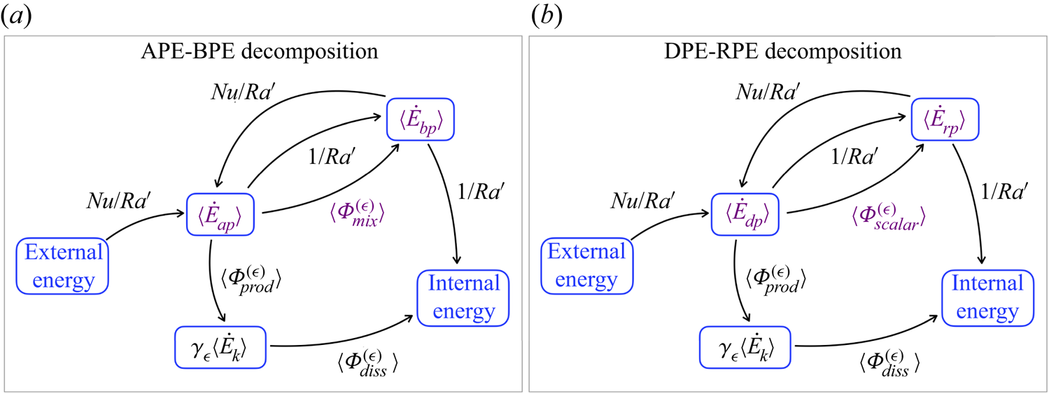
 $\textrm {d} E_{\textit {bp}}/\textrm {d}t$ and shown in figure 2.
Topology of the energy pathways in RBC for an incompressible Boussinesq fluid in a Hele-Shaw cell. We use the notation  $\gamma _{\epsilon } = \epsilon ^2 Ra'/Pr$, and
 $\dot {\langle\, f \rangle } = \textrm {d}\langle\, f \rangle /\textrm {d}t$ to denote the time derivative of the function
 $f$. (a) APE and BPE decomposition (APE–BPE). (b) DPE and RPE decomposition (DPE–RPE). Despite both energy pathways being similar, the potential reference states
 $\langle E_{\textit {bp}} \rangle$ and
 $\langle E_{\textit {rp}} \rangle$ are physically different. For the particular problem of RBC, the DPE–RPE decomposition allows computation of the energetics readily, without requiring
 $z_{\star }$ and its derivatives.

For the HS-RBC problem, let us now consider the evolution equation for the temperature fluctuations  $\sigma ^2 = \langle T^2 \rangle - \langle T \rangle ^2$ given by
 \begin{equation} \frac{1}{2}\,\frac{\textrm{d} \sigma^2 }{\textrm{d}t} + F^{(\textit{surf})}_{\sigma} ={-} \langle\varPhi_{\textit{scalar}}^{(\epsilon)}\rangle . \end{equation}
Thus, noticing that  $\langle T \rangle = 1/2$, one can link mathematically
 $\langle E_{\textit {rp}}\rangle$ and
 $\sigma ^{2}$ as follows:
 \begin{equation} \langle E_{\textit{rp}}\rangle ={-}\frac{1}{2}\, \sigma^2 - \frac{1}{8};\quad \frac{\textrm{d} \langle E_{\textit{rp}}\rangle}{\textrm{d}t} ={-}\frac{1}{2}\,\frac{\textrm{d} \sigma^2 }{\textrm{d}t} ={-}\frac{{\textit{Nu}}}{{\textit{Ra}}'} + \langle\varPhi_{\textit{scalar}}^{(\epsilon)}\rangle . \end{equation}
Since the destruction rate of the temperature variance,  $\langle \varPhi _{\textit {scalar}}^{(\epsilon )} \rangle$, is a natural metric of the rate at which thermal mixing occurs (Hidalgo et al. Reference Hidalgo, Fe, Cueto-Felgueroso and Juanes2012; Paoli et al. Reference Paoli, Giurgiu, Zonta and Soldati2019; Caulfield Reference Caulfield2021), the physical meaning of
 $\langle E_{\textit {rp}}\rangle$ is related to the ‘state of mixing’ of the system at a given time. The above interpretation is further supported in § 4, where we provide the explicit linear relationship between
 $\langle E_{\textit {rp}}\rangle$ and the degree of mixing
 $\chi$ introduced by Jha, Cueto-Felgueroso & Juanes (Reference Jha, Cueto-Felgueroso and Juanes2011), which is function of
 $\sigma ^2$. Under SSS conditions, the DPE–RPE decomposition does not change the energy pathways of HS-RBC because of the identity
 $\langle \varPhi _{\textit {mix}}^{(\epsilon )}\rangle _{\tau } = \langle \varPhi _{\textit {scalar}}^{(\epsilon )}\rangle _{\tau }$. However,
 $\langle E_{\textit {bp}}\rangle$ and
 $\langle E_{\textit {rp}}\rangle$ are physically different. Both
 $\langle E_{\textit {bp}}\rangle$ and
 $\langle E_{\textit {rp}}\rangle$ can be considered gauge fixing terms of a potential energy decomposition; the former is based on the state of minimum potential energy, whereas the latter is based on the state of mixing of the system. At SSS conditions, (3.22a,b) yields that
 $\langle {\textit {Nu}}\rangle _{\tau } = {\textit {Ra}}'\langle \varPhi _{\textit {scalar}}^{(\epsilon )}\rangle _{\tau }$, which reflects a balance between the surface buoyancy flux,
 $ {\textit {Nu}}/ {\textit {Ra}}'$, and its conversion into
 $\langle E_{\textit {rp}}\rangle$ via irreversible mixing at a rate
 $\langle \varPhi _{\textit {scalar}}^{(\epsilon )}\rangle$.
Here, we formulate the dynamic potential energy  $\langle E_{\textit {dp}}\rangle$ as the departure of the system's potential energy from its scalar fluctuations. From (3.6) and (3.22a,b), the evolution equation for the dynamic potential energy is given by
 \begin{equation} \frac{\textrm{d} \langle E_{\textit{dp}}\rangle}{\textrm{d}t} = 2\,\frac{{\textit{Nu}}}{{\textit{Ra}}'} - \left(\langle\varPhi_{\textit{prod}}^{(\epsilon)}\rangle + \langle\varPhi_{\textit{scalar}}^{(\epsilon)}\rangle + \frac{1}{{\textit{Ra}}'}\right). \end{equation}
For SSS conditions, i.e.  $\langle \textrm {d}\langle E_{\textit {dp}}\rangle /\textrm {d}t\rangle _{\tau } = 0$, the Nusselt number can then be expressed as
 $\langle {\textit {Nu}}\rangle _{\tau } = (1/2) {\textit {Ra}}'(\langle \varPhi _{\textit {diss}}^{(\epsilon )}\rangle _{\tau } + \langle \varPhi _{\textit {scalar}}^{(\epsilon )}\rangle _{\tau } + 1/ {\textit {Ra}}')$. The latter relation represents a fundamental balance between the continuous supply of energy at the boundaries and its rate of conversion into ‘internal energy’,
 $\langle \varPhi _{\textit {int}}^{(\epsilon )}\rangle _{\tau } = \langle \varPhi _{\textit {diss}}^{(\epsilon )}\rangle _{\tau } + \langle \varPhi _{\textit {scalar}}^{(\epsilon )}\rangle _{\tau } + 1/ {\textit {Ra}}'$, which is the total irreversible energy flux in the system due to small-scale processes. As we show later in § 4, the energy flux
 $\langle \varPhi _{\textit {int}}^{(\epsilon )}\rangle _{\tau }$ is important for the definition of efficiencies in HS-RBC.
Before proceeding, it is relevant to clarify the mathematical relationship between the APE–BPE and DPE–RPE formalisms. From (3.13) and (3.22a,b), we find that
 \begin{equation} \frac{\textrm{d}}{{\textrm{d}t}}\left(\langle E_{\textit{bp}}\rangle - \langle E_{\textit{rp}}\rangle\right) = \langle \varPhi^{(\epsilon)}_{\textit{mix}} \rangle - \langle \varPhi^{(\epsilon)}_{\textit{scalar}} \rangle. \end{equation}
Also, since the APE–BPE and DPE–RPE decompositions allow us to express the mean potential energy as  $\langle E_{\textit {p}} \rangle = \langle E_{\textit {ap}} \rangle + \langle E_{\textit {bp}} \rangle = \langle E_{\textit {dp}} \rangle + \langle E_{\textit {rp}} \rangle$, the latter identity and (3.24) lead to the following relationship:
 \begin{equation} \frac{\textrm{d}}{{\textrm{d}t}}\left(\langle E_{\textit{ap}}\rangle - \langle E_{\textit{dp}}\rangle\right) = \langle \varPhi^{(\epsilon)}_{\textit{scalar}} \rangle- \langle \varPhi^{(\epsilon)}_{\textit{mix}} \rangle. \end{equation}
Under SSS conditions, and using (3.17), the balance (3.25) satisfies
 \begin{equation} \bigg\langle\frac{\textrm{d}}{{\textrm{d}t}}\left(\langle E_{\textit{ap}}\rangle - \langle E_{\textit{dp}}\rangle\right)\bigg\rangle_{\tau} = 0 . \end{equation}
For fixed  $\epsilon$,
 $ {\textit {Ra}}'$ and
 $Pr$, a solution of (3.26) is
 \begin{equation} \langle E_{\textit{ap}}\rangle(t) = \langle E_{\textit{dp}}\rangle(t) + K + \varTheta(t), \end{equation}
with  $K$ a constant and
 $\varTheta (t)$ a function that satisfies
 $\langle \varTheta (t) \rangle _{\tau }=0$ and
 $\langle \textrm {d}\varTheta (t)/\textrm {d}t \rangle _{\tau } = 0$. The constant
 $K$ in (3.27) can be obtained by analysing the conductive regime, i.e.
 $ {\textit {Ra}} < 4{\rm \pi} ^2$. For the above, let us consider the definitions of
 $\langle E_{\textit {ap}} \rangle$ and
 $\langle E_{\textit {dp}} \rangle$ in (3.7a,b) and (3.20), respectively. Hence, for the conductive – non-convective – regime
 $\langle E_{\textit {ap}}\rangle _{\tau } = 1/6$ and
 $\langle E_{\textit {dp}}\rangle _{\tau } = 0$, i.e. (3.27) satisfies
 \begin{equation} \langle E_{\textit{ap}}\rangle_{\tau}=\langle E_{\textit{dp}}\rangle_{\tau} + \tfrac{1}{6}. \end{equation}
Thus, expressions (3.27) and (3.28) define the mathematical relationship between the APE–BPE and DPE–RPE formalisms. Hereinafter, we use the DPE–RPE decomposition to characterise the energetics and energy pathways of HS-RBC.
3.6. Energy pathways in HS-RBC
Figure 2 summarises the energy pathways of HS-RBC. The net heat supplied at the boundaries is converted into  $\langle E_{\textit {dp}}\rangle$ at rate
 $(2/Ra') {\textit {Nu}}$. When the dynamic potential energy is large enough to generate hydrodynamic instabilities,
 $ {\textit {Ra}}> 4{\rm \pi} ^{2}$ (Kimura, Schubert & Straus Reference Kimura, Schubert and Straus1986),
 $ {\textit {Nu}}$ becomes greater than unity. This means that the system shifts from a conductive to a convective regime, and finger-like thermal plumes start to produce kinetic energy at rate
 $\langle \varPhi ^{(\epsilon )}_{\textit {prod}}\rangle$ (figure 2a). The production is controlled by buoyancy-driven motions and dispersion. The onset of convection not only generates fluid displacement that enhances vertical heat transport, but also boosts dissipative mechanisms. Thus, kinetic energy is dissipated and converted into internal energy due mainly to Darcy friction at rate
 $\langle \varPhi ^{(\epsilon )}_{\textit {diss}} \rangle$ (figure 2a). As a consequence of stretching and squeezing of the isotherms, the remaining dynamic potential energy is expended in irreversible thermal mixing at rate
 $\langle \varPhi ^{(\epsilon )}_{\textit {scalar}}\rangle +1/Ra'$ (figure 2b).
Summarising our results for HS-RBC, the energetics are determined by the Nusselt and Rayleigh numbers as follows:
 \begin{equation} \langle\varPhi^{(\epsilon)}_{\textit{prod}}\rangle_{\tau} = \frac{1}{Ra'}\left(\langle {\textit{Nu}}\rangle_{\tau}-1\right);\quad \langle \varPhi^{(\epsilon)}_{\textit{scalar}}\rangle_{\tau} = \frac{\langle {\textit{Nu}}\rangle_{\tau}}{Ra'}; \quad \langle \varPhi^{(\epsilon)}_{\textit{int}}\rangle_{\tau} = 2\frac{\langle {\textit{Nu}}' \rangle_{\tau}}{{\textit{Ra}}'}. \end{equation}
4. Efficiencies and degree of mixing
We use three metrics to link the energy partition with the heat transport and mixing in HS-RBC under statistically steady conditions. First, we define the ‘convective efficiency’  $\eta _c$ as the fraction of dynamic potential energy,
 $\langle E_{\textit {dp}} \rangle$, expended in driving motion
 \begin{equation} \eta_c=\frac{\langle\varPhi_{\textit{prod}}^{(\epsilon)}\rangle_{\tau}}{\langle\varPhi_{\textit{int}}^{(\epsilon)}\rangle_{\tau}}. \end{equation}
Using the results in (3.29a–c), the convective efficiency can be expressed as
 \begin{equation} \eta_c = \frac{1}{2}\left(1 - \frac{1}{\langle{\textit{Nu}}\rangle_{\tau}}\right), \end{equation}
where  $\langle {\textit {Nu}}\rangle _{\tau }$ quantifies the global heat transfer. For conductive regimes,
 $\langle {\textit {Nu}}\rangle _{\tau } = 1$, the energy consumed in transporting heat by convection becomes null,
 $\eta _{c} = 0$. By contrast, when the primary transport mechanism is convection, i.e.
 $\langle {\textit {Nu}}\rangle _{\tau } \gg 1$,
 $\eta _{c}\rightarrow 1/2$.
The second metric is the ‘mixing efficiency’ (Davies Wykes et al. Reference Davies Wykes, Hughes and Dalziel2015; Caulfield Reference Caulfield2020), defined as
 \begin{equation} \eta_m = \frac{\langle\varPhi^{(\epsilon)}_{\textit{scalar}}\rangle_{\tau}+1/Ra'}{\langle\varPhi^{\epsilon}_{\textit{int}}\rangle_{\tau}}. \end{equation}
Using the results in (3.29a–c), the mixing efficiency can be expressed as
 \begin{equation} \eta_m = \frac{1}{2}\left(1 +\frac{ 1}{\langle{\textit{Nu}}\rangle_{\tau}}\right), \end{equation}
and it quantifies the fraction of  $\langle E_{\textit {dp}} \rangle$ expended in thermal mixing. For 3D-RBC, Hughes et al. (Reference Hughes, Gayen and Griffiths2013) derived the same expression in (4.4) using the APE–BPE decomposition. Notice that (4.2) and (4.4) satisfy
 $\eta _{m}+\eta _{c}=1$ and that for
 $\langle {\textit {Nu}}\rangle _{\tau } \gg 1$, both efficiencies are asymptotically convergent to
 $1/2$. As in 3D-RBC, the mixing efficiency in Hele-Shaw geometries is only governed by the Nusselt number.
The third metric is the ‘degree of mixing’ of the system (Jha et al. Reference Jha, Cueto-Felgueroso and Juanes2011), defined as
 \begin{equation} \chi = 1-12\sigma^2, \end{equation}
where  $\chi = 1$ represents a perfectly mixed state and
 $\chi = 0$ represents a perfectly segregated state. Thus,
 $\chi$ provides information about the inner thermal state of the bulk. Notice that we can express the reference potential energy as a function of the degree of mixing as
 \begin{equation} \langle E_{\textit{rp}}\rangle = \chi/24 -1/6. \end{equation}
The latter identity provides a physical argument to link  $\langle E_{\textit {rp}}\rangle$ with the state of mixing of a system.
5. Numerical experiments
We performed a series of direct numerical simulations of the Hele-Shaw model (2.2) to: (i) illustrate the spatial and temporal structure of the energetics introduced in § 3; (ii) compare the numerical estimation of the convective efficiency  $\eta _{c}$ obtained from (4.1) with the analytical result in (4.2); and (iii) explore the degree of mixing (4.5) as a function of the Rayleigh number.
5.1. Numerical implementation
The numerical experiments were performed using the spectral solver flow  $\_$ solve (Winters & de la Fuente Reference Winters and de la Fuente2012), which has been applied for a wide range of geophysical fluid dynamics problems (e.g. Barkan, Winters & Llewellyn Smith Reference Barkan, Winters and Llewellyn Smith2013; Letelier et al. Reference Letelier, Mujica and Ortega2019; Ulloa et al. Reference Ulloa, Winters, Wüest and Bouffard2019).
The dynamical variables in (2.2a) were expanded by means of trigonometric basis functions over the rectangular (Hele-Shaw) computational domain and integrated in time using a third-order Adams–Bashforth scheme for advective/buoyant terms and the implicit fourth-order Adams–Moulton method for diffusive scheme. The equations of motion admitted a base state solution given by  $u_s = 0$,
 $w_s = 0$,
 $T_s(z) = 1 - z$ and
 $p_s(z) = p_0 + \int _{0}^{z} T_s(\xi )\,\textrm {d}\xi$. Then, we perturbed all dynamical variables as
 $u(t,\boldsymbol {x}) = u'(t,\boldsymbol {x})$,
 $w(t,\boldsymbol {x}) = w'(t,\boldsymbol {x})$,
 $p(t,\boldsymbol {x}) = p_s(z) + p'(t,\boldsymbol {x})$ and
 $T(t,\boldsymbol {x}) = T_s(z) + \theta (t,\boldsymbol {x})$. From the boundary conditions defined in figure 1, we expanded
 $u' \sim \exp (\textrm {i}k_n x)\cos (n{\rm \pi} z)$,
 $w' \sim \exp (\textrm {i}k_nx)\sin (n{\rm \pi} z)$,
 $p' \sim \exp (\textrm {i}k_nx)\cos (n{\rm \pi} z)$ and
 $\theta \sim \exp (\textrm {i}k_nx)\sin (n{\rm \pi} z)$, with
 $n$ a natural number and
 $k_n$ the wavenumber.
The spatial resolution  $\Delta x=\Delta z$ was chosen to resolve at least with ten grid points the thermal and viscous boundary layers, a priori estimated as
 $\delta _{T}/H\sim {\textit {Ra}}^{-1/3}$ and
 $\delta _{u}/H\sim (Pr/ {\textit {Ra}})^{-1/2}$, respectively (Ahlers et al. Reference Ahlers, Grossmann and Lohse2009b). The time step was defined satisfying the Courant–Friedrichs–Lewy (CFL) condition of the numerical scheme,
 $\textrm {CFL}\leqslant 0.2$, for both velocity components.
The numerical procedure to compute the horizontal average of a function  $f_i = f(x_i)$ over
 $n_{x}$ grid points was based on a cubic spline interpolation of
 $f$ on a three times denser grid, with
 $m_x = 3n_x$ points. The new interpolated function
 $f^{new}_{j}$, with
 $j = 1,\ldots,m_x$, was integrated using the composite Simpson rule. The same procedure was used for the domain average of a function in the vertical direction. Numerical derivatives were computed using a spectral approach based on Fourier, sine and cosine transforms, depending on the boundary conditions.
Despite the highly accurate numerical schemes used, numerical diffusion problems arose mainly from the numerical averaging procedure, which was not sufficiently accurate to preserve the same numerical precision of the spectral methods. Thus, it was not possible to recover numerically the condition  $\langle \textrm {d} \langle E_{\textit {f}}\rangle /\textrm {d}t\rangle _{\tau } = 0$ for
 ${\textit {f}} = \{\textit {k},\textit {rp},\textit {dp}\}$ the indices to denote the mechanical energy components. For the cases analysed in this manuscript, we obtained
 $\langle \textrm {d} \langle E_{\textit {f}}\rangle /\textrm {d}t\rangle _{\tau } = \delta _{\textit {f}} \lesssim O(\epsilon ^2)$, with
 $O(\epsilon ^2)$ the order of magnitude of the smallest contribution in the energy budgets. Nevertheless, the latter gave an adequate accuracy to resolve the mechanical energy budget for the RBC problem in Hele-Shaw cells, so the numerical deviations
 $\delta _{\textit {f}}$ were treated as numerical errors. To propagate the errors, we defined the following energy rates:
 $\langle \varPhi _{\textit {prod}}^{(\epsilon )}\rangle ^{*}_{\tau } = \langle \varPhi _{ \textit {prod}}^{(\epsilon )}\rangle _{\tau } \pm \delta _{\textit {k}}$,
 $\langle \varPhi _{diss}^{(\epsilon )}\rangle ^{*}_{\tau } = \langle \varPhi _{diss}^{(\epsilon )}\rangle _{\tau } \pm \delta _{\textit {k}}$,
 $\langle \varPhi _{\textit {scalar}}^{(\epsilon )}\rangle ^{*}_{\tau } = \langle \varPhi _{\textit {scalar}}^{(\epsilon )}\rangle _{\tau } \pm \delta _{\textit {r}}$ and
 $\langle {\textit {Nu}}\rangle ^{*}_{\tau }/ {\textit {Ra}}' = \langle {\textit {Nu}}\rangle _{\tau }/ {\textit {Ra}}' \pm \delta _{\textit {r}}$. Therefore, the convective efficiency was computed as
 $\eta _c^{*} = \eta _c \pm \delta _{\eta }$, with
 $\delta _{\eta } = (\delta _{\textit {k}}/\langle \varPhi ^{(\epsilon )}_{\textit {int}}\rangle _{\tau })\,\sqrt {1 + \eta _c^2\,[(\delta _{\textit {k}} + \delta _{\textit {r}})/\delta _k]^2}$.
To estimate the APE and the diapycnal mixing rate  $\langle \varPhi ^{(\epsilon )}_{\textit {mix}}\rangle$ introduced in § 3.3, we computed
 $z_{\star }(T)$ following the algorithm given by Winters & Barkan (Reference Winters and Barkan2013). In order to obtain
 $\textrm {d}z_{\star }/\textrm {d}T$, we smoothed
 $z_{\star }$ using a linear interpolation on a grid
 $n^{(1)}_g = n_g/100$, with
 $n_g = n_{x}\times n_z$ the original numerical length vector for
 $z_{\star }$. This procedure allowed us to build the new function
 $z^{(1)}_{\star }$. Then, we built a high-resolution representation of the smoothed
 $z^{(1)}_{\star }$ applying a cubic interpolation on a grid
 $n^{(2)}_g = 50\times n^{(1)}_g = n_g/2$, generating the final function
 $z^{(2)}_{\star }$. The derivative
 $\textrm {d}z_{\star }/\textrm {d}T$ was computed from
 $z^{(2)}_{\star }$ using compact finite differences (Lele Reference Lele1992). The obtained result was smoothed using a low-pass filter based on the FFT transform of the odd extension of
 $\textrm {d}z_{\star }/\textrm {d}T$.
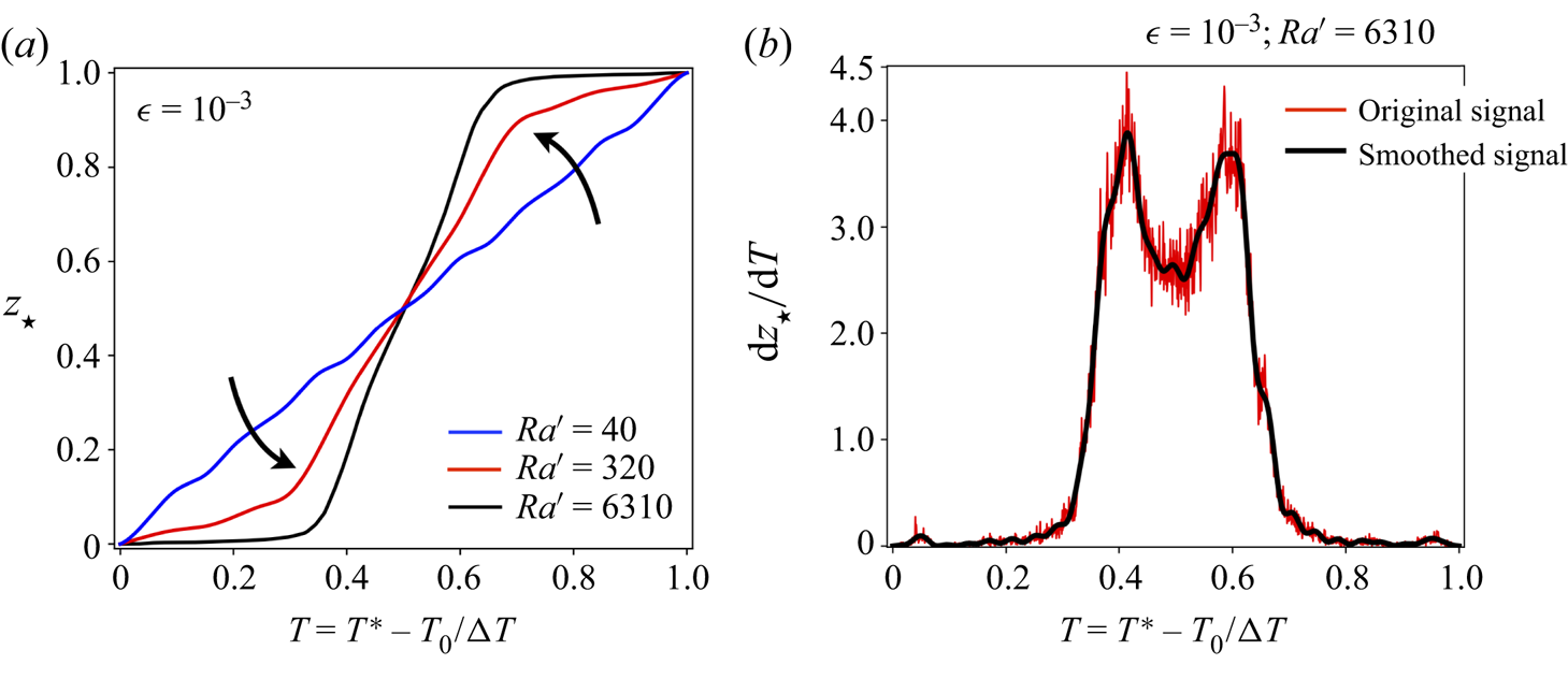
As an example, figure 3 illustrates  $z_{\star }$ and
 $\textrm {d}z_{\star }/\textrm {d}T$ as a function of the temperature field
 $T$ for a numerical experiment characterised by
 $\epsilon =10^{-3}$ and
 $ {\textit {Ra}}=7527$. Consistently, we observe that
 $z_{\star }$ is a monotonically increasing function of
 $T$, with
 $z_{\star }(T=0)=0$ and
 $z_{\star }(T=1)=1$. Its derivative is a positive, nonlinear function of
 $T$. As we show later in § 5.2, the interpolation and smoothing procedure to compute
 $\textrm {d}z_{\star }/\textrm {d}T$,
 $\langle \varPhi ^{(\epsilon )}_{\textit {mix}} \rangle _{\tau }$ and (3.18), gives absolute values of
 $\varDelta _{\textit {mix}} \sim 10^{-4}$ for high-
 $ {\textit {Ra}}$, which is approximately
 $1\,\%$ of
 $\langle \varPhi ^{(\epsilon )}_{\textit {scalar}} \rangle _{\tau }$. For low-
 $ {\textit {Ra}}$, however,
 $\varDelta _{\textit {mix}} \sim 10^{-5}$. These are our best values obtained from the methodology discussed above.
(a) Shows the reference state  $z_{\star }$ of fluid parcels at their gravitational equilibrium with respect to the temperature field
 $T$ for
 $\epsilon =10^{-3}$ and three Rayleigh numbers at SSS conditions. As
 $ {\textit {Ra}}$ increases, the function
 $z_{\star }(T)$ departures from its initial state condition
 $z_{\star }=T$ to achieve new distributions at SSS conditions, which tend towards the homogenisation of the inner temperature field while keeping the boundary conditions
 $z_{\star }(0)=0$ and
 $z_{\star }(1)=1$. (b) Shows the derivative of
 $z_{\star }$ with respect to
 $T$ as a function of
 $T$ for
 $\epsilon =10^{-3}$ and
 $ {\textit {Ra}}=7572$ at SSS conditions. A low-pass filter based on the fast Fourier transform (FFT) was applied, with a cutoff wavenumber of
 $50{\rm \pi} /L$, with
 $L=1$ the amplitude of the dimensionless temperature.

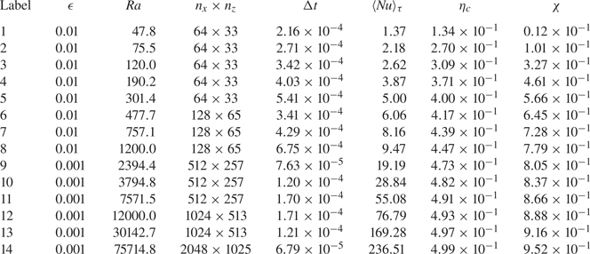
Our simulations considered  $4.7\times 10^{1} \leqslant {\textit {Ra}} \leqslant 7.5\times 10^{4}$, with
 $Pr = 7$ and two values of the anisotropy ratio,
 $\epsilon =10^{-3}$ and
 $\epsilon =10^{-2}$. The experimental set is summarised in table 1.
Parameter space and resolution of numerical experiments presented in figures 4 and 8. The non-dimensional grid spatial resolutions in  $x$ and
 $z$ are
 $\varDelta _{x} = L'/n_{x}$ and
 $\varDelta _{z} = 1/(n_{z}-1)$, respectively, while the non-dimensional time step is
 $\Delta t$. The cell aspect ratio
 $L' = L_x/L_z = 2$ and the Prandtl number
 $Pr=7$ were kept constant for all our experiments. In this table, the values of
 $\eta _c$ are computed using (4.1).

5.2. Results
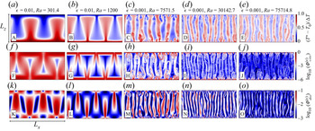
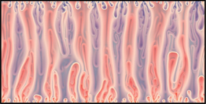
Figure 4 shows the non-dimensional temperature,  $\varPhi ^{(\epsilon )}_{\textit {scalar}}$ and
 $\varPhi ^{(\epsilon )}_{\textit {diss}}$ fields for different
 $\epsilon$ and
 $ {\textit {Ra}}$. For
 $4{\rm \pi} ^{2}< {\textit {Ra}}<1350$ and SSS conditions, the above fields show coherent convective structures (figure 4a,b). For
 $ {\textit {Ra}}\geqslant 1350$ and SSS conditions, on the other hand, convection becomes chaotic, and the flow is self-organised into ‘multi-megaplumes’ (figure 4c–e). Figure 4(f–j) shows that thermal mixing rates are maximal at the boundaries of convective plumes, where isotherms tend to squeeze due to the thermals’ development – the higher rates of
 $\varPhi ^{(\epsilon )}_{\textit {scalar}}$ occur near the top and bottom boundaries. We remark that, as
 $Ra$ increases, the zone over which the maximum rates are found becomes more confined near the horizontal boundaries. In contrast, figure 4(k–o) shows that the kinetic energy dissipation rate,
 $\varPhi ^{(\epsilon )}_{\textit {diss}}$, has its higher magnitudes in the interior zone, spatially aligned throughout the core of the megaplumes. As
 $Ra$ increases, the maximum dissipation rates tend to become scattered and weaker.
Results of numerical experiments of the Hele-Shaw model (2.2) for five different  $\epsilon$ and
 $ {\textit {Ra}}$ values under SSS conditions. All quantities are in non-dimensional units. (a–e) Show the temperature fields in the Hele-Shaw domain (
 $x$–
 $z$ plane). (f–j) Show the scalar dissipation rate
 $\varPhi ^{(\epsilon )}_{\textit {scalar}}$, where their maximum values are achieved along the boundaries of thermal plumes. (k–o) Show the dissipation rate
 $\varPhi ^{(\epsilon )}_{\textit {diss}}$;
 $\varPhi ^{(\epsilon )}_{\textit {diss}}$ achieves maximum values inside the core of each thermal plume, where the Darcy induced dissipation is dominant. Inset labels A–O link these results with the results in figure 8.

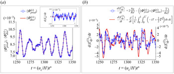
Figure 5 illustrates mean energetic quantities as a function of time for  $\epsilon = 10^{-3}$ and
 $ {\textit {Ra}} = 7571.5$, under SSS conditions. Figure 5(a) shows times series of the energetics involved in the mean kinetic energy balance,
 $\langle \varPhi ^{(\epsilon )}_{\textit {prod}}\rangle$ and
 $\langle \varPhi ^{(\epsilon )}_{\textit {diss}}\rangle$. The production rate of kinetic energy is balanced by its dissipation rate. The latter is further corroborated by the inset panel in figure 5(a), which shows that the rate of change in time of the mean kinetic energy is statistically zero. Figure 5(b), on the other hand, shows the rate of change in time of the dynamic potential energy component,
 $\textrm {d}\langle E_{\textit {dp}}\rangle /\textrm {d}t$. The above quantity was computed following two approaches. First, we computed
 $\textrm {d}\langle E^{(1)}_{\textit {dp}}\rangle /\textrm {d}t$ directly from the energetics on the right-hand side of (3.23). Second, we computed the rate of change in time of
 $\langle E_{\textit {dp}}\rangle$ from (3.20), i.e.
 $\textrm {d}\langle E^{(2)}_{\textit {dp}}\rangle /\textrm {d}t$. In both cases,
 $\textrm {d}\langle E_{\textit {dp}}\rangle /\textrm {d}t$ exhibits an oscillatory dynamics around zero at high-
 $ {\textit {Ra}}$ and a statistically steady regime.
Results of experiment 11 under SSS conditions,  $\epsilon = 10^{-3}$ and
 $ {\textit {Ra}} = 7571.5$. All quantities are in non-dimensional units. (a) Shows the mean kinetic energy production rate
 $\langle \varPhi ^{(\epsilon )}_{\textit {prod}}\rangle$ and the mean kinetic dissipation rate
 $\langle \varPhi ^{(\epsilon )}_{\textit {diss}}\rangle$ as functions of time
 $t$. The inset in (a) exhibits the time derivative of the mean kinetic energy
 $\langle E_{\textit {k}}\rangle$, oscillating around zero, i.e.
 $\langle \textrm {d}\langle E_{\textit {k}}\rangle /{\textrm {d}t}\rangle _{\tau }=0$. (b) Shows times series of the rate of change in time of the dynamic potential energy,
 $\textrm {d}\langle E_{\textit {dp}}\rangle /\textrm {d}t$, computed from the energetics (left vertical axis) and from the rate of change in time of
 $\langle E_{\textit {dp}} \rangle$ defined in (3.20) (right vertical axis). Both estimations follow the same temporal pattern and oscillate around zero, i.e.
 $\langle \textrm {d}\langle E_{\textit {dp}}\rangle /{\textrm {d}t}\rangle _{\tau }=0$.

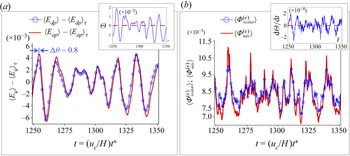
Figure 6 illustrates the relationship between the mean dynamic potential energy,  $\langle E_{\textit {dp}}\rangle$, and the mean APE,
 $\langle E_{\textit {ap}}\rangle$. Figure 6(a) displays time series of
 $\langle E_{\textit {dp}}\rangle (t)-\langle E_{\textit {dp}}\rangle _{\tau }$ and
 $\langle E_{\textit {ap}}\rangle (t)-\langle E_{\textit {ap}}\rangle _{\tau }$. As expected for SSS conditions – see (3.26) and (3.27) – both quantities should differ from a constant and a time-dependent function
 $\varTheta (t)$, exhibited in the inset panel. We highlight the similitude (as a function of time) between both quantities and that their rate of change in time is statistically the same, as shown in (3.25). The rate of change of the APE depends on the irreversible mixing rate
 $\langle \varPhi ^{(\epsilon )}_{\textit {mix}} \rangle$, displayed as a function of time in figure 6(b). On the other hand, the rate of change of the dynamic potential energy depends on the thermal dissipation rate
 $\langle \varPhi ^{(\epsilon )}_{\textit {scalar}}\rangle$, also displayed as a function of time in figure 6(b). The graph shows that
 $\langle \varPhi ^{(\epsilon )}_{\textit {mix}}\rangle$ and
 $\langle \varPhi ^{(\epsilon )}_{\textit {scalar}}\rangle$ follow the same pattern and magnitude, with minor differences that may result from the adopted numerical procedure to compute
 $\textrm {d}z_{\star }/\textrm {d}T$. The result in figure 6(b) supports numerically that, at SSS conditions, the relationship
 $\langle \varPhi ^{(\epsilon )}_{\textit {mix}} \rangle _{\tau } =\langle \varPhi ^{(\epsilon )}_{\textit {scalar}} \rangle _{\tau }$ is fulfilled, with a numerical absolute difference (error) of
 $\varDelta _{\textit {mix}} \sim 10^{-4}$ and a relative difference of approximately 1 % with respect to
 $\langle \varPhi ^{(\epsilon )}_{\textit {scalar}} \rangle _{\tau }$. Additionally, the inset panel in figure 6(b) exhibits the rate of change in time of
 $\varTheta$, which shows a fluctuating pattern with a mean temporal value of approximately zero. The latter is required to characterise the functional relationship between
 $\langle E_{\textit {ap}}\rangle (t)$ and
 $\langle E_{\textit {dp}}\rangle (t)$ introduced in (3.27).
Results of experiment 11 under SSS conditions,  $\epsilon = 10^{-3}$ and
 $ {\textit {Ra}} = 7571.5$. All quantities are in non-dimensional units. (a) Shows the temporal evolution of the mean dynamic potential energy
 $\langle E_{\textit {dp}} \rangle$ and the mean available potential energy,
 $\langle E_{\textit {ap}} \rangle$, as functions of time
 $t$. Both potential energy components are defined relative to their time averages
 $\langle E_{\textit {dp}}\rangle$ and
 $\langle E_{\textit {ap}}\rangle$, respectively. The inset in (a) exhibits the function
 $\varTheta (t)=\langle E_{\textit {ap}}\rangle (t)-\langle E_{\textit {dp}}\rangle (t)-(\langle E_{\textit {ap}}\rangle _{\tau }-\langle E_{\textit {dp}}\rangle _{\tau })$, which fluctuates around zero, i.e.
 $\langle \varTheta \rangle _{\tau }=0$. (b) Shows times series of the rate of change in time of the scalar dissipation rate
 $\langle \varPhi ^{(\epsilon )}_{\textit {scalar}}\rangle$ and the diapycnal mixing rate
 $\langle \varPhi ^{(\epsilon )}_{\textit {mix}}\rangle$ as functions of time
 $t$. Both quantities follow the same temporal pattern and have the same order of magnitude. The inset figure in (b) shows the rate of change in time of
 $\varTheta (t)$, which fluctuates around zero, i.e.
 $\langle \textrm {d}\varTheta /{\textrm {d}t}\rangle _{\tau }=0$.

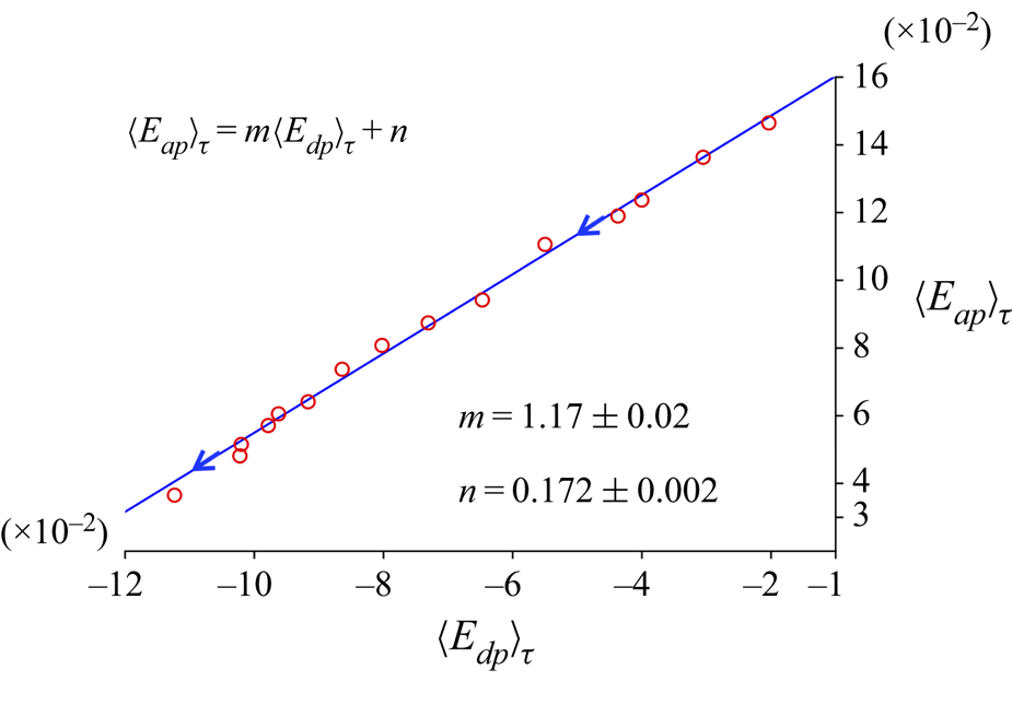
Under SSS conditions, the time-averaged mean available and dynamic potential energy components must fulfil the relationship  $\langle E_{\textit {ap}}\rangle _{\tau } =\langle E_{\textit {dp}}\rangle _{\tau } + K$ in (3.28), with
 $K=1/6$. Consistently, figure 7 shows that the numerical experiments agree with the latter identity; the slope
 $m$ of the linear fitting is approximately one in absolute value,
 $|m|\approx 1.17\pm 0.02$, and the intercept
 $n\approx K\approx 0.172\pm 0.002$. Differences between theory and the numerical results are not unexpected since they may well arise from the numerical procedure to compute integrals and averages.
Relationship between time-averaged mean available potential energy  $\langle E_{\textit {ap}}\rangle _{\tau }$ and time-averaged mean dynamic potential energy,
 $\langle E_{\textit {dp}}\rangle _{\tau }$, for the numerical experiments at SSS conditions (red circles). The linear least-square fitting
 $\langle E_{\textit {ap}} \rangle _{\tau }=m\langle E_{\textit {dp}} \rangle _{\tau }+n$ shows good agreement with the relationship (3.28). The arrow indicates the growth direction of
 $ {\textit {Ra}}$.

The relationship between the convective efficiency  $\eta _{c}$ and the global Nusselt number
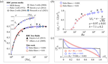
 $\langle {\textit {Nu}} \rangle _{\tau }$ is shown in figure 8(a). Using our numerical experiments, we confirm that, under SSS conditions, the convective and mixing efficiencies, (4.1) and (4.3), can be estimated by the expressions (4.2) and (4.4), respectively. The solid curve in the main panel illustrates the analytical expression for
 $\eta _{c}$ in (4.2), whereas markers derived from this figure (see legend) show
 $\eta _{c}$ computed numerically from (4.1). All points collapse to the analytical curve
 $\eta _{c}$–
 $\langle {\textit {Nu}} \rangle _{\tau }$. We identify that for
 $\langle {\textit {Nu}}\rangle _{\tau }=10$, already approximately 45 % of the available energy is used in transporting heat by convection. However, to reach values close to the maximum convective efficiency, i.e. when 50 % of the APE is used to produce convection,
 $\langle {\textit {Nu}} \rangle _{\tau }$ must increase by at least two orders of magnitude, as shown in the upper inset.
(a) Convective efficiency as a function of the global Nusselt number,  $\langle {\textit {Nu}}\rangle _{\tau }$. Solid curves in the main panel and magnified region correspond to the analytical convective efficiency as a function of
 $\langle {\textit {Nu}}\rangle _{\tau }$,
 $\eta _{c}=(1/2)(1-1/\langle {\textit {Nu}}\rangle _{\tau })$. Symbols for this figure (diamonds and circles) correspond to convective efficiencies computed numerically from the energetics,
 $\eta _{c}=\langle \varPhi ^{(\epsilon )}_{\textit {prod}}\rangle _{\tau }/\langle \varPhi ^{(\epsilon )}_{int}\rangle _{\tau }$. Convective efficiencies associated with symbols from previous studies of 2-D porous media and free fluids were obtained based on the Nusselt numbers reported and steady-state conditions, i.e.
 $\eta _{c}=(1/2)(1-1/\langle {\textit {Nu}}\rangle _{\tau })$. (b) Degree of mixing
 $\langle \chi \rangle _{\tau }$ as a function of
 $ {\textit {Ra}}$ and computed from the Hele-Shaw numerical experiments. (c) Horizontally averaged temperature distribution
 $\langle T \rangle _{h}$ as a function of height
 $z/L$ for three numerical experiments. For
 $Ra\geqslant 4{\rm \pi} ^{2}$, convection begins to govern the heat transport, and the horizontally averaged temperature field changes from a linear distribution as a function of height,
 $T_{s} = 1-z$ (red symbols), to an almost uniform distribution,
 $\langle T\rangle _h\approx 1/2$, in the interior as convection becomes vigorous and TBLs become thinner (black curve).

Figure 8(b) exhibits the ‘degree of mixing’  $\langle \chi \rangle _{\tau }$ as a function of
 $ {\textit {Ra}}$ computed from the numerical experiments summarised in table 1. The numerical results show that
 $\langle \chi \rangle _{\tau }$ follows the relationship
 \begin{equation} \langle\chi \rangle_{\tau} =\begin{cases} 0 & \mbox{if } Ra < 4{\rm \pi}^{2},\\ a - b\,Ra^{{-}1/2} & \mbox{if } Ra \geqslant 4{\rm \pi}^{2} , \end{cases} \end{equation}
with  $a=0.97\pm 0.01$ and
 $b=7.1\pm 0.2$. Expression (5.1) evidences a functional dependence between the level of the inner temperature homogenisation characterised by
 $\langle \chi \rangle _{\tau }$ and
 $ {\textit {Ra}}$. The fitting parameter ‘
 $a$’ indicates that at high-
 $ {\textit {Ra}}$, the degree of mixing
 $\langle \chi \rangle _{\tau }\rightarrow 1$. However, as shown in figure 8(c), the TBLs must match the temperature boundary conditions (figure 1), so
 $\chi$ cannot be exactly 1.
Furthermore, recalling that  $\chi$ allows determination of the RPE (see (4.6)), we can directly study the physics of RPE by looking at its response to variations on the state of mixing at SSS conditions,
 $\varDelta _{\chi }\langle E_{\textit {rp}}\rangle _{\tau } = (1/24)\varDelta \langle \chi \rangle _{\tau }$. Thus, if the system shifts from a conductive to a convective regime, i.e.
 $\varDelta \langle \chi \rangle _{\tau } > 0$, then the system ‘gains’ RPE due to a better homogenisation of the temperature scalar field.
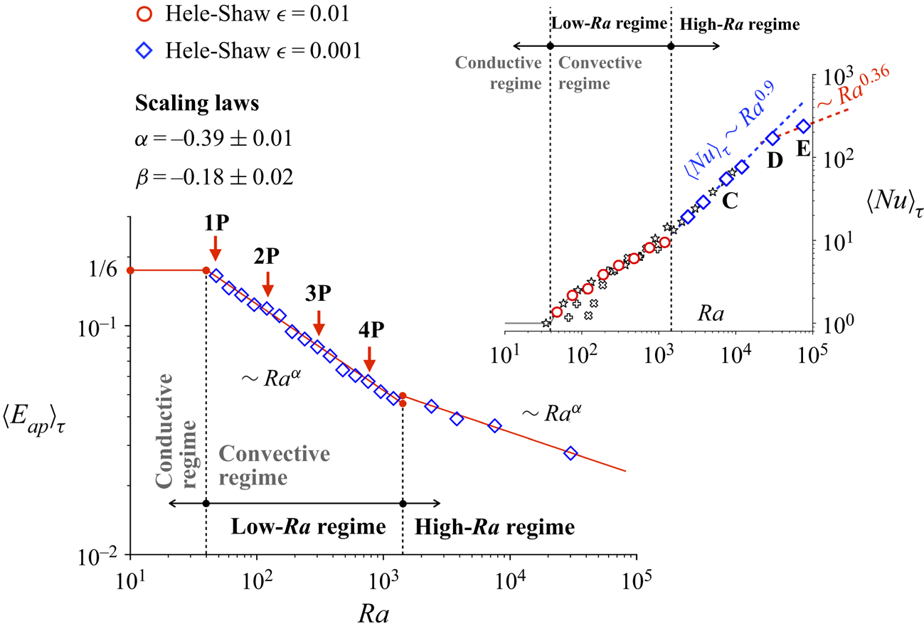
Figure 9 shows the scaling laws for  $\langle E_{\textit {ap}}\rangle _{\tau }$ and
 $\langle {\textit {Nu}} \rangle _{\tau }$ as functions of
 $ {\textit {Ra}}$. In the low-
 $ {\textit {Ra}}$ regime, i.e.
 $4{\rm \pi} ^2 \leqslant {\textit {Ra}} \leqslant 1350$;
 $\langle E_{\textit {ap}}\rangle _{\tau }$-
 $ {\textit {Ra}}$ shows a robust linear fitting in logarithmic scale, instead of the multiscale, complex relationship observed in
 $\langle {\textit {Nu}} \rangle _{\tau }$-
 $ {\textit {Ra}}$ (inset panel). In this regime,
 $\langle E_{\textit {ap}}\rangle _{\tau } \sim {\textit {Ra}}^{-0.38}$. An interesting finding is that the slope observed in
 $\langle E_{\textit {ap}}\rangle _{\tau }$-
 $ {\textit {Ra}}$ changes at
 $ {\textit {Ra}} \sim 1350$. This change is understood as a transition from fully steady-state conditions towards quasi-steady-state conditions, where chaotic multi-megaplumes govern the dynamics. The same change is also observed in
 $\langle {\textit {Nu}} \rangle _{\tau }$-
 $ {\textit {Ra}}$ (inset panel). Notice that the global Nusselt number and the Rayleigh number exhibit a power-law relationship
 $\langle {\textit {Nu}} \rangle _{\tau }\sim {\textit {Ra}}^{0.9}$ for
 $1350< {\textit {Ra}}<10^{4}$ (part of the high-
 $ {\textit {Ra}}$ regime). The latter is the same scaling law obtained for 2-D porous media by Hewitt et al. (Reference Hewitt, Neufeld and Lister2012). Yet the above power law changes at approximately
 $ {\textit {Ra}}=3\times 10^{4}$ for
 $\epsilon =0.001$, from where it is observed that
 $\langle {\textit {Nu}} \rangle _{\tau }\sim {\textit {Ra}}^{0.36}$.
Numerical results under SSS conditions. Time-averaged, mean APE,  $\langle E_{\textit {ap}}\rangle _{\tau }$, as a function of
 $ {\textit {Ra}} \leqslant 30\,000$. Inset plot shows the Nusselt number
 $\langle {\textit {Nu}}\rangle _{\tau }$ as a function of
 $ {\textit {Ra}}$. Results show that
 $\langle E_{\textit {ap}}\rangle _{\tau }$ scales with
 $ {\textit {Ra}}$ following a power law
 $ {\textit {Ra}}^{m}$, depending on the
 $ {\textit {Ra}}$ regime, i.e.
 $m = -0.39$ for
 $4{\rm \pi} ^2 \leqslant {\textit {Ra}} \leqslant 1350$ (the low-
 $ {\textit {Ra}}$ regime), whilst
 $m = -0.18$ for
 $1350 < {\textit {Ra}} \leqslant 30\,000$ (part of the high-
 $ {\textit {Ra}}$ regime). Labels 1P to 4P indicate the number of steady-state plumes in the Hele-Shaw cell for low-
 $Ra$ regime.

6. Discussion
6.1. The Nusselt and Rayleigh numbers
As shown in § 3.6, under SSS conditions, the energetics of HS-RBC are determined by both the global Nusselt number  $\langle {\textit {Nu}}\rangle _{\tau }$ and the Rayleigh number of the system, whereas the efficiencies
 $\eta _{c}$ and
 $\eta _{m}$ introduced in § 4 only depend on
 $\langle {\textit {Nu}}\rangle _{\tau }$. Owing to these results, determining general scaling laws for the Nusselt number would allow us to quantify the energetics and the efficiencies of RBC from external parameters only. In order to generalise our results, future studies should look at the transition from HS-RBC to 3D-RBC. Yet one of the first challenges we face is the lack of a unified definition for the system's Rayleigh number.
In environments where RBC is ‘free’ to develop fully 3-D structures, convection transfers heat and energy throughout the three spatial dimensions. For these cases, the Rayleigh number is traditionally defined as  $ {\textit {Ra}}_{*} = (\alpha \Delta T g H^3)/(\rho _{c}\kappa _{c}\nu _{c})$, and the power of the scaling law
 $\langle {\textit {Nu}}\rangle _{\tau } \sim {\textit {Ra}}_{*}^{\gamma }$ varies between
 $\gamma =0.14$ and
 $\gamma =0.38$, depending on
 $ {\textit {Ra}}_{*}$ and the dynamics of the TBLs (Ahlers et al. Reference Ahlers, Funfschilling and Bodenschatz2009a; Funfschilling, Bodenschatz & Ahlers Reference Funfschilling, Bodenschatz and Ahlers2009; Grossmann & Lohse Reference Grossmann and Lohse2011). However, for RBC in porous media (also known as Rayleigh–Darcy convection), the Rayleigh number (also known as the Rayleigh–Darcy number) is the same as that used here for Hele-Shaw geometries,
 $ {\textit {Ra}} = (\alpha \Delta T g K H)/(\rho _{c}\kappa _{c}\nu _{c})$. In 2-D convection in porous media, the scaling law between the Nusselt and Rayleigh numbers varies from
 $\langle {\textit {Nu}}\rangle _{\tau } \sim {\textit {Ra}}^{0.9}$ for
 $10^3 < Ra < 10^4$, to
 $\langle {\textit {Nu}} \rangle _{\tau } \sim {\textit {Ra}}$ for the ultimate regime, i.e.
 $ {\textit {Ra}} \gg 10^5$ (Doering & Constantin Reference Doering and Constantin1998; Otero et al. Reference Otero, Dontcheva, Johnston, Worthing, Kurganov, Petrova and Doering2004; Hewitt et al. Reference Hewitt, Neufeld and Lister2012; Nield & Bejan Reference Nield and Bejan2013; Pirozzoli et al. Reference Pirozzoli, De Paoli, Zonta and Soldati2021). Based on numerical simulations for 3-D porous media, Pirozzoli et al. (Reference Pirozzoli, De Paoli, Zonta and Soldati2021) show that the ultimate regime is reached when
 $ {\textit {Ra}} \gg 10^6$. In Hele-Shaw environments, on the other hand, heat and energy transport is constrained to occur mostly in the direction of gravity. In this case, the scaling law is
 $\langle {\textit {Nu}}\rangle _{\tau } \sim {\textit {Ra}}^{\gamma (\epsilon )}$ (Letelier et al. Reference Letelier, Mujica and Ortega2019). For Hele-Shaw cells satisfying
 $\epsilon \leqslant 10^{-3}$ and
 $\epsilon ^2 {\textit {Ra}}' \ll 1$,
 $\langle {\textit {Nu}} \rangle _{\tau } \sim Ra^{0.9}$ for
 $ {\textit {Ra}} \leqslant 10^{4}$, the same scaling observed for 2-D porous media. A departure of the latter scaling is observed for
 $ {\textit {Ra}}\sim 4\times 10^{4}$, as shown in figure 9 (inset panel), where the dispersion contribution is evident because
 $\epsilon \, {\textit {Ra}} > 1$. In this regime, the Nusselt number is reduced and 3-D effects start to be prominent in the problem (Letelier et al. Reference Letelier, Mujica and Ortega2019). The above result can be inferred by examining equation (2.2b), where it can see that the terms on the right-hand side balance if
 $\epsilon \, {\textit {Ra}}\sim O(1)$, i.e. dispersion starts to be relevant in the heat transfer.
For a fixed  $\langle {\textit {Nu}}\rangle _{\tau }$, we can compare our direct numerical simulation (DNS) in Hele-Shaw cells with numerical results reported by Gayen et al. (Reference Gayen, Hughes and Griffiths2013) in a 3-D domain. For this, let us consider the points C and E shown in figure 7, in which HS-RBC and 3D-RBC share the coordinates
 $(\langle {\textit {Nu}}\rangle _{\tau },\eta _{c}) \approx (55,0.491)$ and
 $(\langle {\textit {Nu}}\rangle _{\tau },\eta _{c}) \approx (235,0.497)$, respectively. Point C is obtained for
 $ {\textit {Ra}}_{*}\approx 5.89\times 10^8$ in 3D-RBC and for
 $ {\textit {Ra}} \approx 7.57\times 10^{3}$ in HS-RBC, whereas point E is obtained for
 $ {\textit {Ra}}_{*}\approx 6.03\times 10^{10}$ and
 $ {\textit {Ra}} \approx 7.57\times 10^{4}$. Although the classic definitions for the 3D-RBC and HS-RBC Rayleigh numbers differ, they relate as follows:
 $ {\textit {Ra}}_{*} = {\textit {Ra}}/\epsilon ^2$. Bearing in mind the above relationship between
 $ {\textit {Ra}}_{*}$ and
 $ {\textit {Ra}}$, point C in HS-RBC has a Rayleigh number one order of magnitude greater than the case of 3D-RBC. Such a difference in magnitude arises because the fluid in a Hele-Shaw cell follows a Darcy-like dynamics, whereas in the 3D-RBC it does not. In the former scenario, albeit the confinement allows an efficient organisation of the convective plumes to transfer heat vertically, with
 $\gamma \approx 0.9$, a Darcy dissipation law dominates the decay rate of kinetic energy
 ${\sim }v^2_{i}$ instead of a Stokes law
 ${\sim }v_i \nabla ^2 v_i$ as in 3D-RBC. In Hele-Shaw cells and permeable media, the latter implies that more external energy, i.e. higher
 $ {\textit {Ra}}$, is needed to match the transfer heat
 $\langle {\textit {Nu}}\rangle _{\tau }$ observed in 3D-RBC.
Let us now consider point E, for which the 3D-RBC and HS-RBC cases have Rayleigh numbers  $Ra_{*}$ with the same order of magnitude. In this scenario, however, the relationship between
 $ {\textit {Ra}}$ and
 $\langle {\textit {Nu}}\rangle _{\tau }$ deviates considerably from the scaling law
 $\langle {\textit {Nu}}\rangle _{\tau }\sim {\textit {Ra}}^{0.9}$ (inset in figure 7), meaning that 3-D effects are already relevant for the global heat transfer law of the system. Indeed, points D and E follow a scaling law
 $\langle {\textit {Nu}}\rangle _{\tau }\sim {\textit {Ra}}^{0.36}$, i.e. the exponent is within the range observed in 3D-RBC. Therefore, in order to unify the scaling laws in RBC, we emphasise the need to use a unique Rayleigh number, valid for constrained domains. Future studies of RBC should consider the Rayleigh number as
 $ {\textit {Ra}} = (\alpha \Delta T g B^2 H)/(\rho _c \kappa _c \nu _c)$, with
 $B$ the width of the cell and
 $H$ its height.
6.2. Geometrically controlled RBC
The differences observed in flow structures and heat transfer between free and confined RBC lie in two main aspects: (i) the role of lateral boundaries on the development of boundary layer processes; and (ii) the self-organised, large-scale inner convection and its relevance for the global heat transfer, i.e. the Nusselt number.
To understand the first aspect, let us consider an elementary cubic geometry of length  $L$, height
 $H$ and width
 $B\sim L$, with fixed temperatures
 $T_{c}$ and
 $T_{h}>T_{c}$ at the top and bottom boundaries, respectively. The response of the system is the formation of coherent thermal plumes that take off from the TBL regions towards the core of the cubic geometry (Togni, Cimarelli & De Angelis Reference Togni, Cimarelli and De Angelis2015). For 3D-RBC, TBLs have characteristic thickness
 $\delta _{BL}^{*} \sim H\,Pr^{\alpha }/\sqrt { {\textit {Ra}}}$, which matches the characteristic length of the neck of the ‘protoplumes’
 $\lambda _{pp}$ (Ahlers et al. Reference Ahlers, Grossmann and Lohse2009b; Grossmann & Lohse Reference Grossmann and Lohse2011). However, when we narrow down the width
 $B$ of the cubic domain to a new value
 $b \ll B$, the 3-D coherent structures collapse to quasi-steady-state plumes with TBLs of characteristic length
 $\delta _{BL}^{*} \gg b$ when
 $\epsilon ^2 {\textit {Ra}}' \ll 1$ (e.g. figure 4a,b). If
 $\epsilon \, {\textit {Ra}}' > O(1)$,
 $\delta _{BL}^{*}$ starts to be comparable to the cell's gap and, eventually, for
 $ {\textit {Ra}}' \gtrsim 1/\epsilon ^2$,
 $\delta _{BL}^{*} \lesssim b$ and the flow becomes three-dimensional. Owing to this confinement in the asymptotic limit
 $\epsilon ^2 {\textit {Ra}}' \ll 1$, the effective surfaces of the TBLs across which most of the thermal mixing takes places are reduced. Thus, a fraction of
 $\langle E_{\textit {dp}}\rangle$ that was previously consumed in reducing thermal variance at rate
 $\langle \varPhi ^{(\epsilon )}_{\textit {scalar}}\rangle$ is now available for producing kinetic energy at rate
 $\langle \varPhi ^{(\epsilon )}_{\textit {prod}} \rangle$ (figure 2).
To understand the second aspect concerning the self-organised, large-scale convection and its relevance for the global heat transfer, we focus on the response of the inner domain at high- $ {\textit {Ra}}$. As we confine the lateral domain progressively, the 3-D ‘megaplume’ (Ahlers et al. Reference Ahlers, Grossmann and Lohse2009b; Gayen et al. Reference Gayen, Hughes and Griffiths2013) changes its shape and texture fundamentally. In Hele-Shaw environments, for
 $Pr\geqslant 1$ and
 $\epsilon ^2 {\textit {Ra}}\ll 1$, the inner domain develops ‘multi-megaplumes’ that tend to self-organise into a meandering 2-D columnar architecture (figure 4c–e). In this regime, the megaplumes detach from the TBLs and occupy most of the domain, creating ‘optimal’ pathways to transport fluid parcels from top to bottom, and vice versa, with marginal changes in their heat and buoyancy content. This phenomenon is supported by the time-averaged degree of mixing
 $\langle \chi \rangle _{\tau }$ that tends to unity as the TBL reduces its thickness (figure 8b) and the horizontally averaged inner temperature approaches
 $\Delta T/2$ (figure 8c). The limited loss in buoyancy along the trajectories of the megaplumes also implies that a substantial fraction of their kinetic energy reaches the opposite TBL. The impinging of the megaplumes on the boundaries thins the TBLs and forces the emerging protoplumes to diverge laterally from the impact zone and to merge with the megaplumes travelling in the opposite direction. Thus the consequence of the strong interplay between megaplumes and TBLs is the amplification of the global Nusselt number
 $\langle {\textit {Nu}}\rangle _{\tau }$ and the reduction of the mean APE
 $\langle E_{\textit {ap}}\rangle _{\tau }$ in the system as
 $ {\textit {Ra}}$ increases (figure 9).
7. Concluding remarks
Grounded on the Hele-Shaw model (Letelier et al. Reference Letelier, Mujica and Ortega2019), this paper introduces the energetics and efficiencies for HS-RB), or laterally confined geometries. The energetics associated with the rate of change of potential energy are mathematically characterised using two formalisms: (i) the available and BPE decomposition introduced by Winters et al. (Reference Winters, Lombard, Riley and D'Asaro1995), derived in § 3.3; and (ii) the new dynamic and reference potential energy decomposition introduced in § 3.5. Under SSS conditions both formalisms have mathematical equivalences and allow unification of the energetics for RBC from porous media to quasi-2-D environments. For SSS conditions, we show that the energetics in HS-RBC are determined by the Nusselt and Rayleigh numbers of the problem,  $\langle \varPhi ^{(\epsilon )}_{\textit {scalar}}\rangle _{\tau } = \langle Nu\rangle _{\tau }/ {\textit {Ra}}'$, and
 $\langle \varPhi ^{(\epsilon )}_{\textit {diss}}\rangle _{\tau } = \langle \varPhi ^{(\epsilon )}_{\textit {prod}}\rangle _{\tau } = (\langle Nu\rangle _{\tau }-1)/ {\textit {Ra}}'$. The above means that by determining the scaling laws for the Nusselt number,
 $ {\textit {Nu}}\sim Ra^{\gamma }$, the energy partitioning in HS-RBC can be fully characterised by the Rayleigh number of the system.
Furthermore, we obtain analytical expressions for the ‘convective and mixing efficiencies’,  $\eta _{c} = (1/2)(1-1/\langle Nu\rangle _{\tau })$ and
 $\eta _{c} = (1/2)(1+1/\langle Nu\rangle _{\tau })$, respectively. These expressions predict that at high-
 $ {\textit {Ra}}$ half of the available energy is expended in transferring mass and heat wall to wall via convective megaplumes,
 $\eta _{c}=1/2$, whereas the remaining half is used to increase the reference potential energy via irreversible thermal mixing,
 $\eta _{m}=1/2$. Our numerical experiments match the latter analytical results and also agree with the theoretical and numerical result obtained by Hughes et al. (Reference Hughes, Gayen and Griffiths2013) and Gayen et al. (Reference Gayen, Hughes and Griffiths2013) for ‘free’ 3D-RBC.
Additionally, our numerical experiments showed that the ‘degree of mixing’,  $\langle \chi \rangle _{\tau }$, which characterises the extent of temperature homogenisation in the inner domain due to mixing, follows the relationship (5.1). In particular, for
 $ {\textit {Ra}}\geqslant 4{\rm \pi} ^{2}$,
 $\langle \chi \rangle _{\tau }=a - b/\sqrt {Ra}$ with
 $a=0.97\pm 0.01$ and
 $b=7.1\pm 0.2$. The above numerical result suggests that the degree of mixing might be parametrised in terms of the thermal boundary layer,
 $\delta _{BL} = \delta _{BL}^{*}/H \sim 1/\sqrt { {\textit {Ra}}}$. Here, however, we keep a constant
 $Pr=7$, so future studies should explore whether the relationship (5.1) shows explicit dependence on
 $Pr$ and the TBL.
An interesting numerical result is the relationship between the mean APE  $\langle E_{\textit {ap}} \rangle _{\tau }$ and the Rayleigh number
 $ {\textit {Ra}}$, which shows a linear behaviour in logarithmic scale in the low-
 $ {\textit {Ra}}$ regime. This trend in the low-
 $ {\textit {Ra}}$ regime is different to the multiscale, complex relationship observed in the global Nusselt number as a function of the Rayleigh number. The latter result might provide new insights into the stored and APE in terms of the forcing state of the system. The above has potential applications in geothermal reservoir engineering, since we can relate one of the main non-dimensional parameters of the system,
 $ {\textit {Ra}}$, with the thermal energy stored in a reservoir capable of generating hydrothermal convection and mixing.
To unify 3D-RBC with HS-RBC, we emphasise the need to re-evaluate 3-D thermal convection data using the Rayleigh number defined as  $ {\textit {Ra}} = (\alpha \Delta T g B^2 H)/(\rho _c \kappa _c \nu _c)$ with
 $B$ the width of the cell and
 $H$ its height.
Finally, the analytical results here presented are instrumental in quantifying energy and heat transfer processes across fractures in the Earth's lithosphere, as well as fractured environments found in the frozen surface of the moons Enceladus and Europa (Le Gall et al. Reference Le Gall2017; Sparks et al. Reference Sparks, Schmidt, McGrath, Hand, Spencer, Cracraft and Deustua2017).
Acknowledgements
This work is a contribution from the ANID-FONDAP Grant No 15090013 Centro de Excelencia en Geotermia de los Andes (CEGA). This research was partially supported by the supercomputing infrastructure of the National Laboratory High Performance Computing NLHPC (ECM-02). We want to render our thanks to J. Olsthoorn, F. Guzmán-Lastra, P. de Anna and M. Klepikova for discussions and their feedback on the original manuscript. In particular, we thank K.B. Winters for the development of flow  $\_$ solve. Finally, we are grateful to the Editor and the three reviewers for their extraordinary feedback.
Fundings
H.N.U. acknowledges the support from the Physics of Aquatic Systems Laboratory (APHYS) – Margaretha Kamprad Chair, EPFL. J.A.L. acknowledges the support from ANID-FONDECYT Grant No 3180547.
Declaration of interests
The authors report no conflict of interest.
Appendix A. Dimensional mechanical energy components
Recalling that we use the superscript ‘ $*$’ to denote dimensional variables, the dimensional forms of the specific kinetic energy and specific potential energy are determined by
 $E^{*}_{\textit {k}}=\rho _{c}\,|\boldsymbol {v}^{*}|^{2}$ and
 $E^{*}_{\textit {p}}=g\tilde {\rho }^{*}z^{*}$, respectively, with
 $\tilde {\rho }^{*} = \rho ^{*}-\rho _{c}$ the Boussinesq density and
 $\rho _{c}$ the reference density. Considering
 $f^{*}$ a function, we define its domain average as
 $\langle\, f^{*} \rangle = (1/LH)\int _{0}^{H}\int _{0}^{L} f^{*}(x^{*},z^{*})\,\textrm {d}\kern0.06em x^{*}\,\textrm {d}z^{*}$. Then, the global relationship between
 $E^{*}_{\textit {p}}$ and the total potential energy,
 $E^{*}_{{\textit {p}},{\textit {total}}} = g\rho ^{*}z^{*}$, is
 $\langle E^{*}_{{\textit {p}},{\textit {total}}} \rangle = K^{*}_{\textit {p}} + \langle E^{*}_{\textit {p}} \rangle$, with
 $K^{*}_{\textit {p}} = g \rho _c H/2>0$ the potential energy offset and
 $\langle E^{*}_{\textit {p}} \rangle < 0$. We should also recall that we have assumed a linear equation of state that relates temperature and density such that
 $\tilde {\rho }^{*}= - \alpha (T^{*}-T_{c})$, with
 $\alpha = \rho _{c}\tilde {\alpha }$ and
 $\tilde {\alpha }$ the thermal expansion coefficient.
Using the non-dimensional form of the potential energy introduced in § 2, the total potential energy can be written as  $\langle E^{*}_{{\textit {p}},{\textit {total}}} \rangle = K^{*}_{\textit {p}} + \rho _cN^2H^2\langle E_{\textit {p}} \rangle$, where the natural scale of potential energy is expressed as ‘
 $\rho _{c}N^{2}H^{2}$’, with
 $N^{2} = g\tilde {\alpha }\Delta T/H$ the reference buoyancy frequency square associated with a temperature difference
 $\Delta T$ over a vertical distance
 $H$.
The dimensional forms of the specific BPE and specific APE are given by (Winters et al. Reference Winters, Lombard, Riley and D'Asaro1995)
 \begin{equation} E^{*}_{\textit{bp}} = g\tilde{\rho}^{*}z^{*}_{{\star}} \quad \textrm{and}\quad E^{*}_{\textit{ap}} = g\tilde{\rho}^{*}\left(z^{*}-z^{*}_{{\star}}\right), \end{equation}
respectively, where  $z^{*}_{\star }$ is the dimensional equilibrium position of fluid parcels in the domain. Following the same procedure used above, the global relationship between
 $E^{*}_{\textit {bp}}$ and the total BPE,
 $E^{*}_{{\textit {bp}},{\textit {total}}} = g\rho ^{*}z^{*}_{\star }$, is
 $\langle E^{*}_{{\textit {bp}},{\textit {total}}} \rangle = K^{*}_{\textit {bp}} + \langle E^{*}_{\textit {bp}} \rangle$, with
 $K^{*}_{\textit {bp}} = g \rho _c\langle z^{*}_{\star } \rangle =g\rho _{c}H/2>0$ the background potential energy offset and
 $\langle E^{*}_{\textit {bp}} \rangle < 0$. The result
 $\langle z^{*}_{\star } \rangle =H/2$ is demonstrated in Appendix B. Thus, it is easy to show that the decomposition
 $\langle E^{*}_{{\textit {p}},{\textit {total}}} \rangle = \langle E^{*}_{{\textit {ap}},{\textit {total}}} \rangle + \langle E^{*}_{{\textit {bp}},{\textit {total}}} \rangle$ is equal to the one used in this work,
 $\langle E^{*}_{\textit {p}} \rangle = \langle E^{*}_{\textit {ap}} \rangle + \langle E^{*}_{\textit {bp}} \rangle$. The non-dimensional form of the last relation is obtained by normalising each of its terms by the potential energy scale,
 $\rho _{c}N^{2}H^{2}$.
Since  $\langle E^{*}_{\textit {p}} \rangle < 0$, we define the dimensional form of the specific reference potential energy (RPE) of the system with an explicit minus sign
 \begin{equation} E^{*}_{\textit{rp}} ={-} \frac{\rho_{c}\gamma^{2}}{N^{2}}\,\frac{1}{2}\,\tilde{T}^{* 2}, \end{equation}
with  $\tilde {T}^{*} = T^{*}-T_{c}$ and
 $\gamma = g\tilde {\alpha }$. Thus, the mean reference potential energy
 $\langle E^{*}_{\textit {rp}} \rangle$ is proportional to the ‘energy’ of the ‘temperature variance’,
 $\langle \tilde {T}^{*2}\rangle /2$, introduced by Zilitinkevich et al. (Reference Zilitinkevich, Elperin, Kleeorin and Rogachevskii2007). By construction, the sign of (A2) allows matching of the energy pathways of the BPE and RPE components, as shown in figure 2.
The temperature fluctuations are quantified by the dimensional variance,  $\sigma ^{* 2} = \langle \tilde {T}^{* 2}\rangle - \langle \tilde {T}^{*}\rangle ^2$. Noticing that
 $\langle \tilde {T}^{*}\rangle = \Delta T/2$, the domain average of (A2) is written as
 \begin{equation} \langle E^{*}_{\textit{rp}}\rangle ={-}\frac{\rho_c \gamma^2}{2 N^2}\left(\sigma^{*2} + \frac{1}{4}(\Delta T)^2\right) . \end{equation}
Now, let us consider the conductive base state of the system, where the temperature profile satisfies  $T^{*}_s = T_c + \Delta T(1 - z^{*}/H)$. For this case, we obtain
 \begin{equation} \langle E^{*}_{\textit{rp}}\rangle ={-}\frac{1}{LH}\int_0^H \int_0^L \frac{\rho_{c}\gamma^{2}}{2N^{2}}\left(T^{*}_s - T_c\right)^2\,\textrm{d}\kern0.06em x^{*}\,\textrm{d}z^{*} ={-}\frac{g \alpha \Delta T H}{6} . \end{equation}
This is the same value obtained directly from the mean potential energy  $\langle E^{*}_{\textit {p}}\rangle$, i.e.
 \begin{equation} \langle E^{*}_{\textit{p}}\rangle ={-}\frac{1}{LH}\int_0^H \int_0^L g z^{*} \alpha (T^{*}_s-T_c)\,\textrm{d}\kern0.06em x^{*}\,\textrm{d}z^{*} ={-}\frac{g \alpha \Delta T H}{6} . \end{equation}
Therefore, the quantity  $\langle E^{*}_{\textit {rp}}\rangle$ is understood as the mean energy of the temperature fluctuations, which is equal to the mean potential energy of the system in the conductive regime. As the system shifts from a conductive to a convective regime,
 $E^{*}_{\textit {p}} = E^{*}_{\textit {dp}}+E^{*}_{\textit {rp}}$, with
 $E^{*}_{\textit {dp}}$ the dimensional form of the specific dynamic potential energy component. The latter can be then expressed as follows:
 \begin{equation} E^{*}_{\textit{dp}} ={-}\rho_{c}\gamma\tilde{T}^{*}z^{*} + \frac{\rho_{c}\gamma^{2}}{2 N^{2}}\tilde{T}^{*2}. \end{equation}
Thus, recalling from § 2 that  $T=(T^{*}-T_{c})/\Delta T$ and
 $z=z^{*}/H$ are the non-dimensional temperature field and non-dimensional height, respectively, the domain average of (A2) and (A6) can be written in terms of the potential energy scale and non-dimensional variables
 \begin{equation} \langle E^{*}_{\textit{rp}}\rangle ={-}\left(\rho_{c}N^{2}H^{2}\right)\tfrac{1}{2}\langle T^{2}\rangle \quad \textrm{and}\quad \langle E^{*}_{\textit{dp}}\rangle = \left(\rho_{c}N^{2}H^{2}\right)\left\{ -\langle zT\rangle+\tfrac{1}{2}\langle T^{2}\rangle\right\}. \end{equation}
Appendix B. Domain average of the reference position $z^{*}_{\star }$

Let us consider the dimensional reference position  $z^{*}_{\star }$ (Winters et al. Reference Winters, Lombard, Riley and D'Asaro1995) in the state of minimum potential energy of an infinitesimal fluid parcel at
 $(t,\boldsymbol {x})$ with density
 $\rho ^{*}(t,\boldsymbol {x})=\rho _{c}-\alpha (T^{*}(t,\boldsymbol {x})-T_{c})$ in the 3-D Hele-Shaw cell shown in figure 1,
 \begin{equation} z^{*}_{{\star}}(t,\boldsymbol{x}) = \frac{1}{Lb} \int_{\varOmega} \mathcal{H}\left[\rho^{*}(t,\boldsymbol{x}')-\rho^{*}(t,\boldsymbol{x})\right]{\textrm{d}v'} , \end{equation}
where  $\mathcal {H}$ is the Heaviside step function,
 $\varOmega$ is the Hele-Shaw domain of volume ‘
 $LbH$’ and horizontal area ‘
 $Lb$’ and
 $z^{*}_{\star }\in [0,H]$. Recalling that
 $\mathcal {H}$ can be expressed as
 \begin{align} \mathcal{H}[x] = \lim_{\nu\rightarrow 0} \mathcal{H}_{\nu}[x] = \lim_{\nu\rightarrow 0}\left(\frac{1}{2} + \frac{1}{\rm \pi}\,\arctan\frac{x}{\nu}\right) = \frac{1}{2} + \lim_{\nu\rightarrow 0}\left[ \frac{1}{\rm \pi}\sum^{\infty}_{k=0} \frac{({-}1)^{k}}{2k+1} \frac{x^{2k+1}}{\nu^{2k+1}}\right] , \end{align}
where  $k=0,1,2,\ldots$ is an integer, then one can write
 $z^{*}_{\star }(t,\boldsymbol {x})$ as follows:
 \begin{align} z^{*}_{{\star}}(t,\boldsymbol{x}) &= \frac{1}{Lb} \int_{\varOmega}\left\{ \frac{1}{2} + \lim_{\nu\rightarrow 0}\left[ \frac{1}{\rm \pi}\sum^{\infty}_{k=0} \frac{({-}1)^{k}}{2k+1} \frac{\left(\rho^{*}(t,\boldsymbol{x}')-\rho^{*}(t,\boldsymbol{x})\right)^{2k+1}}{\nu^{2n+1}}\right]\right\}{\textrm{d}v'} , \end{align}
 \begin{align} &= \frac{H}{2} + \int_{\varOmega}\left\{\lim_{\nu\rightarrow 0}\left[ \frac{1}{\rm \pi}\sum^{\infty}_{k=0} \frac{({-}1)^{k}}{2k+1} \frac{\left(\rho^{*}(t,\boldsymbol{x}')-\rho^{*}(t,\boldsymbol{x})\right)^{2k+1}}{\nu^{2k+1}}\right]\right\}{\textrm{d}v'} . \end{align}
Here, we define the domain average of a function  $f^{*}(t,\boldsymbol {x})$ as
 $\langle\, f^{*} \rangle = ({1}/{LbH})\int _{\varOmega }f^{*}(t,\boldsymbol {x})\,\textrm {d}v$. Applying the above linear operator to
 $z^{*}_{\star }(t,\boldsymbol {x})$ in (B3), we obtain
 \begin{align} \langle z^{*}_{{\star}}\rangle = \frac{H}{2} + \frac{1}{LbH}\int_{\varOmega}\int_{\varOmega}\left\{\lim_{\nu\rightarrow 0}\left[ \frac{1}{\rm \pi}\sum^{\infty}_{k=0} \frac{({-}1)^{k}}{2k+1} \frac{\left(\rho^{*}(t,\boldsymbol{x}')-\rho^{*}(t,\boldsymbol{x})\right)^{2k+1}}{\nu^{2k+1}}\right]\right\}\textrm{d}v'\,\textrm{d}v . \end{align}
Using that  $(\rho ^{*}(t,\boldsymbol {x}') - \rho ^{*}(t,\boldsymbol {x}))^{2k+1} = (\rho ^{*}(t,\boldsymbol {x}') - \rho (t,\boldsymbol {x}))^{2k} \ (\rho ^{*}(t,\boldsymbol {x}') - \rho ^{*}(t,\boldsymbol {x}))$, we can rewrite (B4) as
 \begin{equation} \langle z^{*}_{{\star}}\rangle = \frac{H}{2} + I'(t) - I(t), \end{equation}
with
 $$\begin{gather} I'(t) = \frac{1}{LbH}\int_{\varOmega}\int_{\varOmega}\left\{ \rho^{*}(t,\boldsymbol{x}')\,\lim_{\nu\rightarrow 0}\left[ \frac{1}{\rm \pi}\sum^{\infty}_{k=0} \frac{({-}1)^{k}}{2k+1} \frac{\left(\rho^{*}(t,\boldsymbol{x}')-\rho^{*}(t,\boldsymbol{x})\right)^{2k}}{\nu^{2k+1}}\right]\right\}\textrm{d}v'\,\textrm{d}v, \end{gather}$$
 $$\begin{gather}I(t) = \frac{1}{LbH}\int_{\varOmega}\int_{\varOmega}\left\{ \rho^{*}(t,\boldsymbol{x})\,\lim_{\nu\rightarrow 0}\left[ \frac{1}{\rm \pi}\sum^{\infty}_{k=0} \frac{({-}1)^{k}}{2k+1} \frac{\left(\rho^{*}(t,\boldsymbol{x}')-\rho^{*}(t,\boldsymbol{x})\right)^{2k}}{\nu^{2k+1}}\right]\right\}\textrm{d}v'\,\textrm{d}v . \end{gather}$$
Thus, noticing that  $(\rho ^{*}(t,\boldsymbol {x}')-\rho ^{*}(t,\boldsymbol {x}))^{2k}=(\rho ^{*}(t,\boldsymbol {x})-\rho ^{*}(t,\boldsymbol {x}'))^{2k}$ and interchanging the order of integration in (B6), i.e.
 $\int _{\varOmega }\int _{\varOmega } (\boldsymbol {\cdot })\,\textrm {d}v'\, \textrm {d}v = \int _{\varOmega }\int _{\varOmega } (\boldsymbol {\cdot })\,\textrm {d}v\, \textrm {d}v'$, one can show that
 $I'(t) = I(t)$ and that the domain average of the reference position is
 $\langle z^{*}_{\star }\rangle = H/2$.
Appendix C. Hele-Shaw solutions for the temperature field
The Hele-Shaw model was derived by Letelier et al. (Reference Letelier, Mujica and Ortega2019) from the Navier–Stokes equation and the advection–diffusion equation for heat transfer, under the Boussinesq approximation. Using the perturbative parameter  $\delta = b/H$, with
 $b$ the cell's gap and
 $H$ the cell's height, the temperature field can be expanded as
 \begin{equation} T(t,x,y,z) = T_0(t,x,z) + \delta^2 [T_1(t,x,z) + \alpha(t,x,z)f(y)] + O(\delta^4), \end{equation}
with  $\alpha (t,x,z) = - {\textit {Ra}}\,(\boldsymbol {v}_0\boldsymbol {\cdot }\boldsymbol {\nabla } T_0)$ and
 $f(y) = y^2(1-y)^2/2-1/60$. The function (velocity)
 $\boldsymbol {v}_0$ is solution of the non-dimensional Darcy equation
 \begin{equation} \boldsymbol{v}_0 ={-}\tfrac{1}{12}\left(\boldsymbol{\nabla} p - T_0 \hat{z}\right) , \end{equation}
while  $T_0$ is solution of the non-dimensional advection–diffusion equation
 \begin{equation} \frac{\partial T_0}{\partial t} + \boldsymbol{v}_0\boldsymbol{\cdot} \boldsymbol{\nabla} T_0 = \frac{1}{Ra}\,\nabla^2 T_0 , \end{equation}
with  $\boldsymbol {\nabla } = \hat {\boldsymbol {x}}\,\partial /\partial x + \hat {\boldsymbol {y}}\, \partial /\partial y$.
Appendix D. Approximation of the potential energy
The actual non-dimensional potential energy of the 3-D Hele-Shaw geometry is given by the expression
 \begin{equation} \langle E_{\textit{p}}\rangle ={-} \frac{1}{L'}\int_{0}^{1}\int_{0}^{1}\int_{0}^{L'}zT(t,x,y,z)\,\textrm{d}\kern0.06em x\,\textrm{d} y\,\textrm{d}z . \end{equation}
Using the Hele-Shaw solutions introduced in Appendix C, we express the temperature field as in (C1) and  $\int _{0}^{1} f(y)\,\textrm {d} y = 0$. Then, computing the latter integral (D1) up to
 $O(\delta ^4)$ along the
 $y$ direction, the non-dimensional potential energy reduces to
 \begin{equation} \langle E_{\textit{p}}\rangle ={-} \frac{1}{L'}\int_{0}^{1}\int_{0}^{L'}z\theta(t,x,z)\,\textrm{d}\kern0.06em x\,\textrm{d}z + O(\delta^4) , \end{equation}
with  $\theta (t,x,z) = T_0(t,x,z) + \delta ^2T_1(t,x,z)$ the gap-averaged temperature field. Notice that
 $\theta (t,x,z) = T(t,x,z)$ in the heat equation (2.2) introduced § 2.
Appendix E. Approximation of the BPE
The actual non-dimensional BPE of the 3-D Hele-Shaw geometry is given by the expression
 \begin{equation} \langle E_{\textit{bp}}\rangle ={-} \frac{1}{L'}\int_{0}^{1}\int_{0}^{1}\int_{0}^{L'}z_{{\star}}(T)T(t,x,y,z)\,\textrm{d}\kern0.06em x\,\textrm{d} y\,\textrm{d}z , \end{equation}
where  $z_{\star }(T) = z_{\star }(t,x,y,z)$ is defined as in Winters et al. (Reference Winters, Lombard, Riley and D'Asaro1995)
 \begin{equation} z_{{\star}}(t,x,y,z) = \frac{1}{L'} \int_{0}^{1}\int_{0}^{1}\int_{0}^{L'}\mathcal{H}\left[T(t,x,y,z) - T(t,x',y',z')\right]\textrm{d}\kern0.06em x'\,\textrm{d} y'\,\textrm{d}z' , \end{equation}
with  $\mathcal {H}[x]$ the same Heaviside step function as used in Appendix B. For simplicity, we use
 $\mathcal {H}[T(t,x,y,z) - T(t,x',y',z')] = \mathcal {H}[T - T']$, where
 $T'$ refers to prime positions. Also, we consider the notation
 \begin{equation} \int_{0}^{1}\int_{0}^{L'} f(x,z)\,\textrm{d}\kern0.06em x\,\textrm{d}z = \int_{\varOmega} f(x,z)\,\textrm{d}\upsilon \end{equation}
to express integrals over the cell  $x$–
 $z$ plane. Replacing (E2) into (E1), we obtain the expressions
 \begin{equation} \left.\begin{gathered} \langle E_{\textit{bp}}\rangle ={-} \frac{1}{L'^{2}}\int_{\varOmega}\int_{0}^{1}\left(\int_{\varOmega'}\int_{0}^{1} \mathcal{H}\left[T - T'\right] \textrm{d} y'\,\textrm{d}\upsilon' \right)T\,\textrm{d} y\,\textrm{d}\upsilon , \\ \langle E_{\textit{bp}}\rangle ={-} \frac{1}{L'^{2}}\int_{\varOmega}\int_{\varOmega'}\left(\int_{0}^{1}\int_{0}^{1} \mathcal{H}\left[T - T'\right]T \,\textrm{d} y'\,\textrm{d} y \right)\textrm{d}\upsilon'\,\textrm{d}\upsilon . \end{gathered}\right\} \end{equation}
Using the Hele-Shaw solutions introduced in Appendix C, we express the temperature field as in (C1) and  $\int _{0}^{1} f(y)\,\textrm {d} y = 0$. On the other hand, the Heaviside step function can be approximated as
 \begin{equation} \mathcal{H}[x] = \lim_{\nu\rightarrow 0} \mathcal{H}_{\nu}[x] = \lim_{\nu\rightarrow 0}\left[\frac{1}{2} + \frac{1}{\rm \pi}\left(\frac{x}{\nu} - \frac{x^3}{3\nu^3} + \ldots \right)\right] . \end{equation}
Therefore, the integral  $I(t,x,z) = \int _{0}^{1}\int _{0}^{1} \mathcal {H}[T - T']T \,\textrm {d} y'\,\textrm {d} y$ can be written as
 \begin{equation} I = \lim_{\nu\rightarrow 0}\left[\frac{1}{2}\,I_{0} + \frac{1}{\rm \pi}\left(\frac{1}{\nu}\,I_{1} - \frac{1}{3\nu^3}\,I_{3} + \ldots\right)\right] , \end{equation}
with  $I_{0} = \int _{0}^{1} \int _{0}^{1} T\,\textrm {d} y'\,\textrm {d} y$,
 $I_{1} = \int _{0}^{1} \int _{0}^{1} (T-T')T\,\textrm {d} y'\,\textrm {d} y$ and
 $I_{3} = \int _{0}^{1} \int _{0}^{1} (T-T')^3T\,\textrm {d} y'\,\textrm {d} y$. It is easy to show that
 \begin{equation} I_0 = \int_0^1 \int_0^1 T(t,x,y,z)\,\textrm{d} y'\,\textrm{d} y = \int_0^1 T(t,x,y,z)\,\textrm{d} y = \theta(t,x,z) + O(\delta^4) , \end{equation}
with  $\theta (t,x,z) = T_0(t,x,z) + \delta ^2T_1(t,x,z)$. Then, the integral
 $I_1$ can be written as
 \begin{equation} I_1 = \int_0^1 \int_0^1 (T-T')T\,\textrm{d} y'\,\textrm{d} y = \int_0^1 T^2\,\textrm{d} y - \left(\int_0^1 T\,\textrm{d} y\right)\left(\int_0^1 T'\,\textrm{d} y'\right) . \end{equation}
Since  $T^2 = T_0^2 + 2\delta ^2 T_0\,[T_1 + \alpha f(y)] + O(\delta ^4) = \theta ^2 + 2\delta ^2\alpha \,T_0 f(y) + O(\delta ^4)$, therefore, the integral
 $I_{1}$ is reduced to
 \begin{equation} I_1 = \theta^2 - \theta \theta' + O(\delta^4) = (\theta - \theta')\theta + O(\delta^4) . \end{equation}
Similarly, the integral  $I_3$ can be written as
 \begin{align} I_3 &= \int_0^1 \int_0^1 (T-T')^3T\,\textrm{d} y'\,\textrm{d} y = \int_0^1 T^4\,\textrm{d} y - 3\left(\int_0^1 T^3\,\textrm{d} y\right)\left(\int_0^1 T'\,\textrm{d} y'\right) \nonumber\\ & \quad + 3\left(\int_0^1 T^2\,\textrm{d} y\right)\left(\int_0^1 T^{\prime 2}\,\textrm{d} y'\right) - \left(\int_0^1 T\,\textrm{d} y\right)\left(\int_0^1 T^{\prime 3}\,\textrm{d}y'\right) . \end{align}
Given that  $T^n = T_0^n + n \delta ^2T_0^{(n-1)}\,(T_1 + \alpha f(y)) + O(\delta ^4) = \theta ^n + n\delta ^2 \alpha T_0 f(y) + O(\delta ^4)$, then
 $I_3$ can be reduced to
 \begin{equation} I_3 = (\theta^3 - 3\theta^2\theta' + 3 \theta\theta^{\prime 2} - \theta^{\prime 3})\theta + O(\delta^4) = (\theta - \theta')^3\theta + O(\delta^4) . \end{equation}
The above procedure can be applied for the next integrals of the series expansion (E6)
 \begin{equation} I_{2k+1} = \int_0^1 \int_0^1 (T-T')^{(2k+1)}T\,\textrm{d} y'\,\textrm{d} y , \quad k = 2,3,4,\ldots, \end{equation}
allowing the reconstruction of (E6). Thus, we obtain the expression
 \begin{equation} I(t,x,z) = \int_{0}^{1}\int_{0}^{1} \mathcal{H}\left[T - T'\right]T \,\textrm{d} y'\,\textrm{d} y = \mathcal{H}[\theta-\theta']\theta + O(\delta^4) . \end{equation}
Using the latter result, the non-dimensional BPE in (E4) is determined by the following expression:
 \begin{align} \langle E_{\textit{bp}}\rangle ={-} \frac{1}{L'^{2}}\int_{\varOmega}\int_{\varOmega'} I(t,x,z)\,\textrm{d}\upsilon'\,\textrm{d}\upsilon ={-}\frac{1}{L'^{2}}\int_{\varOmega} \left(\int_{\varOmega'} \mathcal{H}[\theta-\theta']\,\textrm{d}\upsilon'\right)\theta\,\textrm{d}\upsilon + O(\delta^4) . \end{align}
Thus, defining  $z_{\star }(\theta ) = ({1}/{L'})\int _{\varOmega '} \mathcal {H}[\theta -\theta ']\,\textrm {d}\upsilon '$, (E14) can be reduced to
 \begin{equation} \langle E_{\textit{bp}}\rangle ={-} \frac{1}{L'}\int_{\varOmega} z_{{\star}}(\theta)\theta\,\textrm{d}\upsilon + O(\delta^4) ={-}\frac{1}{L'}\int_0^1 \int_0^{L'} z_{{\star}}(\theta)\theta\,\textrm{d}\kern0.06em x\,\textrm{d}z + O(\delta^4) , \end{equation}
which is the non-dimensional BPE for the 2-D Hele-Shaw model introduced in § 3.