Nomenclature
-
 $A$
-
amplitude
- AIP
-
aerodynamic interface plane
-
$\mathord{\buildrel{\lower3pt\hbox{$\scriptscriptstyle\rightharpoonup$}} \over a} $
-
particle acceleration
-
${C_d}$
-
drag coefficient
-
${C_{d1}}$
-
component of drag coefficient as a function of
${\mathop{\rm Re}\nolimits} $
and
${\theta _r}$
-
${C_{d2}}$
-
component of drag coefficient as a function of
${\mathop{\rm Re}\nolimits} $
and
$h/d$
- C p
-
static pressure coefficient
- D
-
outer diameter of the inlet AIP
-
$d$
-
equivalent diameter of a round particle
-
${d_p}$
-
particle diameter
-
$\mathord{\buildrel{\lower3pt\hbox{$\scriptscriptstyle\rightharpoonup$}} \over g} $
-
gravity vector
- H 1
-
height of the model entrance
- H 2
-
height of the test section entrance
- H 3
-
height of the scavenge duct exit
- H 4
-
height of the core duct exit
-
$h$
-
three-dimensional stretching height
- h/D
-
ground clearance
- L
-
length of the cowl from the lip to the AIP
- L cy
-
length of the cylindrical portion (from the AIP to the outlet)
- L 1
-
distance from the model entrance to the particle injection plane
- L 2
-
distance from the particle injection plane to the test section entrance
- L 3
-
length of the test section
- L 4
-
length of the scavenge duct
- L 5
-
length of the core duct
- Maip
-
Mach number of AIP
- M∞
-
freestream Mach number
- MFR
-
mass flow ratio
-
$\mathord{\buildrel{\lower3pt\hbox{$\scriptscriptstyle\rightharpoonup$}} \over n} $
-
axial direction of the conical surface
-
$O$
-
origin of the cone
- Paip
-
pressure of AIP
- P0
-
ambient pressure
-
${{\rm{P}}_{\rm{1}}}$
-
starting position in the group type of particle injection model
-
${{\rm{P}}_{\rm{2}}}$
-
ending position in the group type of particle injection model
-
$R$
-
diameter of the conical surface
-
${R_1}$
-
outer diameter of the cone
-
${R_2}$
-
inner diameter of the cone
-
${\mathop{\rm Re}\nolimits} $
-
relative Reynolds number
-
$t$
-
time
-
$\mathord{\buildrel{\lower3pt\hbox{$\scriptscriptstyle\rightharpoonup$}} \over u} $
-
fluid velocity
-
${\mathord{\buildrel{\lower3pt\hbox{$\scriptscriptstyle\rightharpoonup$}} \over u} _p}$
-
particle velocity
-
${V_{d0}}$
-
initial velocity of particle
- V0
-
freestream air velocity
- Vs
-
side-wind velocity
-
${\mathord{\buildrel{\lower3pt\hbox{$\scriptscriptstyle\rightharpoonup$}} \over v} _i}$
-
incident velocity
-
${\mathord{\buildrel{\lower3pt\hbox{$\scriptscriptstyle\rightharpoonup$}} \over v} _{\rm{r}}}$
-
rebound velocity
- W
-
inertial particle separator test section width
-
$w$
-
width
- X
-
coordinates
-
${x_c}$
-
expected value
-
${y_0}$
-
offset
- y +
-
non-dimensional height from wall
-
$\alpha $
-
angle-of-attack
-
${\alpha _i}$
-
incident angle of particle
-
${\alpha _r}$
-
rebound angle of particle
-
$\beta $
-
sand ingestion rate
-
$\eta $
-
particle separation efficiency
-
$\theta $
-
half-cone angle
-
${\theta _r}$
-
relative angle between fluid’s and particle’s velocity vectors
-
$\rho $
-
fluid density
-
${\rho _p}$
-
particle density
-
${\tau _r}$
-
particle relaxation time
-
$\mu $
-
dynamic viscosity of fluid


1.0 Introduction
As an engine is operating at a high power near the ground, the stream tube will encompass part of the ground surface, generating an induced flow and local vortex flow at the surface to form a phenomenon of vortex flow extending from the ground to the inside of the inlet, called ‘ground vortex’ or ‘inlet vortex’ [Reference Nakayama and Jones1], as shown in Fig. 1. The ground vortex can cause non-uniformity of the incoming airflow, which is called inlet distortion, leading to strong vortex flow, local flow separation, large total pressure distortion at the aerodynamic interaction plane (AIP) of the inlet [Reference Chen, Wu, Hua and Wang2] and serious issues of inlet-engine matching [Reference Fangfei and Xinliang3]. Moreover, ground vortex has fair suction forces enabling the ground debris to be ingested into the engine [Reference Klein4], resulting in the issue of engine foreign object damage (FOD) [Reference Colehour and Farquhar5]. As an aircraft takes off in the desert area or sand weather, the engine may produce ground vortices which are ingested together with the sand into the engine [Reference Walsh, Thole and Joe6–Reference Baran and Dunn8]. The sand particles not only can clog the combustion chamber and turbine cooling holes, but also can erode the leading edges of the fan and compressor rotor as well as the trailing edge of the stator. Larger stones may even cause structural damage to the inlet cowl and nacelle [Reference Hill and Franklin9] and may damage the landing gear, tyre, flaps and other components even if they are not ingested into the inlet after being lifted [10]. From the perspective of aerodynamics, the coupling ingestion of ground vortex and sand can further deteriorate the quality of the intake air, the flow structure and the aerodynamic performance of the inlet inside. Therefore, it is necessary and significant to undertake in-depth research on the ground vortex-sand coupling ingestion characteristics, so as to lay a theoretical foundation for ensuring the safety and stability of engines during ground operations.
(a) Engine stream tube contacting the ground, (b)–(c) ground vortex and sand coupling ingestion, respectively, into civil and military aircraft engines near the ground.

Figure 1. Long description
The image consists of three elements: one diagram and two photos. Panel A is a diagram illustrating the engine stream tube contacting the ground. It shows the cross-section area of the stream tube, the throat area, and the central line. The diagram includes labels for various dimensions and parameters such as D, H, V0, Vi, and the axes x, y, and z. Panel B is a photo showing the front view of an aircraft engine with particles being ingested, likely representing a ground vortex and sand coupling ingestion. Panel C is a photo of a military aircraft on the ground, depicting the scenario of sand ingestion into the engine. The purpose of combining these images is to illustrate the phenomenon of particle ingestion into aircraft engines near the ground, highlighting both the theoretical model and real-world examples.
Since the 1950s, scholars all over the world, led by Rodert [Reference Rodert and Garrett11] and Klein [Reference Klein4], have carried out a lot of research on the characteristics and mechanisms of ground vortex by various methods evolving from the initial engine-bench and wind-tunnel test, to the panel method started in the 1970s, and then to the computational fluid dynamics (CFD) method that emerged in the 1990s. Klein [Reference Klein4] proposed three necessary conditions for the existence of a ground vortex, i.e. presences of a ground stagnation point, an updraft from the stagnation point to the inlet and ambient vorticity. When two inlets are laid on top of each other in a crosswind, an inlet vortex can also be present connecting both inlets [Reference De Siervi12]. Shin et al. [Reference Shin, Greitzer, Cheng, Tan and Shippee13] further pointed out that circulation would be generated around the inlet under crosswind conditions, thus making up for the requirement of ambient vorticity. Under crosswind conditions, there is another form of vortex, that is, the trailing vortex shed from the lee of the inlet. Liu et al. [Reference Liu, Greitzer and Tan14] found that if the crosswind velocity is low or the inlet mass flow rate is high, a single ground vortex and a single trailing vortex will be formed. Otherwise, a pair of contra-rotating trailing vortices will be formed. However, the trailing vortices are not ingested into the inlet in either case. Trapp [Reference Trapp and da Motta Girardi15] speculated that the trailing vortices in Liu et al.’s experiment might be other vortices generated at the back of the inlet.
Compared to the vast amount of research on ground vortex, the research on sand movement in ground vortex is relatively rare. Rodert et al. [Reference Rodert and Garrett11] first proved through experiments that the ground vortex could suck small pebbles with a diameter of 0.25–0.5 inches into a turbojet engine inlet with an intake flow rate of 100 lb/s, and analysed the force mechanism of horizontal and vertical movement of sand from the perspective of the pressure difference between the bottom and top of the particle. Glenny et al. [Reference Glenny and Pyestock16] found through experiments that the particles at the limit edge of the ground vortex would deviate from the ground vortex track and flow far away from the inlet, while those with a diameter of up to 1 inch at the vortex core would as if be lifted dramatically by a pulse force. Glenny also derived the particle ingestion similarity law and established the ingestion boundary of glass spheres by using the Rossby number as the similarity parameter. In an analysis of the particle suction mechanism, MacManus et al. [Reference MacManus and Slaby17] pointed out that the particle motion trajectory strongly depends on the initial position relative to the ground vortex core. Lebedeva et al. [Reference Lebedeva and Osiptsov18] found through numerical simulation that the particle motion track surface in an axisymmetric vortex was bowl shaped and the particles spirally sank due to gravity. Moroianu et al. [Reference Moroianu, Karsllon and Fuchs19] used the method of combining the large eddy simulation (LES) and Lagrange particle tracking methods to preliminarily analyse the coupling ingestion characteristics of ground vortex and sand. MacManus et al. [Reference MacManus and Slaby17] calculated the particle ingestion characteristics under the crosswind conditions without freestream air based on the Lagrange particle tracking method combined with the Reynolds-averaged Navier-Stokes (RANS) method. The influences of particle size, density and velocity ratio on the particle distribution characteristics at the exit section of the inlet were analysed. The research results showed that the particle ingestion characteristics depend on particle size and density, as well as the maximum size of ingested particles depending on the particle density and inlet configuration (such as velocity ratio and ground clearance). For dense fluid-particle systems like confined gas-solid fluidised beds, the particles can induce significant turbulence, especially at the location where the bubble bursts [Reference Wang, Jin, Luo, Tan and Fan20] and near the wall region [Reference Singh and Bergstrom21]. Thus, in the case of dense fluid-particle systems, the interphase influences between the particle- and fluid-induced turbulences need to be carefully treated. Recently, Lei et al. [Reference Lei, Chen, Yang, Liu and Chen22] investigated the unsteady characteristics of ground vortex flow under headwind conditions and its influence on foreign object ingestion in an aeroengine inlet. Their study provided valuable insights into the coupling between ground-vortex evolution and particle ingestion. In addition, although studies specifically focusing on the coupling between ground vortex and sand ingestion remain relatively limited, Wu et al. [Reference Zhenlong, Jiahao, Jiajia, Wei, Huijun and Maixiang23], Li et al. [Reference Li, Dong, Song and Yang24], Qian et al. [Reference Qian, Xu and Shi25] and Zhang et al. [Reference Zhang, Wu, Zhou, Tan, Wang, Li, Xie and Liu26] investigated sand motion under helicopter rotor ground-effect conditions. Their studies provided valuable insights into sand entrainment, transport and dispersion mechanisms in complex near-ground flow fields. However, sand motion in these studies was generally simulated using conventional DPM or DEM approaches, in which the effects of irregular particle morphology were represented through simplified assumptions. Therefore, the influence of realistic particle morphology on ingestion behaviour remains insufficiently understood.
To sum up, there is much less research that focuses on sand movement in ground vortex flow than research on pure ground vortex studies. The movement characteristics of sand and the coupling ingestion mechanism of sand and ground vortex are far from being fully understood. Especially, the current state of research on the Eulerian–Lagrangian sediment transport model is either based on commercial software like ANSYS Fluent discrete phase model (DPM) [Reference Moroianu, Karsllon and Fuchs19] or some in-house model [Reference MacManus and Slaby17, Reference Hagan, Wengrove, Dubief, Desjardins, Frank-Gilchrist and Calantoni27] that can hardly incorporate the influence of real sand sample characteristics such as complex particle shapes and probability-related properties. This motivates us to develop the current in-house code called ‘DPMTrace’ (discrete phase model for trace) and apply it to a detailed case study of the coupling ingestion characteristics of sand and ground vortex into a nacelle inlet. The influences of freestream air speed, side-wind speed, AIP Mach number, ground clearance and particle properties (size, distribution, shape and density) on the ingestion characteristics of sand are presented and discussed. The coupling ingestion mechanism of sand and ground vortex is primarily revealed. DPMTrace has two main advantages compared with the commercial software ANSYS Fluent. First, it considers the influence of irregular particle shapes on the drag coefficient, whereas commercial software typically assumes spherical particles. This feature enables a more realistic prediction of sand particle trajectories. Second, considering that sand particles in different regions exhibit a wide variety of shapes, DPMTrace incorporates the probability distributions of several representative particle geometries, including spherical, triangular, quadrilateral and pentagonal particles. This probabilistic treatment allows the particle population to be represented more realistically than the single-shape assumption commonly adopted in commercial software. The remainder of this article is organised as follows. Section 2 introduces the numerical method for the air phase. Section 3 presents a detailed description of the particle tracking method in DPMTrace. Section 4 presents a detailed discussion of the calculation results. Section 5 concludes the present study.
2.0 Fluid simulation method
2.1 CFD model and boundary condition
Figure 2 shows the numerical model setup for the current research interest, including a ground plane and an isolated NACA-1-85-100-contraction1.25 nacelle inlet [Reference Re and Abeyounis28]. The inlet model has a thickness of 30.5 mm, and the outer diameter at the AIP (D) is 457.2 mm. The sizes of the computational domain are given in Fig. 2, and the descriptions of the symbols in the figure are given in Table 1. The origin of the coordinate system is located at the centre of the cross section at the lip of the nacelle inlet.
Illustration of the CFD model of the nacelle inlet near the ground.

The boundary surface of the domain intersecting the cylindrical portion of the model and the outlet of the model were set as the ‘Pressure-Outlet’ boundary condition. The ground plane and all the inlet surfaces were set as the ‘No-Slip-Wall’ boundary condition. All the other surfaces of the domain were set as ‘Pressure-Far-Field’ boundary condition. The ambient pressure was fixed at 1 atm (101,325 Pa at sea level). The pressure at the outlet of the model was set to a negative pressure to form the internal flow in the inlet.
2.2 Fluid governing equations
The flow field of the fluid (air) phase needs to be solved first, of which the results will serve as the input of the subsequent particle tracking calculation. The steady compressible RANS equation was solved by the pressure-based solver in the commercial package ANSYS Fluent 2022 R1 [Reference Fluent29] to obtain the airflow field of the inlet near the ground. The governing equations of the fluid phase are expressed as follows.
Continuity equation:
 \begin{align}\nabla \cdot ( {\rho \mathord{\buildrel{\lower3pt\hbox{$\scriptscriptstyle\rightharpoonup$}} \over u} }) = 0\end{align}
Momentum equation:
 \begin{align}\nabla \cdot ({\rho \mathord{\buildrel{\lower3pt\hbox{$\scriptscriptstyle\rightharpoonup$}} \over u} \mathord{\buildrel{\lower3pt\hbox{$\scriptscriptstyle\rightharpoonup$}} \over u} }) = - \nabla p + \mu \nabla \cdot \left[ {\left( {\nabla \mathord{\buildrel{\lower3pt\hbox{$\scriptscriptstyle\rightharpoonup$}} \over u} + \nabla {{\mathord{\buildrel{\lower3pt\hbox{$\scriptscriptstyle\rightharpoonup$}} \over u} }^T}} \right) - \frac{2}{3}\nabla \cdot \mathord{\buildrel{\lower3pt\hbox{$\scriptscriptstyle\rightharpoonup$}} \over u} I} \right]\end{align}
where
 $\rho $
is the fluid density,
 $\mathord{\buildrel{\lower3pt\hbox{$\scriptscriptstyle\rightharpoonup$}} \over u} $
is the fluid velocity,
 $\mu $
is the fluid dynamic viscosity and
 $I$
is the unit vector.
The shear stress transport (SST)
 $k - \omega $
model [Reference Menter30] was chosen to simulate the turbulence of the air flow field. The SIMPLEC scheme was applied to solve the pressure-velocity coupling equation. The gradient term was discretised by the Least-Square-Cell-based scheme, the pressure term by a second-order interpolation scheme and all the other spatial terms of the RANS and turbulence equations by the second-order upwind scheme.
Definitions and dimensions of the model geometry of the nacelle inlet

Table 1. Long description
A table describing the dimensions and positions of various parts of a nacelle inlet model. The table has 7 rows and 2 columns. The first column is labeled Description and the second column is labeled Symbol. The rows are as follows: Row 1: Outer diameter of the AIP, D = 457.2 (mm). Row 2: Length of the cowl from the lip (highlight) to the AIP, L = 1D. Row 3: Length of the cylindrical portion, L_cy = 2.5D. Row 4: Position of the lip, a. Row 5: Position of the throat, b. Row 6: Position of the AIP (i.e. start of the cylindrical portion), c. Row 7: Position of the exit of the external cowl surface, d. Row 8: Position of the exit of the cylindrical portion, e.
2.3 Mesh and independence examination
A structured-mesh strategy was adopted to discretise the computational domain in ANSYS ICEM [31]. The layout of the mesh for the nacelle inlet in ground effect is shown in Fig. 3. To confirm the above results are independent of the mesh configuration, three sets of meshes with coarse, fine and dense resolutions were generated, as shown in Table 2, and then sent to calculations at the condition of freestream Mach number of
 ${M_\infty } = 0.79$
, mass flow ratio of
 $MFR = 0.67$
and angle-of-attack
 $\alpha = 2.1^\circ $
[Reference Re and Abeyounis28]. It can be seen from Fig. 4 that the results of the wall static pressure coefficient calculated by the three meshes agree well with each other, except for a slight difference at the top lip of the cowl. By careful inspection of the flow field, it is found that the coarse mesh produces a significant pressure difference from both the other two meshes on the top and bottom suction surfaces of the inlet, as circled in Fig. 5a. Overall, the difference between the results calculated by the fine and dense meshes is small and negligible. Hence, the fine mesh was finally chosen for all the subsequent calculations, which yields the maximum value of about 18 for the wall y+, meeting the near-wall turbulence modeling requirement of y
+ < 30.
Computational mesh of the nacelle inlet close to the ground: (a) global view, (b) axial view at the inlet lip and (c) lateral view at the inlet throat.

Parametric settings of the three leveled meshes for the independence examination

Table 2. Long description
A table comparing the parameters of three different mesh resolutions used in a computational domain. The table has 8 rows and 3 columns. The columns are labeled Coarse mesh, Fine mesh, and Dense mesh. The rows are labeled with different variables: Number of nodes in the boundary layer, Number of nodes in the inlet circumference, Number of nodes from the lip to the AIP, Number of nodes from the AIP to the outlet, Height of the cell attached to the inlet wall (mm), Total number of nodes, and Total number of elements. The values in the table are as follows: Row 1: Number of nodes in the boundary layer, Coarse mesh: 35, Fine mesh: 50, Dense mesh: 50. Row 2: Number of nodes in the inlet circumference, Coarse mesh: 84, Fine mesh: 120, Dense mesh: 176. Row 3: Number of nodes from the lip to the AIP, Coarse mesh: 50, Fine mesh: 68, Dense mesh: 80. Row 4: Number of nodes from the AIP to the outlet, Coarse mesh: 80, Fine mesh: 103, Dense mesh: 110. Row 5: Height of the cell attached to the inlet wall (mm), Coarse mesh: 0.05, Fine mesh: 0.02, Dense mesh: 0.02. Row 6: Total number of nodes, Coarse mesh: 2,198,406, Fine mesh: 4,082,484, Dense mesh: 6,702,399. Row 7: Total number of elements, Coarse mesh: 2,253,040, Fine mesh: 4,169,214, Dense mesh: 6,829,276.
Comparison of the inlet wall static pressure coefficient results calculated by the three resolved meshes: (a) Φ = 0°, (b) Φ = 180°.

Results of pressure distribution calculated by (a) coarse mesh, (b) fine mesh and (c) dense mesh.

2.4 Fluid solver validation
To validate the accuracy of the fluid solver, a testing condition of freestream Mach number of
 ${M_\infty } = 0.79$
, mass flow ratio of
 $MFR = 0.67$
and angles of attack of
 $\alpha = 0^\circ $
and 2.1° was chosen to calculate the flow field of the inlet. The calculated results of the wall static pressure distribution are compared with the experimental measurements by Re and Abeyounis [Reference Re and Abeyounis28], as shown in Fig. 6. There is a slight difference between both kinds of results on the suction surfaces of the cowl lip at both angles of attack, which may come from the interference of the three struts used in the experiment to instrument the pressure probes [Reference Re and Abeyounis28]. In general, the numerical results are in good agreement with the experimental measurements at both angles of attack.
Comparison of the inlet wall static pressure coefficient between the experimental measurements and current results at (a) α = 0°, (b) α = 2.1°.

Figure 6. Long description
The image contains two line graphs labeled (a) and (b), comparing experimental measurements and computational fluid dynamics (CFD) results of the inlet wall static pressure coefficient at different angles. Panel A: The graph shows the static pressure coefficient (C_p) on the y-axis ranging from -2.0 to 1.5 and the normalized distance along the inlet wall (X/L) on the x-axis ranging from 0 to 100. The data points for experimental measurements at angles 0 degrees and 180 degrees are represented by black circles and red triangles, respectively. The solid black line represents CFD results at 0 degrees, and the dashed red line represents CFD results at 180 degrees. The graph indicates that the static pressure coefficient varies significantly along the inlet wall, with notable differences between experimental and CFD results at different angles. Panel B: This graph also shows the static pressure coefficient (C_p) on the y-axis ranging from -2.0 to 1.5 and the normalized distance along the inlet wall (X/L) on the x-axis ranging from 0 to 100. Similar to Panel A, the data points for experimental measurements at angles 0 degrees and 180 degrees are represented by black circles and red triangles, respectively. The solid black line represents CFD results at 0 degrees, and the dashed red line represents CFD results at 180 degrees. The graph shows a similar trend to Panel A, with variations in the static pressure coefficient along the inlet wall and differences between experimental and CFD results at different angles.
3.0 Particle tracking method
In the DPMTrace code, the particle shape distribution, drag coefficient model and wall rebound model included were built based on the experimental data of a specific sand sample (experimental procedures are shown in Figs. 7 and 9). The following subsections will present a more detailed description of the method.
Experimental procedure for establishing the particle shape, size distribution and drag-coefficient model in DPMTrace. (a) Reconstruction of particle shape and size models; (b) force-balance system and particle mounting configuration for drag-coefficient measurements; (c) schematic diagram of the drag-coefficient measurement experiment and (d) experimental facility used for drag-coefficient model development.

Illustration of particle impact and rebound upon a wall.

Experimental procedure for establishing the particle-wall rebound model in DPMTrace. (a) Experimental facility used for particle-wall rebound model development; (b) experimental process of particles impacting the wall under different angles.

3.1 Sampled particle size composition
As for the later sand ingestion study, the parameters related to particle shape distribution, drag model and particle-wall rebound model in the current particle tracking method were all based on the sand sample meeting the requirements of China GJB 1171-91 standard. The requirements of composition and content, as well as the particle size distribution, are listed in Tables 3 and 4, respectively.
3.2 Particle shape distribution probability
For a real sediment bed, there are various shapes of the sand particles. In this study, we abstracted out the cross-sectional shapes of the sampled particles to be sphere, triangular prism, quadrangular prism and pentagonal prism by scanning electron microscope. Note that each of the shapes may have different aspect ratios and circularities. Therefore, there exists a distribution probability of each particle shape, which is calculated by statistics of the respective proportion of each shape from a number of random subsamples. In DPMTrace, a probability method was used to determine the distribution probability of the particle shapes, of which the principle is depicted as follows:
-
(1) Assume that an event has an occurrence probability of 30%. A random integer a is taken for the event and divided by 100 to find the remainder b. If 0 ≤ b ≤ 29, the event occurs; otherwise, it does not.
-
(2) Similarly, assume that Event A has an occurrence probability of 20%, as well as Event B of 30% and Event C of 50%. The parameters of a and b are obtained in the same way as above. If 0 ≤ b ≤ 19, Event A occurs. If 20 ≤ b ≤ 49, Event B occurs. If 50 ≤ b ≤ 99, Event C occurs.
-
(3) Assume that the probability of an event occurring is 30.5%. A random integer a is taken for the event and divided by 1000 to find the remainder b. If 0 ≤ b ≤ 304, the event occurs. In other words, if the probability of the event occurring in the percent sign is not an integer, but with n decimal places, the remainder to simulate the probability is obtained by dividing the random number by 102+n .
Based on the above principle, the distribution probabilities of the particle shapes were calculated, and the simulated values are fairly close to the original values of the sampled sand particles, with the maximum relative error of about 0.56%. It is noted that the particle shape distribution probabilities used in DPMTrace were obtained from sand samples collected from a representative region, as detailed in Fig. 7a.
Particle composition and content

Table 3. Long description
A table showing the composition and mass percentage of various oxides in a sand sample. The table has two columns and six rows. The first column is labeled Composition and lists the oxides SiO2, Al2O3, CaO, Fe2O3, MgO, Na2O, and K2O. The second column is labeled Mass percentage and lists the corresponding mass percentages for each oxide. The values are as follows: SiO2: 68-70 percent, Al2O3: 10-11 percent, CaO: 5-6 percent, Fe2O3: 3-4 percent, MgO: 2-3 percent, Na2O: 2-3 percent, K2O: 1-2 percent.
Particle size distribution

Table 4. Long description
A table with two columns and six rows. The first column lists particle size ranges in micrometers (μm): 0-75, 75-125, 125-200, 200-400, 400-600, 600-900, and 900-1000. The second column lists the corresponding mass percentages with uncertainties: 12 ± 5 percent, 20 ± 3 percent, 26 ± 3 percent, 25 ± 3 percent, 12 ± 3 percent, 4 ± 1 percent, and 1 percent. The table shows the distribution of mass percentages across different particle size ranges.
3.3 Particle drag force calculation
The DPMTrace code is based on a one-way coupled Eulerian–Lagrangian particle tracking method, i.e. the effect of the particle existence on the continuous phase is not considered. The particle’s equation of motion in DPMTrace is based on Newton’s second law of motion and is written as follows:
 \begin{align}\mathord{\buildrel{\lower3pt\hbox{$\scriptscriptstyle\rightharpoonup$}} \over a} = \frac{{d{{\mathord{\buildrel{\lower3pt\hbox{$\scriptscriptstyle\rightharpoonup$}} \over u} }_p}}}{{dt}} = \frac{{\mathord{\buildrel{\lower3pt\hbox{$\scriptscriptstyle\rightharpoonup$}} \over u} - {{\mathord{\buildrel{\lower3pt\hbox{$\scriptscriptstyle\rightharpoonup$}} \over u} }_p}}}{{{\tau _r}}} + \frac{{\mathord{\buildrel{\lower3pt\hbox{$\scriptscriptstyle\rightharpoonup$}} \over g} ({{\rho _p} - \rho })}}{{{\rho _p}}} + \frac{\rho }{{{\rho _p}}}\mathord{\buildrel{\lower3pt\hbox{$\scriptscriptstyle\rightharpoonup$}} \over u} \nabla \mathord{\buildrel{\lower3pt\hbox{$\scriptscriptstyle\rightharpoonup$}} \over u} \end{align}
where
 $\mathord{\buildrel{\lower3pt\hbox{$\scriptscriptstyle\rightharpoonup$}} \over a} $
is the particle acceleration,
 ${\mathord{\buildrel{\lower3pt\hbox{$\scriptscriptstyle\rightharpoonup$}} \over u} _p}$
is the particle velocity,
 ${\rho _p}$
is the particle density,
 $t$
is time and
 $\mathord{\buildrel{\lower3pt\hbox{$\scriptscriptstyle\rightharpoonup$}} \over g} $
is the gravity vector. The left-hand-side term is the acceleration, the first term on the right-hand side accounts for the acceleration due to the aerodynamic drag, the second term on the right-hand side is the resultant acceleration due to gravity and buoyancy, and the last term on the right-hand side is the pressure gradient force.
 ${\tau _r}$
is particle relaxation time calculated by Ref. [Reference Gosman and Loannides32]:
 \begin{align}{\tau _r} = \frac{{{\rho _p}{d_p}^2}}{{18\mu }}\frac{{24}}{{{C_d}{\mathop{\rm Re}\nolimits} }}\end{align}
where
 $\mu $
is the molecular viscosity of the fluid,
 ${d_p}$
is the particle diameter, and
 ${\mathop{\rm Re}\nolimits} $
is the relative Reynolds number defined as:
 \begin{align}{\mathop{\rm Re}\nolimits} \equiv \frac{{\rho {d_p}\left| {\vec u - {{\vec u}_p}} \right|}}{\mu }\end{align}
If the shape of the particle is spherical [Reference Liu, Mather and Reitz33]:
 \begin{align}{C_d} = \left\{ \begin{array}{l@{\quad}l} \dfrac{24}{\rm Re} \bigg(1 + \dfrac{1}{6}{\mathrm{Re}^{2/3}}\bigg), & {\mathrm{Re}} \le {\rm{1000}}\\[12pt]0.424, & \mathrm{Re} \gt 1000\end{array} \right.\end{align}
For non-spherical objects, the drag coefficient
 ${C_d}$
is a product of two components:
 \begin{align}{C_d} = {C_{d1}} \cdot {C_{d2}}\end{align}
where
 ${C_{d1}} = f\left( {{\mathop{\rm Re}\nolimits} ,{\theta _r}} \right)$
is the component of the drag coefficient as a function of the relative Reynolds number
 ${\mathop{\rm Re}\nolimits} $
and the relative angle between the fluid’s and particle’s velocity vectors
 ${\theta _r}$
.
 ${C_{d2}} = f\left( {{\mathop{\rm Re}\nolimits} ,h/d} \right)$
is the component of the drag coefficient as a function of the relative Reynolds number
 ${\mathop{\rm Re}\nolimits} $
and the stretching ratio
 $h/d$
, where
 $h$
is the three-dimensional stretching height and
 $d$
is the equivalent diameter of a round particle whose area is equal to that of the real particle’s cross-section. For a given sand sample, the fitted formulae of both
 ${C_{d1}}$
and
 ${C_{d2}}$
are derived by pursuing the minimum relative error between each of them and the total drag coefficient
 ${C_d}$
.
Finally, the drag coefficient of non-spherical objects is written as
 \begin{align}{{C}_{d}}={{C}_{d1}}\cdot {{C}_{d2}}=\frac{{{\text{p}}_{1}}+{{\text{p}}_{2}}{{\theta }_{r}}+{{\text{p}}_{3}}{{\theta }_{r}}^{2}+{{\text{p}}_{4}}\operatorname{Re}+{{\text{p}}_{5}}{{\operatorname{Re}}^{2}}}{\text{1+}{{\text{p}}_{6}}{{\theta }_{r}}+{{\text{p}}_{7}}{{\theta }_{r}}^{2}+{{\text{p}}_{8}}\operatorname{Re}+{{\text{p}}_{9}}{{\operatorname{Re}}^{2}}} \centerdot \frac{{{\text{p}}_{10}}+{{\text{p}}_{11}}(h/d)+{{\text{p}}_{12}}\operatorname{Re}}{\text{1+}{{\text{p}}_{13}}(h/d)+{{\text{p}}_{14}}\operatorname{Re}+{{\text{p}}_{15}}{{\operatorname{Re}}^{2}}}\end{align}
For the current sample,
 $h/d$
is taken randomly in the interval [0.2, 1],
 ${{\rm{p}}_1}$
to
 ${{\rm{p}}_{15}}$
are the 15 coefficients fitted by the experimental measurements of the drag coefficients for modelled particles of sphere, triangular prism, quadrangular prism and pentagonal prism. As shown in Fig. 7b–d, the irregular particle models were enlarged and tested in a water–glycerol mixture, from which the drag coefficients were measured and incorporated into the drag model.
3.4 Particle-wall rebound probability
The rebound characteristics of sand particles upon walls are dependent on many factors; thus, there is some uncertainty for a particle to achieve a certain rebound characteristic, i.e. rebound angle and rebound velocity. Figure 8 shows the schematic diagram of a particle impact and rebound on the wall.
 $\mathord{\buildrel{\lower3pt\hbox{$\scriptscriptstyle\rightharpoonup$}} \over v} $
is the incident velocity,
 ${\mathord{\buildrel{\lower3pt\hbox{$\scriptscriptstyle\rightharpoonup$}} \over v} _{\rm{r}}}$
the rebound velocity,
 $\left| {{{\mathord{\buildrel{\lower3pt\hbox{$\scriptscriptstyle\rightharpoonup$}} \over v} }_{\rm{r}}}/\mathord{\buildrel{\lower3pt\hbox{$\scriptscriptstyle\rightharpoonup$}} \over v} } \right|$
the velocity restitution coefficient,
 ${\alpha _i}$
is the incident angle and
 ${\alpha _r}$
the rebound angle. The experimental procedure for the particle-wall rebound model used in DPMTrace is shown in Fig. 9.
Through observation of the physically tested probability curves of velocity restitution coefficient for incident angles
 ${\alpha _i} = 10^\circ \sim 90^\circ $
it is found that the velocity restitution coefficient assumes a normal distribution at any incident angle, as shown by Fig. 10a for an example of
 ${\alpha _i} = 40^\circ $
. Under the same condition, the mean value of the velocity restitution coefficients after repeated times of rebound tests of sampled particles will approach the mean value of the normal distribution. This characteristic can also explain the phenomenon that the mean velocity restitution coefficient of sand particles fluctuates basically steadily with the increase of incident velocity at any incident angle. Since the velocity restitution coefficient appears randomly between 0 and 1 at any incident angle, this is a phenomenon that satisfies the typical continuous probability distribution condition.
(a) Probability of the velocity restitution coefficient and (b) probability of the rebound angle of the sampled particles at
 $\alpha = 40^\circ $
.

To fit the probability density function of the velocity restitution coefficient, the following probability density function for normal distributions was adopted:
 \begin{align}y = {y_0} + A{e^{ - \frac{{{{\left( {x - {x_c}} \right)}^2}}}{{2{w^2}}}}}\end{align}
where
 ${y_0}$
is the offset,
 $A$
is the amplitude,
 $w$
is the width and
 ${x_c}$
is the expectation value. These parameters were obtained by fitting the above equation with our experimental measurements of particle rebound characteristics using the GaussAmp mathematic function in the Origin software [Reference May and Stevenson34].
Through observation of the physically tested probability curves of rebound angle for incident angles
 ${\alpha _i} = 10^\circ \sim 90^\circ $
it is found that the rebound angle also assumes a normal distribution at any incident angle, as shown by Fig. 10b for example of
 ${\alpha _i} = 40^\circ $
. Since the rebound angle appears randomly between 0° and 180° at any incident angle, this is also a phenomenon that satisfies the typical continuous probability distribution condition. The probability density function of the rebound angle adopts the same form of probability density function as that of the velocity restitution coefficient.
The process of simulating the rebound probability densities in DPMTrace is basically depicted as follows:
-
(1) Assume the probability density function of a continuous variable
$x$
is
$f(x)$
, then the probability that
$x$
appears in the interval
$[{a,b}]$
is
$\int_a^b {f(x)} dx$
. -
(2) For particle-wall rebound, its rebound angle and velocity restitution coefficient are fixed values; that is, it needs to calculate the probability of occurrence of a certain rebound angle or restitution coefficient. DPMTrace uses the probability of an interval to replace the probability of occurrence of a certain value. For example, for the rebound angle, the interval [−1, 0] is used to replace the occurrence probability of a rebound angle of 0°, the interval [0, 1] is used to replace the occurrence probability of a rebound angle of 1°, and so on.
-
(3) For the probability density function
$f(x)$
,
$\int_{ - \infty }^{ + \infty } {f(x)} dx = 1$
. Because the velocity restitution coefficient and rebound angle both belong to a finite interval, i.e. [0, 1] and [0°, 180°], respectively, both integrations of probability density functions of the velocity restitution coefficient and rebound angle are smaller than 1. -
(4) In order to simulate an event with the sum of probabilities of 1, the practice of normalisation processing is adopted. For example, assume that
${P_i}$
is the probability of a rebound angle
$i^\circ $
, then the sum of probabilities of the rebound angle in the interval [0°, 180°] will be
${P_{sum}} = {P_0} + {P_i} + \cdots + {P_{180}}$
. Finally,
${P_i}/{P_{sum}}$
is used to represent the probability of the rebound angle of
$i^\circ $
. Likewise, the probability of the velocity restitution coefficient is also normalised in the same manner. -
(5) The probability of the velocity restitution coefficient and rebound angle of a certain value is simulated using the method described in Subsection 3.2.


Figure 10 shows a comparison of the velocity restitution coefficient and rebound angle probabilities between the fitted results of Equation (9) by GaussAmp in Origin and the simulation results by the currently developed code DPMTrace. It can be clearly seen that our code successfully simulates both rebound probabilities well, indicating good simulation accuracy of the rebound probability by DPMTrace.
3.5 Particle injection types
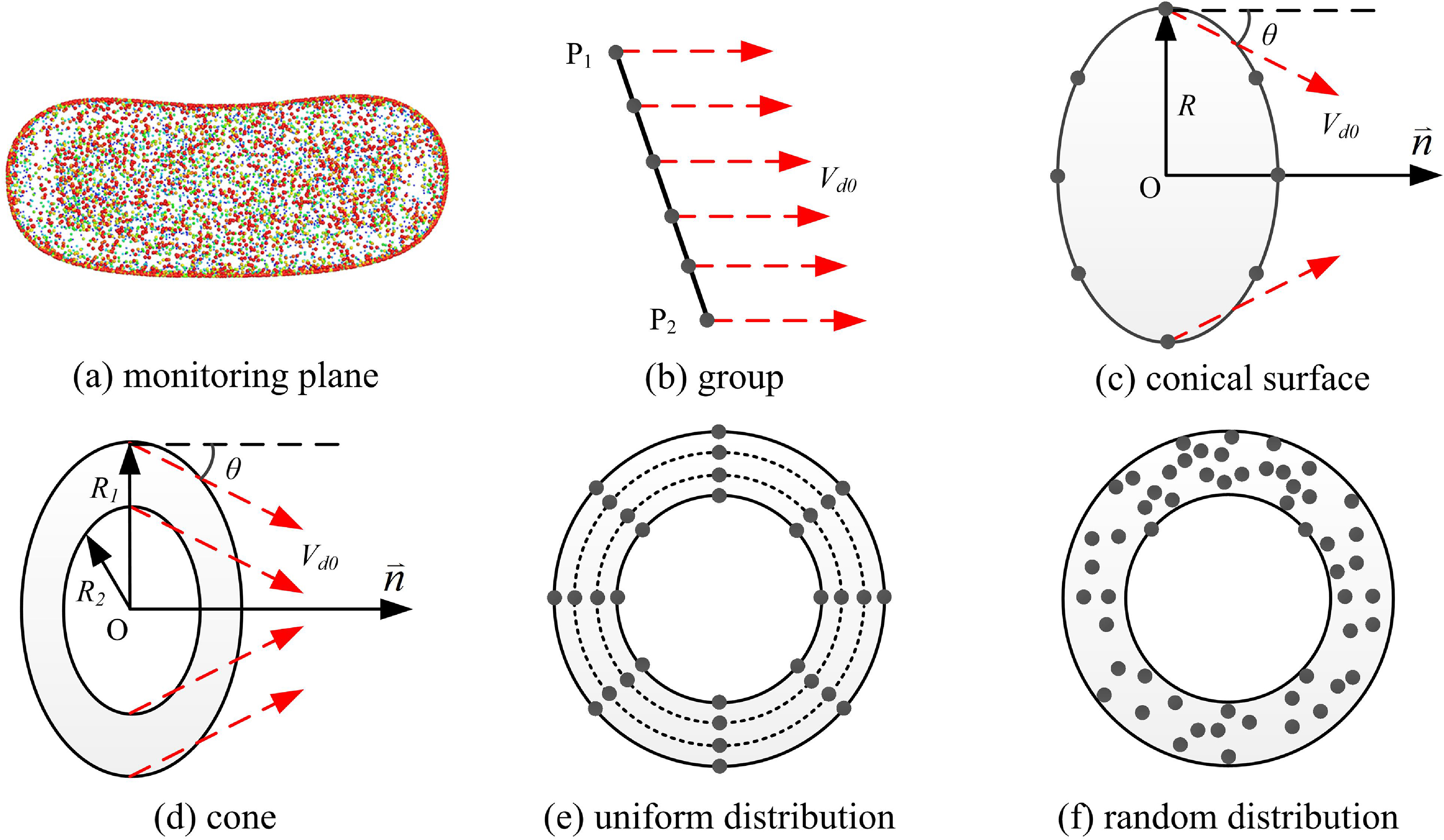
In DPMTrace, there are four particle injection types available to determine the initial distribution of particles, namely, monitoring plane, group, conical surface and cone, as shown in Fig. 11.
Four types of particle injection models available in the present particle tracking method: (a) monitoring plane, (b) group, (c) conical surface and (d) cone. Images (e) and (f) are respectively the uniform and random particle distribution models determining the initial particle position.

The monitoring surface injection type directly employs the planes that have been generated in the phase of meshing and yields a random distribution of the initial position of the particles at one monitoring surface (Fig. 11a). In the schematic of the group injection type (Fig. 11b),
 ${{\rm{P}}_{\rm{1}}}$
is the starting position,
 ${{\rm{P}}_{\rm{2}}}$
is the ending position and
 ${V_{d0}}$
is the initial injection velocity of particles. The particles are uniformly distributed between
 ${{\rm{P}}_{\rm{1}}}$
and
 ${{\rm{P}}_{\rm{2}}}$
at the starting moment. In the schematic of the conical surface injection type (Fig. 11c),
 $O$
is the origin of the cone.
 $\mathord{\buildrel{\lower3pt\hbox{$\scriptscriptstyle\rightharpoonup$}} \over n} $
is the axial direction of the conical surface.
 $R$
is the diameter of the conical surface.
 $\theta $
is the half-cone angle. The particles are uniformly distributed on the circumference of the bottom of the conical surface. In the schematic of the cone injection type (Fig. 11d),
 ${R_1}$
and
 ${R_2}$
are the outer and inner diameters of the cone, respectively. Besides, the particles can be initially distributed uniformly or randomly in the volume of the cone (Fig. 11e and f).
3.6 Particle tracking strategy
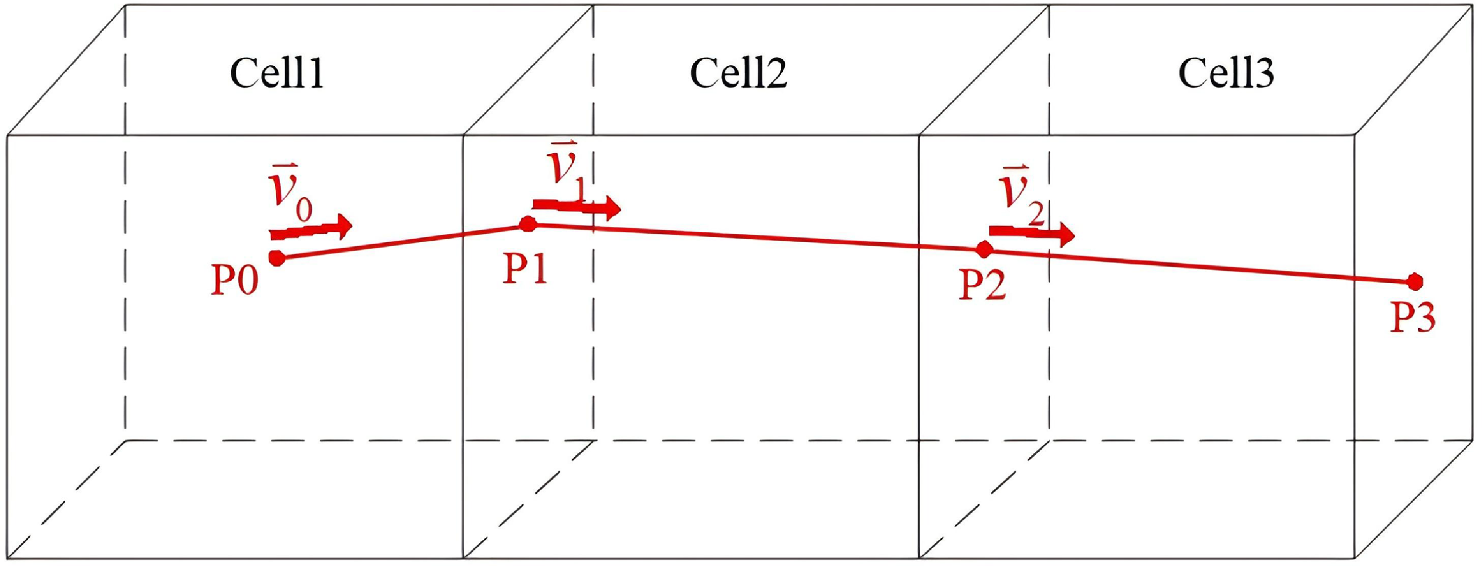
DPMTrace tracks the particle trajectory on a cell-by-cell level, as illustrated for a particle in Fig. 12. The tracking steps are described as follows:
-
(1) Assume that the particle with the initial velocity of
${\mathord{\buildrel{\lower3pt\hbox{$\scriptscriptstyle\rightharpoonup$}} \over v} _0}$
is initially located at the point
${\rm{P0}}$
in the body cell of Cell1. -
(2) Taking
${\rm{P0}}$
as the base point and the vector
${\mathord{\buildrel{\lower3pt\hbox{$\scriptscriptstyle\rightharpoonup$}} \over v} _0}$
as the direction, make a ray to intersect with the face element of Cell1 to get the point
${\rm{P1}}$
as the next position of the particle. The velocity of the particle at
${\rm{P1}}$
is:(10)where the acceleration
\begin{align}{\mathord{\buildrel{\lower3pt\hbox{$\scriptscriptstyle\rightharpoonup$}} \over v} _1} = {\mathord{\buildrel{\lower3pt\hbox{$\scriptscriptstyle\rightharpoonup$}} \over v} _0} + {a_1} \cdot {t_1}\end{align}
${a_1}$
is obtained from Equation (1) with the aerodynamic parameters taken from Cell1. Time
${t_1} = {{\rm{s}}_{\rm{0}}}/{v_0}$
, where
${{\rm{s}}_{\rm{0}}}$
is the distance between point
${\rm{P0}}$
and point
${\rm{P1}}$
.
-
(3) Similarly, all the subsequent positions,
${\rm{P2}}$
and
${\rm{P3}}$
, of the particle can be determined. Here, the connecting line of
${{P0\!-\!P1\!-\!P2\!-\!P3}}$
is formed and represents the trajectory of the particle.


Tracking method of the trajectory of a single particle.

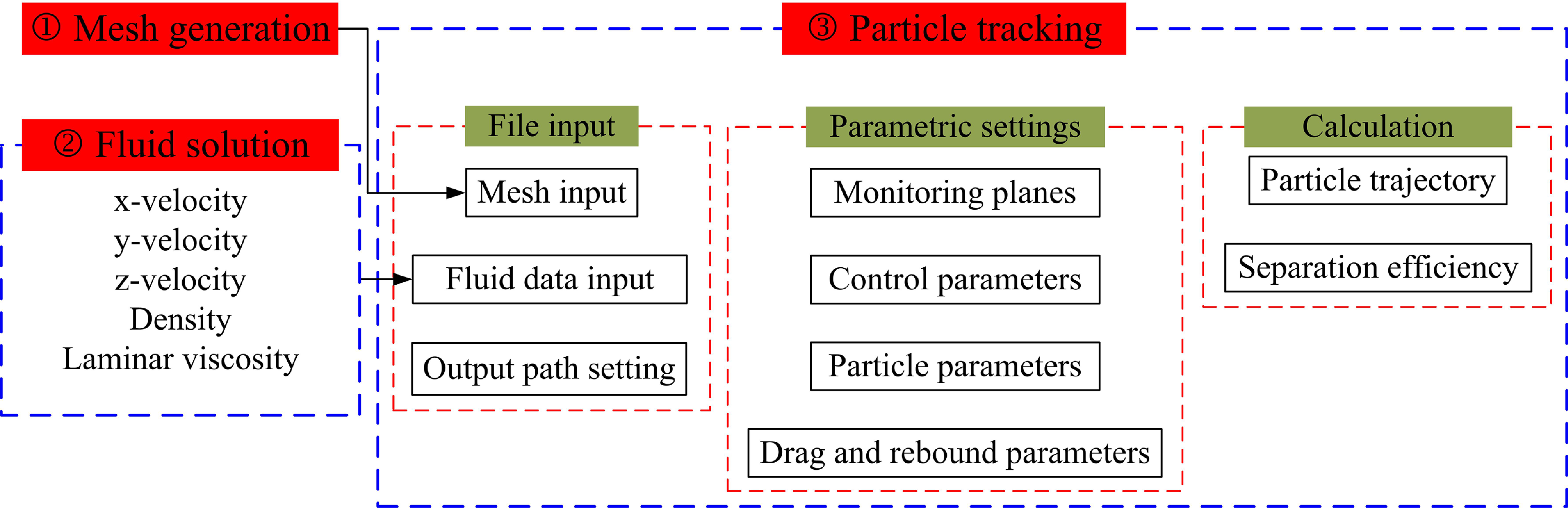
Flowchart of the current particle calculation method.

If the particle hits the boundaries of the cells during the movement, different treatments need to be taken, depending on the different types of boundaries: (1) if the particle hits an inlet or outlet of the computational domain, then it stops moving; (2) if the particle hits a monitoring plane, it continues to move and the particle information (position, velocity, etc.) is recorded when the particle crosses the monitoring plane; (3) if the particle hits a wall, the velocity and angle of the particle after rebound are calculated according to the wall rebound model introduced in Subsection 2.4.
3.7 Particle calculation flowchart
The in-house code ‘DPMTrace’ is purely a particle tracking code, namely the air flow field simulation and particle motion simulation are completely separated. The flowchart of particle calculation in this study is shown in Fig. 13. Generally, there are three major steps corresponding to the three calculation modules:
-
(1) Mesh generation. This is the first step to input the mesh generated by the commercial meshing software ANSYS ICEM [31]. Note that the current Eulerian–Lagrangian sediment transport method is based on fully structured meshes.
-
(2) Fluid solution. This is the second step to input the fluid solution data calculated by ANSYS Fluent [Reference Fluent29]. The necessary fluid solution data include the three components of the three-dimensional flow field, the density and laminar viscosity of the fluid.
-
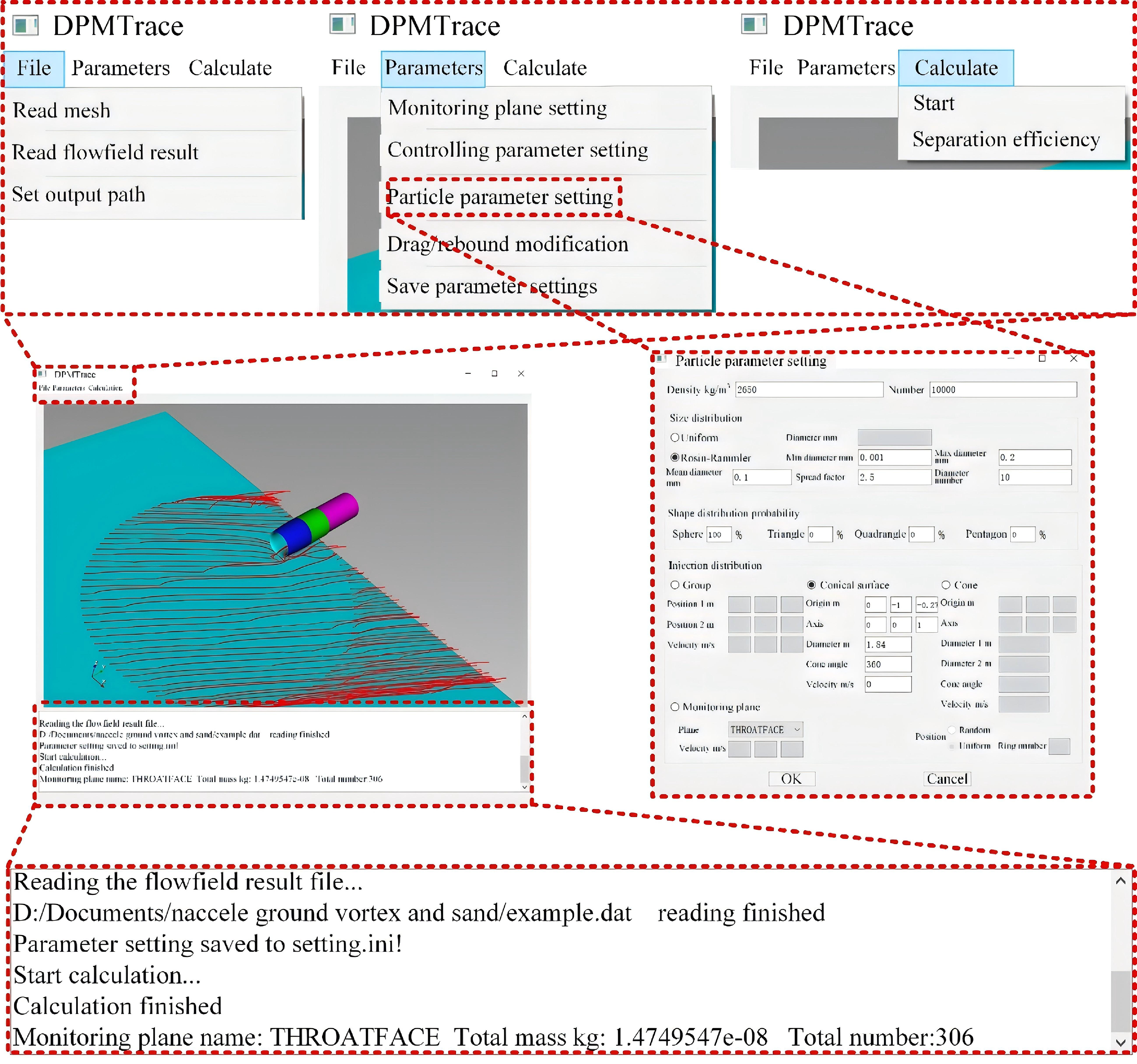
(3) Particle tracking. This is the core step to calculate the particle characteristics by the currently developed code DPMTrace. Herein, there are three sub-steps to follow sequentially, corresponding to the three modules in DPMTrace. The first module is file input, including the inputs of the mesh and fluid solution data, as well as the setting of the particle tracking results output path. Then it moves to the second module, i.e. parametric settings, including the settings of the monitoring planes, the control parameters, the particle parameters, as well as the drag and rebound parameters. The monitoring planes can be the boundary surfaces, like the outlet of the nacelle inlet or the interior planes that have been intentionally built for monitoring. The control parameters include the gravitational acceleration, the number of threads for parallel calculation and the interval of output of particle trajectory. The particle parameters include particle density, number of particles injected into the flow field, particle diameter distribution conforming to both the uniform and Rosin–Rammler (R–R) distributions, particle shape distribution probability and injection parameters. The drag and rebound parameters are included in the configuration data file under the installation folder. After setting all the above necessary parameters, it comes to the final module of calculation, i.e. calculation of the particles’ three-dimensional characteristics including the trajectory and concentration distribution, as well as the calculation of the separation efficiency for bifurcated flow channels, such as an inertial particle separator (IPS) [Reference Barone, Loth and Snyder35] for turboshaft engines and a turboprop engine inlet with bypass duct [Reference Zheng, Zhenlong, Huijun, Zhang and Kun36]. A local view of the DPMTrace interface is given in Fig. 14. It is noted that the developed DPMTrace software adopts a one-way coupled Eulerian–Lagrangian framework, in which the feedback effect of particles on the gas-phase flow field is neglected. This assumption is reasonable for the low particle-loading conditions considered in the present study, where particle-induced momentum exchange is negligible, and the gas-phase flow dominates particle transport. Therefore, the present method is mainly applicable to low- and moderate-concentration sand-ingestion conditions. Under extremely high particle-loading conditions, the momentum exchange between the particle and gas phases may become significant, and a two-way coupled framework would be more appropriate.
3.8 Particle tracking validation
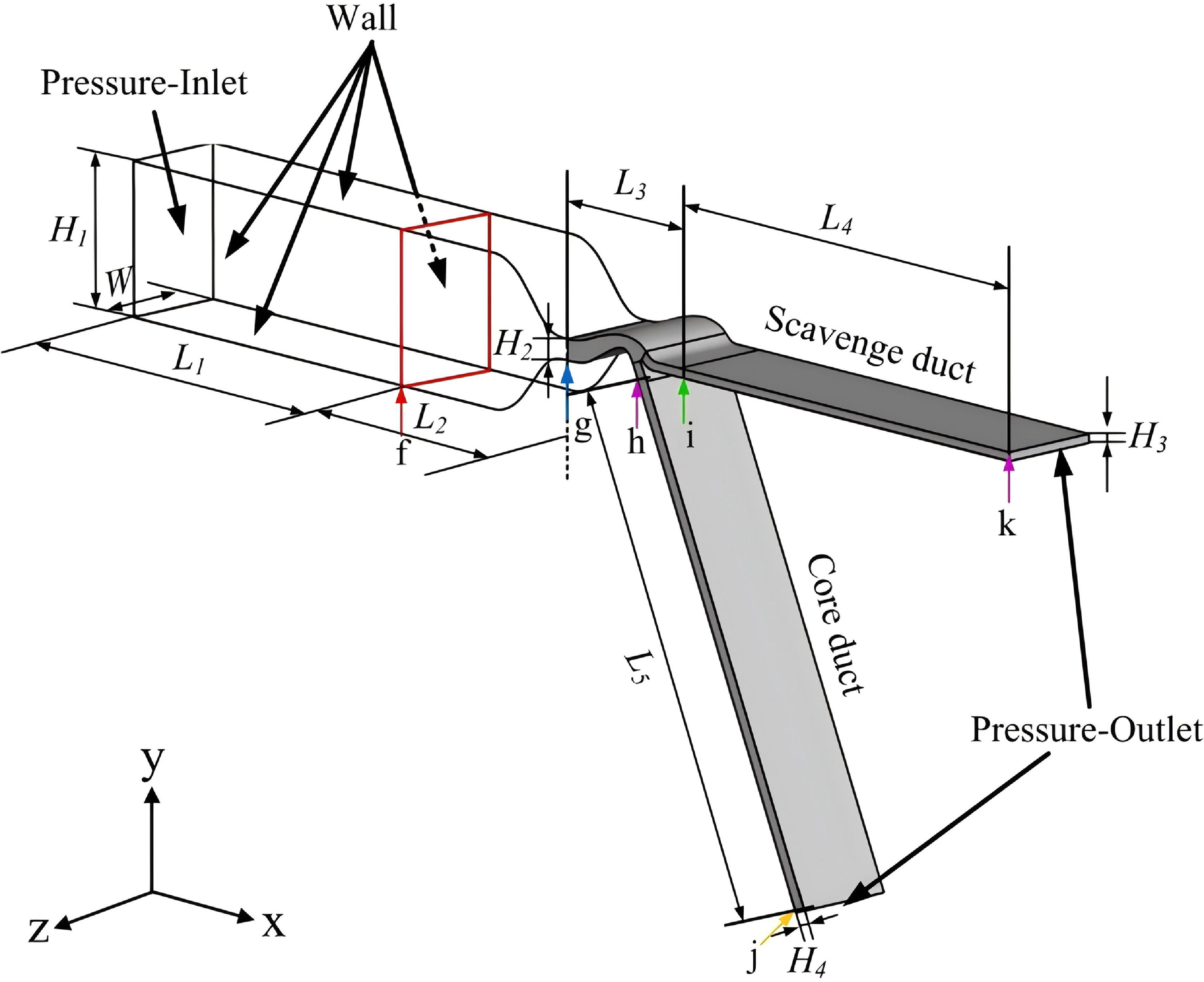
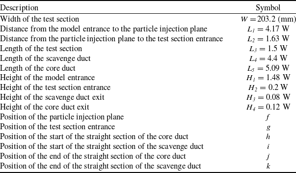
To validate the DPMTrace code, the IPS case studied comprehensively by Prof. Loth’s research group [Reference Barone, Loth and Snyder37] is chosen and calculated, of which the CFD model is shown in Fig. 15. The definitions and dimensions of the model are given in Table 5. The leftmost boundary plane is the entrance of the model, and there are two ducts, i.e. the core duct and scavenge duct, downstream of the IPS. The red cross-section is a virtual plane for generating the mesh of the particle injection plane. As for the boundary conditions, the entrance of the model was set as ‘Pressure-Inlet’, as well as both the exits of the core and scavenge ducts set as ‘Pressure-Outlet’, and all the rest of the boundary planes set as ‘No-Slip-Wall’.
Interface of the DPMTrace software.

Figure 14. Long description
A diagram of the DPMTrace software interface. The interface includes several tabs and windows for setting parameters and running simulations. Panel A shows the main interface with tabs for File, Parameters, and Calculate. The File tab includes options to read mesh, read flowfield result, and set output path. The Parameters tab includes options for monitoring plane setting, controlling parameter setting, particle parameter setting, drag rebound modification, and saving parameter settings. The Calculate tab includes options to start the calculation and check separation efficiency. Panel B shows the particle parameter setting window, which includes fields for density, number, size distribution, shape distribution probability, injection distribution, and monitoring plane settings. Panel C shows a simulation of particle flow with a 3D model and particle trajectories. The simulation includes labels for various dimensions and parameters such as height, length, diameter, and velocity. The diagram also includes text indicating the progress of reading the flowfield result file, saving parameter settings, starting and finishing calculations, and monitoring plane information.
Illustration of the CFD model of Loth’s IPS.

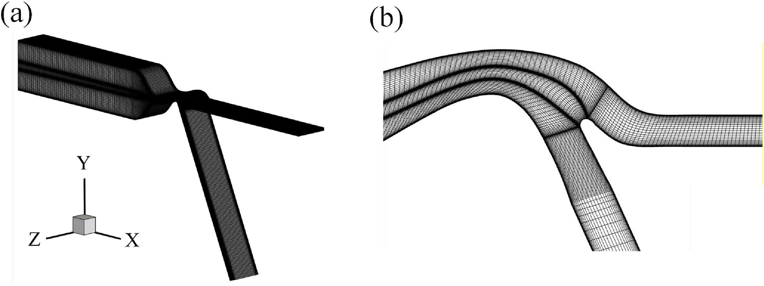
A fully structured mesh was generated to discretise the computational domain of the IPS model, as shown in Fig. 16. It has a total of 2,262,429 nodes and 2,373,448 elements. The height of the cell attached to the walls was set to 0.02 mm, yielding the maximum value of about 12 for the wall y
+. The steady compressible RANS equation was solved by the pressure-based solver in the commercial package ANSYS Fluent 2019 [Reference Fluent29] to obtain the air flow field of the IPS. The ST
 $k - \omega $
model [Reference Menter30] was chosen to simulate the turbulence of the air flow field. The spatial discretisation schemes were set the same as at the nacelle inlet, as described in Subsection 2.2. For the sand particle simulation, the properties of particles were set to match the experimental condition [Reference Barone, Loth and Snyder35].
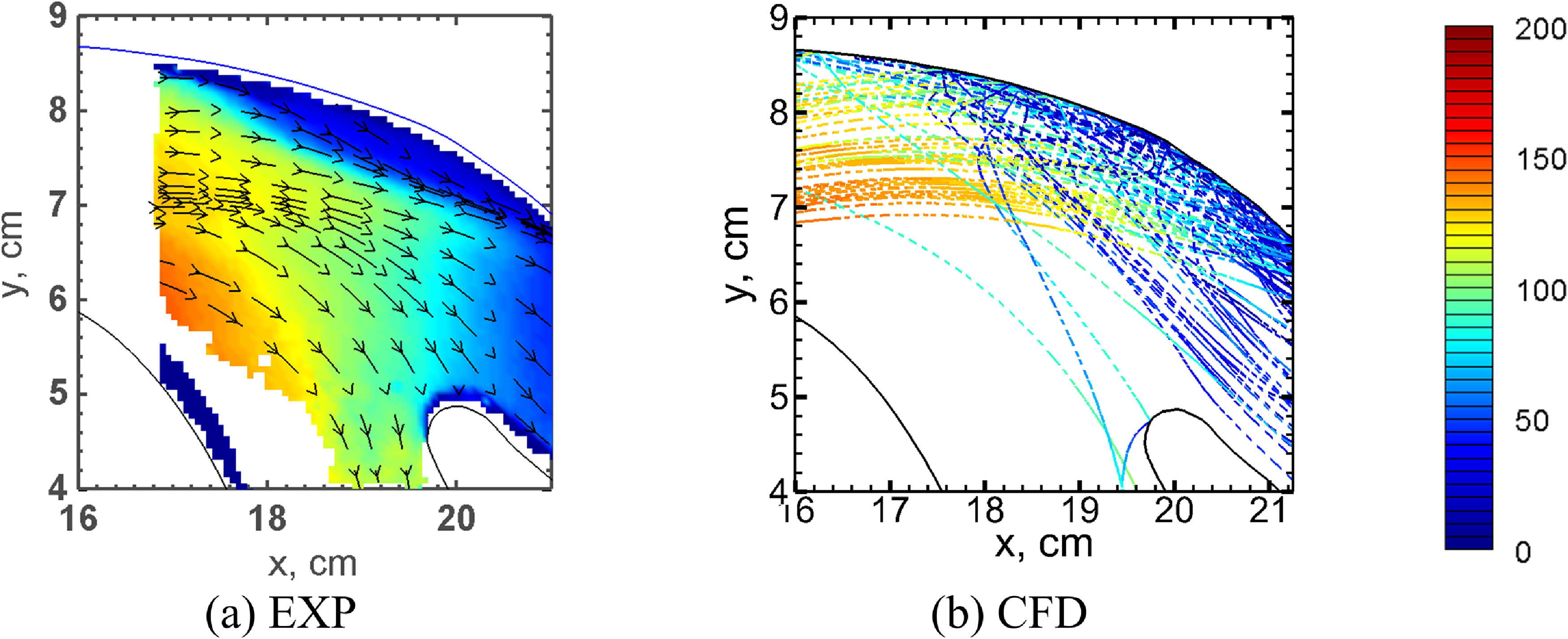
Figure 17 shows qualitative comparisons of the particle velocity fields of the IPS between Loth’s experimental measurements [Reference Barone, Loth and Snyder38] and our numerical results. Both the magnitude and direction of the fluid and particle velocities calculated by the current method are in good agreement with the referenced experimental results. To further quantitatively validate the DPMTrace code, the results of the particle separation efficiency
 $\eta $
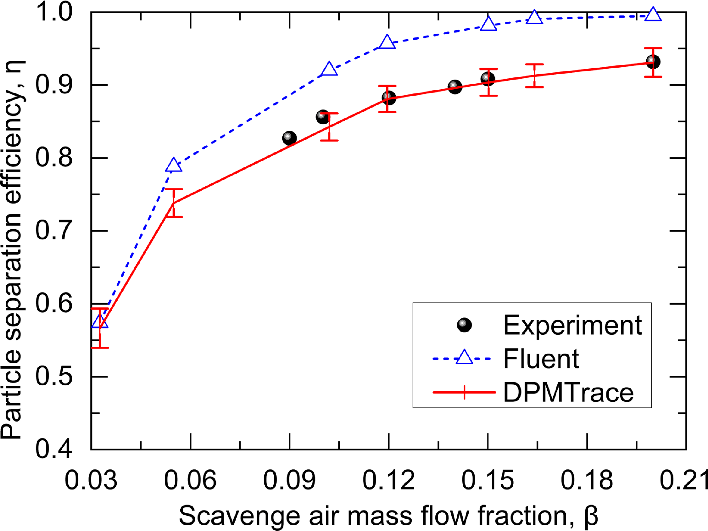
of the IPS were calculated with both the Discrete Phase Model DPM in ANSYS Fluent [Reference Fluent29] and the currently developed DPMTrace code shown in Fig. 18, together with Prof. Loth’s experimental measurements [Reference Barone, Loth and Snyder35]. Although the trend of the results calculated by Fluent is generally consistent with that of the experimental measurements, the magnitude is overestimated at all the simulation points, with a maximum of about 11.7%. In contrast, both the magnitude and trend of the results calculated by DPMTrace assume a fairly good agreement with the experimental measurements. Overall, it can be concluded that the currently developed DPMTrace scheme has a good performance in particle dynamics predictions.
4.0 Results and discussion
4.1 Pure ground vortex flow regimes
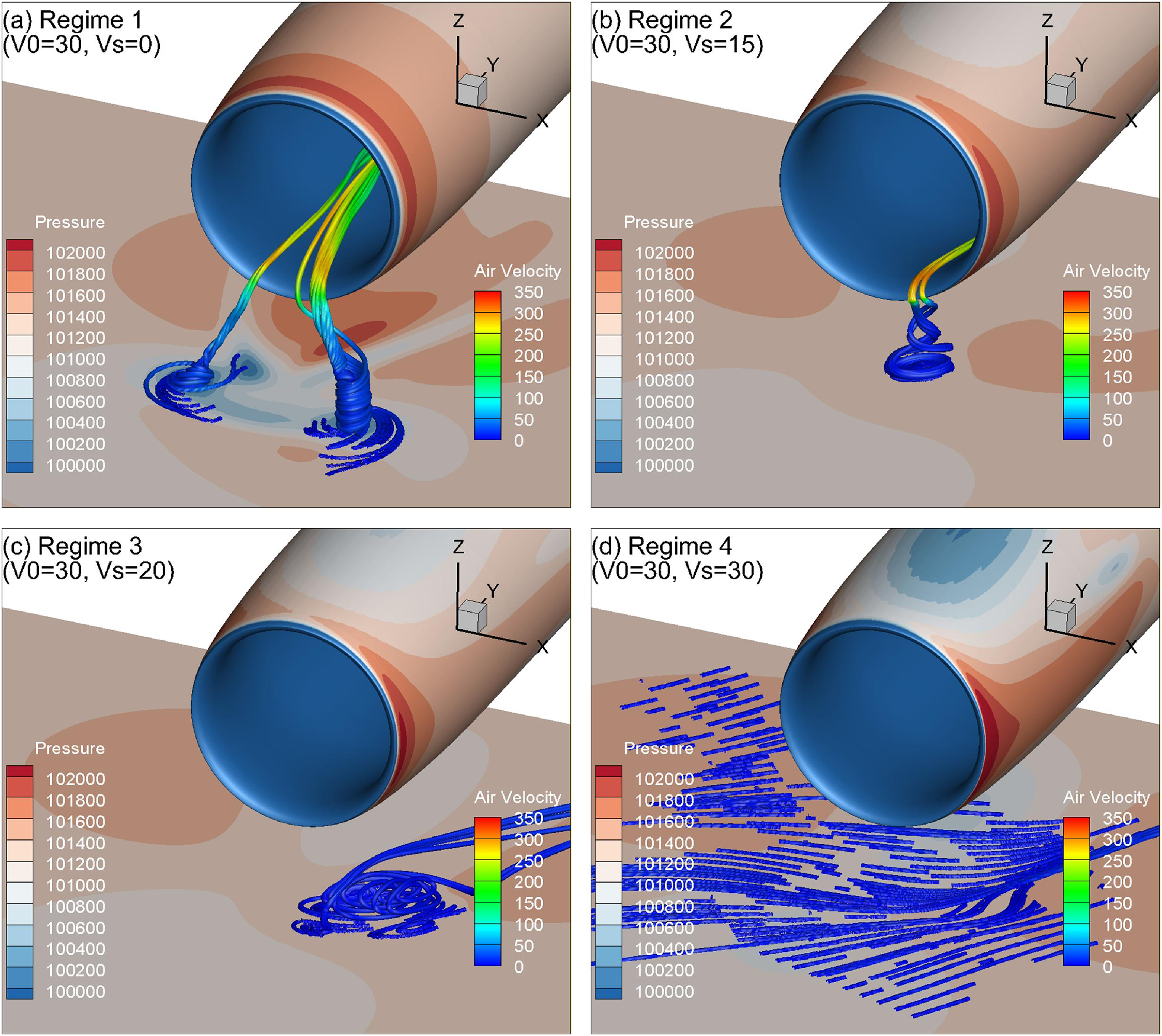
The ground vortex characteristics in the pure air flow field are the basis for the subsequent particle calculations, thus should be investigated first. The inlet capture area has been used by various scholars as a function describing the existence of the ground vortex [Reference De Siervi12, Reference Liu, Greitzer and Tan14]. Figure 19 presents the typical flow regimes regarding the ground vortex existence, including two vortices or a single vortex ingested into the inlet, a vortex formed on the ground but not ingested and no vortex. Regime 1 occurs at relatively lower side-wind speeds where the freestream airflow is separated into two main streams, resulting in two low-pressure areas on the ground and finally two ground vortices. In Regime 2, one side of the nacelle becomes the upwind side, depending on the direction of the side wind. Therefore, only one stagnation point is formed on the ground to finally evolve into a single ground vortex at the lee side. Further increasing side-wind speeds to Regime 3 causes the ground vortex directly to be blown away with no vortex ingested into the inlet. In Regime 4, no ground vortex is formed due to the extremely low mass flow ratio.
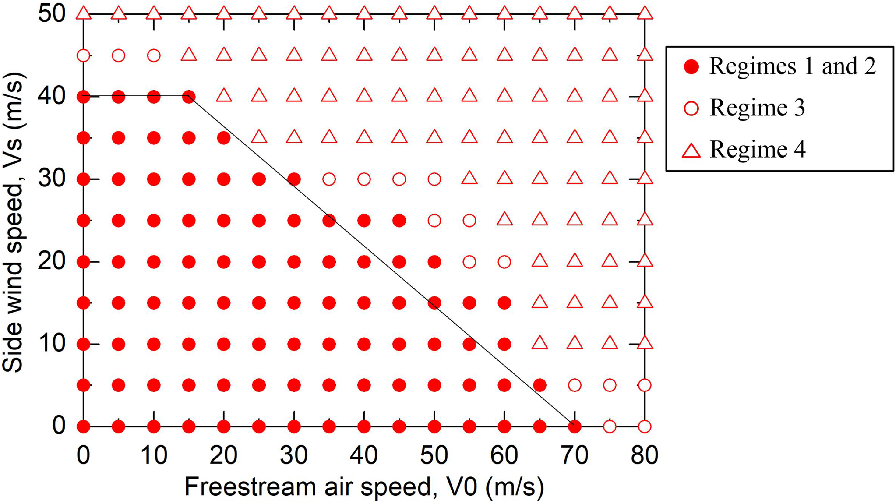
Figure 20 shows a map of the simulated ground vortex characteristics in terms of freestream air speed and side-wind speed. The solid circles incorporate ground vortices occurring within the above-mentioned Regimes 1 and 2, where they are all ingested into the inlet. The hollow symbols represent flow patterns within Regimes 3 and 4, where the ground vortex developed is not ingested into the inlet or is even absent. Generally, there is a clear ingestion boundary for the ground vortex existence, although there are several points located outside the boundary. The map also reflects that the ground vortex ingestion characteristics are more sensitive to side-wind speed than freestream air speed. Therefore, side wind is a critical factor that has attracted more and more attentions of ground vortex researchers recently.
4.2 Sand ingestion rate vs freestream air speed
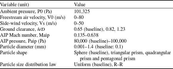
In this study, the characteristics of sand ingestion coupled with the ground vortex are comprehensively studied through several parametric perspectives. The variables and their value ranges are tabulated in Table 6. It should be noted that the selected parameter ranges include both representative engineering conditions and extended conditions used to investigate the underlying particle-ingestion mechanisms of nacelle inlets. Side-wind velocities below 20 m/s correspond to the majority of practical operating environments encountered by aircraft near the ground. Regarding the ground-clearance parameter, the cases of h/D = 0.82 and 1.23 represent practical engine-to-ground clearances commonly encountered by nacelle inlets during aircraft ground operations. In addition, the AIP Mach number of nacelle inlets is typically greater than 0.4 under practical operating conditions. The investigated freestream air velocity range of 0–80 m/s covers typical aircraft ground-operation phases, including taxiing, takeoff and landing. Parameter values beyond these representative engineering ranges are included to reveal the particle-ingestion mechanisms and evaluate the sensitivity of ingestion behaviour to key parameters, rather than to represent specific engine operating conditions. The following subsections extend a detailed description and discussion of the sand particle ingestion characteristics and mechanisms behind these aspects. In each run of the following particle calculations, a total number of 10,000 particles were injected from the ground surface with zero velocity. The ingestion rate, β, is defined as the mass ratio of particles ingested into the inlet to the total particles injected into the computational domain. It is worth noting that the baseline parameters had been taken into calculation unless particularly pointed out.
Definitions and dimensions of the model geometry of Loth’s IPS

Table 5. Long description
A table with two columns and sixteen rows. The first column is labeled Description and the second column is labeled Symbol. The table lists various dimensions and positions related to a model geometry. Row 1: Width of the test section, W = 203.2 millimeters. Row 2: Distance from the model entrance to the particle injection plane, L1 = 4.17 W. Row 3: Distance from the particle injection plane to the test section entrance, L2 = 1.63 W. Row 4: Length of the test section, L3 = 1.5 W. Row 5: Length of the scavenge duct, L4 = 4.4 W. Row 6: Length of the core duct, L5 = 5.09 W. Row 7: Height of the model entrance, H1 = 1.48 W. Row 8: Height of the test section entrance, H2 = 0.2 W. Row 9: Height of the scavenge duct exit, H3 = 0.08 W. Row 10: Height of the core duct exit, H4 = 0.12 W. Row 11: Position of the particle injection plane, f. Row 12: Position of the test section entrance, g. Row 13: Position of the start of the straight section of the core duct, h. Row 14: Position of the start of the straight section of the scavenge duct, i. Row 15: Position of the end of the straight section of the core duct, j. Row 16: Position of the end of the straight section of the scavenge duct, k.
Mesh of the validated IPS: (a) global view of the computational domain and (b) close view of the test section.

Comparisons of the fluid and particle velocity fields of the IPS between (a) experiment and (b) CFD.

Comparison of the particle separation efficiency between the experimental measurements, CFD results by Fluent and the current in-house DPMTrace code.

Regimes of the ground vortex at ground clearance of h/D = 0.82: (a) Regime 1 with two ground vortices, (b) Regime 2 with a single ground vortex, (c) Regime 3 with significant ground vorticity but no ground vortex ingestion and (d) Regime 4 with no significant ground vorticity.

Ingestion boundary of ground vortex at fixed Paip = 80,000 Pa and h/D = 0.65.

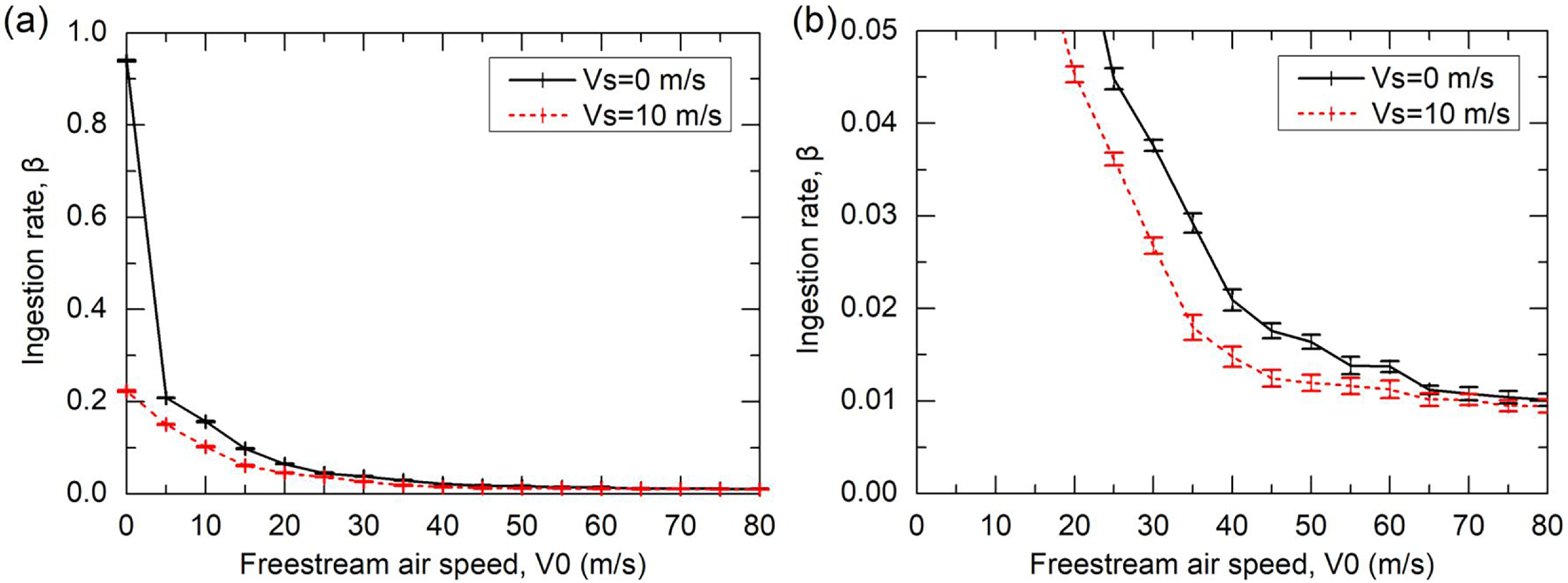
The particle ingestion characteristics coupling with the ground vortex shall also be affected by the influencing factors of the ground vortex, besides the properties of the particle itself. Figure 21 shows the variation of particle ingestion rate with freestream air speed at two given side-wind speeds. It is seen that the ingestion rate decreases with increasing freestream air speed (i.e. equivalently decreasing ground vortex strength) at fixed side-wind speeds till converging within Regimes 3 and 4. The unique condition of both zero freestream air and side-wind speeds produces the maximum ingestion rate of around 94%, because there is always a strong ground vortex due to the infinite stream tube area in this circumstance. The ingestion rate finally converges to about 1% rather than absolutely zero, although there has been no ground vortex formed or ingested. This implies that a ground vortex is not the sole factor dominating the ingestion of particles into the inlet.
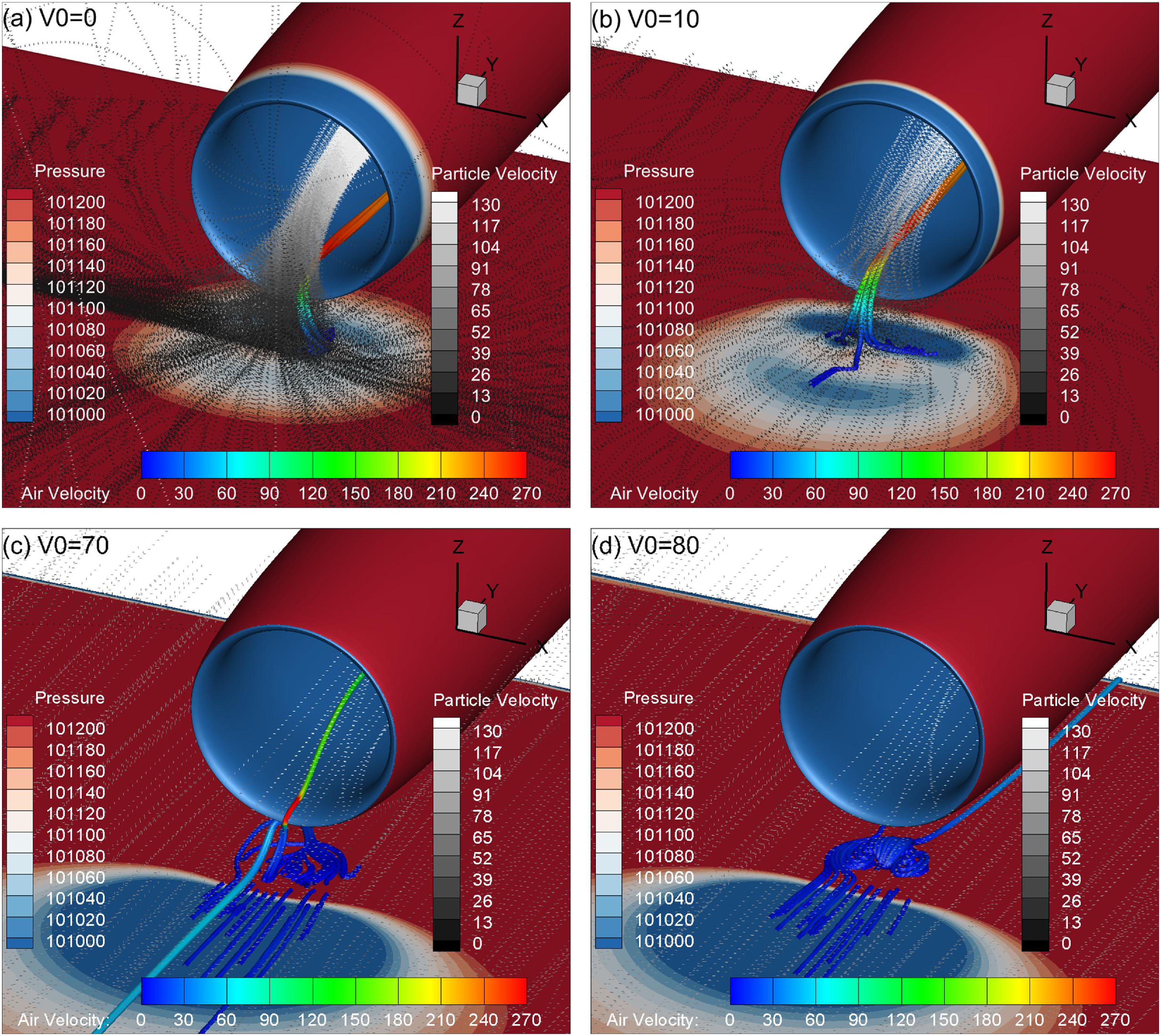
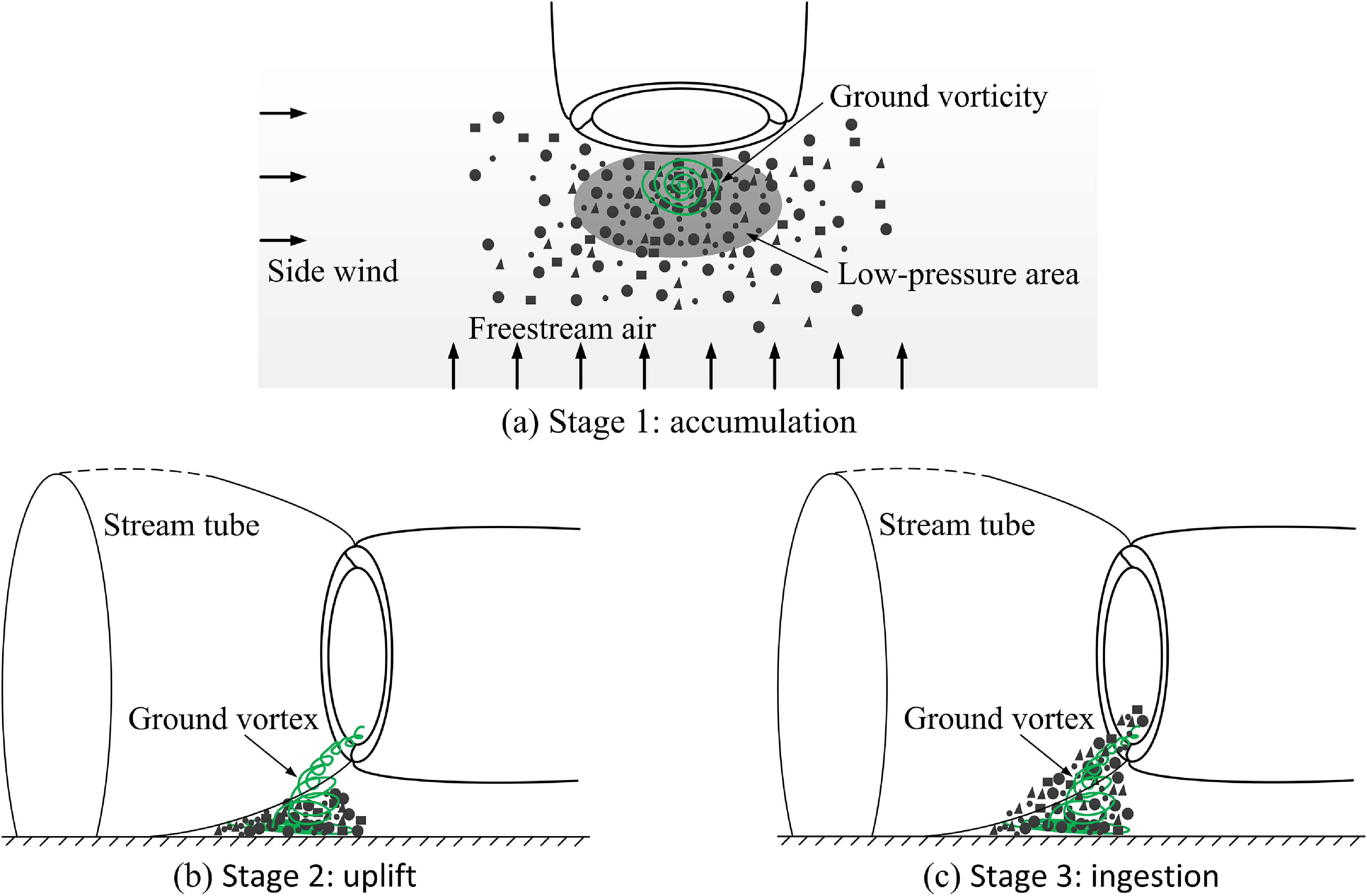
Figure 22 compares the distributions of particle ingestion trajectory and airflow pressure between various freestream air speeds. For the convenience of comparing both the particle and ground vortex trajectories, the ground vortex trajectory calculated at the same condition is superposed in each subfigure. Note that, for clarity, the number of particle ingestion trajectories has been reduced by 10 times, and one dotted curve herein represents one complete particle trajectory. Several findings can be obtained from Fig. 22. First, the strength of the ground vortex becomes weaker as freestream air speed decreases and finally is diverted out of the inlet at the highest freestream air speed. Second, the ingested particles seem not to follow the ingestion trajectory of the ground vortex, revealing that the ingestion of the ground vortex is not the straightforward cause of particle ingestion. Third, when the ground vortex is strong, the particles seem to first gather to the low-pressure region on the ground surface from all around of the far field, and then are uplifted and accelerate to enter the inlet (Fig. 22a and b). Fourth, even if the ground vortex becomes weaker or even absent, there are still a handful of particles being ingested as there is still significant flow vorticity at the ground. This ground vorticity seems to have a tight relation with the ingestion of particles, as will be discussed further.
4.3 Sand ingestion rate vs side-wind speed
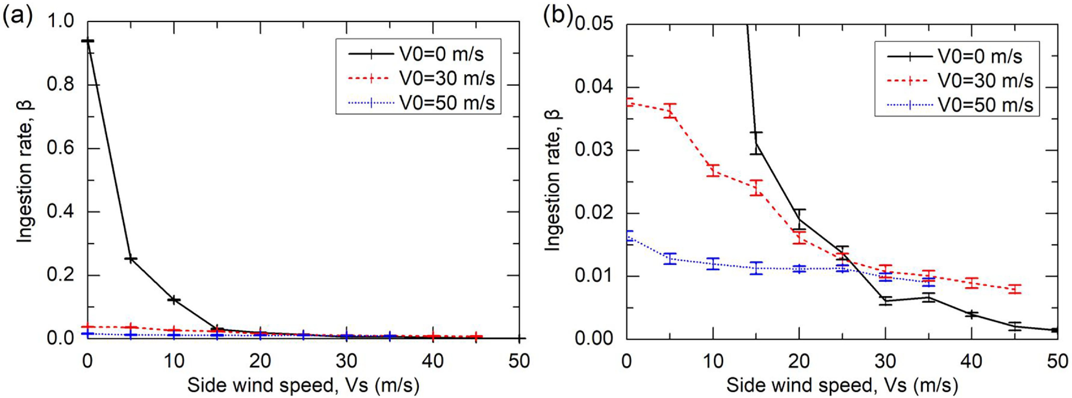
Figure 23 presents the variation of particle ingestion rate with side-wind speed at three given freestream air speeds, which exhibits the same trend as that with freestream air speed. Still and all, some differences can be found between the results under the influences of side-wind and freestream air. First, the particle ingestion rate decreases more rapidly with the increasing side-wind speed than with the increasing freestream air speed. Second, the ingestion rate almost converges to zero when the aircraft is static (V0 = 0 m/s), while it reaches a converged value of 1% under the freestream air conditions (Fig. 21b). However, as the freestream air is involved (V0 = 30 and 50 m/s), the convergence value of the ingestion rate is increased to about 1% again. The above results manifest that side wind has a more dominating influence on the particle ingestion results at relatively low side-wind speeds, while freestream air does at higher side-wind speeds.
Value ranges of the variables involved in this study

Table 6. Long description
A table with two columns and eleven rows. The first column lists variable names and their units, and the second column lists their corresponding value ranges. The variables include ambient pressure, freestream air velocity, side-wind velocity, ground clearance, AIP Mach number, AIP pressure, particle diameter, particle shape, and particle size distribution law. Each variable is listed with its unit in parentheses and the value range provided in the adjacent cell.
Note: h is the engine axis height off the ground, D is the internal diameter of the AIP of the inlet.
Particle ingestion rate vs freestream air speed. Subfigure (b) is an amplified view of (a).

Distributions of the particle trajectory (dotted curves) and ground vortex trajectory (rod) at Vs = 0 m/s with (a) V0 = 0 m/s, (b) V0 = 10 m/s, (c) V0 = 70 m/s and (d) V0 = 80 m/s.

Particle ingestion rate vs side-wind speed for drop size of 0.1 mm. Subfigure (b) is an amplified view of (a).

Figure 23. Long description
Two line graphs depict the ingestion rate as a function of side wind speed for different freestream air velocities. Panel A: The line graph shows the ingestion rate on the vertical axis and the side wind speed in meters per second on the horizontal axis. Three different freestream air velocities are represented: 0 meters per second with a solid black line, 30 meters per second with a dashed red line, and 50 meters per second with a dotted blue line. The ingestion rate decreases sharply as the side wind speed increases from 0 to 10 meters per second and then levels off near zero for higher side wind speeds. Panel B: This line graph is an amplified view of Panel A, focusing on lower ingestion rates. The vertical axis ranges from 0 to 0.05, and the horizontal axis ranges from 0 to 50 meters per second. The same three freestream air velocities are represented with the same line styles and colors. The ingestion rate decreases more gradually compared to Panel A, with visible error bars indicating variability in the measurements.
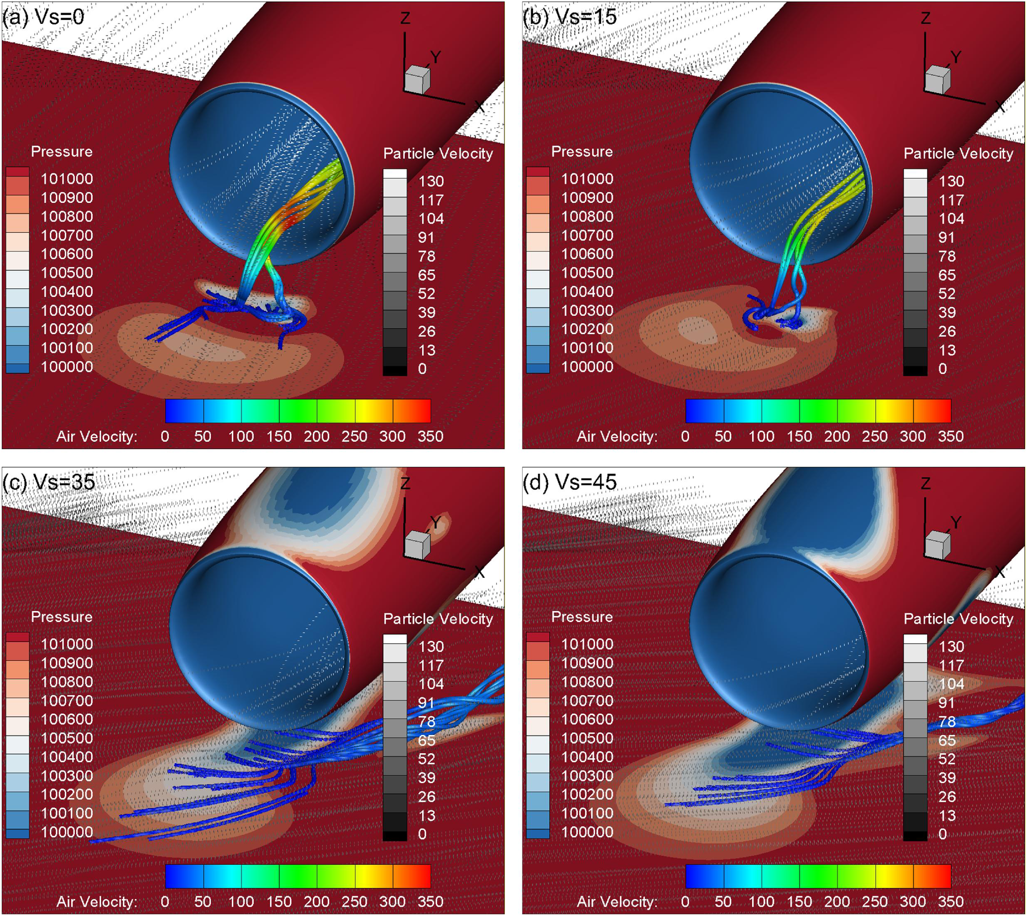
It can be seen from Fig. 24 that the particle ingestion trajectory corresponds well to the direction of side wind. Moreover, the number of ingested particles is reduced as side wind is increased. Because of the higher freestream air speed, the strength of the ground vortex is weaker, so particles are not able to gather from the periphery. Instead, they are entrained by the coupling action of the freestream air and side wind, and ingested into the inlet together with the stream tube. In particular, although there is no ground vortex ingested at side speeds of 35 and 45 m/s, there is still significant ground vorticity beneath the lip of the inlet, inducing a few particles to saltate off the ground [Reference Johnson, Leishman and Sydney39] and be ingested by the stream tube into the inlet.
Distributions of the particle trajectory (dotted curves) and ground vortex trajectory (rod) at V0 = 30 m/s with (a) Vs = 0 m/s, (b) Vs = 15 m/s, (c) Vs = 35 m/s and (d) Vs = 45 m/s.

4.4 Sand ingestion rate vs AIP Mach number
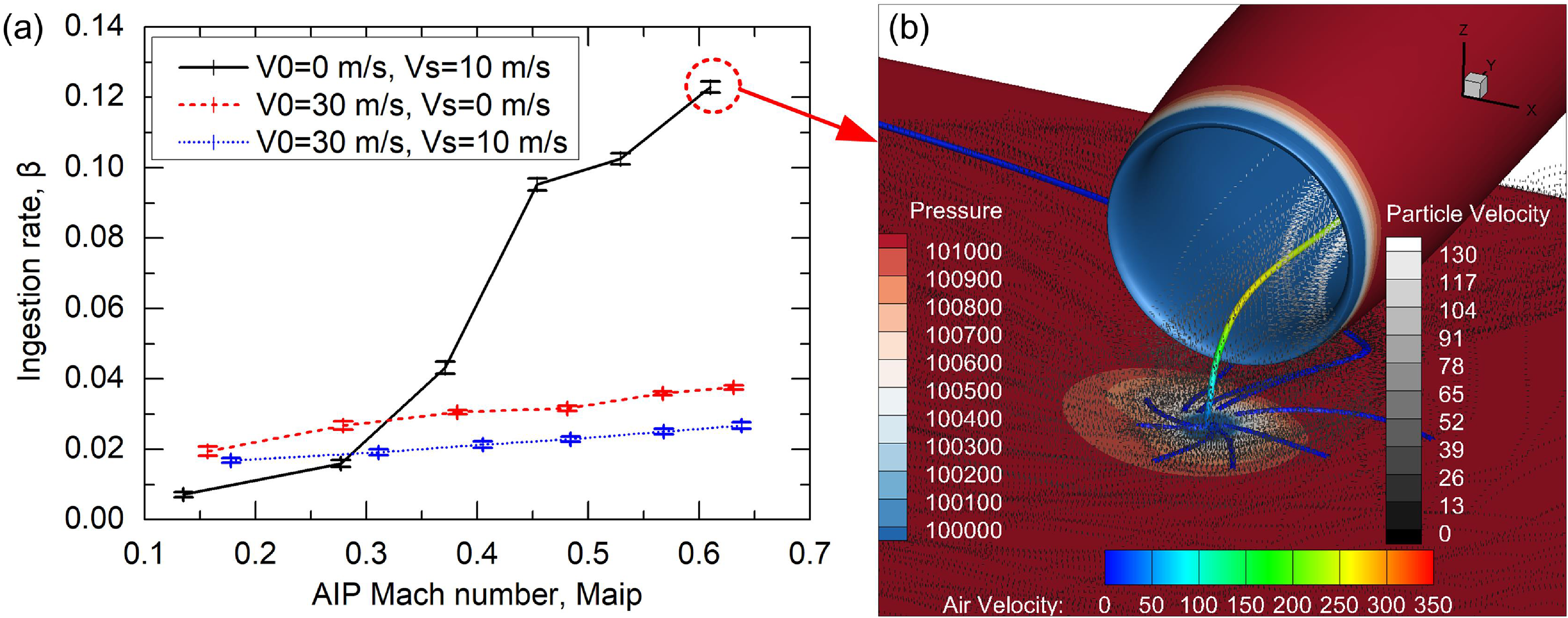
In addition to the aforementioned external flow conditions, the influence of internal flow conditions of the inlet also deserves attention. It can be seen from Fig. 25a that the particle ingestion rate increases monotonically with the Mach number of the AIP at the inlet. Taking the maximum value point as an example, the local low-pressure region at V0 = 0 m/s and Vs = 10 m/s (Fig. 25b) is much larger than that at V0 = 30 m/s and Vs = 10 m/s (Fig. 24a). Therefore, many more particles are gathered from the periphery to the low-pressure region and are ingested into the inlet along with the strong ground vortex. In addition, it can also be found that the low-pressure region plays a much more dominating role in determining the particle ingestion rate than the strength of the ground vortex.
(a) Particle ingestion rate vs AIP Mach number for drop size of 0.1 mm at h/D = 0.65, (b) distributions of the particle trajectory (dotted curves) and ground vortex trajectory (rod) at V0 = 0 m/s and Vs = 10 m/s and Maip = 0.61.

Figure 25. Long description
The image contains two panels labeled (a) and (b). Panel A: A line graph shows the ingestion rate (beta) on the vertical axis against the AIP Mach number (Maip) on the horizontal axis. The graph includes three data series represented by different line styles: solid black, dashed red, and dotted blue. Each series corresponds to different initial velocities (V0) and side-wind velocities (Vs). The solid black line represents V0=0 meters per second and Vs=10 meters per second, the dashed red line represents V0=30 meters per second and Vs=0 meters per second, and the dotted blue line represents V0=30 meters per second and Vs=10 meters per second. The ingestion rate increases with the AIP Mach number for all series, with the solid black line showing the steepest increase. Panel B: A 3D visualization shows the distributions of particle trajectories (dotted curves) and ground vortex trajectory (rod) at V0=0 meters per second and Vs=10 meters per second and Maip=0.61. The visualization includes color scales for pressure, particle velocity, and air velocity. The pressure scale ranges from 100100 to 101100, the particle velocity scale ranges from 0 to 130, and the air velocity scale ranges from 0 to 350. The particle trajectories and ground vortex are depicted within a 3D space with axes labeled X, Y, and Z.
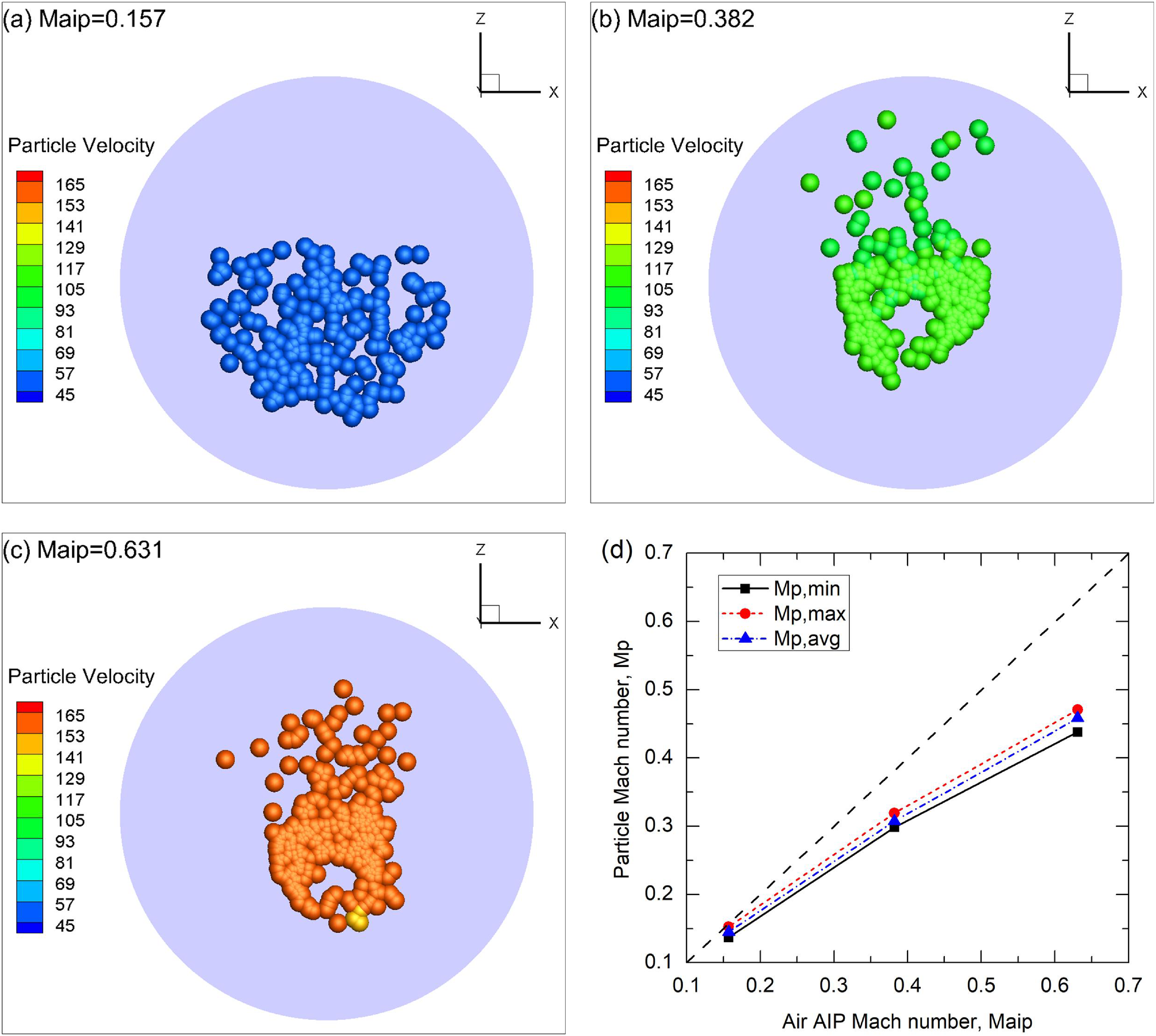
The distribution characteristics of particles at the AIP are presented in Fig. 26. Note that the particle size has been amplified by 200 times for clarity in all of this paper. Due to the interaction between the two phases under different internal flow conditions as well as the consideration of the probability of the particle rebound on the walls of the inlet, the distribution morphology assumes significant differences between the various Mach number of AIP (Maip), especially at relatively low Maip. Besides, although all the particles are initially injected from the ground surface with zero speed, they are all accelerated by the high-speed internal flow inside the inlet. It is this increased high speed that causes accumulative erosions of compressor blades by ingested particles [Reference Hill and Franklin9]. However, the acceleration of the ingested particles is not equal and is obviously dependent on Maip. Figure 26d plots the minimum, maximum and average values of the ingested particles at the three values of Maip. It is visible that there is always a velocity difference between the particles and the airflow, which becomes larger as the internal flow speed increases.
Particle distribution characteristics at the AIP position of the inlet for different AIP Mach numbers at V0 = 30 m/s and Vs = 0 m/s: (a) Maip = 0.157, (b) Maip = 0.382 and (c) Maip = 0.631. (d) shows the relationships between the particle and air Mach numbers. The particle size is uniformly 0.1 mm.

4.5 Sand ingestion rate vs ground clearance
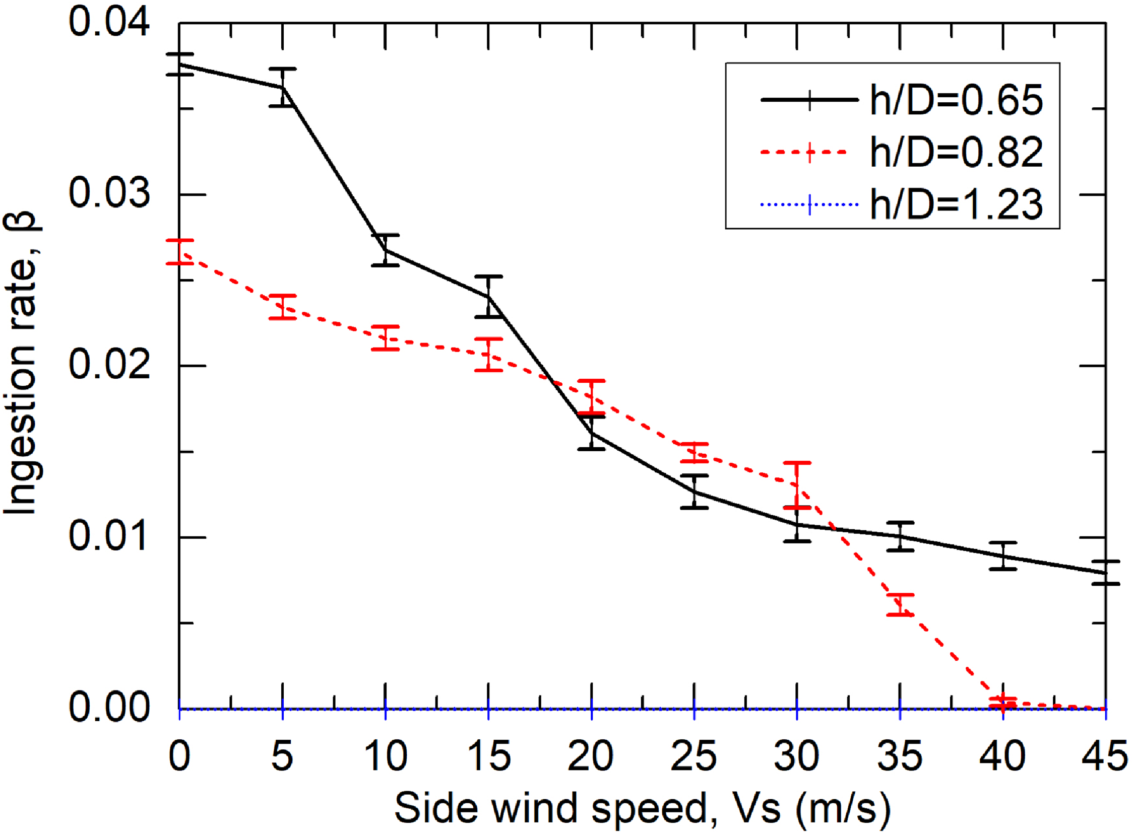
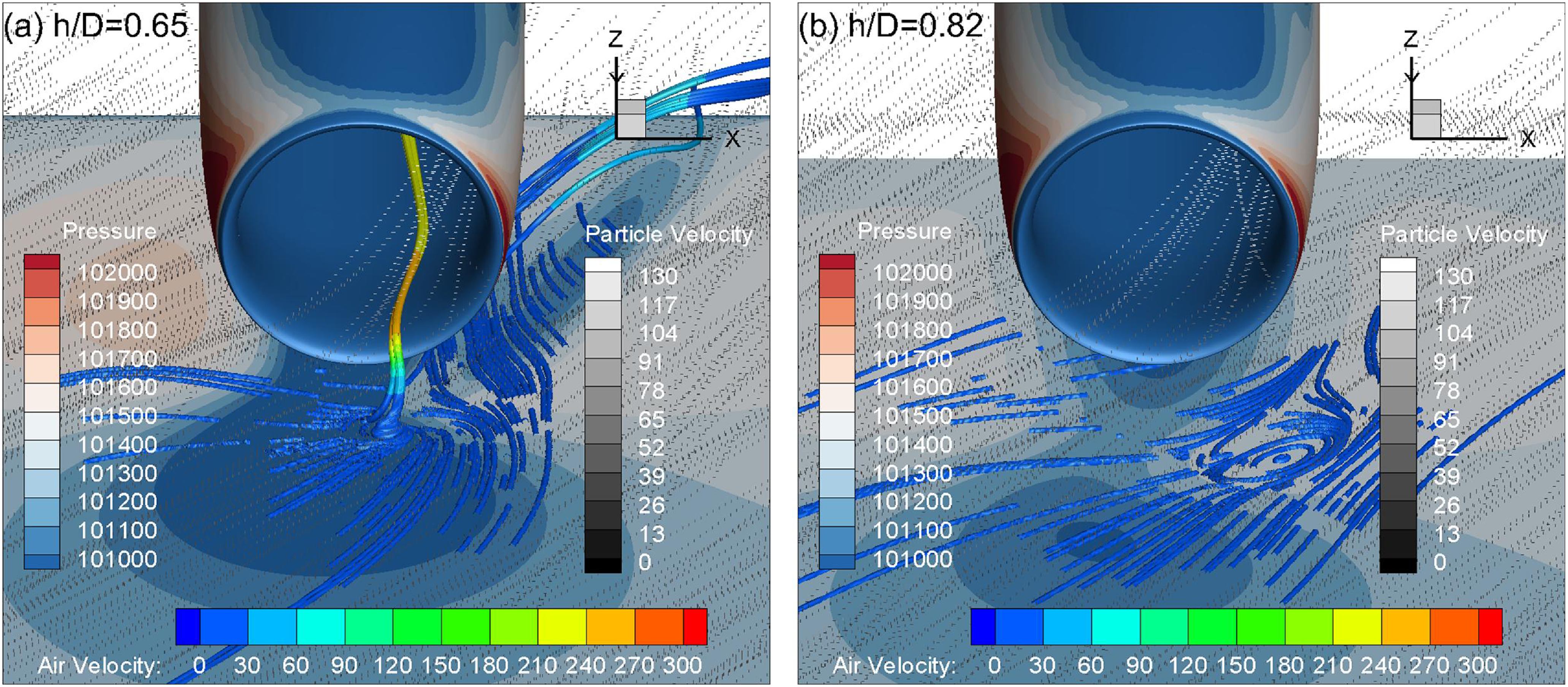
In addition to the related flow conditions, the ground clearance, i.e. the distance between the nacelle inlet and the ground surface, is also a factor of concern. It is shown in Fig. 27 that the ingestion rate is generally lower at a larger ground clearance. As the ground clearance increases to 1.23, no particle is ingested into the inlet at the side-wind speeds of interest. It is noted that there is an intersection between the side-wind speeds of 15 and 35 m/s, where the ingestion rate at h/D = 0.65 is unconventionally lower than that at h/D = 0.82. As shown in Fig. 28b, a larger ground vorticity area is generated at h/D = 0.82, although it does not develop into a fully ingested ground vortex. This enlarged vortical structure alters the particle transport paths and weakens the direct downstream convection induced by the side wind. More particles remain within the inlet capture region and are subsequently entrained into the inlet. By contrast, at h/D = 0.65, particles are transported more directly downstream by the side wind, leading to a lower ingestion rate under these conditions. Therefore, despite the larger ground clearance, the ingestion rate at h/D = 0.82 becomes slightly higher than that at h/D = 0.65 over the side-wind speed range of approximately 15–35 m/s.
Particle ingestion rate vs ground clearance for drop size of 0.1 mm at V0 = 30 m/s.

Distributions of the particle trajectory (dotted curves) and ground vortex trajectory (rod) for two different ground clearances at V0 = 30 m/s and Vs = 25 m/s: (a) h/D = 0.65 and (b) h/D = 0.82.

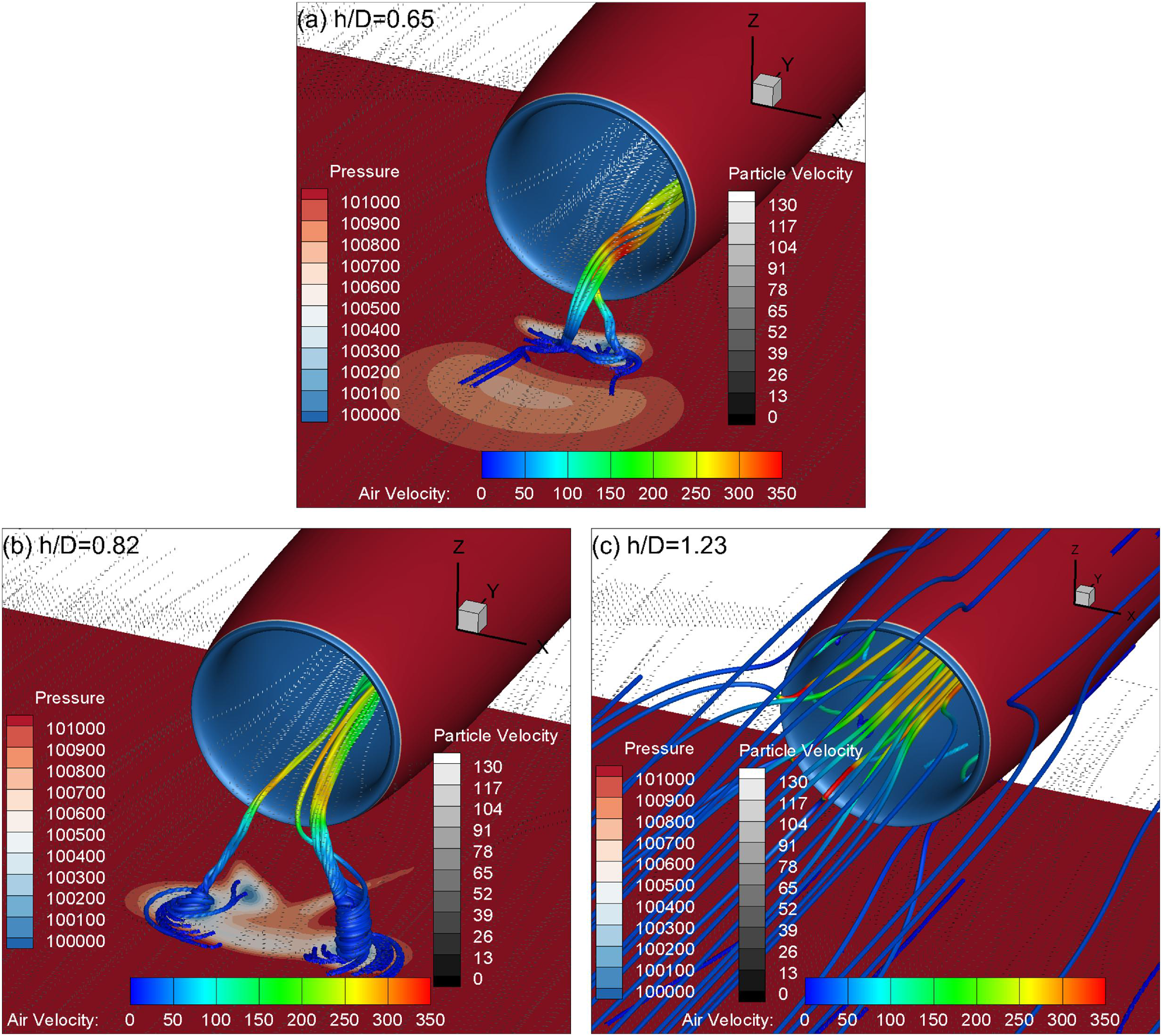
Figure 29 shows the influence of ground clearance on the particle ingestion rates. Two streams of ground vortices are clearly seen at the lowest ground clearance. As h/D increases to 0.82, the distance between the cores of the two ground vortices is increased while the ingestion speeds of both vortices are decreased. The increased distance weakens the interaction between both vortices at h/D = 0.82; therefore, fewer particles are entrained by the ground vortices to be ingested into the inlet. As h/D further increases to 1.23, there is no flow vorticity at the ground, so that no particle can be lifted off the ground. Instead, all the particles are transported with the freestream air near the ground surface to downstream and outside of the inlet.
Distributions of the particle trajectory (dotted curves) and ground vortex trajectory (rod) for the three ground clearances at V0 = 30 m/s and Vs = 0 m/s: (a) h/D = 0.65, (b) h/D = 0.82 and (c) h/D = 1.23.

Figure 29. Long description
The image contains three separate diagrams labeled (a), (b), and (c), each showing particle trajectories and ground vortex trajectories for different ground clearances. The diagrams are used to compare the effects of varying ground clearances on particle and vortex behavior. Panel A: This diagram shows the particle trajectory and ground vortex trajectory for a ground clearance ratio (h/D) of 0.65. The diagram includes a color-coded legend indicating pressure, particle velocity, and air velocity. The pressure is represented by a color scale ranging from 100100 to 101000, particle velocity by a grayscale ranging from 0 to 130, and air velocity by a color scale ranging from 0 to 350. The particle trajectories are depicted as dotted curves, and the ground vortex trajectory is shown as a rod. The axes are labeled with Z and Y directions. Panel B: This diagram shows the particle trajectory and ground vortex trajectory for a ground clearance ratio (h/D) of 0.82. Similar to Panel A, it includes a color-coded legend for pressure, particle velocity, and air velocity. The pressure scale ranges from 100100 to 101000, particle velocity from 0 to 130, and air velocity from 0 to 350. The particle trajectories are shown as dotted curves, and the ground vortex trajectory is depicted as a rod. The axes are labeled with Z and Y directions. Panel C: This diagram shows the particle trajectory and ground vortex trajectory for a ground clearance ratio (h/D) of 1.23. It also includes a color-coded legend for pressure, particle velocity, and air velocity. The pressure scale ranges from 100100 to 101000, particle velocity from 0 to 130, and air velocity from 0 to 350. The particle trajectories are depicted as dotted curves, and the ground vortex trajectory is shown as a rod. The axes are labeled with Z and Y directions.
4.6 Sand ingestion rate vs particle properties
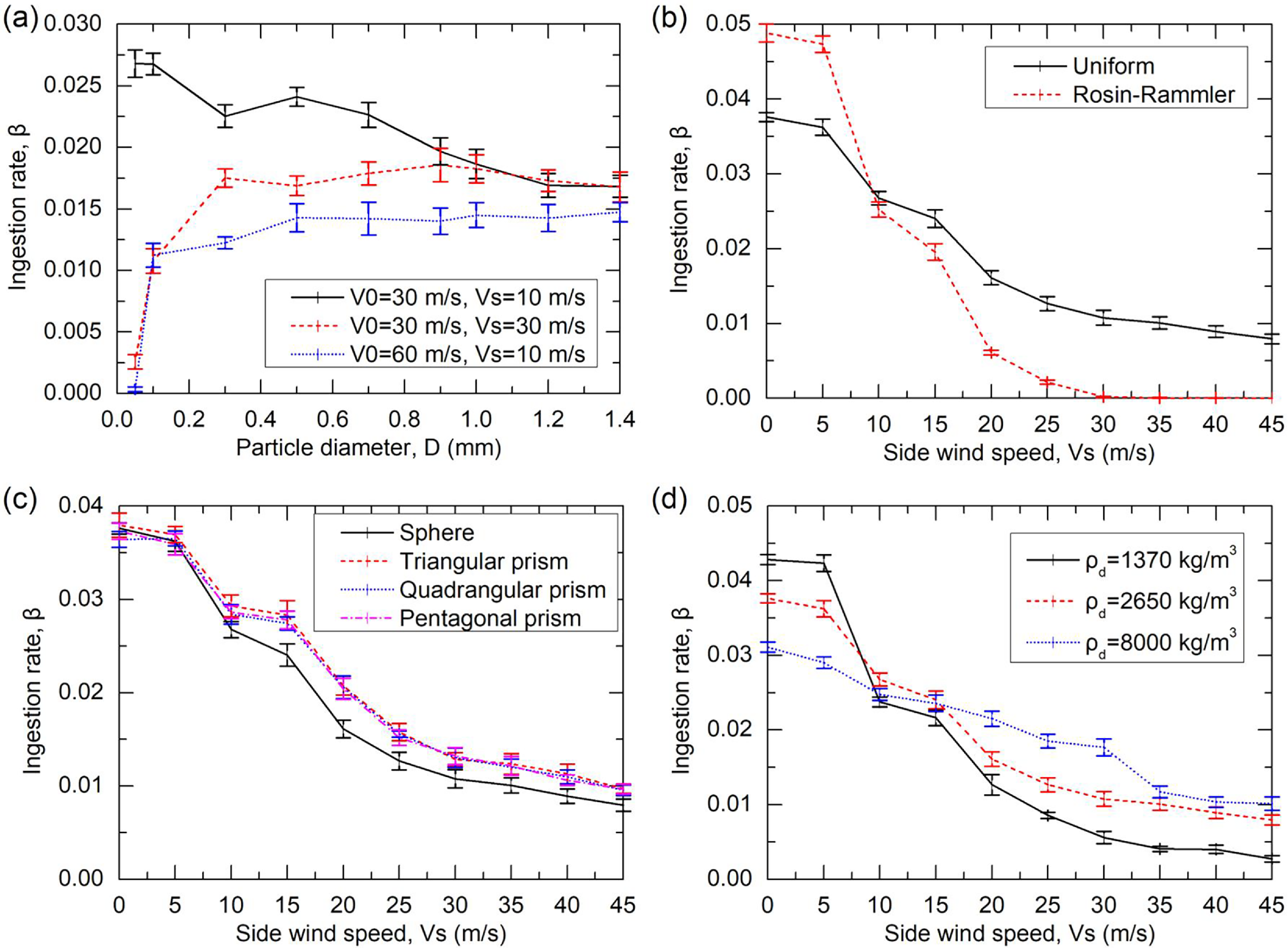
The particle ingestion characteristics are no doubt related to the physical properties of the particles. Figure 30 sequentially shows the influences of particle size, size distribution law, shape and density on the particle ingestion rate. As for the particle size influence, it can be seen from Fig. 30a that the ingestion rate finally converges as the particle size increases to 1.2 mm, because of the balance between the gravitational force and aerodynamic force for such larger particles.
Particle ingestion rate vs (a) particle size, (b) size distribution, (c) shape, and (d) density at V0=30 m/s

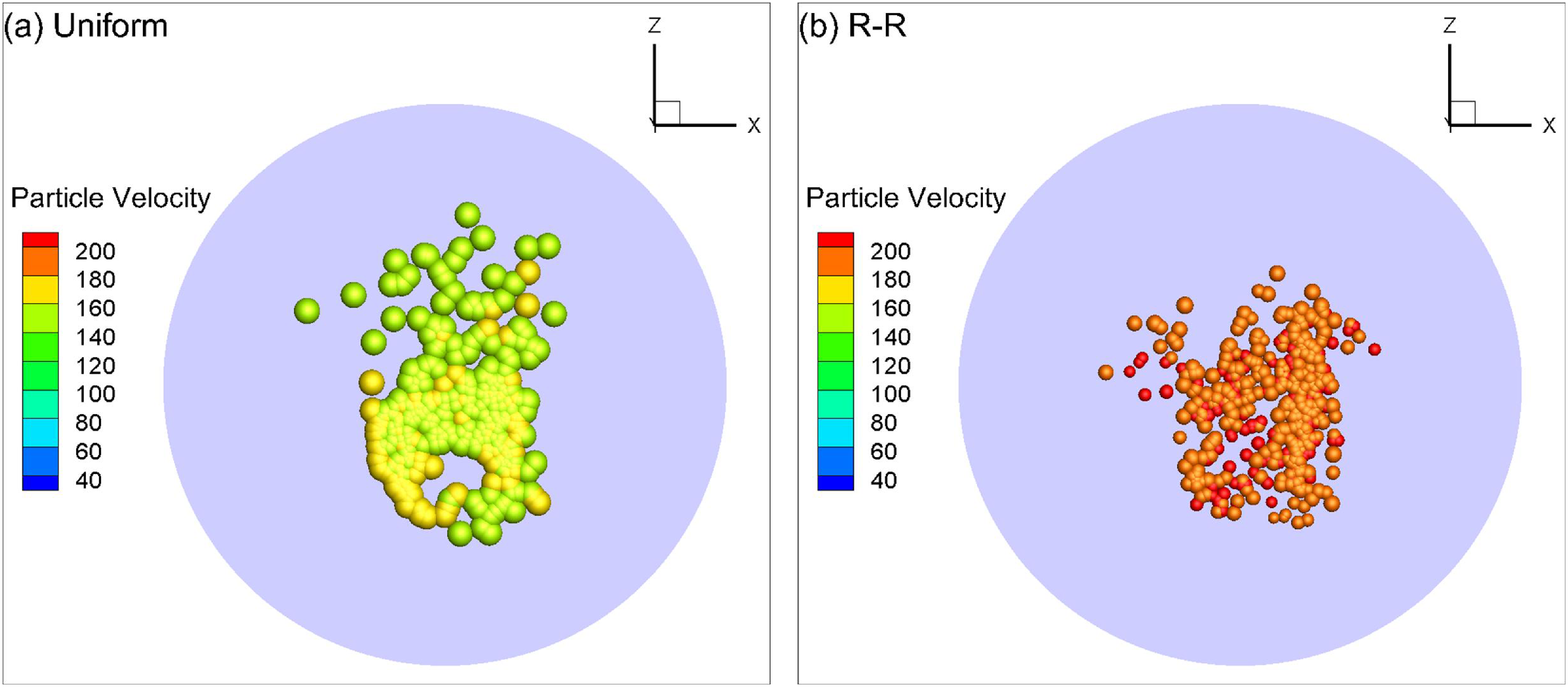
Particle distribution at the AIP of the inlet under both size distribution laws at V0 = 30 m/s and Vs = 0 m/s: (a) uniform size distribution and (b) R–R size distribution. The (mean) particle size is 0.1 mm.

It is found from Fig. 30b that the ingestion rate of particles under the R–R size distribution law is larger at side-wind speeds lower than 10 m/s while it becomes smaller beyond 10 m/s. Note that the average size of the R–R distributed particles is equal to that of uniform particles of 0.1 mm. It is known from Fig. 31 that the diameters of the ingested particles under the R–R size distribution law are much smaller than those of uniform-sized particles. Thus, at lower external flow speeds (lower side-wind speeds or freestream air speeds) when the ground vorticity is relatively stronger, the smaller R–R distributed particles can better be ingested into the inlet in a manner similar to that shown in Fig. 22a. However, at larger external flow speeds when the ground vorticity is weak or even absent, the smaller R–R distributed particles are more prone to flow outside of the inlet in a manner similar to that shown in Fig. 24d. It is also known from Fig. 31 that the R–R distributed particles reach higher speeds at the AIP due to their better streamability with a lighter weight.
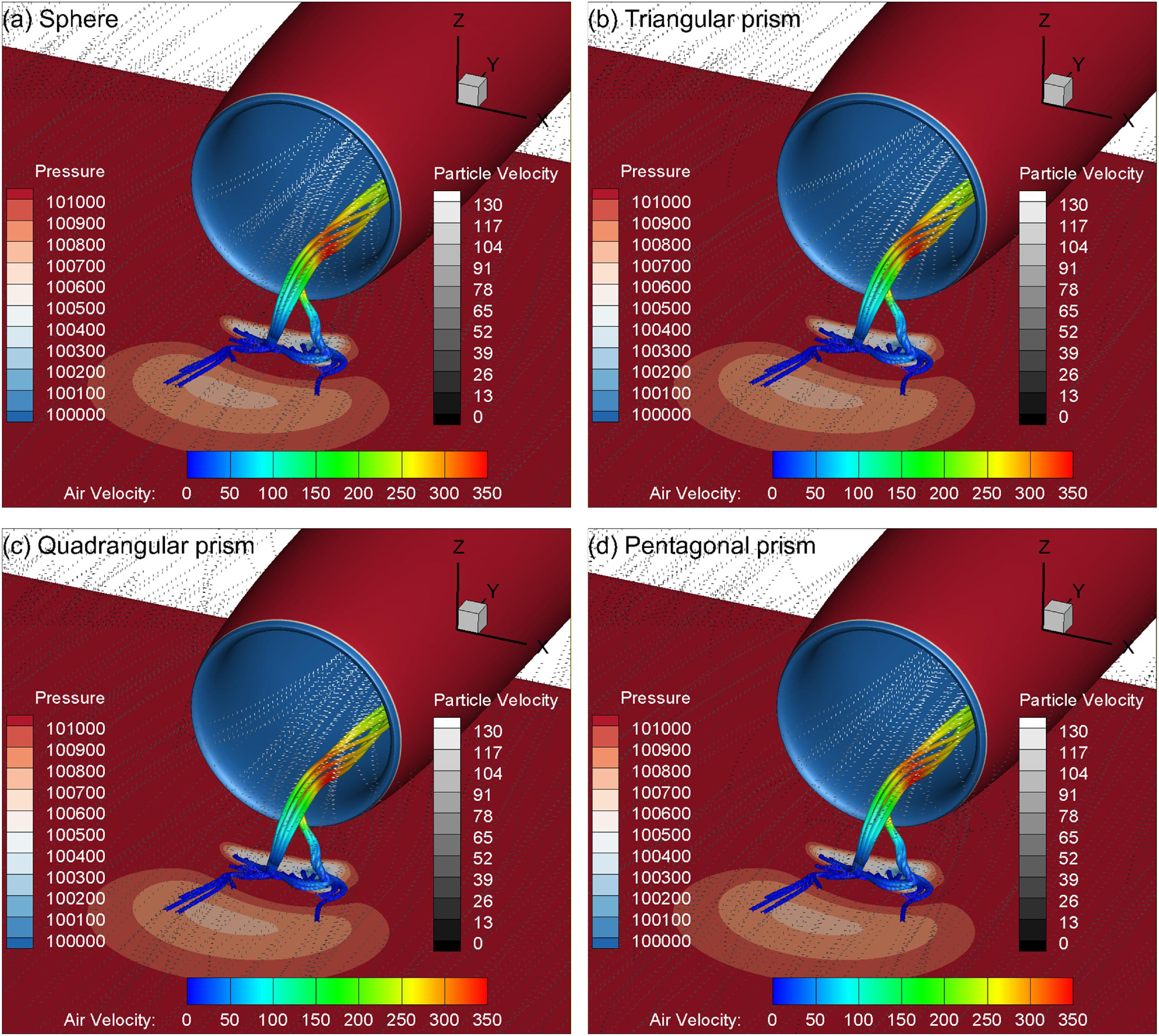
Distributions of the particle trajectory (dotted curves) and ground vortex trajectory (rod) for different particle shapes at V0 = 30 m/s, Vs = 0 m/s and h/D = 0.65: (a) sphere, (b) triangular prism, (c) quadrangular prism and (d) pentagonal prism.

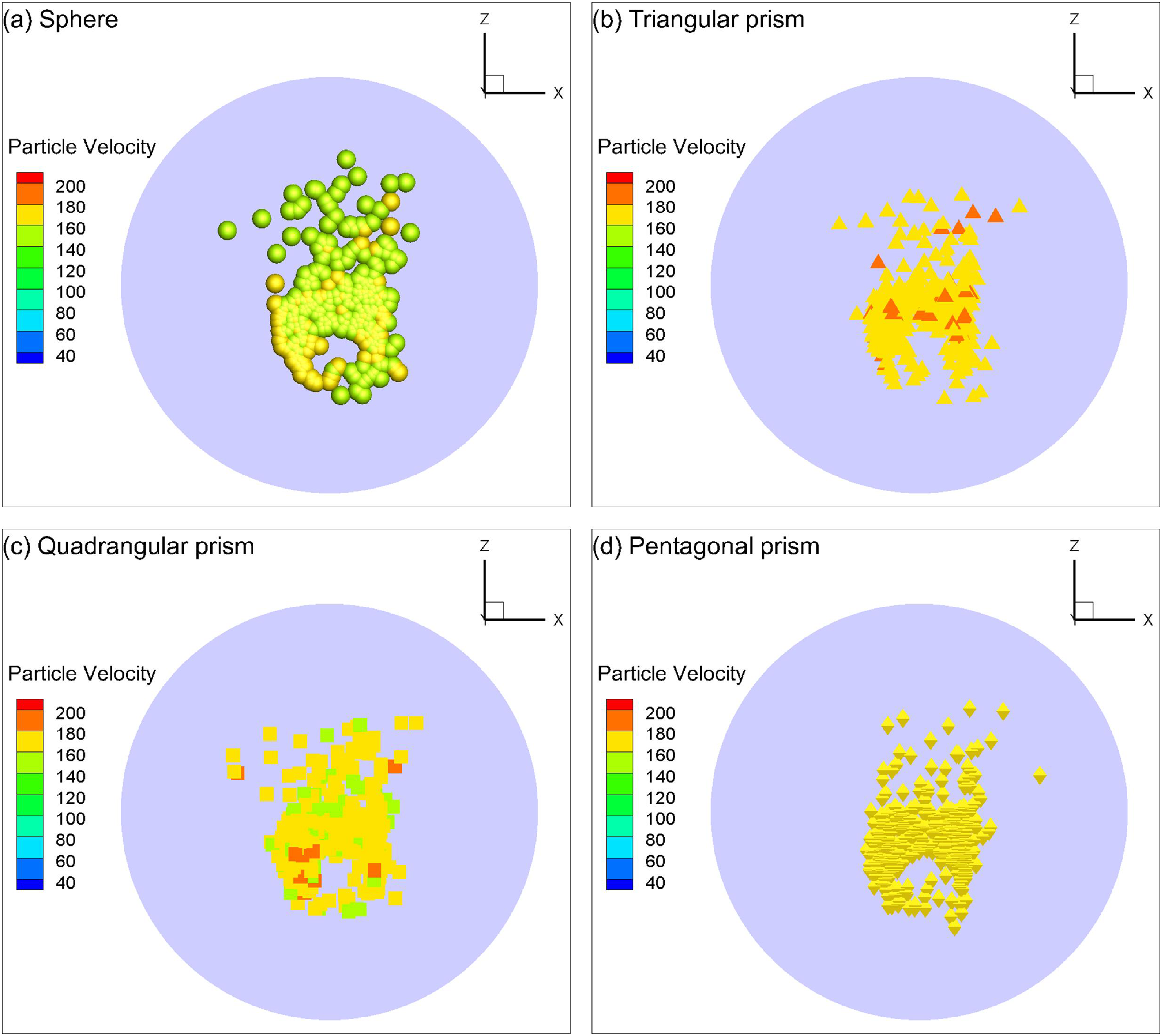
Figure 30c indicates that the ingestion rate of the four different shaped particles has an identical trend of ingestion rate with side-wind speed. However, because of the smaller aerodynamic force compared to the other shaped particles, the spherical particles are more dominated by the gravitational force, and thus the ingestion rate of the spherical particles is slightly lower than that of the irregularly shaped particles. Figure 32 indicates that there is not too much difference between the ingestion trajectories of all four shaped particles. The distribution patterns at the AIP of the inlet for all four shaped particles are also similar, but some differences in the velocity distributions are still visible, as shown in Fig. 33.
Particle distribution at the AIP of the inlet for different particle shapes at V0 = 30 m/s and Vs = 0 m/s. The mean particle size is 0.1 mm: (a) sphere, (b) triangular prism, (c) quadrangular prism and (d) pentagonal prism.

Figure 33. Long description
The image contains four scatter plots labeled (a) Sphere, (b) Triangular prism, (c) Quadrangular prism, and (d) Pentagonal prism. Each plot depicts particle velocity distributions at the aerodynamic interface plane for different particle shapes at an initial velocity of 30 meters per second and side-wind velocity of 0 meters per second. The mean particle size is 0.1 millimeters. Panel A: The scatter plot for spheres shows particle velocity distributions with a color scale ranging from 40 to 200 units. The x-axis represents the x-coordinate, and the z-axis represents the z-coordinate. The particles are colored according to their velocity, with higher velocities indicated by warmer colors. Panel B: The scatter plot for triangular prisms shows particle velocity distributions with a similar color scale. The particles are shaped as triangles and are colored according to their velocity. Panel C: The scatter plot for quadrangular prisms shows particle velocity distributions with the same color scale. The particles are shaped as squares and are colored according to their velocity. Panel D: The scatter plot for pentagonal prisms shows particle velocity distributions with the same color scale. The particles are shaped as pentagons and are colored according to their velocity. Each plot provides a visual representation of how different particle shapes affect their velocity distribution at the aerodynamic interface plane.
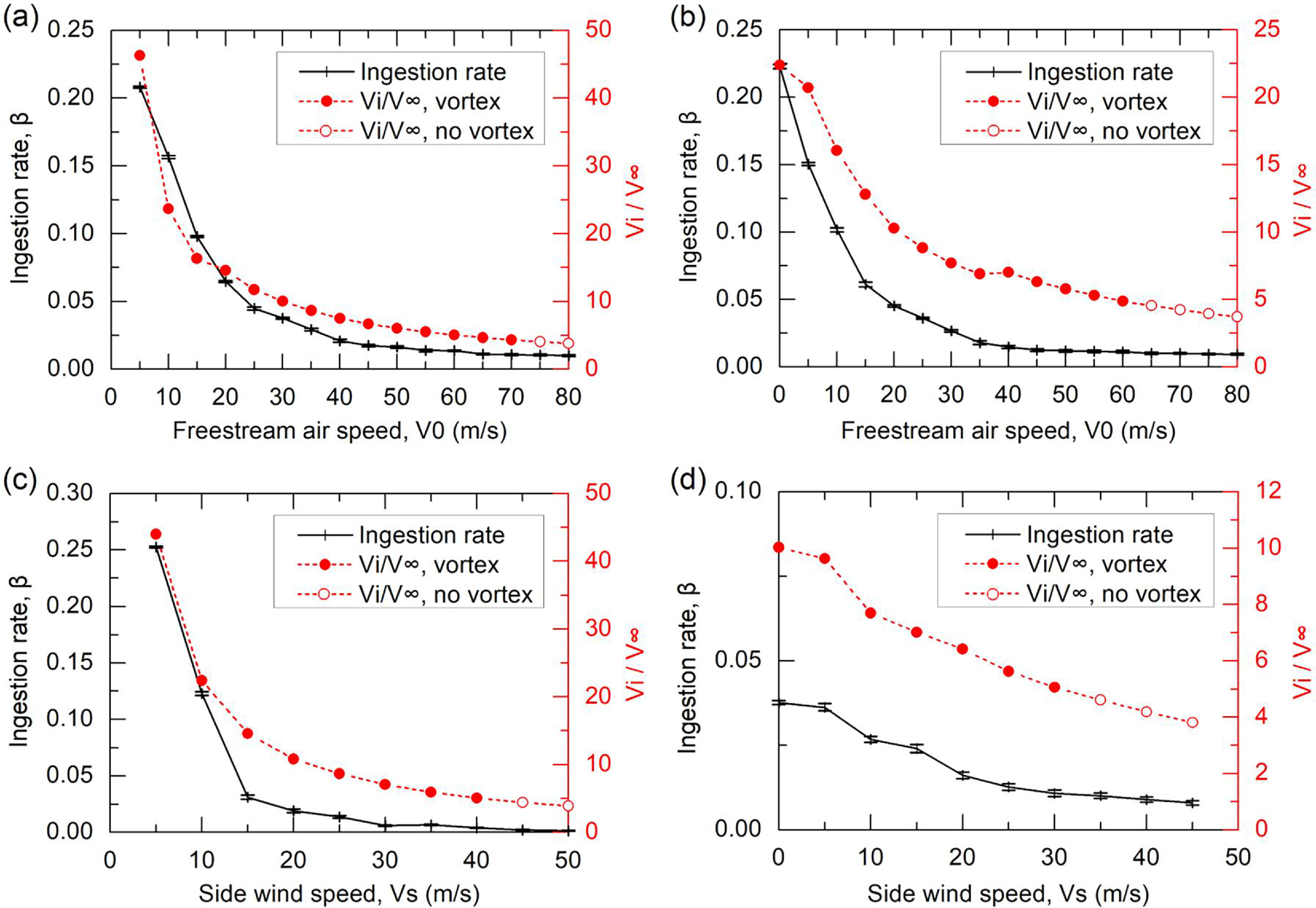
Comparison between particle ingestion rate and mass flow ratio at (a) Vs = 0 m/s, (b) Vs = 10 m/s, (c) V0 = 0 m/s, and (d) V0 = 30 m/s.

As for the influence of particle density, the ingestion rate is larger with a smaller particle density at side-wind speeds lower than 10 m/s, while the result becomes reversed as side-wind speed is beyond 10 m/s, as shown in Fig. 30d where the diameter of all the particles is fixed at 0.1 mm. Thus, a lower density means a lighter mass of the particles. At side-wind speeds lower than 10 m/s, the ground vorticity is relatively stronger; the lighter particles can better be ingested into the inlet in a manner similar to that shown in Fig. 22a. However, at side-wind speeds higher than 10 m/s, the ground vorticity is much weaker or even absent, the lighter particles are more prone to flow outside of the inlet in a manner similar to that shown in Fig. 24d, while the heavier particles obtain a higher ingestion rate thanks to the counteraction of their larger weight against the aerodynamic force. It is easily to find that the influence of particle density is similar to that of the particle size distribution law.
4.7 Sand particle-ground vortex coupling ingestion mechanism
The relation between inlet mass flow ratio (MFR) and ground clearance has been widely employed to identify the boundary between the vortex and no-vortex regimes [Reference Nakayama and Jones1, Reference Trapp and da Motta Girardi15]. The MFR is defined as
 \begin{align}{\rm{MFR}} = \frac{{{V_i}}}{{{V_\infty }}}\end{align}
where
 ${V_i}$
is the airflow velocity at the throat of the inlet and
 ${V_\infty } = \sqrt {V_0^2 + V_s^2} $
is the resultant velocity of the freestream air speed and side-wind speed.
To detect if the particle ingestion is related to the existence of the ground vortex, Fig. 34 compares the particle ingestion rate with the inlet mass flow ratio at different freestream air and side-wind speeds. It is clearly seen that the particle ingestion rate decreases with the reducing mass flow ratio for all the cases of interest, implying that the ingestion of particles is tightly related to the strength of the ground vortex. It is also interesting to find that under the circumstances of no ground vortex, the particle ingestion rate is not necessarily zero, because the stream tube can also entrain a small fraction of particles into the inlet on the premise of the ground vorticity existence, as has been revealed in Subsection 4.3. Thus, it can be concluded that both the ground vortex and stream tube are responsible for the ingestion of particles into the inlet.
Illustration of the particle-ground vortex coupling ingestion mechanisms: (a) accumulation, (b) uplift and (c) ingestion.

Figure 35. Long description
A diagram illustrating the particle-ground vortex coupling ingestion mechanisms in three stages: accumulation, uplift, and ingestion. Panel A: Accumulation. This panel shows the initial stage where particles accumulate in a low-pressure area created by ground vorticity and side wind. The freestream air flows towards the low-pressure area, and particles are concentrated in this region. Panel B: Uplift. In this stage, the ground vortex lifts the accumulated particles upwards into a stream tube. The particles are shown being uplifted from the ground into the air stream. Panel C: Ingestion. This panel depicts the final stage where the uplifted particles are ingested into the stream tube. The particles are carried away by the airflow, completing the ingestion process.
Through summarising the above findings, a mechanism of particle-ground vortex coupling ingestion can be extracted primitively. A full particle ingestion process can be divided into three stages, i.e. accumulation, uplift and ingestion, as illustrated in Fig. 35. A local low-pressure region is created by the vorticity on the ground surface, which finally develops into a ground vortex (or a pair of vortices) linking the ground and inlet or going far away from the inlet. The ground vorticity is the precondition of the occurrence of particle ingestion into an inlet. In the primary stage of particle ingestion, the approximately uniform sand particles on the sediment will be accumulated from all directions to the low-pressure region due to the pressure difference, as illustrated by Stage 1 in Fig. 35a. In the next stage, the accumulated particles will be uplifted off the ground surface by the circulation of the ground vortex when the suction force on the particle due to the low static pressure at the vortex core is greater than the gravitational force [Reference MacManus and Slaby17], as illustrated by Stage 2 in Fig. 35b. At this moment, there should be some similar regimes occurring on the particles in the ground vortex flow to those of particles entrapped in rotor downwash flow, such as saltation and bombardment [Reference Johnson, Leishman and Sydney39]. As the particles are elevated into the scope of the stream tube, they will be ingested by the stream tube into the inlet, which is named Stage 3 in Fig. 35c. Meanwhile, the particles at the vortex core will also be trapped and ingested by the ground vortex into the inlet, as long as the drag force acted by the ground vortex is strong enough to balance the gravitational force of the particles. In addition, from the perspective of velocity, according to the theory of Nielsen [Reference Nielsen40], sediment trapping will occur if the maximum swirl velocity induced by a vortex flow is larger than the settling velocity of the particle. Future studies can be carried out to validate this theory by physical tests of the sand-ground vortex coupling flow with laser sheet illumination and imaging of the flow using a high-speed digital camera, which allows for both dual-phase flow visualisation and time-resolved dual-phase particle image velocimetry (PIV) measurements of both the ground vortex flow velocity and particle movement velocity fields [Reference Johnson, Leishman and Sydney39]. On this basis, the ratio of particles ingested by the ground vortex flow to that by the stream tube can be determined.
5.0 Conclusion
In this study, a numerical simulation of the characteristics of sand ingestion into a nacelle inlet with the ground vortex has been carried out via an interior Eulerian–Lagrangian scheme named DPMTrace for particle tracking in fluids. The air phase is obtained first by solving the steady compressible RANS equation with the SST
 $k - \omega $
turbulence model, of which the flow field result is then used to initiate the calculation of the particle field. The particle tracking scheme has considered the probability distributions and the drag coefficients of four different particle shapes, as well as the probability of particle-wall rebound. Both the numerical methods for the airflow and particle dynamics were validated before the formal particle-ground vortex coupling ingestion characteristics.
The ground vortex characteristics were studied first. Four flow regimes of the ground vortex morphology are observed within the computational conditions of interest in this research, of which two regimes contain the occurrence of ground vortices extending from the ground to the inside of the inlet while the other two contain no such ground vortices. An ingestion boundary for the ground vortex existence is revealed by a map of the ground vortex characteristics. It is also found from the map that the ground vortex ingestion characteristics are more sensitive to side-wind speed than freestream air speed.
The influences of the external flow conditions (freestream air and side-wind speeds), internal flow condition (AIP Mach number), ground clearance and particle properties (size, size distribution law, shape and density) on the ingestion characteristics of sand particles are comprehensively investigated. It is found that the particle ingestion rate decreases with the increasing freestream air and side-wind speeds, with the maximum ingestion rate of about 94% occurring at both zero freestream air speed and side-wind speeds. As the AIP Mach number increases, both the ingestion rate and particle velocity at the AIP increase accordingly, since the suction effect of the inlet is increased at larger AIP Mach numbers. The particle ingestion rate generally decreases with the increasing ground clearance of the inlet because of the weakened strength of the ground vorticity. The various particle properties exert significant influences on the particle ingestion rate as well. The ingestion rate finally converged as the particle size increases to 1.2 mm. Both the particle size distribution law and particle density exhibit opposite influences on the particle ingestion rate between the two sides of the side-wind speed of 10 m/s, both of which are rooted in the mass of the particles. As for the influence of particle shape, the spherical particles show an obvious deviation of ingestion rate from the other three shaped particles due to the smallest aerodynamic force subjected. It is also noted that there are some obvious differences in the particle velocity distribution at the AIP between the four shaped particles.
As for the mechanism of particle-ground vortex coupling ingestion, it is proposed that the ingestion process contains three stages, namely accumulation, uplift and ingestion. Both the ground vortex and stream tube near the ground are found responsible for the ingestion of particles into the inlet. Further studies can be carried out to determine the ratio of particles ingested by the ground vortex flow to that by the stream tube.
Acknowledgements
This research was partially supported by the National Natural Science Foundation of China (No. 12172174 and 12572287) and the National Science and Technology Major Project of China (No. HT-J2019-V-0004-0095).
Data availability statements
Data available on request due to privacy/ethical restrictions.
Competing interests
The authors declare that they have no conflict of interest in this work.
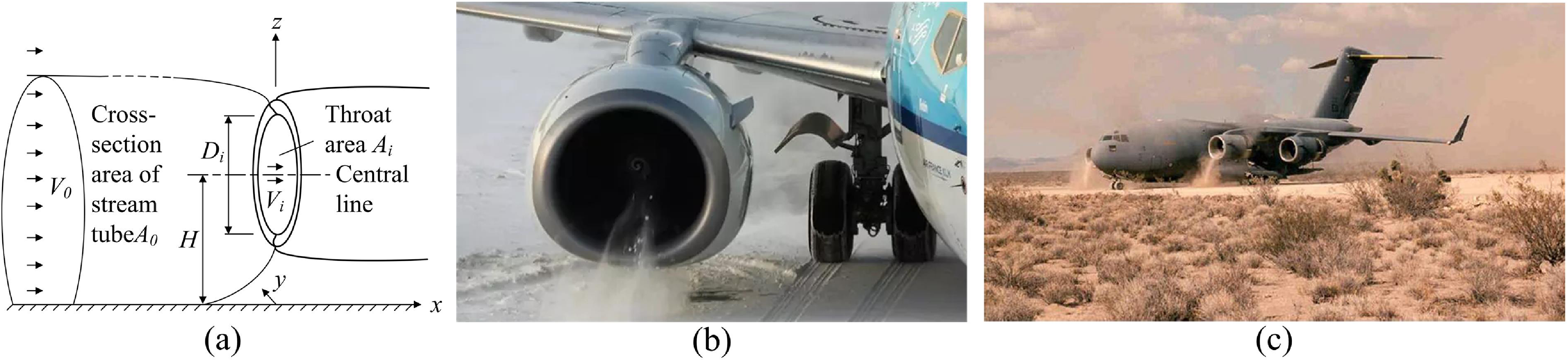
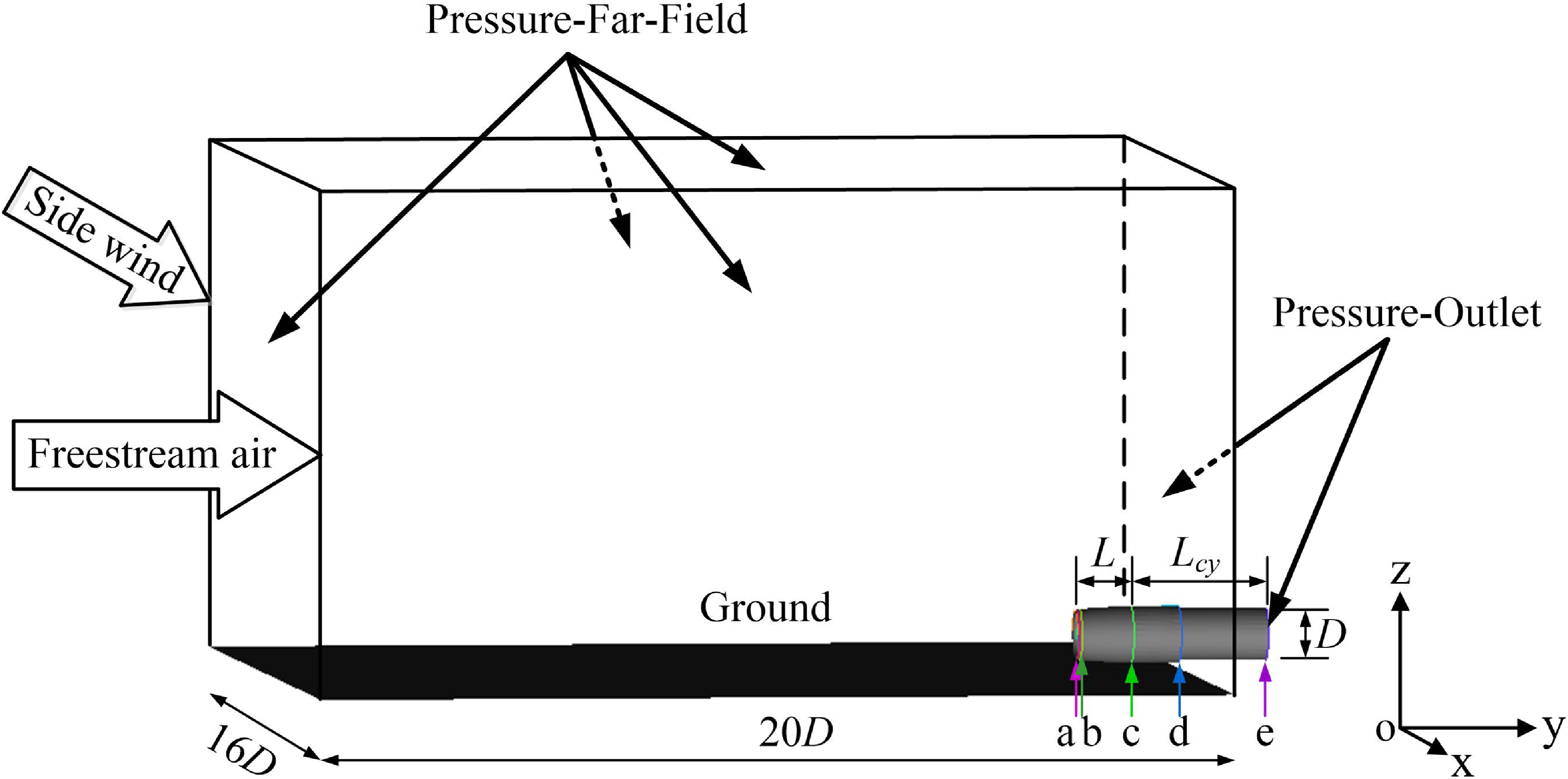
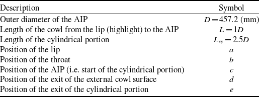
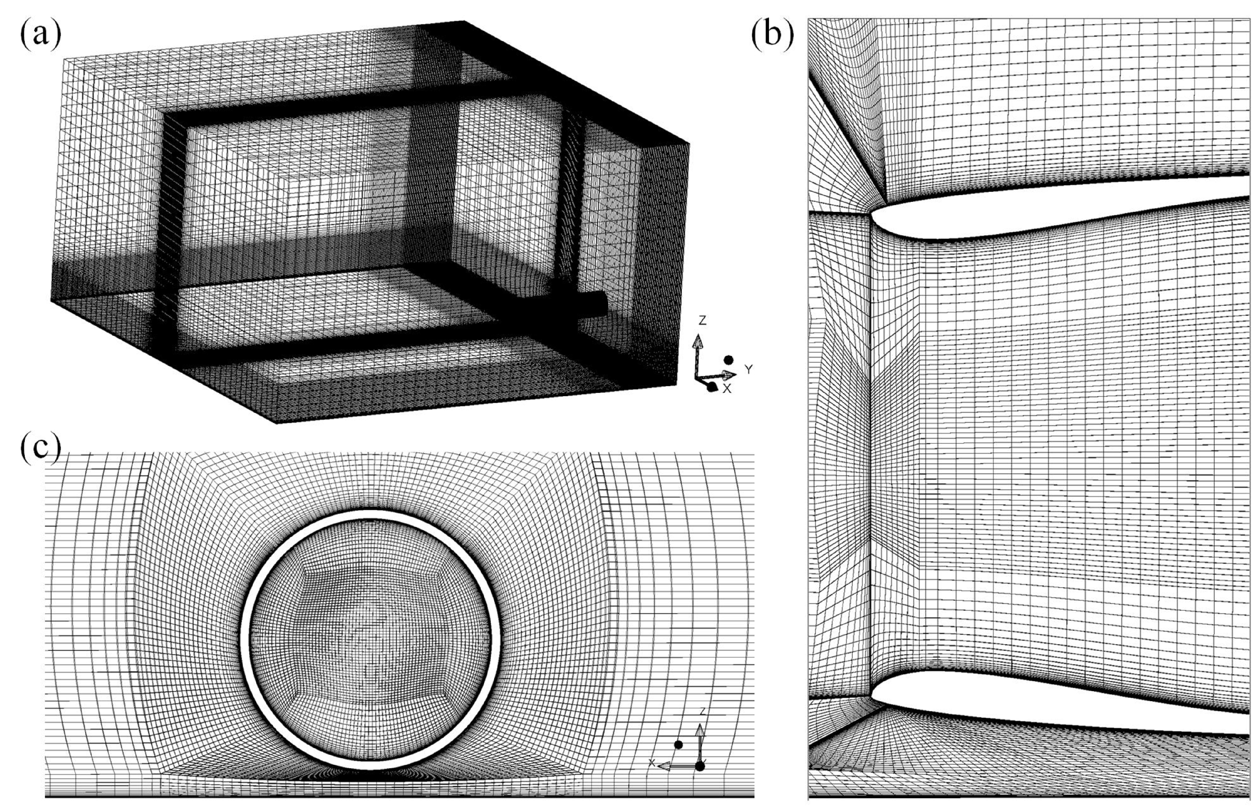
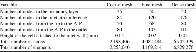
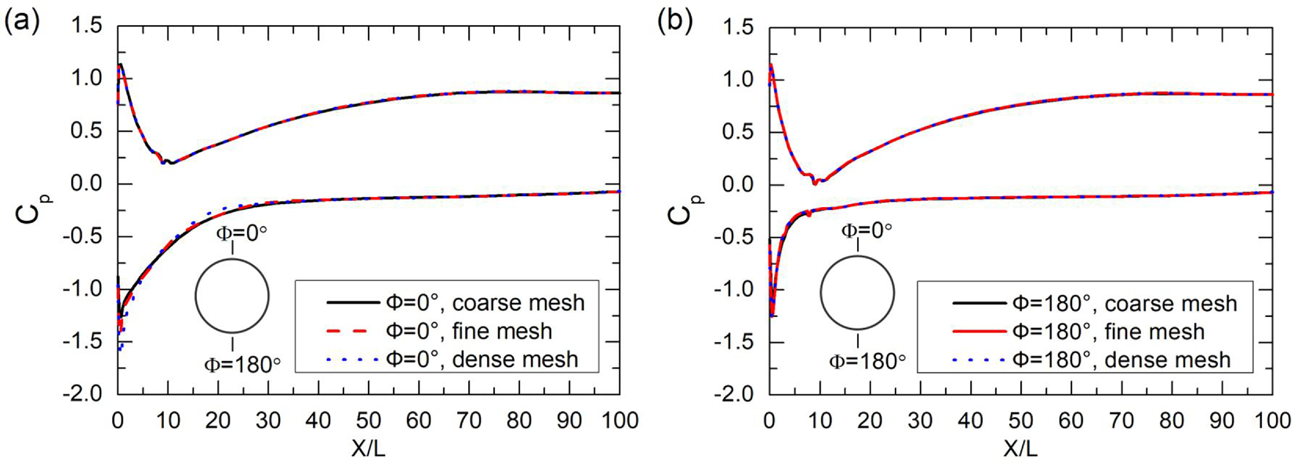
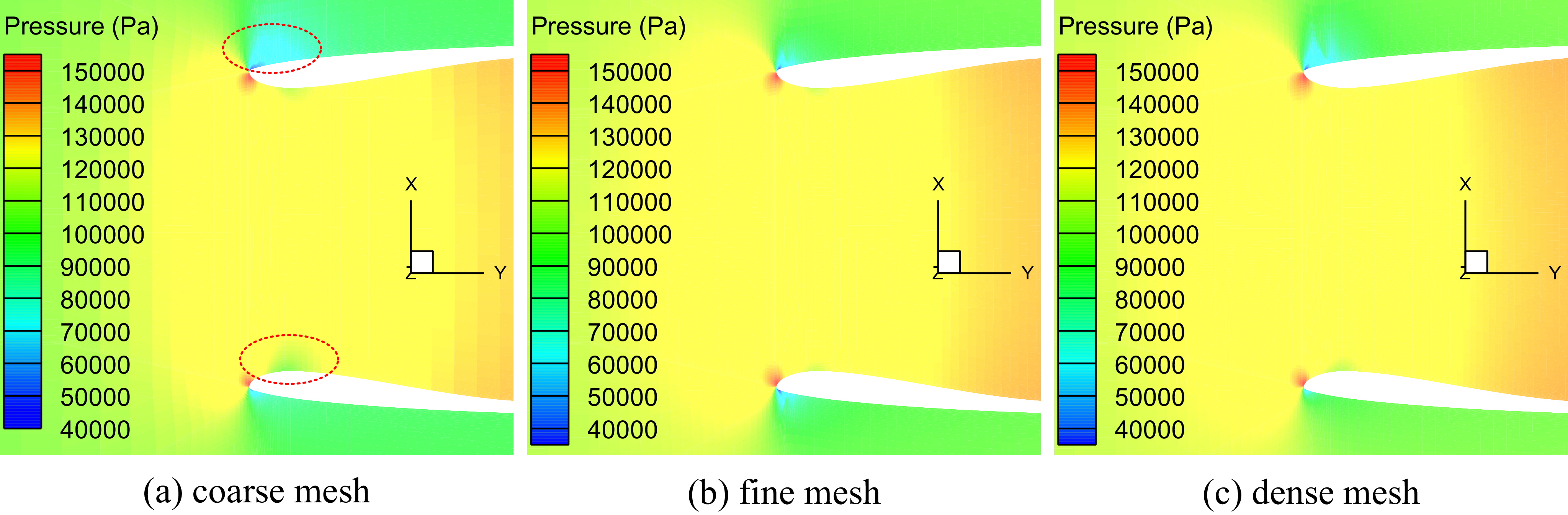
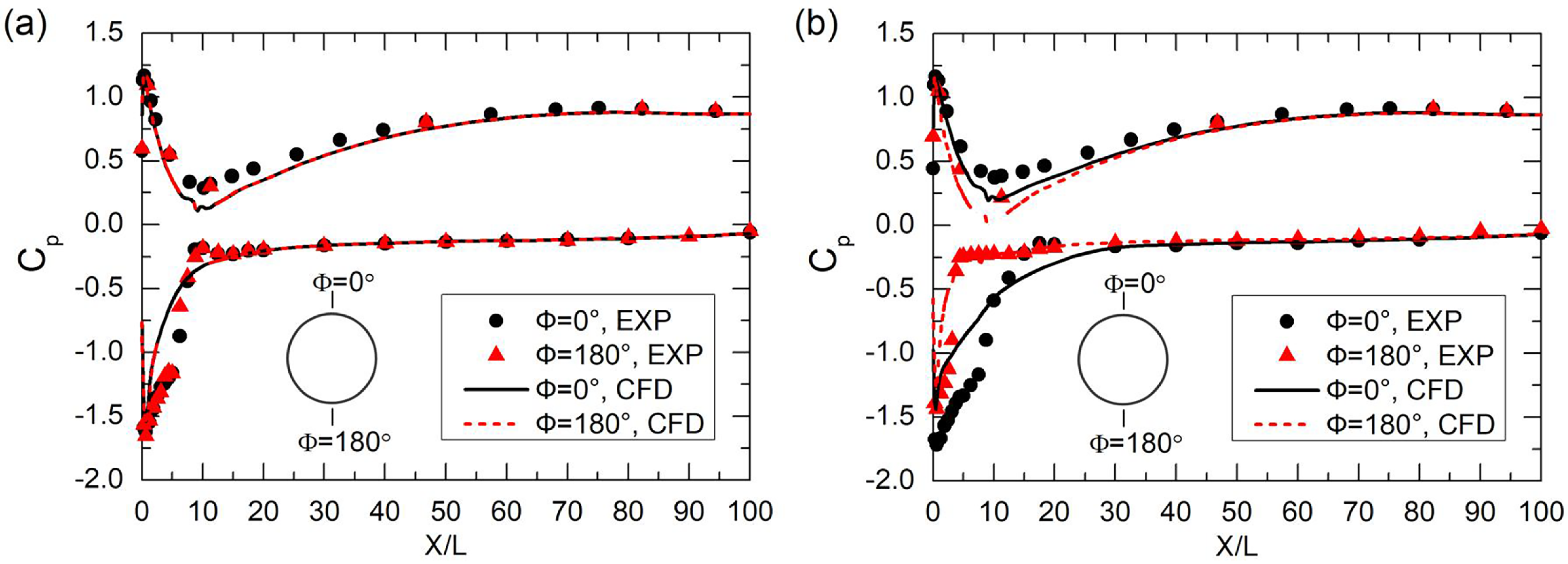
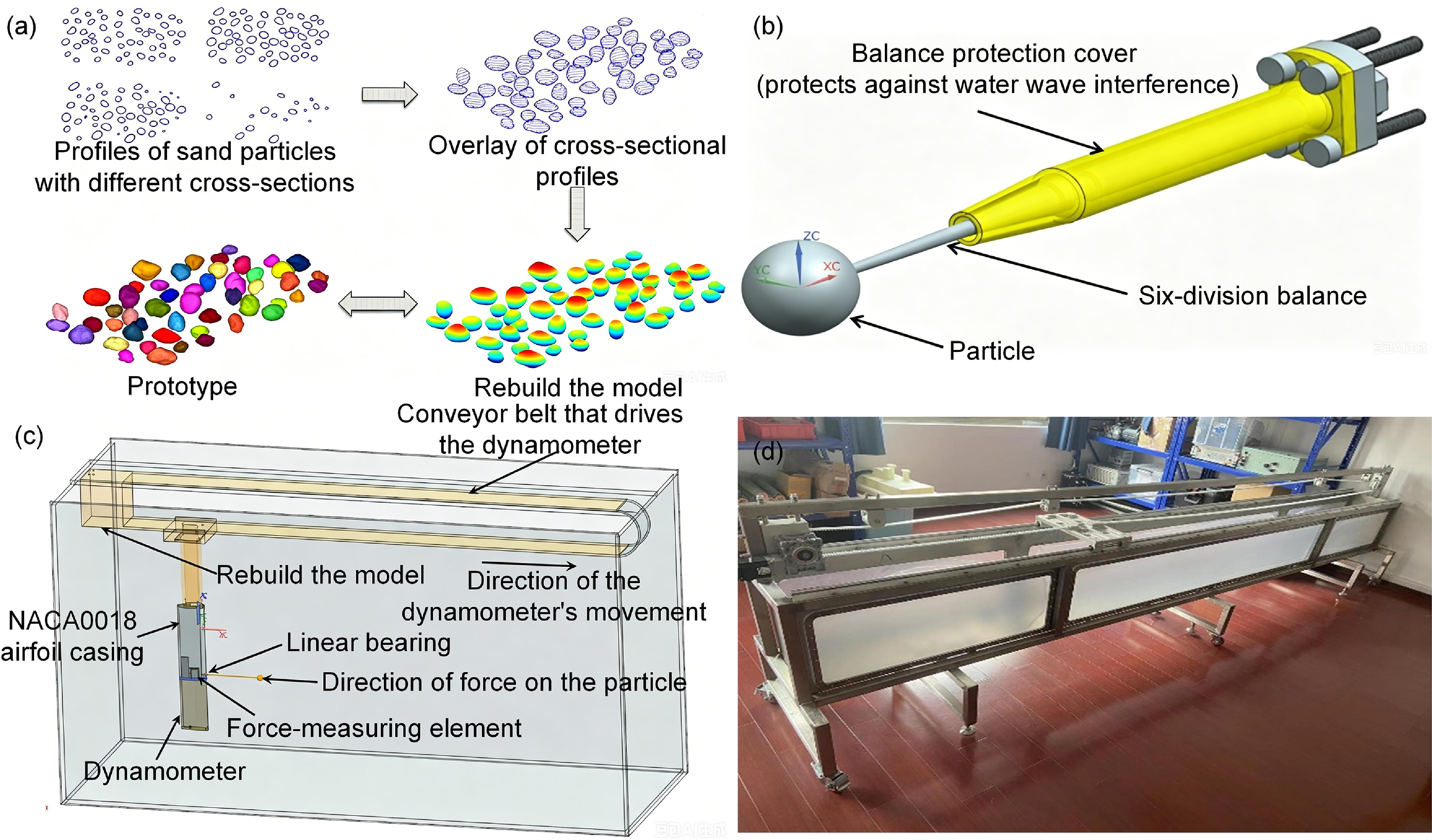
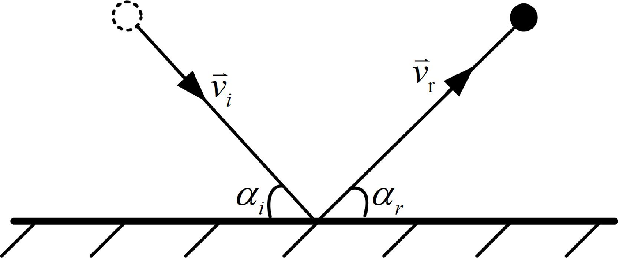
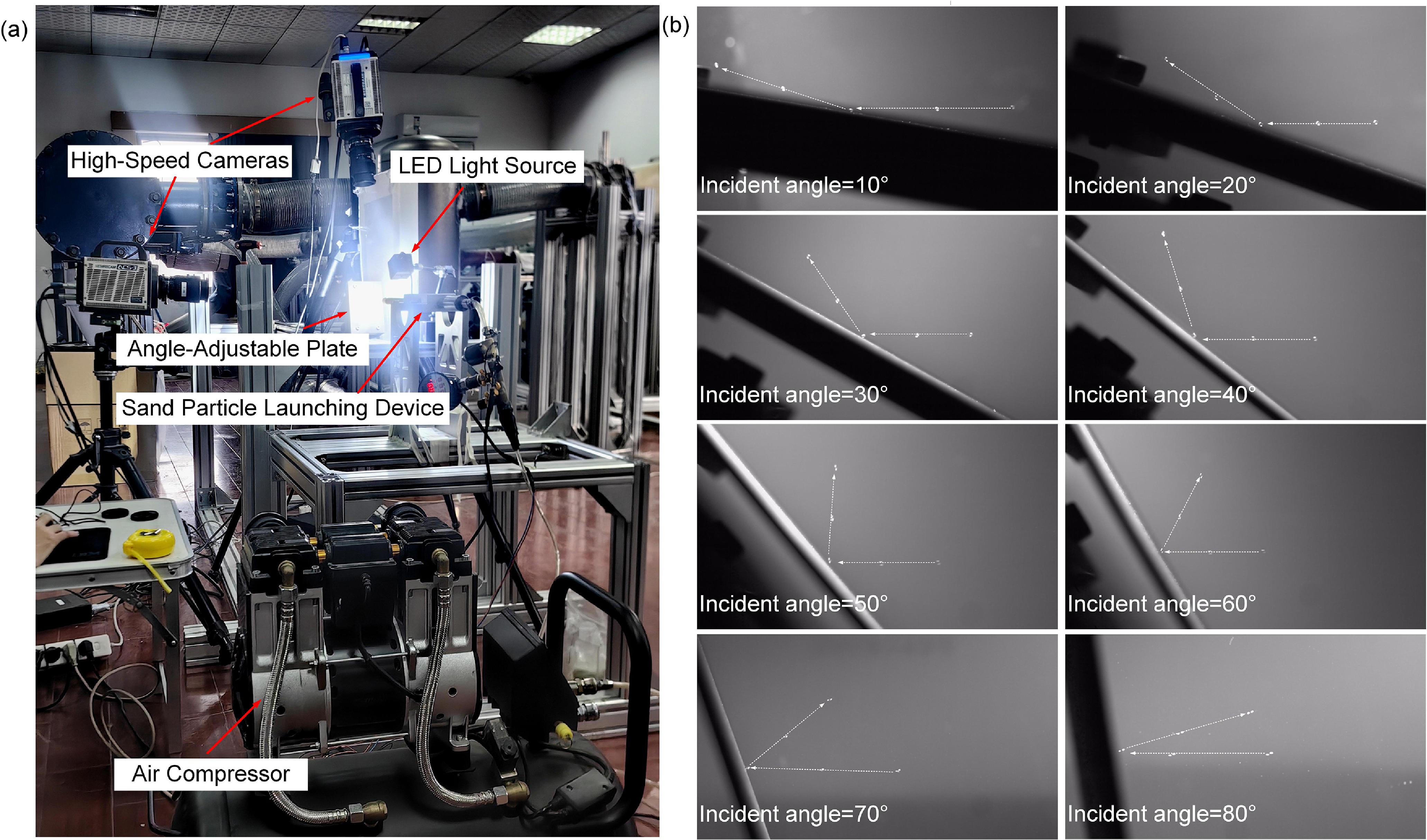


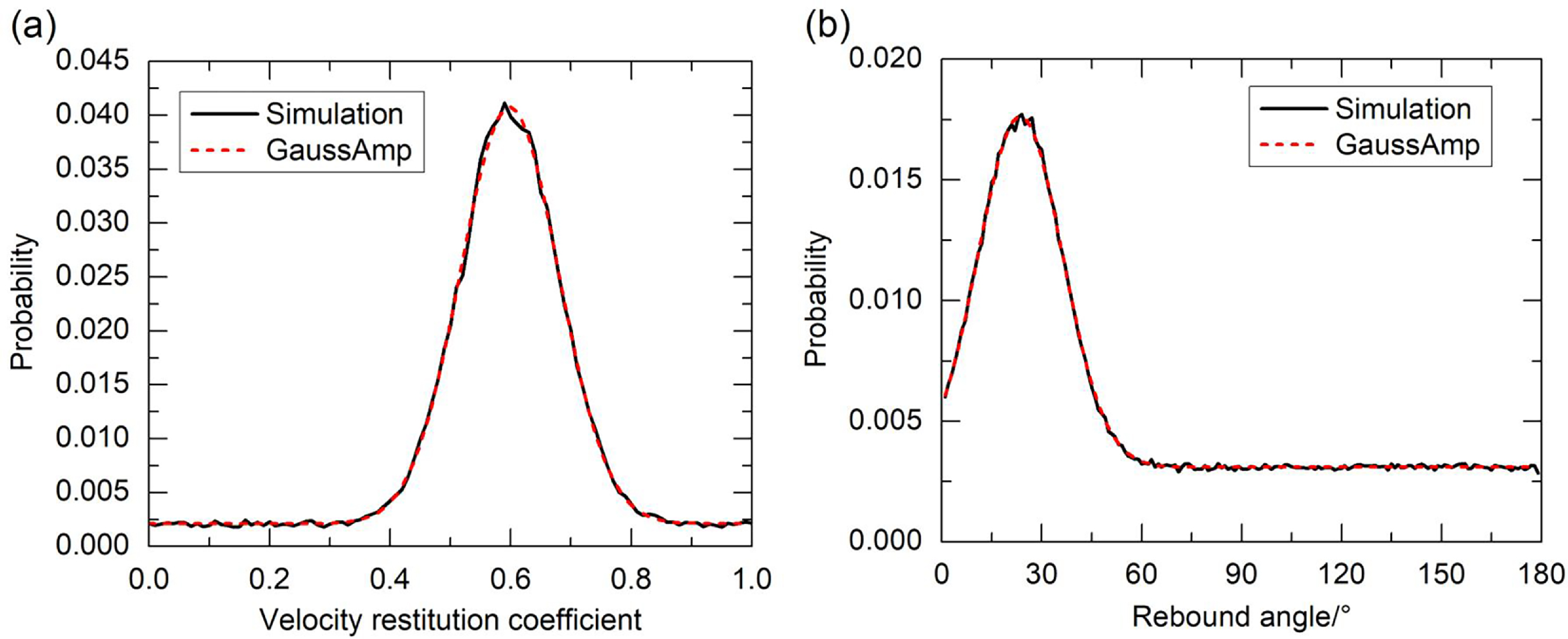
 α=40∘