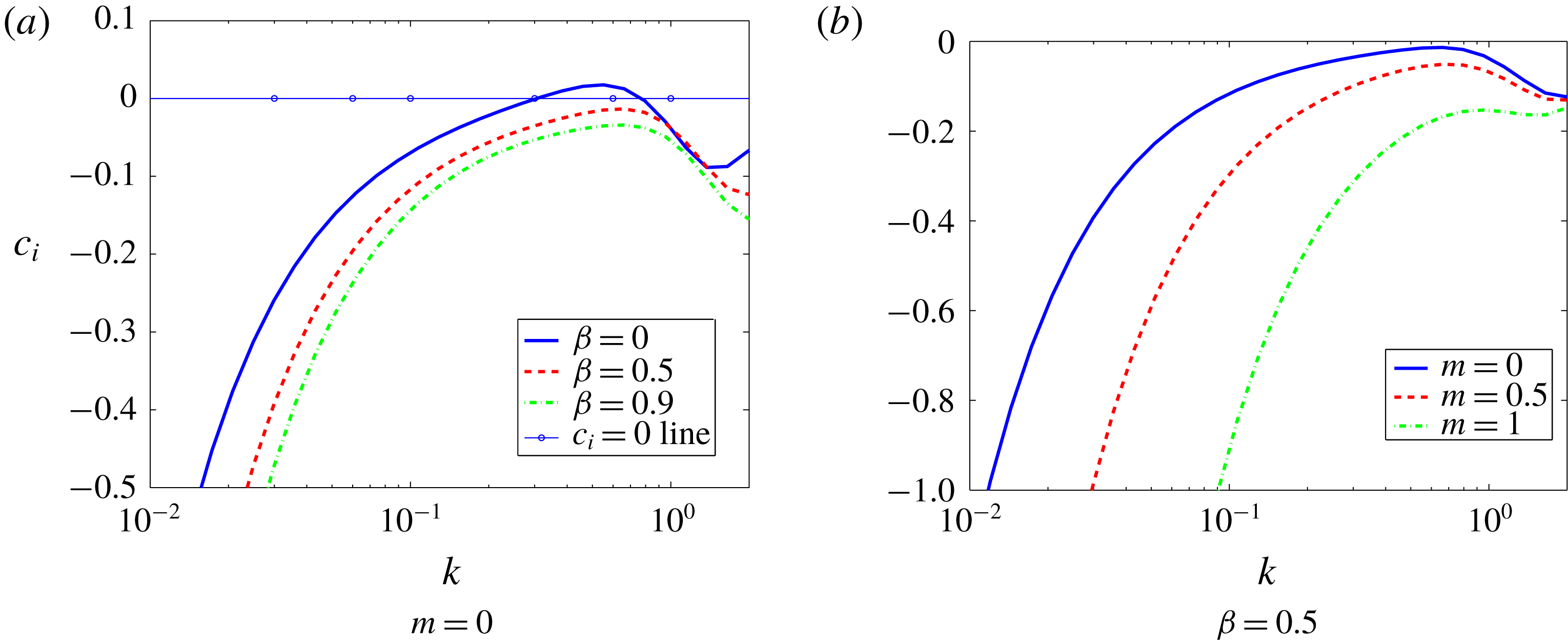
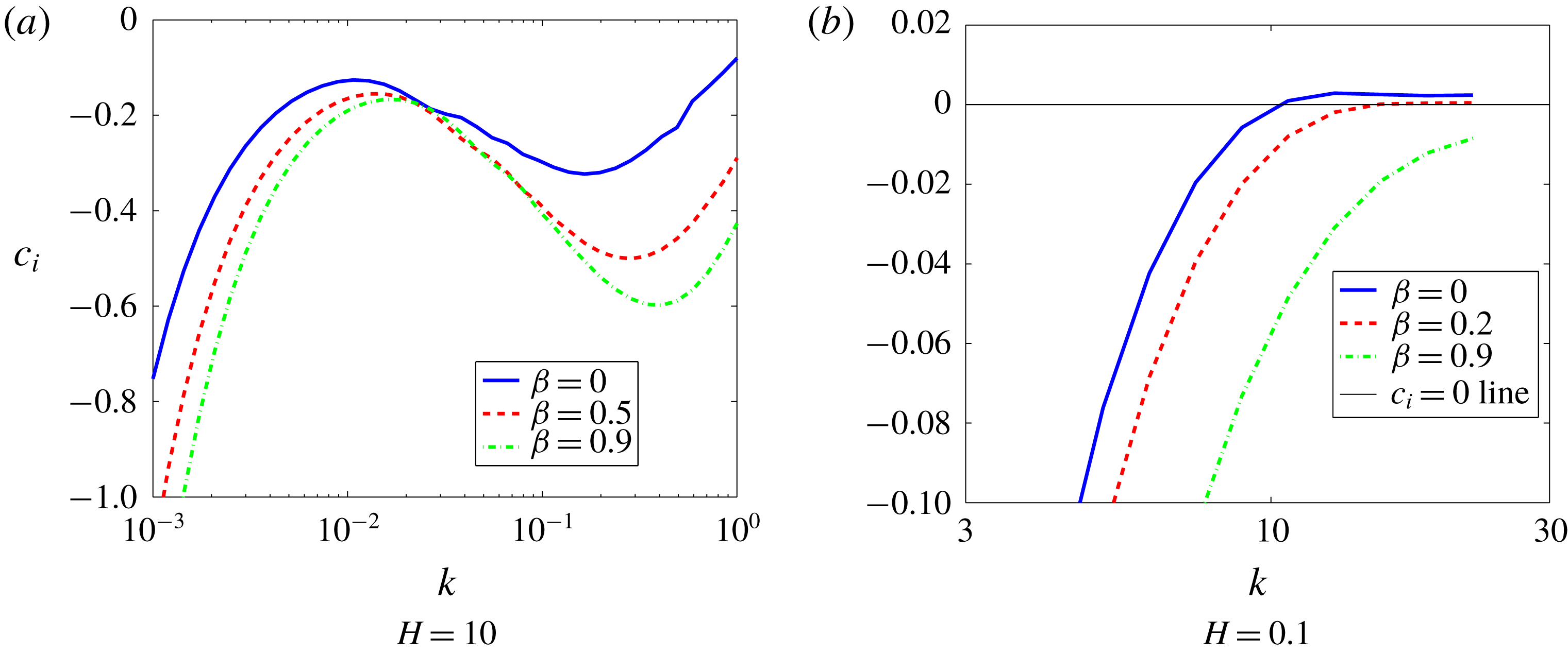
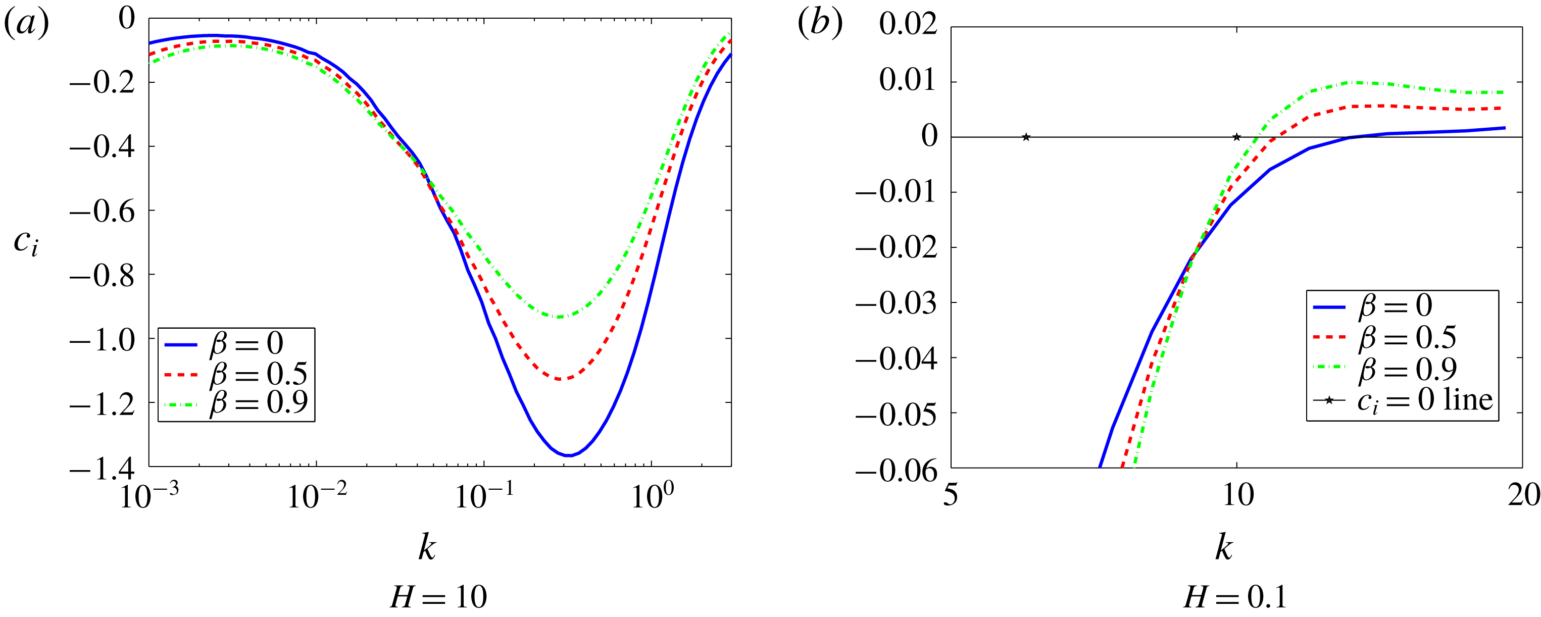
1 Introduction
The interaction between a flowing fluid and a deformable solid boundary is frequently encountered in nature, some examples of which are blood flow through blood vessels (Grotberg & Jensen Reference Grotberg and Jensen2004) and swimming of aquatic life forms. In the last two decades, it has been well established both theoretically (Shankar Reference Shankar2015) and experimentally (Kumaran Reference Kumaran2015) that the laminar–turbulent transition in tubes and channels with deformable walls is very different from their rigid counterparts. Furthermore, recent experimental findings (Eggert & Kumar Reference Eggert and Kumar2004; Shrivastava, Cussler, & Kumar Reference Shrivastava, Cussler and Kumar2008; Verma & Kumaran Reference Verma and Kumaran2012, Reference Verma and Kumaran2013; Neelamegam, Giribabu & Shankar Reference Neelamegam, Giribabu and Shankar2014; Neelamegam & Shankar Reference Neelamegam and Shankar2015; Srinivas & Kumaran Reference Srinivas and Kumaran2017) show that the destabilising role of the deformable solid can result in enhanced mixing in microscale flows.
The instabilities reported in these experiments have been predicted using classical linear stability analysis with some success (Verma & Kumaran Reference Verma and Kumaran2012, Reference Verma and Kumaran2013). The analysis involves the specification of a constitutive model for the deformable solid. However, until recently, there was no consensus on what constitutes a consistent formulation of flow-deformation coupling. A consistent formulation for carrying out the stability analysis is required in order to predict the experimental observations in an accurate and unambiguous manner. Without the use of a consistent formulation, prior studies have often found the stability of the flow, especially in pressure-driven flows in channels and tubes with deformable walls, to sensitively depend on the form of the constitutive equation used for the deformable solid (Kumaran Reference Kumaran1995b ; Gaurav & Shankar Reference Shankar2009; Patne, Giribabu & Shankar Reference Patne, Giribabu and Shankar2017) and on the manner in which the interface conditions are linearised (Gkanis & Kumar Reference Gkanis and Kumar2005; Gaurav & Shankar Reference Shankar2010; Patne et al. Reference Patne, Giribabu and Shankar2017; Patne & Shankar Reference Patne and Shankar2017). In a recent study (Patne et al. Reference Patne, Giribabu and Shankar2017), we provided a resolution to this issue, by formulating an unambiguous consistent formulation for performing stability analysis involving the coupled dynamics of fluid flow and solid deformation.
Stability analyses of flow-deformation coupling have traditionally been carried out by treating both the fluid and the deformable solid in the Eulerian framework (Chokshi & Kumaran Reference Chokshi and Kumaran2008a ,Reference Chokshi and Kumaran b ) or by treating the fluid in the Eulerian framework and the deformable solid in the Lagrangian framework (Gkanis & Kumar Reference Gkanis and Kumar2003; Gaurav & Shankar Reference Shankar2009, Reference Shankar2010). One advantage of the Eulerian–Eulerian framework is that the linearisation of the continuity conditions at the interface is an unambiguous procedure. However, traditionally, in nonlinear solid mechanics, constitutive models are formulated in the Lagrangian framework, and hence care must be taken to formulate the consistent constitutive relation in the Eulerian framework, as demonstrated by Patne et al. (Reference Patne, Giribabu and Shankar2017). This consistent Eulerian–Eulerian formulation can then be used to validate the linearisation of the interface conditions in the Eulerian–Lagrangian framework, where the formulation of the bulk constitutive relation is unambiguous. This two-way consistency of both the Eulerian and Lagrangian formulations was demonstrated in the earlier work of Patne et al. (Reference Patne, Giribabu and Shankar2017).
It was shown (Patne et al.
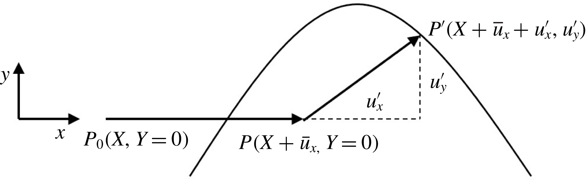
Reference Patne, Giribabu and Shankar2017) that the interface conditions in the previous studies are inconsistent owing to an incorrect Taylor series expansion about the base-state interface. Figure 1 shows the motion of the interface in the undeformed, pre-stressed and perturbed states. Gkanis & Kumar (Reference Gkanis and Kumar2005), Gaurav & Shankar (Reference Shankar2009) considered only normal displacement of the interface and hence the effective displacement of the interface in their case was
 $u_{y}^{\prime }$
. Furthermore, they Taylor expanded both fluid and and solid quantities about the unperturbed interface. It must be noted that in the Lagrangian description, because the frame moves with the particle, the Taylor expansion of the solid quantities is unnecessary. Consequently, Gaurav & Shankar (Reference Shankar2010) Taylor expanded only fluid quantities but considered effective displacement of the interface as
 $u_{y}^{\prime }$
. However, in general the interface undergoes displacement in tangential direction as well, thus, Patne et al. (Reference Patne, Giribabu and Shankar2017) considered the tangential displacement (
 $u_{x}^{\prime }$
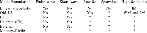
) of the interface along with the normal displacement for the Taylor expansion of the fluid quantities. This was shown to be necessary in order to cancel out the base-state terms during the linearisation of the interface conditions. This step is especially important in the linearisation of the normal stress balance in flows with a base-state pressure gradient in the flow direction. Table 1 summarises the types of the linearised interface conditions and their consequences. The disagreement highlighted in table 1 as a consequence of the incorrect formulation of the interface conditions suggests the sensitivity of the stability predictions to the change in the linearised interface conditions, hence making it necessary to formulate a consistent procedure for linearising the interface conditions.
The Taylor expansion of Patne et al. (Reference Patne, Giribabu and Shankar2017) in the tangential and normal directions to the flow generates an extra term in the normal stress continuity condition at the fluid–solid interface, as explained in § 2, which was absent in the earlier literature. It is important to justify this procedure using an independent formulation. To this end, Patne et al. (Reference Patne, Giribabu and Shankar2017) developed a consistent Eulerian formulation which does not have ambiguity in the linearised interface conditions. The consistently formulated Eulerian formulation was then used to corroborate the linearisation procedure in the Lagrangian formulation. It turns out that, without Taylor expansion in the flow direction, the results from the consistent Eulerian and Lagrangian formulations do not agree, thereby justifying the importance of two alternative formulations that nevertheless yield the same results.
A schematic of the fluid–solid interface in the base and perturbed states. Here,
 $P_{0}(X,Y=0),P(X+\bar{u}_{x},Y=0)$
and
 $P^{\prime }(X+\bar{u}_{x}+u_{x}^{\prime },u_{y}^{\prime })$
are respectively the positions of the representative particle at the interface in the undeformed, pre-stressed and perturbed states. Also,
 $u_{x}^{\prime }$
and
 $u_{y}^{\prime }$
are respectively the perturbation displacements of the interface from the base-state position in the
 $x$
and
 $y$
directions and
 $\bar{u}_{x}$
is the base-state displacement of the interface.

A summary of the linearisation procedures used in the literature for the interface conditions in pressure-driven flows through deformable channels/tubes. The second, third and fourth columns respectively refer to the Taylor expansion of base-state quantities, direction(s) of Taylor expansion and instabilities predicted as a consequence of the linearisation of the interface conditions. Question mark indicates the unanswered questions.

In the present work, we use the consistent formulation to assess the validity of the existing results in the literature concerning the stability of fluid flow through deformable tubes and channels. We demonstrate that the use of the consistent formulation drastically changes some of the conclusions in the existing literature. We further examine the role of three-dimensional perturbations on the nature of the solid constitutive model used in the stability of flow through deformable channels. Also, theoretically it remains an open question whether a more complex model such as the Mooney–Rivlin model will exhibit qualitatively new instabilities in addition to those present in the neo-Hookean model. Therefore, in the present study, we also address the question of what is the ‘minimal’ (nonlinear) constitutive model for the deformable solid wall that adequately captures all the instabilities in the system. We next briefly review the relevant literature and motivate the objectives of the present work alongside.
1.1 Planar flows
Hains & Price (Reference Hains and Price1962), Gajjar & Sibanda (Reference Gajjar and Sibanda1996), Davies & Carpenter (Reference Davies and Carpenter1997) studied the stability of plane Poiseuille flow through a deformable channel by using plate-and-spring model for the deformable walls which assumes that the solid is made up of plates connected by Hookean springs. Hains & Price (Reference Hains and Price1962) predicted a stabilising effect on the Tollmien–Schlichting (TS) instability (that exists for plane Poiseuille flow within rigid walls) of the deformable walls but Gajjar & Sibanda (Reference Gajjar and Sibanda1996), Davies & Carpenter (Reference Davies and Carpenter1997) predicted destabilising effect. The disagreement could be ascribed to the assumption of Hains & Price (Reference Hains and Price1962) who assumed deformable walls as membranes with zero damping and a finite value of tension.
The plate-and-spring model is not the most appropriate description of the deformable solid since continuum mechanics provides more realistic models (such as linear viscoelastic and neo-Hookean models) to describe the behaviour of the deformable solid under a stress field (Malvern Reference Malvern1969; Holzapfel Reference Holzapfel2000). Motivated by the experimental work of Krindel & Silberberg (Reference Krindel and Silberberg1979), Kumaran, Fredrickson & Pincus (Reference Kumaran, Fredrickson and Pincus1994) theoretically studied the stability of the plane Couette flow past a linear viscoelastic solid in the creeping-flow limit and predicted the presence of the ‘finite-wave’ instability which exists for
 $0.1<k<1$
for
 $H>1$
where
 $k$
and
 $H$
are respectively the wavenumber and the ratio of the solid to fluid thickness. The theoretical predictions of Kumaran et al. (Reference Kumaran, Fredrickson and Pincus1994) were later found to be in good agreement with the experimental observations of Kumaran & Muralikrishnan (Reference Kumaran and Muralikrishnan2000).
Recognising the inapplicability of the linear elastic solid model for the finite deformations, Gkanis & Kumar (Reference Gkanis and Kumar2003) studied the stability of inertialess plane Couette flow of a Newtonian fluid past a deformable wall while using a nonlinear and material frame-invariant neo-Hookean model applicable for finite base-state deformations in the solid. The analysis of Gkanis & Kumar (Reference Gkanis and Kumar2003) predicted, in addition to the finite-wave instability predicted using the linear elastic model, a new high-wavenumber instability present for
 $k>5$
(henceforth called as ‘short-wave instability’) which becomes the critical mode for
 $H<1$
in the creeping-flow limit, while for
 $H>1$
, the finite-wave instability remains the most dominant mode. The applicability of the neo-Hookean model to describe the solid deformation was experimentally verified by Neelamegam et al. (Reference Neelamegam, Giribabu and Shankar2014) for stability of plane Couette flow past a two-layered gel, where they showed quantitative agreement between theory and experiments.
Gkanis & Kumar (Reference Gkanis and Kumar2005) subsequently studied the pressure-driven flow past a neo-Hookean solid in the creeping-flow limit and predicted the existence of the finite-wave and short-wave instabilities similar to the plane Couette flow past a neo-Hookean solid. However, Gaurav & Shankar (Reference Shankar2010), Patne & Shankar (Reference Patne and Shankar2017) argued that the finite-wave instability predicted by Gkanis & Kumar (Reference Gkanis and Kumar2005) for plane Poiseuille flow past a neo-Hookean solid is a consequence of inconsistent interface conditions, as explained in § 3.1. The short-wave instability predicted by Gkanis & Kumar (Reference Gkanis and Kumar2005) is present in pressure-driven plane channel flow even after the incorporation of consistent linearised interface conditions. The analysis of Gaurav & Shankar (Reference Shankar2010) also predicted a new class of unstable modes at low Reynolds number (
 $Re$
). Experiments on plane Poiseuille flow past a deformable solid by Verma & Kumaran (Reference Verma and Kumaran2013) found good agreement with theory provided that the solid is modelled using the neo-Hookean model and that the change in the shape of the deformable wall due to the decrease in pressure along the length of the channel and its effect on the base-state velocity profile is considered, justifying the usefulness of the neo-Hookean model.
1.2 Hagen–Poiseuille flow
Kumaran (Reference Kumaran1995b ) studied the stability of inertialess Hagen–Poiseuille flow through a linear viscoelastic tube and predicted a finite-wave instability similar to that in plane Couette flow. Similar to plane Poiseuille flow through a neo-Hookean channel, for inertialess Hagen–Poiseuille flow through a neo-Hookean tube, Gaurav & Shankar (Reference Shankar2009) predicted the absence of the finite-wave instability at variance with the prediction of Kumaran (Reference Kumaran1995b ). The disagreement between the predictions of Gaurav & Shankar (Reference Shankar2010) and Kumaran (Reference Kumaran1995b ) was ascribed to the inapplicability of the linear viscoelastic model to finite base-state deformations, thereby showing the sensitivity of the stability results to the solid model. However, a short-wave instability similar to the one predicted by Gkanis & Kumar (Reference Gkanis and Kumar2005) is present even in the case of flow through a neo-Hookean tube. Interestingly, similar to plane Poiseuille flow (Gaurav & Shankar Reference Shankar2010), even for Hagen–Poiseuille flow, Gaurav & Shankar (Reference Shankar2009) found a low Reynolds number instability. However, the linearised interface conditions used by Gaurav & Shankar (Reference Shankar2009) were later shown to be inconsistent by Patne et al. (Reference Patne, Giribabu and Shankar2017). Verma & Kumaran (Reference Verma and Kumaran2012) performed experiments on the stability of Hagen–Poiseuille flow through a neo-Hookean tube and, by considering non-negligible deformation of the tube, Verma & Kumaran (Reference Verma and Kumaran2015) showed agreement between theory and experiments. It must be noted that to derive the base-state velocity profile for the fluid, Verma & Kumaran (Reference Verma and Kumaran2012, Reference Verma and Kumaran2015) used experimentally measured deformation in the solid for the simulations to calculate the base-state velocity profile.
The above discussion for fluid flow through neo-Hookean channels and tubes shows that a change in interface conditions or a change in the solid constitutive model has drastic consequences for the predictions of the stability analysis. Hence, it becomes essential to employ a formulation that is consistent both in the constitutive model for the solid as well as in the linearisation of the interface conditions. Although experiments by Verma & Kumaran (Reference Verma and Kumaran2012, Reference Verma and Kumaran2013) showed the utility of the neo-Hookean model, the experiments were performed for
 $Re>300$
, where nonlinear models, even if not formulated in a consistent manner, asymptotically approach the linear viscoelastic model owing to the dominance of the inertial effects and the low values of base-state deformation in the solid at the critical conditions for instability. It must be noted that in many biological processes such as blood flow through smaller blood vessels and capillaries, the Reynolds number ranges from
 $10^{-3}$
to
 $6000$
(Giribabu & Shankar Reference Giribabu and Shankar2017). Realising the necessity for consistent formulation, Patne et al. (Reference Patne, Giribabu and Shankar2017) developed consistent Eulerian and Lagrangian formulations, the salient features of which are discussed below.
1.3 The Eulerian and Lagrangian formulations
The studies of Gkanis & Kumar (Reference Gkanis and Kumar2003, Reference Gkanis and Kumar2005), Gaurav & Shankar (Reference Shankar2009, Reference Shankar2010), Verma & Kumaran (Reference Verma and Kumaran2012, Reference Verma and Kumaran2013) use the undeformed state of the solid as the reference state while deriving base-state and perturbed-state quantities. Thus only two states, viz., undeformed and perturbed states are needed while formulating the problem. Hereafter, the formulation used by Gaurav & Shankar (Reference Shankar2009, Reference Shankar2010) will be referred as the ‘old L2’ formulation. Chokshi & Kumaran (Reference Chokshi and Kumaran2008a
) proposed an alternative Lagrangian formulation which uses all three states of the solid, viz., undeformed, deformed (or pre-stressed) and perturbed states of the solid while formulating the problem. Further, Chokshi & Kumaran (Reference Chokshi and Kumaran2008a
), while analysing weakly nonlinear stability of plane Couette flow past a neo-Hookean solid, showed agreement between their Eulerian and Lagrangian formulations. However, this agreement was later shown (Patne et al.
Reference Patne, Giribabu and Shankar2017) to be a special case that holds only for plane Couette flow subjected to two-dimensional disturbances. The Eulerian formulation of Chokshi & Kumaran (Reference Chokshi and Kumaran2008a
) will be referred henceforth as the ‘Eulerian (CK)’ formulation. The constitutive relation employed for the Eulerian (CK) formulation was derived in analogy with a Newtonian fluid (Patne et al.
Reference Patne, Giribabu and Shankar2017), but consistency demands that the constitutive relation should be derived from a strain energy function. Considering the importance of the constitutive models that have been used in the literature, in table 2, we list the three nonlinear models, viz., the standard neo-Hookean model (Holzapfel Reference Holzapfel2000), neo-Hookean model of Chokshi & Kumaran (Reference Chokshi and Kumaran2008a
) for the Eulerian (CK) formulation and the Mooney–Rivlin (Holzapfel Reference Holzapfel2000) model in both the Eulerian and Lagrangian frames of reference. The linear superposition of the first two rows (the neo-Hookean and Eulerian (CK) formulations) in table 2 is the third row (Mooney–Rivlin model) with the substitution
 $C_{1}=C_{2}=G/2$
, where
 $C_{1}$
and
 $C_{2}$
are the Mooney–Rivlin constants. Although, for realistic materials
 $C_{1}>C_{2}\neq G/2$
(Macosko Reference Macosko1994).
The (dimensional) nonlinear solid models in their Eulerian and Lagrangian forms. Here,
 $\unicode[STIX]{x1D748},\unicode[STIX]{x1D644},\unicode[STIX]{x1D641}$
and
 $\unicode[STIX]{x1D65B}$
are respectively Cauchy stress, identity, Lagrangian deformation gradient and Eulerian deformation gradient tensors. Also,
 $p_{g}$
and
 $G$
are respectively the pressure field and shear modulus of the solid.

The inconsistency of the Eulerian (CK) formulation was then resolved in the study of Patne et al. (Reference Patne, Giribabu and Shankar2017) by proposing a consistent Eulerian formulation (first row and second column of table 2) using the relationship between the deformation gradients in the Eulerian and Lagrangian frames of reference. The validity of the (consistent) Eulerian formulation was demonstrated by showing that the results agree (for different flow geometries) with the Lagrangian (L3) formulation. Also the Lagrangian formulation of Chokshi & Kumaran (Reference Chokshi and Kumaran2008a ) was inconsistent, as the base state was a function of the undeformed state coordinates, but consistency demands the base state to be a function of the pre-stressed-state coordinates. Therefore, Patne et al. (Reference Patne, Giribabu and Shankar2017) proposed a consistent Lagrangian formulation (henceforth referred as the ‘L3’ formulation) and showed the advantage of using the L3 formulation over the L2 formulation by proving the consistency of the former while deriving interface conditions.
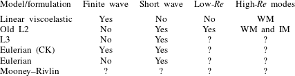
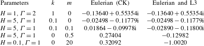
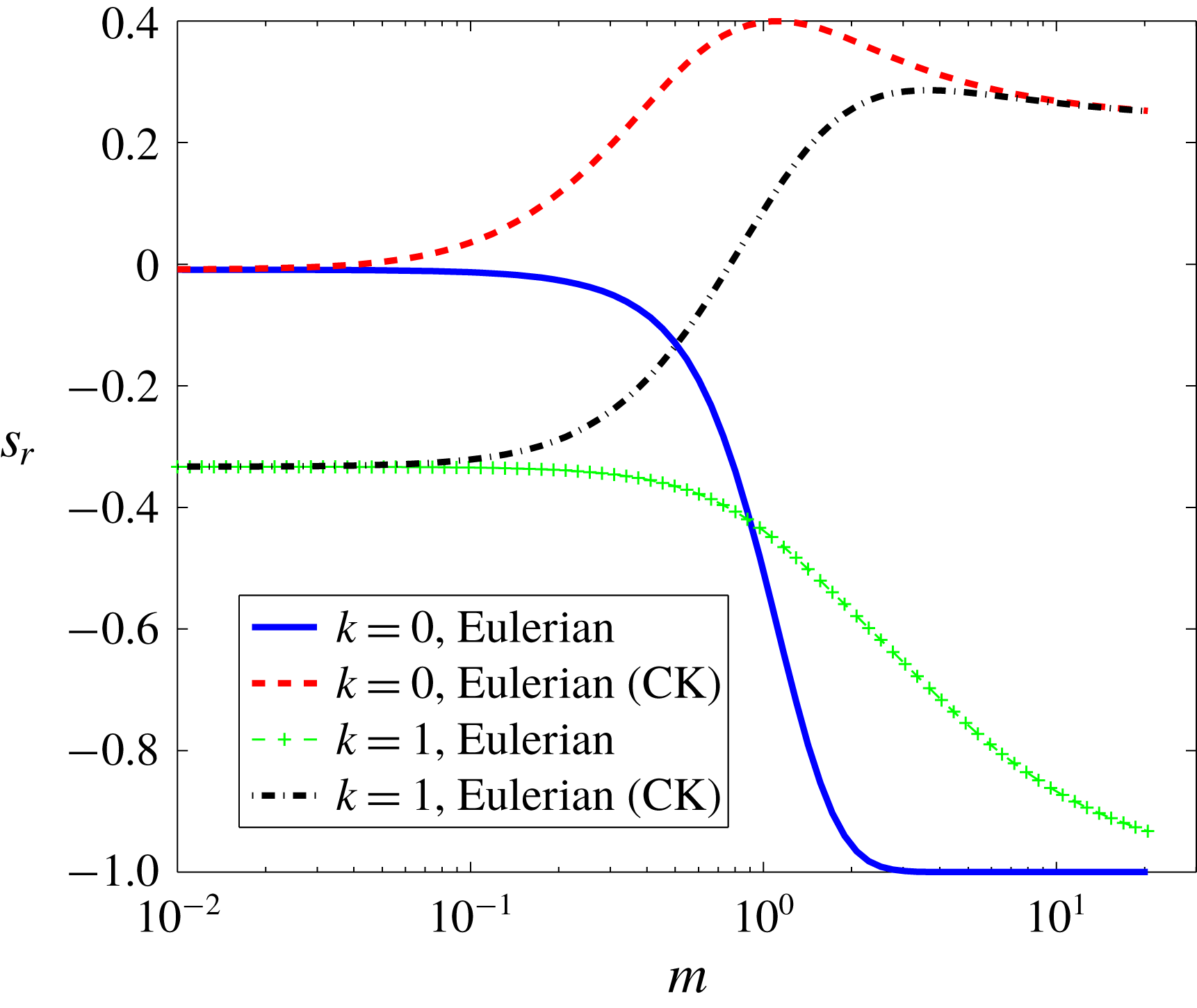
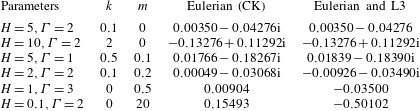
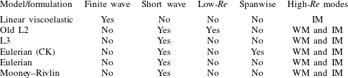
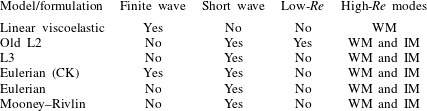
However, Patne et al. (Reference Patne, Giribabu and Shankar2017) did not explore the consequences of using the consistent interface conditions for the stability of the plane Poiseuille flow through a neo-Hookean channel and Hagen–Poiseuille flow through a neo-Hookean tube, as highlighted in tables 3 and 4 by question marks. Also, Patne et al. (Reference Patne, Giribabu and Shankar2017) demonstrated the mathematical equivalence between the Eulerian and Eulerian (CK) formulations subjected to two-dimensional disturbances and alluded to the possibility of disagreement between the two formulations if three-dimensional disturbances are considered for planar flows past a neo-Hookean solid. Table 2 shows that the linear combination of the constitutive relations of the Eulerian (CK) and Eulerian formulations is the Mooney–Rivlin model. As the Eulerian (CK) formulation predicts finite-wave instability in the creeping-flow limit for Hagen–Poiseuille flow through a neo-Hookean tube subjected to axisymmetric disturbances at variance with the Eulerian formulation (Patne et al. Reference Patne, Giribabu and Shankar2017), therefore, the question arises as to whether there will be a finite-wave instability for Hagen–Poiseuille flow as well if the solid is modelled using the Mooney–Rivlin model. Tables 3 and 4 summarise the current state of understanding of instabilities in flow through deformable channels and tubes, along with the questions that are unanswered.
Instabilities exhibited by various models or formulations for plane Poiseuille flow through a channel with deformable wall(s). WM and IM respectively refer to the wall and inviscid modes. Question marks indicate the unanswered questions.

Instabilities exhibited by various models or formulations for Hagen–Poiseuille flow through a deformable tube subjected to axisymmetric disturbances.

In the present work, we address the above questions and study the implications of employing consistent solid models and interfacial conditions to determine the minimal solid model to study the hydrodynamic stability past deformable surfaces. Also, the studies mentioned above discuss the stability of the fluid flows past deformable surfaces subjected to two-dimensional disturbances although Squire’s theorem, which shows that the two-dimensional disturbances are more unstable than three-dimensional disturbances for planar shear flows (Drazin & Reid Reference Drazin and Reid1981), is not applicable for deformable channels. Here, we show that Squire’s theorem is practically valid for flow past neo-Hookean deformable solid surfaces, but only when a consistent formulation is employed. Our stability predictions for flow through neo-Hookean channels and tubes are also compared with the previous studies of Gaurav & Shankar (Reference Shankar2009, Reference Shankar2010) in order to assess which aspects of the earlier results need to be revised in view of the consistent formulation.
The rest of the paper is organised as follows. In § 2, we derive the base-state quantities and linearised perturbation equations for plane Poiseuille flow through a neo-Hookean channel and Hagen–Poiseuille flow through a Mooney–Rivlin tube. Section 3 presents the important results for planar flows past neo-Hookean and Mooney–Rivlin solids subjected to two- and three-dimensional disturbances along with Hagen–Poiseuille flow through neo-Hookean and Mooney–Rivlin tubes subjected to axisymmetric disturbances. In § 4 we compare and contrast the instabilities predicted here and those predicted in the previous literature. The salient conclusions of the present work are presented in § 5. In appendix A, we derive the linearised perturbation equations for planar flow past a Mooney–Rivlin solid subjected to three-dimensional disturbances. Appendix B presents the problem formulation for planar flows past a neo-Hookean solid using the Eulerian (CK) and Eulerian formulations.
2 Problem formulation
The mathematical formulations for Hagen–Poiseuille flow through a neo-Hookean tube using various formulations (the Eulerian (CK), consistent Eulerian, L2 and L3) have been discussed at length by Patne et al. (Reference Patne, Giribabu and Shankar2017), hence here we merely discuss the results. For plane Poiseuille flow through a neo-Hookean channel, however, equations will be derived here for the L3 formulation along with the equations for Hagen–Poiseuille flow through a Mooney–Rivlin tube. For the problem formulation of plane Poiseuille flow through a neo-Hookean channel using the consistent L2 formulation, the reader is referred to Gaurav & Shankar (Reference Shankar2010), as the old L2 and consistent L2 formulations differ only in the normal stress continuity condition at the interface, as explained in § 2.2. The L3 formulation for planar flow past a Mooney–Rivlin solid and the Eulerian (CK) and Eulerian formulations for plane Poiseuille flow past a neo-Hookean solid subjected to three-dimensional disturbances are presented in appendix B.
2.1 General remarks on the formulation of linear stability in coupled fluid–solid problems
At a fundamental level, for pressure-driven flows in deformable tubes and channels, even the determination of the base state in the coupled fluid–solid problem becomes an inherently two-dimensional calculation, which can only be carried out numerically. This is because of the decreasing fluid pressure in the flow direction leading to a variation in the tube diameter. The stability analysis, then, must be carried out only in a ‘global’ framework (Theofilis Reference Theofilis2011) without making the assumption of Fourier modes in the flow direction.
This approach is computationally very intensive, and it is worth attempting to reduce the level of complexity, while simultaneously assessing the outcome of the procedure by comparing with experimental observations. This was done by Verma & Kumaran (Reference Verma and Kumaran2012, Reference Verma and Kumaran2015), who carried out experiments and measured the deformation in the tube. This deformed tube configuration was used to compute the base-state velocity profile in the fluid. Experimental observations showed that the maximum slope of the variation is
 $5\,\%$
at
 $Re=\unicode[STIX]{x1D70C}V_{t}R_{t}/\unicode[STIX]{x1D702}$
corresponding to the onset of transition where
 $\unicode[STIX]{x1D70C},V_{t},R_{t}$
and
 $\unicode[STIX]{x1D702}$
are respectively the density of the fluid, dimensional maximum velocity in the base state, radius of the undeformed tube and viscosity of the fluid. Although the observed slope of the variation of tube diameter (
 $\unicode[STIX]{x1D6FC}$
) is very small, for
 $Re\gg 1$
, the inertial terms in the fluid are
 $O(\unicode[STIX]{x1D6FC}Re)$
, which can be
 $O(1)$
. This yielded velocity profiles quite different from the parabolic profile corresponding to Poiseuille flows. In the base state, the solid merely deforms (without any velocity), and hence the fluid obeys no-slip and no-penetration conditions at the fluid–solid boundary, and the fluid–solid problem becomes decoupled in the base state. Once the fluid velocity profiles are determined, then the deformation field in the base state of the solid can be determined. The normal displacement in the solid is very small, and hence is neglected in the analysis. For the linear stability analysis, owing to the very gradual taper of the tube diameter, a ‘local’ or ‘parallel-flow’ approximation can be made provided the wavelength of the most unstable modes are much small compared to the length scale for variation of the base flow.
However, as discussed by Verma & Kumaran (Reference Verma and Kumaran2015), the consideration of the non-parabolic velocity profile merely changes the form of the base-state deformation in the solid, fluid velocity profile and pressure gradient. Within the assumption of a local stability analysis, the axial variations in the base state and the normal solid displacement are neglected. Thus the governing equations and interface conditions derived in the present work remain valid for the non-parabolic velocity profiles within the locally parallel approximation. The base-state deformation (either normal or tangential) in the wall is proportional to dimensionless maximum velocity in the base state,
 $\unicode[STIX]{x1D6E4}=\unicode[STIX]{x1D702}V_{t}/(GR_{t})$
where
 $G$
is the shear modulus of the solid. For low
 $Re$
, the critical value of
 $\unicode[STIX]{x1D6E4}\sim O(1)$
for instability to occur. However, at low
 $Re$
, although there is a change in the diameter of the tube, the fluid inertial terms of
 $O(\unicode[STIX]{x1D6FC}Re)$
would mean that the base velocity profile in the fluid is locally parabolic. At high
 $Re$
, the critical
 $\unicode[STIX]{x1D6E4}$
required for instability is asymptotically small, and hence the normal deformation (and the diameter variation in the tube) becomes small. This leads to a modification of the base velocity profile, but still allows for a locally parallel-flow approximation to be made.
In summary, at low
 $Re$
, the flow profile is parabolic due to
 $Re$
being small, but at high
 $Re$
, although the slope is small, the product
 $\unicode[STIX]{x1D6FC}Re$
is
 $O(1)$
, leading to a departure from the parabolic profile, but because the slope is small, a locally parallel approximation is appropriate in this limit.
2.2 Plane Poiseuille flow through a neo-Hookean channel
We consider an incompressible Newtonian fluid is flowing through a channel of width
 $2R$
. The channel walls are lined with an incompressible neo-Hookean solid of dimensional thickness
 $HR$
. The density of the solid, from an experimental point of view, can be taken to be equal to the density of the fluid (Verma & Kumaran Reference Verma and Kumaran2012). In order to compare the predictions of the old L2 and L3 formulations, similar to Gaurav & Shankar (Reference Shankar2010), we non-dimensionalise lengths by
 $R$
, velocities by the maximum velocity
 $V_{m}$
, pressure and stresses by
 $\unicode[STIX]{x1D702}V_{m}/R$
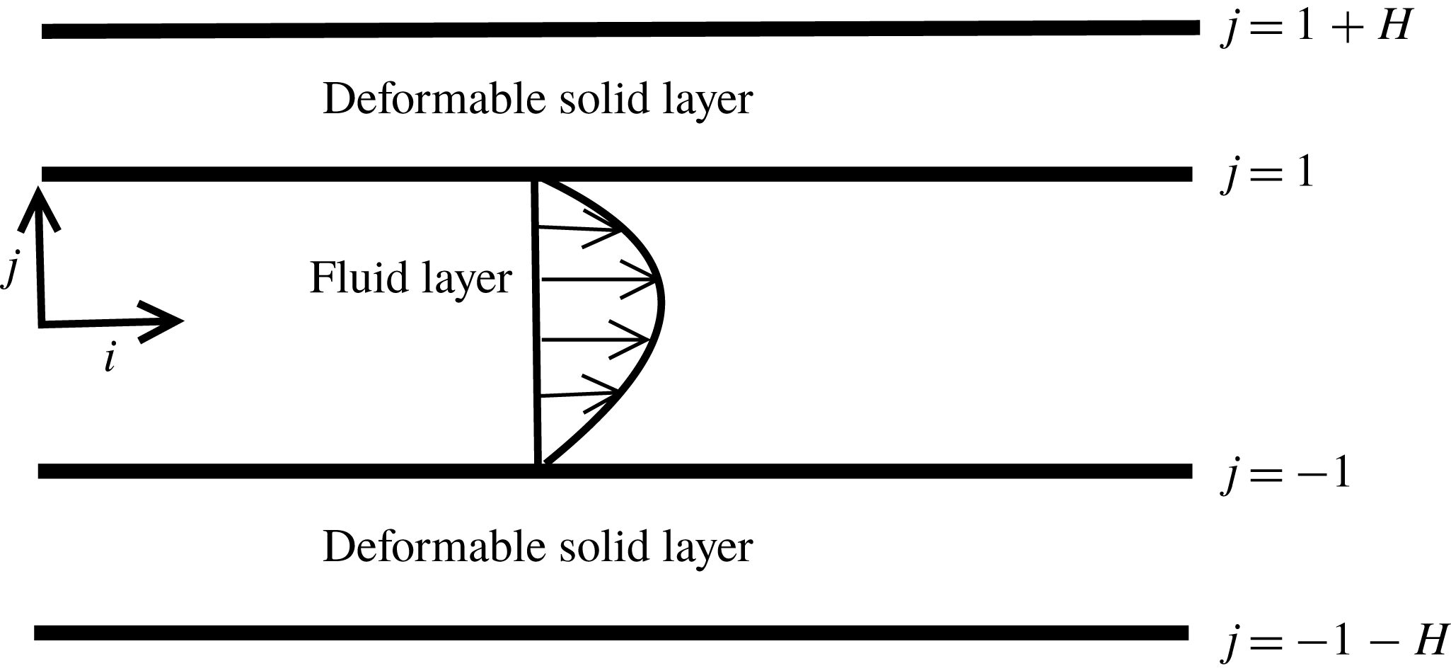
. The schematic of the geometry under consideration is shown in figure 2.
Schematic illustration of pressure-driven flows through deformable channels and tubes. For planar and cylindrical geometries the dimensionless coordinates are respectively
 $i=x$
,
 $j=y$
and
 $i=z$
,
 $j=r$
.

For the fluid, the velocity field is
 $\boldsymbol{v}=(v_{x},v_{y})$
where
 $v_{x}$
and
 $v_{y}$
are respectively the velocities in the
 $x$
and
 $y$
directions. The continuity equation for the fluid is,
 $$\begin{eqnarray}\displaystyle \unicode[STIX]{x1D735}\boldsymbol{\cdot }\boldsymbol{v}=0. & & \displaystyle\end{eqnarray}$$
The dimensionless Navier–Stokes equation is
 $$\begin{eqnarray}\displaystyle Re\left(\frac{\unicode[STIX]{x2202}\boldsymbol{v}}{\unicode[STIX]{x2202}t}+(\boldsymbol{v}\boldsymbol{\cdot }\unicode[STIX]{x1D735})\boldsymbol{v}\right)=-\unicode[STIX]{x1D735}p+\unicode[STIX]{x1D6FB}^{2}\boldsymbol{v}. & & \displaystyle\end{eqnarray}$$
Here,
 $Re=\unicode[STIX]{x1D70C}V_{m}R/\unicode[STIX]{x1D702}$
is the Reynolds number and
 $p$
is the pressure field in the fluid. The fully developed base-state velocity profile is
 $$\begin{eqnarray}\displaystyle \bar{v}_{x}(y)=1-y^{2}, & & \displaystyle\end{eqnarray}$$
where overbar signifies a base-state quantity. For the solid, consider a representative particle with position vector
 $\boldsymbol{X}=(X,Y,Z)$
. We assume an incompressible solid and base-state displacement only in the fluid flow (tangential) direction. With regard to the assumption of incompressibility, the experimental work of Verma & Kumaran (Reference Verma and Kumaran2013) showed that the compression (bulk) modulus
 $K$
of polydimethylsiloxane (PDMS) gel is two orders of magnitude more than the shear modulus
 $G$
. Assuming
 $G/K\sim 0.01$
, we find that Poisson’s ratio is
 $0.485$
, which is very close to
 $0.5$
when the solid is truly incompressible. Thus, it is believed that the incompressibility assumption is fairly accurate in the description of such soft solid materials.
The representative particle, after base-state deformation, now assumes a position vector
 $\bar{\boldsymbol{x}}=(\bar{x},\bar{y},\bar{z})$
such that
 $\bar{\boldsymbol{x}}(\boldsymbol{X})=\boldsymbol{X}+\bar{\boldsymbol{u}}(\boldsymbol{X})$
where
 $\bar{\boldsymbol{u}}(\boldsymbol{X})=(\bar{u}_{x},\bar{u}_{y})(\boldsymbol{X})$
with
 $\bar{u}_{x}(\boldsymbol{X})$
and
 $\bar{u}_{y}(\boldsymbol{X})$
respectively as the base-state Lagrangian displacements in the
 $x$
and
 $y$
directions. For the perturbed state, we track the same representative particle after imposing infinitesimal perturbations on the pre-stressed state. The current position of the particle is
 $\boldsymbol{x}=(x,y,z)$
and related to
 $\bar{\boldsymbol{x}}$
by relation
 $\boldsymbol{x}(\bar{\boldsymbol{x}})=\bar{\boldsymbol{x}}+\boldsymbol{u}^{\prime }(\bar{\boldsymbol{x}},\boldsymbol{t})$
where
 $\boldsymbol{u}^{\prime }(\bar{\boldsymbol{x}},\boldsymbol{t})=(u_{x}^{\prime },u_{y}^{\prime })(\bar{\boldsymbol{x}},t)$
with
 $u_{x}^{\prime }(\bar{\boldsymbol{x}},t)$
and
 $u_{y}^{\prime }(\bar{\boldsymbol{x}},t)$
respectively as the perturbed-state Lagrangian displacements in the
 $x$
and
 $y$
directions.
In nonlinear solid mechanics, the reference state can be any well-defined state of deformation (Holzapfel Reference Holzapfel2000) in the solid for describing the kinematics of the solid deformation. In our problem, it could either be the stress-free base state or the pre-stressed base state of the solid. However, the choice of the stress-free base state as the reference state (Gaurav & Shankar Reference Shankar2010) leads to an ambiguity in the linearisation of interface conditions while performing the linear stability analysis. Hence, in the context of a linear stability analysis, it is more appropriate to use the pre-stressed base state as the reference state in the solid.
To obtain the governing equations we proceed as follows. We consider that the solid is in the current state and the position vector of a representative particle is denoted by
 $\boldsymbol{x}^{\boldsymbol{c}}$
where superscript ‘
 $c$
’ signifies the current state. The solid is further assumed to reach the current state by undergoing a deformation due to the stresses (be it in the base state or with imposed perturbations) exerted by the fluid flowing past it. For the generalisation of the derivation of the momentum balance equations, we consider a representative particle that had position vector
 $\boldsymbol{x}^{\boldsymbol{r}}$
in any arbitrary reference state which the solid underwent before reaching the current state where the superscript ‘
 $r$
’ signifies the reference state. This assumption is valid for any well-behaved motion, i.e. when cracks do not form in the deformable solid while undergoing deformation.
The Cauchy momentum balance equation in the Eulerian (referred to as ‘spatial’ in Holzapfel (Reference Holzapfel2000)) description is
 $$\begin{eqnarray}\displaystyle \unicode[STIX]{x1D70C}\frac{\text{D}\boldsymbol{v}^{\boldsymbol{s}}}{\text{D}t}=\unicode[STIX]{x1D735}_{\boldsymbol{x}^{\boldsymbol{c}}}\boldsymbol{\cdot }\unicode[STIX]{x1D748}, & & \displaystyle\end{eqnarray}$$
here
 $\unicode[STIX]{x1D70C},\boldsymbol{v}^{\boldsymbol{s}},\unicode[STIX]{x1D748}$
and
 $\unicode[STIX]{x1D735}_{\boldsymbol{x}^{\boldsymbol{c}}}$
are respectively the density of the solid, velocity of the representative particle, the Cauchy stress and the gradient operator with the subscript denoting that it acts in spatial coordinates and
 $\text{D}/\text{D}t$
is the substantial derivative. It must be noted that in the above equation the body force terms have been neglected as for the present purpose such forces are absent. Since our definition of the deformation gradient is the transpose of the deformation gradient defined in Holzapfel (Reference Holzapfel2000), to compare equations with the latter, the necessary transformations are
 $\unicode[STIX]{x1D641}_{\boldsymbol{H}}\rightarrow \unicode[STIX]{x1D641}^{\text{T}}$
and
 $\unicode[STIX]{x1D64B}_{\boldsymbol{H}}\rightarrow \unicode[STIX]{x1D64B}^{\text{T}}$
where
 $\unicode[STIX]{x1D64B}$
is the first Piola–Kirchoff stress tensor and subscript
 $H$
signifies the quantities from Holzapfel (Reference Holzapfel2000). The Cauchy and the first Piola–Kirchoff tensors are related as
 $$\begin{eqnarray}\displaystyle \unicode[STIX]{x1D64B}=\unicode[STIX]{x1D641}^{-1}\boldsymbol{\cdot }\unicode[STIX]{x1D748}. & & \displaystyle\end{eqnarray}$$
To obtain the momentum balance equation in the Lagrangian (referred to as ‘material’ in Holzapfel (Reference Holzapfel2000)) description, we convert above equation to the Lagrangian description by using deformation gradient tensors (
 $\unicode[STIX]{x1D641}$
) as follows. Since we have assumed incompressible solid, thus
 $\det (\unicode[STIX]{x1D641})=1$
. The divergence of the first Piola–Kirchoff stress tensor with respect to any arbitrary reference coordinate
 $\boldsymbol{x}^{\boldsymbol{r}}$
is
 $$\begin{eqnarray}\displaystyle \unicode[STIX]{x1D735}_{\boldsymbol{x}^{\boldsymbol{r}}}\boldsymbol{\cdot }\unicode[STIX]{x1D64B}=\unicode[STIX]{x1D735}_{\boldsymbol{x}^{\boldsymbol{r}}}\boldsymbol{\cdot }(\unicode[STIX]{x1D641}^{-1}\boldsymbol{\cdot }\unicode[STIX]{x1D748})=(\unicode[STIX]{x1D735}_{\boldsymbol{x}^{\boldsymbol{r}}}\boldsymbol{\cdot }\unicode[STIX]{x1D641}^{-1})\boldsymbol{\cdot }\unicode[STIX]{x1D748}+\unicode[STIX]{x1D641}^{-1}\boldsymbol{\cdot }(\unicode[STIX]{x1D735}_{\boldsymbol{x}^{\boldsymbol{r}}}\boldsymbol{\cdot }\unicode[STIX]{x1D748})=\unicode[STIX]{x1D641}^{-1}\boldsymbol{\cdot }(\unicode[STIX]{x1D735}_{\boldsymbol{x}^{\boldsymbol{r}}}\boldsymbol{\cdot }\unicode[STIX]{x1D748}), & & \displaystyle\end{eqnarray}$$
where to reach the last step, we have used the Piola identity
 $\unicode[STIX]{x1D735}_{\boldsymbol{x}^{\boldsymbol{r}}}\boldsymbol{\cdot }\unicode[STIX]{x1D641}^{-1}=0$
(Holzapfel (Reference Holzapfel2000), p. 146). Additionally, the deformation gradient that connects any two states of the solid is
 $\unicode[STIX]{x1D641}=\unicode[STIX]{x2202}\boldsymbol{x}^{\boldsymbol{c}}/\unicode[STIX]{x2202}\boldsymbol{x}^{\boldsymbol{r}}$
. To obtain the final equation we use following identity derived by using the chain rule of differentiation
 $$\begin{eqnarray}\displaystyle & \displaystyle \frac{\unicode[STIX]{x2202}\unicode[STIX]{x1D70E}_{ji}}{\unicode[STIX]{x2202}x_{J}^{r}}=\frac{\unicode[STIX]{x2202}x_{j}^{c}}{\unicode[STIX]{x2202}x_{J}^{r}}\frac{\unicode[STIX]{x2202}\unicode[STIX]{x1D70E}_{ji}}{\unicode[STIX]{x2202}x_{j}^{c}}=F_{Jj}\frac{\unicode[STIX]{x2202}\unicode[STIX]{x1D70E}_{ji}}{\unicode[STIX]{x2202}x_{j}^{c}}, & \displaystyle\end{eqnarray}$$
 $$\begin{eqnarray}\displaystyle & \displaystyle \unicode[STIX]{x1D735}_{\boldsymbol{x}^{\boldsymbol{r}}}\boldsymbol{\cdot }\unicode[STIX]{x1D748}=\unicode[STIX]{x1D641}\boldsymbol{\cdot }(\unicode[STIX]{x1D735}_{\boldsymbol{x}^{\boldsymbol{c}}}\boldsymbol{\cdot }\unicode[STIX]{x1D748}), & \displaystyle\end{eqnarray}$$
where the second equation is the vector form of the first equation. Substituting (2.8) in (2.6), we obtain
 $\unicode[STIX]{x1D735}_{\boldsymbol{x}^{\boldsymbol{r}}}\boldsymbol{\cdot }\unicode[STIX]{x1D64B}=\unicode[STIX]{x1D735}_{\boldsymbol{x}^{\boldsymbol{c}}}\boldsymbol{\cdot }\unicode[STIX]{x1D748}$
. Using the preceding relation between
 $\unicode[STIX]{x1D64B}$
and
 $\unicode[STIX]{x1D748}$
in (2.4) along with the recognition that the velocity field is described in the Lagrangian formulation (denoted by
 $\boldsymbol{V}$
, to avoid confusion with
 $\boldsymbol{v}$
, which is reserved to denote the Eulerian fluid velocity) we obtain,
 $$\begin{eqnarray}\displaystyle \unicode[STIX]{x1D70C}\frac{\unicode[STIX]{x2202}\boldsymbol{V}}{\unicode[STIX]{x2202}t}=\unicode[STIX]{x1D735}_{\boldsymbol{x}^{\boldsymbol{r}}}\boldsymbol{\cdot }\unicode[STIX]{x1D64B}. & & \displaystyle\end{eqnarray}$$
For the base-state derivation the reference state is the undeformed state,
 $\boldsymbol{x}^{\boldsymbol{r}}=\boldsymbol{X}$
while the current state is the pre-stressed state such that
 $\boldsymbol{x}^{\boldsymbol{c}}=\bar{\boldsymbol{x}}$
. Thus the deformation gradient becomes
 $\unicode[STIX]{x1D641}=\unicode[STIX]{x2202}\bar{\boldsymbol{x}}/\unicode[STIX]{x2202}\boldsymbol{X}$
which is denoted by
 $\bar{\unicode[STIX]{x1D641}}$
. As explained above, it is convenient to use the pre-stressed state as the reference state while deriving the linearised perturbed-state equations, as this leads to an unambiguous linearisation of the interface conditions (Patne et al.
Reference Patne, Giribabu and Shankar2017). Using the pre-stressed state
 $\boldsymbol{x}^{\boldsymbol{r}}=\bar{\boldsymbol{x}}$
as the reference state, and the perturbed state as the current state
 $\boldsymbol{x}^{\boldsymbol{c}}=\boldsymbol{x}$
, the deformation gradient to transform the Cauchy stress tensor in the perturbed state to the first Piola–Kirchoff stress tensor (based on the pre-stressed reference state) is
 $\unicode[STIX]{x1D641}=\unicode[STIX]{x2202}\boldsymbol{x}/\unicode[STIX]{x2202}\bar{\boldsymbol{x}}$
denoted by
 $\unicode[STIX]{x1D641}^{\prime }$
. Thus the relationship between the Cauchy stress and first Piola–Kirchoff stress tensors for the L3 formulation to derive the perturbed state becomes
 $\unicode[STIX]{x1D64B}=\unicode[STIX]{x1D641}^{\prime -1}\boldsymbol{\cdot }\unicode[STIX]{x1D748}$
, where the pre-stressed base state of the solid is the reference state.
The dimensionless Cauchy stress tensor for purely elastic neo-Hookean solid is (Macosko Reference Macosko1994; Holzapfel Reference Holzapfel2000; Patne et al. Reference Patne, Giribabu and Shankar2017)
 $$\begin{eqnarray}\displaystyle \unicode[STIX]{x1D748}=-p_{g}\unicode[STIX]{x1D644}+\frac{1}{\unicode[STIX]{x1D6E4}}\unicode[STIX]{x1D641}\boldsymbol{\cdot }\unicode[STIX]{x1D641}^{\text{T}}, & & \displaystyle\end{eqnarray}$$
here
 $\unicode[STIX]{x1D6E4}=\unicode[STIX]{x1D702}V_{m}/(GR)$
is the dimensionless base-state velocity. By using the above Cauchy stress tensor and using
 $\boldsymbol{V}=\unicode[STIX]{x2202}\boldsymbol{u}/\unicode[STIX]{x2202}t$
in (2.9), the governing equations for the solid become
 $$\begin{eqnarray}\displaystyle & \displaystyle \det (\unicode[STIX]{x1D641})=1, & \displaystyle\end{eqnarray}$$
 $$\begin{eqnarray}\displaystyle & \displaystyle Re\frac{\unicode[STIX]{x2202}^{2}\boldsymbol{u}}{\unicode[STIX]{x2202}t^{2}}=\unicode[STIX]{x1D735}_{\boldsymbol{x}^{\boldsymbol{r}}}\boldsymbol{\cdot }\unicode[STIX]{x1D64B}. & \displaystyle\end{eqnarray}$$
The governing equations are applicable both in the base state and in the perturbed state. To derive the base state, we use substitution
 $\unicode[STIX]{x1D641}=\bar{\unicode[STIX]{x1D641}}=\unicode[STIX]{x2202}\bar{\boldsymbol{x}}/\unicode[STIX]{x2202}\boldsymbol{X}$
and
 $p_{g}=\bar{p}_{g}$
. It must be noted that the constitutive equation (2.10) is independent of the formulation and has the deformation-free base state as the reference state so as to consider the total strain energy stored in the solid. For the L3 formulation this is accomplished by using relation
 $\unicode[STIX]{x1D641}=\unicode[STIX]{x1D641}^{\prime }\boldsymbol{\cdot }\bar{\unicode[STIX]{x1D641}}$
in (2.10). However, in (2.5), when expressing the first Piola–Kirchoff tensor, we use
 $\unicode[STIX]{x1D641}^{\prime }$
to transform the Cauchy stress to the pre-stressed reference state. Additionally, for the perturbed state
 $p_{g}=\bar{p}_{g}+p_{g}^{\prime }$
where
 $p_{g}^{\prime }$
is the perturbed-state pressure in the solid. Thus the L3 formulation involves change in only the kinematic aspects of the formulation without affecting the fundamental relations in the deformable solid. Following the procedure outlined by Patne et al. (Reference Patne, Giribabu and Shankar2017), the base-state deformation and pressure in the solid, in terms of the pre-stressed-state coordinates are
 $$\begin{eqnarray}\displaystyle \bar{u}_{x}(\bar{y})=\unicode[STIX]{x1D6E4}((1+H)^{2}-\bar{y}^{2}),\quad \bar{u}_{y}(\bar{y})=0;\quad \bar{p}_{g}(\bar{x})=-2\bar{x}. & & \displaystyle\end{eqnarray}$$
As Squire’s theorem is not applicable for the current system, we must consider three-dimensional disturbances. However, in § 3.3 we numerically show three-dimensional disturbances to be more stable than corresponding two-dimensional disturbances for flows past deformable surfaces provided that a consistent formulation is used. Consequently here we assume two-dimensional disturbances and use normal modes of the form
 $$\begin{eqnarray}\displaystyle & \displaystyle (v_{x}^{\prime },v_{y}^{\prime },p^{\prime })(\boldsymbol{x},t)=(\tilde{v}_{x},\tilde{v}_{y},\tilde{p})(y)\text{e}^{\text{i}k(x-ct)}, & \displaystyle\end{eqnarray}$$
 $$\begin{eqnarray}\displaystyle & \displaystyle (u_{x}^{\prime },u_{y}^{\prime },p_{g}^{\prime })(\bar{\boldsymbol{x}},t)=(\tilde{u} _{x},\tilde{u} _{y},\tilde{p}_{g})(\bar{y})\text{e}^{\text{i}k(\bar{x}-ct)}, & \displaystyle\end{eqnarray}$$
where,
 $k$
is the wavenumber in the
 $x$
or
 $\bar{x}$
direction and only takes real values. The complex wave speed of the perturbations is
 $c=c_{r}+\text{i}c_{i}$
and the base flow is unstable if at least one eigenvalue satisfies the condition
 $c_{i}>0$
. The linearised governing equations for perturbations in the fluid after using the above normal modes are
 $$\begin{eqnarray}\displaystyle & \displaystyle \text{i}k\tilde{v}_{x}+D\tilde{v}_{y}=0, & \displaystyle\end{eqnarray}$$
 $$\begin{eqnarray}\displaystyle & \displaystyle -\text{i}k\tilde{p}+(D^{2}-k^{2})\tilde{v}_{x}=Re[\text{i}k\tilde{v}_{x}(\bar{v}_{x}-c)+D\bar{v}_{x}\tilde{v}_{y}], & \displaystyle\end{eqnarray}$$
 $$\begin{eqnarray}\displaystyle & \displaystyle -D\tilde{p}+(D^{2}-k^{2})\tilde{v}_{y}=Re[\text{i}k\tilde{v}_{y}(\bar{v}_{x}-c)], & \displaystyle\end{eqnarray}$$
where,
 $D=\text{d}/\text{d}y$
. Similarly, for the solid, the linearised governing equations are
 $$\begin{eqnarray}\displaystyle & \displaystyle \text{i}k\tilde{u} _{x}+D\tilde{u} _{y}=0, & \displaystyle\end{eqnarray}$$
 $$\begin{eqnarray}\displaystyle & \displaystyle -\text{i}k\tilde{p}_{g}+\frac{1}{\unicode[STIX]{x1D6E4}}(D^{2}+2\text{i}kD\bar{u}_{x}D-k^{2}(1+(D\bar{u}_{x})^{2})+\text{i}kD^{2}\bar{u}_{x})\tilde{u} _{x}-D_{\bar{x}}\bar{p}_{g}D\tilde{u} _{y}=-k^{2}c^{2}Re\tilde{u} _{x}, & \displaystyle \nonumber\\ \displaystyle & & \displaystyle\end{eqnarray}$$
 $$\begin{eqnarray}\displaystyle & \displaystyle -D\tilde{p}_{g}+\frac{1}{\unicode[STIX]{x1D6E4}}(D^{2}+2\text{i}kD\bar{u}_{x}D-k^{2}(1+(D\bar{u}_{x})^{2})+\text{i}kD^{2}\bar{u}_{x})\tilde{u} _{y}+D_{\bar{x}}\bar{p}_{g}D\tilde{u} _{x}=-k^{2}c^{2}Re\tilde{u} _{y}, & \displaystyle \nonumber\\ \displaystyle & & \displaystyle\end{eqnarray}$$
where
 $D=\text{d}/\text{d}\bar{y}$
and
 $D_{\bar{x}}=\text{d}/\text{d}\bar{x}$
. The linearised perturbation equations for the fluid and solid are then solved by using following boundary conditions.
For plane Poiseuille flow through a rectangular rigid channel, following Drazin & Howard (Reference Drazin, Howard and Chernyi1966), the disturbances can be classified into two types, viz., varicose (odd) and sinuous (even) modes depending on the symmetry of the streamwise velocity perturbation eigenfunctions about the channel centre. In our deformable neo-Hookean channel, both the deformable layers are of identical thickness and shear modulus, and hence the disturbance can be divided into sinuous and varicose modes. If we combine the spectra obtained for varicose and sinuous modes, this will result in the full spectrum obtained by considering three-layered structure with fluid layer sandwiched between the neo-Hookean layers as shown in figure 2. This mode separation (into sinuous and varicose) is also carried out to facilitate comparison with the earlier work of Gkanis & Kumar (Reference Gkanis and Kumar2005) who studied only varicose modes. Thus, at the centre of the channel (
 $y=0$
) the following boundary conditions are applicable (Drazin & Howard Reference Drazin, Howard and Chernyi1966)
 $$\begin{eqnarray}\displaystyle & \displaystyle \tilde{v}_{y}=0;D\tilde{v}_{x}=0,\quad \text{varicose or odd modes}, & \displaystyle\end{eqnarray}$$
 $$\begin{eqnarray}\displaystyle & \displaystyle \tilde{v}_{x}=0;D^{2}\tilde{v}_{x}=0,\quad \text{sinuous or even modes}. & \displaystyle\end{eqnarray}$$
The varicose (odd) and sinuous (even) modes are respectively the modes for which
 $v_{y}$
is an odd or even function of
 $y$
. At
 $y=1$
, i.e. at the fluid–soft solid interface, velocity and stress continuity give
 $$\begin{eqnarray}\displaystyle & \displaystyle \tilde{v}_{y}=-\text{i}kc\tilde{u} _{y}, & \displaystyle\end{eqnarray}$$
 $$\begin{eqnarray}\displaystyle & \displaystyle \tilde{v}_{x}+(D\bar{v}_{x})|_{y=1}\tilde{u} _{y}=-\text{i}kc\tilde{u} _{x}, & \displaystyle\end{eqnarray}$$
 $$\begin{eqnarray}\displaystyle & \displaystyle \frac{1}{\unicode[STIX]{x1D6E4}}(D\tilde{u} _{x}+\text{i}k\tilde{u} _{y})=D\tilde{v}_{x}+\text{i}k\tilde{v}_{y}+(D^{2}\bar{v}_{x})|_{y=1}\tilde{u} _{y}, & \displaystyle\end{eqnarray}$$
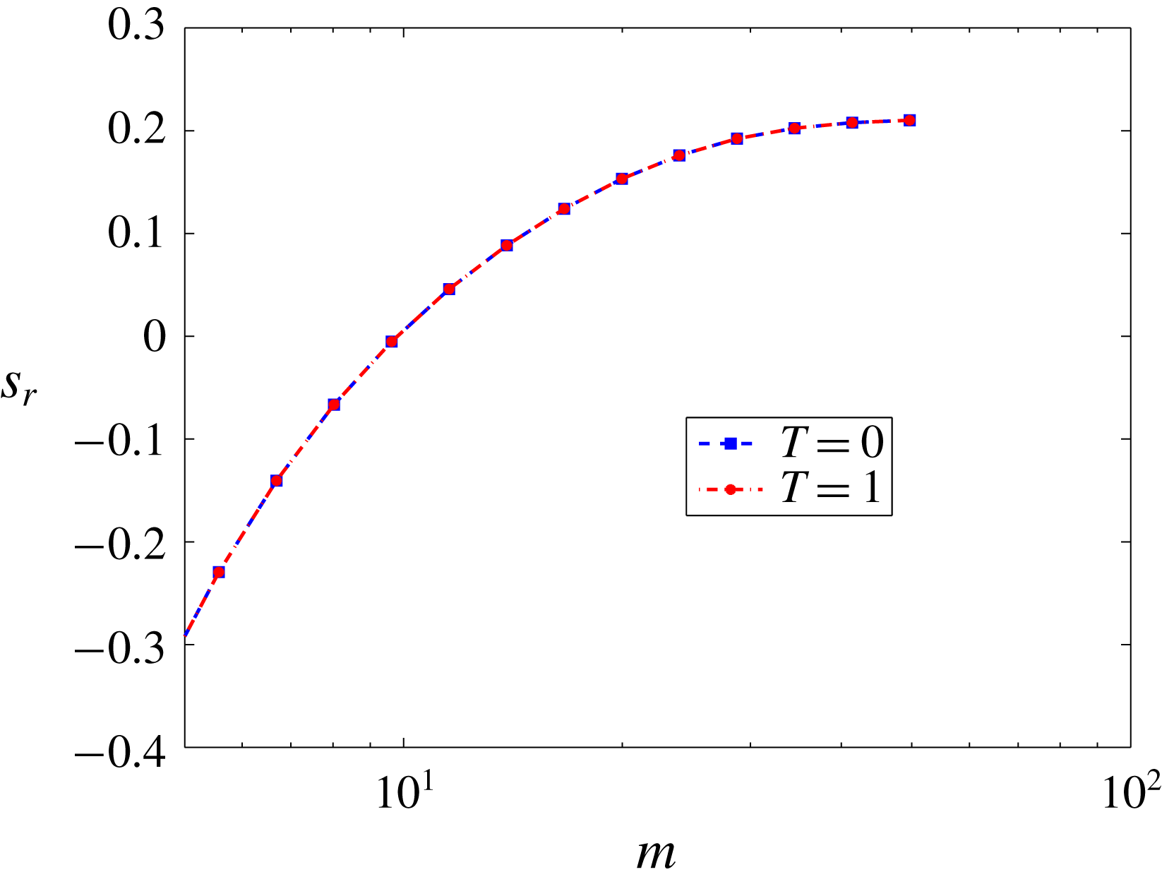
 $$\begin{eqnarray}\displaystyle & \displaystyle -\tilde{p}_{g}+\frac{2}{\unicode[STIX]{x1D6E4}}(\text{i}k(D\bar{u}_{x})|_{\bar{y}=1}+D)\tilde{u} _{y}=-\tilde{p}+2D\tilde{v}_{y}-\text{}\underline{(D_{x}\bar{p})|_{y=1}\tilde{u} _{x}}-\frac{T}{\unicode[STIX]{x1D6E4}}k^{2}\tilde{u} _{y}, & \displaystyle\end{eqnarray}$$
here
 $T=\unicode[STIX]{x1D6F4}/(GR)$
is the dimensionless fluid–solid interface tension with
 $\unicode[STIX]{x1D6F4}$
as the dimensional interface tension and
 $(D\bar{u}_{x})|_{\bar{y}=1}$
denotes evaluation of
 $D\bar{u}_{x}$
at
 $\bar{y}=1$
. The underlined term in the last equation arises because of the Taylor series expansion of the base-state fluid quantities in the flow direction which was absent in the previous studies. This extra term represents the effect of the base-state pressure gradient on the energy exchange between the base state and perturbations at the fluid–deformable solid interface, which is shown to play a very important role in the stability behaviour of the system, as discussed in § 3.1. At
 $\bar{y}=1+H$
, we assume perfect bonding between deformable and rigid solids, hence
 $$\begin{eqnarray}\displaystyle \tilde{\boldsymbol{u}}=0. & & \displaystyle\end{eqnarray}$$
The above equations and boundary conditions are quite general (i.e. they are applicable even when the velocity profiles are non-parabolic) and can be used for any planar flow geometry provided that the pre-stressed-state quantities are known. The above equations and boundary conditions are then solved for the eigenvalue
 $c$
using both numerical integration combined with shooting and pseudo-spectral (Weideman & Reddy Reference Weideman and Reddy2000; Boyd Reference Boyd2001) methods, as explained below.
In the pseudo-spectral method we expand the quantities in terms of the Chebyshev polynomials as
 $\tilde{f}(y)=\sum _{n=0}^{n=N}a_{n}T_{n}(y)$
where
 $\tilde{f}(y),n,N,a_{n}$
and
 $T_{n}(y)$
are respectively the fluid or solid quantity, number of the Chebyshev polynomial, highest degree of the polynomial in the series expansion or the number of the collocation points, coefficient of the
 $n$
th Chebyshev polynomial and
 $n$
th Chebyshev polynomial. Thus we need to evaluate the series expansion at
 $N$
collocation points to evaluate the series coefficients
 $a_{n}$
and/or to obtain the eigenvalue
 $c$
. The discretised matrices then form the matrix problem of the following form
 $$\begin{eqnarray}\displaystyle c^{2}\unicode[STIX]{x1D63E}\boldsymbol{e}+c\unicode[STIX]{x1D63D}\boldsymbol{e}+\unicode[STIX]{x1D63C}\boldsymbol{e}=0, & & \displaystyle\end{eqnarray}$$
where
 $\unicode[STIX]{x1D63C},\unicode[STIX]{x1D63D}$
and
 $\unicode[STIX]{x1D63E}$
are the discretised matrices and
 $\boldsymbol{e}$
is the eigenvector. To solve the above eigenvalue problem, we use the polyeig MATLAB routine. Since the predicted spectrum includes spurious modes, to remove those, the code is executed for
 $N$
and
 $N+2$
numbers of collocation points and then setting the tolerance for the error in predicting the eigenvalues of
 $O(10^{-5})$
. To validate the genuine character of the eigenvalues we change the number of collocation points by
 $25$
and the eigenvalues which remained invariant up to sixth decimal place were then given as an initial guess to the shooting code.
In the shooting code, the fluid governing equations are integrated from the centre of the channel (
 $y=0$
) to the fluid–solid interface (
 $y=1$
) while the deformable solid governing equations are integrated from
 $y=1+H$
to the fluid–solid interface. At the interface we form a matrix by using the interface conditions of order
 $4\times 4$
whose real and imaginary parts of the determinant must vanish separately for a genuine eigenvalue. To integrate the fluid and solid governing equations we use the built-in routine ode45 of MATLAB. If the shooting code converges to the eigenvalue after a finite number of iterations (usually 10–20 iterations), then it is regarded as a genuine eigenvalue.
2.3 Hagen–Poiseuille flow through a Mooney–Rivlin tube
The procedure followed here is similar to the one used for Hagen–Poiseuille flow through a neo-Hookean tube using the L3 formulation by Patne et al. (Reference Patne, Giribabu and Shankar2017), except for the Cauchy stress tensor. We consider an incompressible Newtonian fluid flowing through a tube of radius
 $R_{t}$
in the undeformed state and deformable walls from
 $r=R_{t}$
to
 $r=R_{t}(1+H)$
as shown in figure 2. The lengths, velocity and pressure are respectively non-dimensionalised by
 $R_{t}$
,
 $(2C_{1}R_{t})/\unicode[STIX]{x1D702}$
and
 $2C_{1}$
. For a Mooney–Rivlin solid in the limit of infinitesimally small deformations the shear modulus is
 $G\approx 2(C_{1}+C_{2})$
hence the pressure should be non-dimensionalised by
 $2(C_{1}+C_{2})$
and not
 $2C_{1}$
. However, to compare with the neo-Hookean model and for the ease of formulation we use
 $2C_{1}$
in place of
 $2(C_{1}+C_{2})$
. In the results section, we redefine the non-dimensional parameters to accommodate the shear modulus definition for the Mooney–Rivlin solid.
In the following discussion, for the sake of brevity, the non-dimensional dynamical variables are denoted without any subscript or superscript. The continuity and momentum balance equations for the fluid reduce to (2.1) and (2.2) with Reynolds number,
 $Re=\unicode[STIX]{x1D70C}R_{t}V_{t}/\unicode[STIX]{x1D702}$
and dimensionless maximum velocity in the base state,
 $\unicode[STIX]{x1D6FE}=\unicode[STIX]{x1D702}V_{t}/(2C_{1}R_{t})$
. Assuming an axisymmetric velocity field for the fluid,
 $\boldsymbol{v}=(v_{r},v_{z})$
where
 $v_{r}$
and
 $v_{z}$
are respectively the velocity components in the
 $r$
and
 $z$
directions, the base-state velocity profile is that of a fully developed pressure-driven Hagen–Poiseuille flow in the tube
 $$\begin{eqnarray}\displaystyle \bar{v}_{z}(r)=\unicode[STIX]{x1D6FE}(1-r^{2}). & & \displaystyle\end{eqnarray}$$
The dimensionless Cauchy stress tensor for the Mooney–Rivlin model in Lagrangian formulation (third row and first column of table 2) is
 $$\begin{eqnarray}\displaystyle \unicode[STIX]{x1D748}=-p_{g}\unicode[STIX]{x1D644}+(\unicode[STIX]{x1D641}\boldsymbol{\cdot }\unicode[STIX]{x1D641}^{\text{T}})-\unicode[STIX]{x1D6FD}(\unicode[STIX]{x1D641}\boldsymbol{\cdot }\unicode[STIX]{x1D641}^{\text{T}})^{-1}, & & \displaystyle\end{eqnarray}$$
where
 $\unicode[STIX]{x1D6FD}=C_{2}/C_{1}$
. For realistic deformable solid materials,
 $0<\unicode[STIX]{x1D6FD}<1$
(Macosko Reference Macosko1994; Holzapfel Reference Holzapfel2000). For the base state, using substitution
 $\unicode[STIX]{x1D641}=\bar{\unicode[STIX]{x1D641}}$
in the above equation and following the procedure outlined for Hagen–Poiseuille flow through a neo-Hookean tube by Patne et al. (Reference Patne, Giribabu and Shankar2017) and using (2.12), we obtain
 $$\begin{eqnarray}\displaystyle & \displaystyle \bar{u}_{z}(\bar{r})=\frac{\unicode[STIX]{x1D6FE}}{(1+\unicode[STIX]{x1D6FD})}[(1+H)^{2}-\bar{r}^{2}];\quad \bar{u}_{r}(\bar{r})=0, & \displaystyle\end{eqnarray}$$
 $$\begin{eqnarray}\displaystyle & \displaystyle \bar{p}_{g}(\bar{r},\bar{z})=-4\unicode[STIX]{x1D6FE}\bar{z}+\frac{6\unicode[STIX]{x1D6FE}^{2}\unicode[STIX]{x1D6FD}}{(1+\unicode[STIX]{x1D6FD})^{2}}((1+H)^{2}-\bar{r}^{2}), & \displaystyle\end{eqnarray}$$
where
 $\bar{u}_{z}(\bar{r})$
and
 $\bar{u}_{r}(\bar{r})$
are respectively the base-state Lagrangian deformations of the solid in the
 $z$
and
 $r$
directions. For a neo-Hookean solid
 $\bar{p}_{g}(\bar{r},\bar{z})$
is a function of
 $\bar{z}$
alone while for a Mooney–Rivlin solid it is a function of both
 $\bar{r}$
and
 $\bar{z}$
because of the presence of
 $\boldsymbol{b}^{-1}$
term which is analogous to the Eulerian (CK) formulation for which
 $\bar{p}_{g}(\bar{r},\bar{z})$
was also a function of
 $\bar{r}$
and
 $\bar{z}$
(Patne et al.
Reference Patne, Giribabu and Shankar2017). Next we impose infinitesimally small axisymmetric perturbations and linearise the equations. In the linearised equations we then substitute the normal modes
 $$\begin{eqnarray}\displaystyle & \displaystyle (v_{r}^{\prime },v_{z}^{\prime },p^{\prime })(\boldsymbol{x},t)=(\text{i}\tilde{v}_{r},\tilde{v}_{z},\tilde{p})(r)\text{e}^{\text{i}k(z-ct)}, & \displaystyle\end{eqnarray}$$
 $$\begin{eqnarray}\displaystyle & \displaystyle (u_{r}^{\prime },u_{z}^{\prime },p_{g}^{\prime })(\bar{\boldsymbol{x}},t)=(\text{i}\tilde{u} _{r},\tilde{u} _{z},\tilde{p}_{g})(\bar{r})\text{e}^{\text{i}k(\bar{z}-ct)}, & \displaystyle\end{eqnarray}$$
where
 $k$
is the wavenumber in the axial (
 $z$
or
 $\bar{z}$
) direction while
 $u_{z}^{\prime }$
and
 $u_{r}^{\prime }$
are respectively the perturbation displacements of the solid in the
 $z$
and
 $r$
directions. The linearised perturbation governing equations for the fluid using (2.1), (2.2) and (2.34) are
 $$\begin{eqnarray}\displaystyle & \displaystyle k\tilde{v}_{z}+\frac{\tilde{v}_{r}}{r}+D\tilde{v}_{r}=0, & \displaystyle\end{eqnarray}$$
 $$\begin{eqnarray}\displaystyle & \displaystyle -D\tilde{p}+\text{i}\left(D^{2}+\frac{1}{r}D-\frac{1}{r^{2}}-k^{2}\right)\tilde{v}_{r}=-\frac{Re}{\unicode[STIX]{x1D6FE}}[k\tilde{v}_{r}(\bar{v}_{z}-c)], & \displaystyle\end{eqnarray}$$
 $$\begin{eqnarray}\displaystyle & \displaystyle -\text{i}k\tilde{p}+\left(D^{2}+\frac{1}{r}D-k^{2}\right)\tilde{v}_{z}=\text{i}\frac{Re}{\unicode[STIX]{x1D6FE}}[k\tilde{v}_{z}(\bar{v}_{z}-c)+D\bar{v}_{z}\tilde{v}_{r}], & \displaystyle\end{eqnarray}$$
where
 $D=\text{d}/\text{d}r$
. Similarly, for the solid, the incompressibility condition for the perturbed state using (2.11) becomes
 $$\begin{eqnarray}\displaystyle k\tilde{u} _{z}+\frac{\tilde{u} _{r}}{\bar{r}}+D\tilde{u} _{r}=0. & & \displaystyle\end{eqnarray}$$
To obtain the linearised momentum balance equations for the solid the substitution
 $\unicode[STIX]{x1D641}=\unicode[STIX]{x1D641}^{\prime }\boldsymbol{\cdot }\bar{\unicode[STIX]{x1D641}}$
is used in (2.31) and the resulting
 $\unicode[STIX]{x1D748}$
is then substituted in (2.12). The resulting linearised equations after substitution of the normal modes (2.35) become,
 $$\begin{eqnarray}\displaystyle & & \displaystyle -\text{i}kp_{g}+\left(D^{2}+\frac{1}{\bar{r}}D-k^{2}\right)\tilde{u} _{z}-\left(\frac{\text{i}}{\bar{r}}D_{z}\bar{p}_{g}+\text{i}D_{z}\bar{p}_{g}D-kD\bar{p}_{g}\right)\tilde{u} _{r}\nonumber\\ \displaystyle & & \displaystyle \quad +\,\left(\text{i}kD^{2}\bar{u}_{z}+2\text{i}kD\bar{u}_{z}D-k^{2}(D\bar{u}_{z})^{2}+\frac{\text{i}k}{\bar{r}}D\bar{u}_{z}D\right)\tilde{u} _{z}\nonumber\\ \displaystyle & & \displaystyle \quad +\,\unicode[STIX]{x1D6FD}\left(D^{2}+\frac{1}{\bar{r}}D+2\text{i}kD^{2}\bar{u}_{z}+\text{i}kD\bar{u}_{z}D+\frac{2\text{i}k}{\bar{r}}D\bar{u}_{z}\right)\tilde{u} _{z}\nonumber\\ \displaystyle & & \displaystyle \quad +\,\unicode[STIX]{x1D6FD}\left(\text{i}D\bar{u}_{z}D^{2}+\text{i}D^{2}\bar{u}_{z}D-k(D\bar{u}_{z})^{2}D+\frac{4\text{i}}{\bar{r}}D\bar{u}_{z}D+kD-2kD\bar{u}_{z}D^{2}\bar{u}_{z}\right)\tilde{u} _{r}\nonumber\\ \displaystyle & & \displaystyle \quad +\,\unicode[STIX]{x1D6FD}\left(\frac{3\text{i}}{\bar{r}}D^{2}\bar{u}_{z}-\frac{k}{\bar{r}}(D\bar{u}_{z})^{2}+2\text{i}k^{2}D\bar{u}_{z}+\frac{k}{\bar{r}}\right)\tilde{u} _{r}=-k^{2}c^{2}\frac{Re}{\unicode[STIX]{x1D6FE}}\tilde{u} _{z},\end{eqnarray}$$
 $$\begin{eqnarray}\displaystyle & & \displaystyle -D\tilde{p}_{g}+\text{i}\left(D^{2}+\frac{1}{\bar{r}}D-\frac{1}{\bar{r}^{2}}-k^{2}\right)\tilde{u} _{r}-(-D_{z}\bar{p}_{g}D+\text{i}kD\bar{p}_{g})\tilde{u} _{z}\nonumber\\ \displaystyle & & \displaystyle \quad -\,\left(kD^{2}\bar{u}_{z}+2kD\bar{u}_{z}D+\text{i}k^{2}(D\bar{u}_{z})^{2}+\frac{k}{\bar{r}}D\bar{u}_{z}D+\frac{i}{\bar{r}}D\bar{p}_{g}\right)\tilde{u} _{r}\nonumber\\ \displaystyle & & \displaystyle \quad -\,\unicode[STIX]{x1D6FD}\left(2D\bar{u}_{z}D^{2}+2D^{2}\bar{u}_{z}D+2\text{i}k(D\bar{u}_{z})^{2}D+\frac{2}{\bar{r}}D\bar{u}_{z}D+\text{i}kD\right)\tilde{u} _{z}\nonumber\\ \displaystyle & & \displaystyle \quad -\,\unicode[STIX]{x1D6FD}\left(6\text{i}kD\bar{u}_{z}D^{2}\bar{u}_{z}+\frac{3\text{i}k}{\bar{r}}(D\bar{u}_{z})^{2}+k^{2}D\bar{u}_{z}\right)\tilde{u} _{z}\nonumber\\ \displaystyle & & \displaystyle \quad -\,\unicode[STIX]{x1D6FD}\left(\frac{3\text{i}}{\bar{r}}(D\bar{u}_{z})^{2}D+kD\bar{u}_{z}D+\frac{6\text{i}}{\bar{r}}D\bar{u}_{z}D^{2}\bar{u}_{z}\right)\tilde{u} _{r}\nonumber\\ \displaystyle & & \displaystyle \quad -\,\unicode[STIX]{x1D6FD}\left(-kD^{2}\bar{u}_{z}+\text{i}k^{2}(D\bar{u}_{z})^{2}+\frac{2k}{\bar{r}}D\bar{u}_{z}+\text{i}k^{2}\right)\tilde{u} _{r}=-k^{2}c^{2}\frac{Re}{\unicode[STIX]{x1D6FE}}\tilde{u} _{r},\end{eqnarray}$$
where
 $D=\text{d}/\text{d}\bar{r}$
and
 $D_{z}=\text{d}/\text{d}\bar{z}$
. The above governing equations reduce to Hagen–Poiseuille flow through a neo-Hookean tube if
 $\unicode[STIX]{x1D6FD}=0$
and
 $C_{1}=G/2$
. To solve these equations the following boundary conditions are used. At
 $r=0$
, the following symmetry conditions are applicable (Batchelor & Gill Reference Batchelor and Gill1962)
 $$\begin{eqnarray}\displaystyle \tilde{v}_{r}=0,\quad D\tilde{v}_{z}=0. & & \displaystyle\end{eqnarray}$$
At
 $r=1$
, i.e. at the fluid–solid interface, by following the procedure developed by Patne et al. (Reference Patne, Giribabu and Shankar2017), we obtain the following linearised interface conditions
 $$\begin{eqnarray}\displaystyle & \displaystyle \tilde{v}_{r}=-\text{i}kc\tilde{u} _{r}, & \displaystyle\end{eqnarray}$$
 $$\begin{eqnarray}\displaystyle & \displaystyle \tilde{v}_{z}+(D\bar{v}_{z})|_{r=1}\tilde{u} _{r}=-\text{i}kc\tilde{u} _{z}, & \displaystyle\end{eqnarray}$$
 $$\begin{eqnarray}\displaystyle & & \displaystyle 2\text{i}k(1+\unicode[STIX]{x1D6FD})(D\bar{u}_{z})|_{\bar{r}=1}\tilde{u} _{z}+2\text{i}(D\bar{u}_{z})|_{\bar{r}=1}D\tilde{u} _{r}\nonumber\\ \displaystyle & & \displaystyle \quad +\,2\text{i}\unicode[STIX]{x1D6E4}\tilde{u} _{r}+2\text{i}\unicode[STIX]{x1D6FD}(D\bar{u}_{z})|_{\bar{r}=1}\tilde{u} _{r}+(1+\unicode[STIX]{x1D6FD})(D\tilde{u} _{z}-k\tilde{u} _{r})=D\tilde{v}_{z}-k\tilde{v}_{r},\end{eqnarray}$$
 $$\begin{eqnarray}\displaystyle & & \displaystyle \quad -\tilde{p}_{g}-2\text{i}\unicode[STIX]{x1D6FD}(1+((D\bar{u}_{z})^{2})|_{\bar{r}=1})(\tilde{u} _{r}+k\tilde{u} _{z})-2\unicode[STIX]{x1D6FD}(D\bar{u}_{z})|_{\bar{r}=1}D\tilde{u} _{z}+2\text{i}D\tilde{u} _{r}\nonumber\\ \displaystyle & & \displaystyle \quad -\,2k(D\bar{u}_{z})|_{\bar{r}=1}\tilde{u} _{r}+(D_{z}\bar{p}_{g})|_{\bar{r}=1}\tilde{u} _{z}+(D\bar{p}_{g})|_{\bar{r}=1}\tilde{u} _{r}=-\tilde{p}+2\text{i}D\tilde{v}_{r}.\end{eqnarray}$$
At
 $y=1+H$
, the boundary condition (2.28) is applicable. The numerical methods used to solve the eigenvalue problem are the same as the ones described in the preceding section.
3 Results and discussion
3.1 Plane Poiseuille flow through a neo-Hookean channel
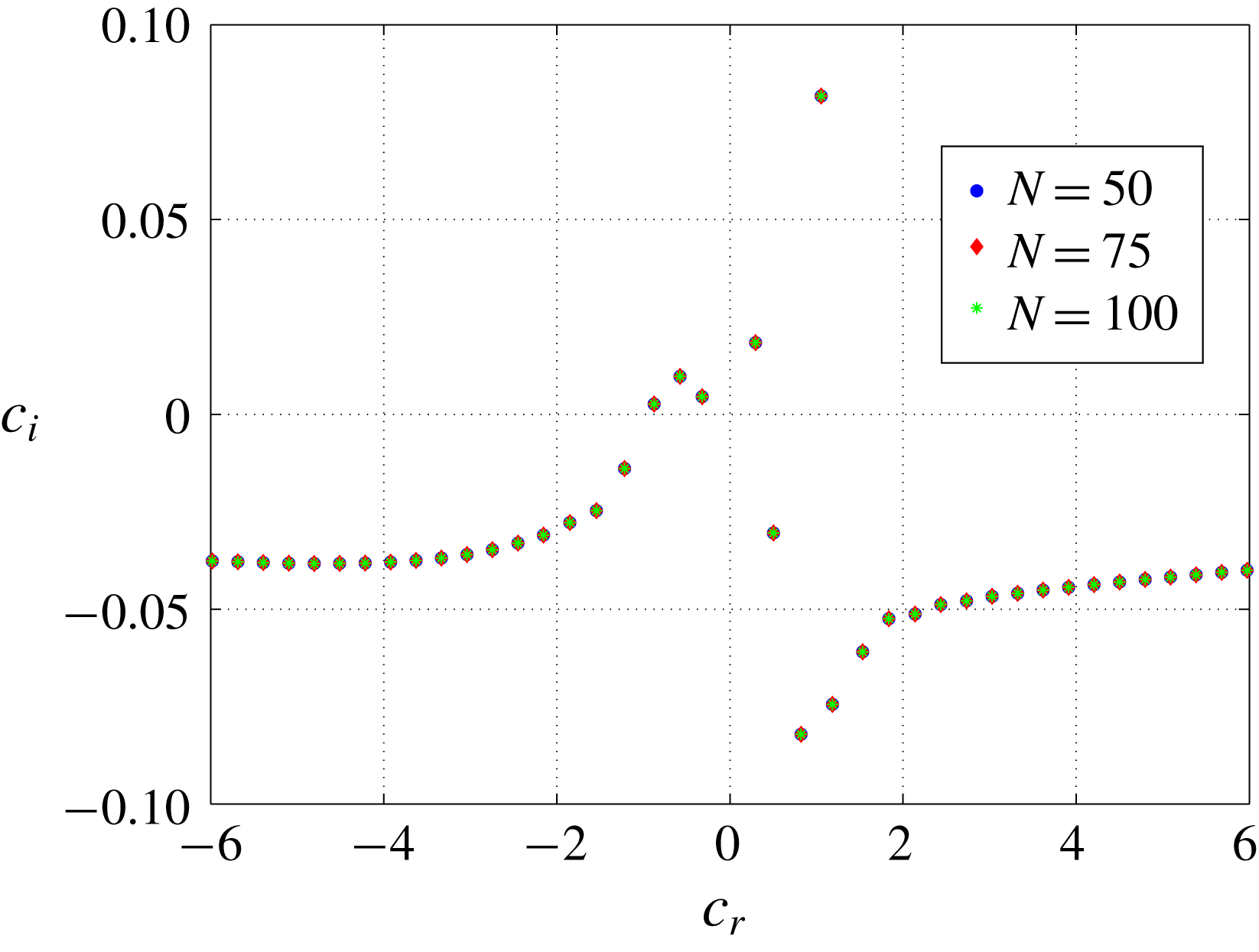
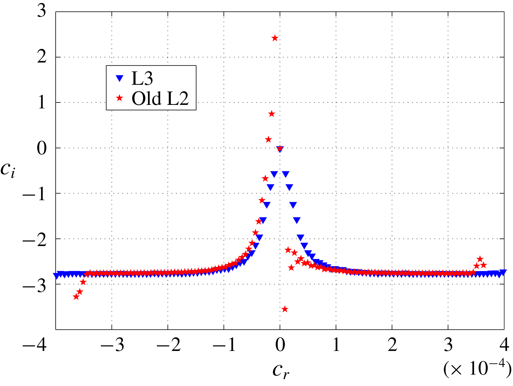
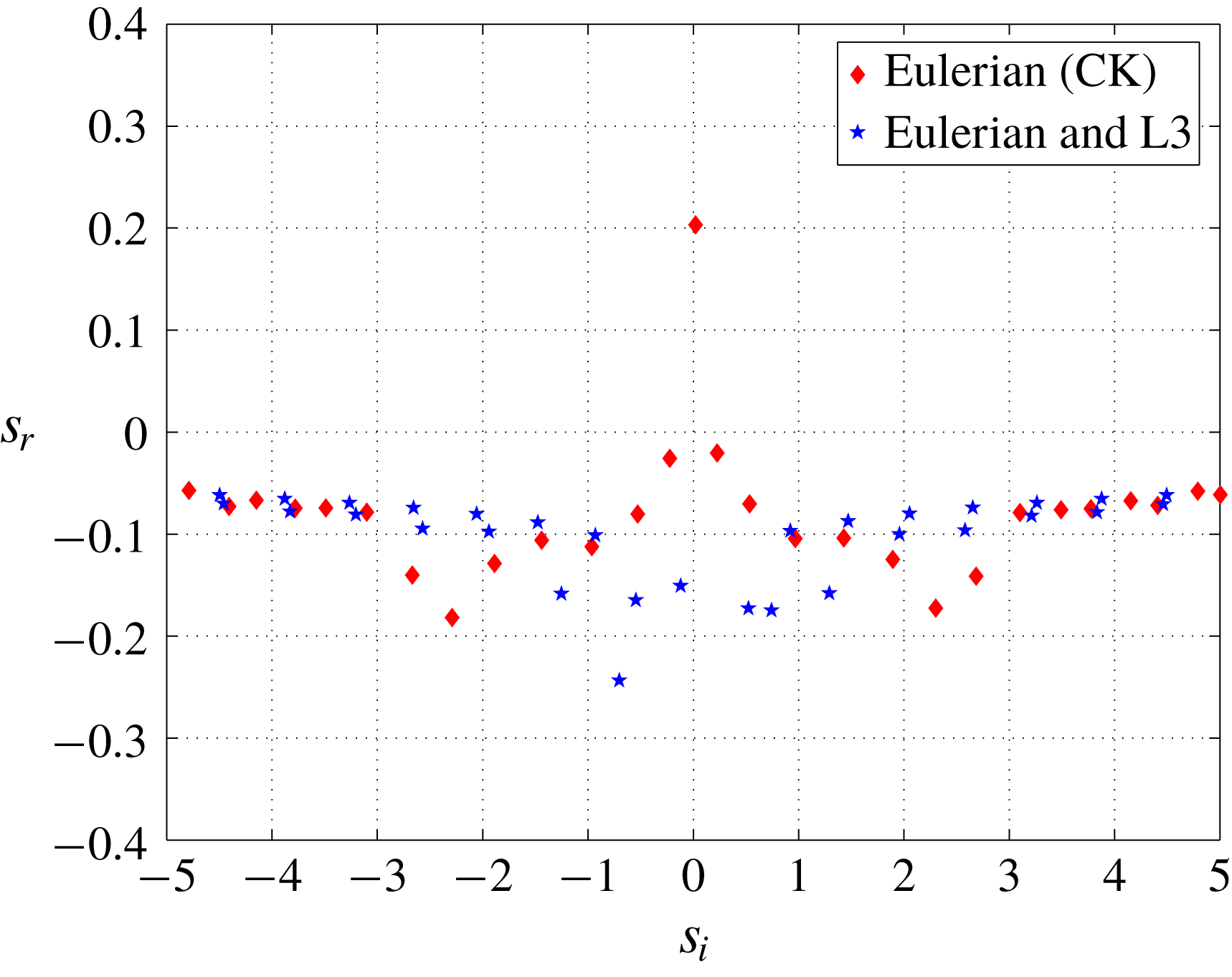
In this section, we compare the results predicted by the old L2 (Gaurav & Shankar Reference Shankar2010) and L3 formulations. Following Gaurav & Shankar (Reference Shankar2010), the stability analysis of the problem is divided into varicose and sinuous modes. Before proceeding with the analysis, we first demonstrate the appropriate number of collocation points required for the convergence of genuine eigenvalues. In figure 3, we plot the spectra for plane Poiseuille flow through a neo-Hookean channel for different numbers of collocation points. We observe that even at
 $N=50$
, the unstable eigenvalues (which determine the stability of the system) are captured and a further increase in the number of collocation points by
 $25$
changes the eigenvalues only at the sixth decimal place. Thus
 $N=50$
is sufficient to study the stability of the system for the parameter ranges explored in this study.
The spectra of plane Poiseuille flow through a neo-Hookean channel at
 $Re=50,k=0.3,\unicode[STIX]{x1D6E4}=1,T=0$
and
 $H=5$
for varying number of collocation points. The convergence of the unstable modes shows the genuine character of the eigenvalues.

3.1.1 Creeping-flow limit
In the creeping-flow limit, plane Couette flow past a deformable solid exhibits a finite-wave instability at the fluid–solid interface when the parameter
 $\unicode[STIX]{x1D6E4}$
exceeds an
 $O(1)$
critical value. This finite-wave instability is very robust, is present in both linear elastic and neo-Hookean models and has been observed in experiments as well (Kumaran & Muralikrishnan Reference Kumaran and Muralikrishnan2000). Fortuitously, the results for plane Couette flow subjected to two-dimensional disturbances are rather insensitive to the various formulations (whether consistent or not), and hence the consistent formulation still predicts the instability of Kumaran & Muralikrishnan (Reference Kumaran and Muralikrishnan2000). (To discern differences between the formulations, as we demonstrate in § 3.3, it is necessary to impose three-dimensional perturbations.) A similar finite-wave instability is predicted to be present in pressure-driven flow through a deformable tube modelled as a linear elastic solid (Kumaran Reference Kumaran1995b
). However, upon the use of a neo-Hookean model, this finite-wave instability is no longer present for flow in a deformable tube and only the short-wave instability is predicted to exist (Gaurav & Shankar Reference Shankar2009).
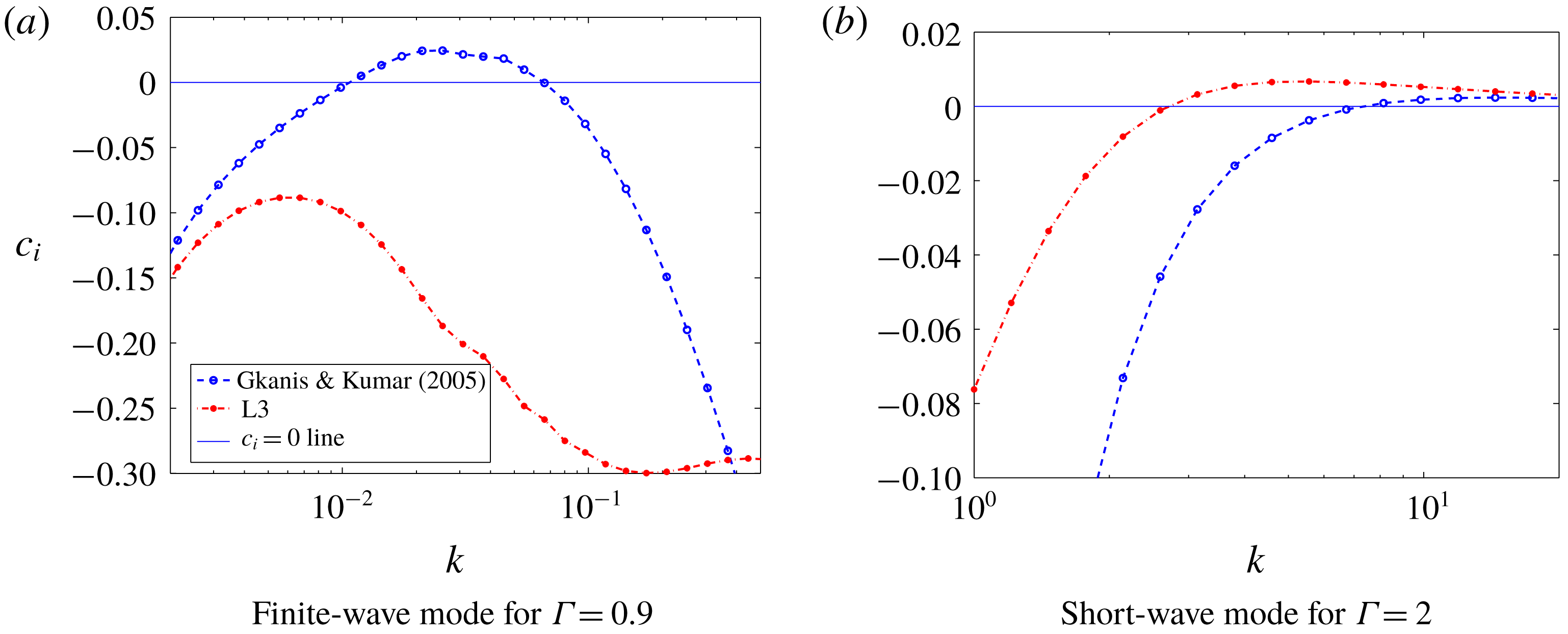
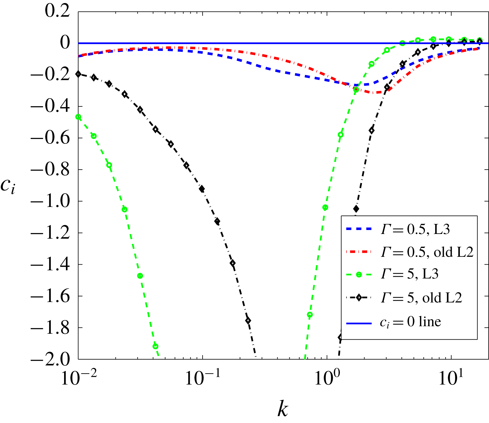
Gkanis & Kumar (Reference Gkanis and Kumar2005) studied the stability of the plane Poiseuille flow through a neo-Hookean channel and predicted the presence of a finite-wave instability. However, we find that the L3 formulation predicts the absence of a finite-wave instability in the creeping-flow limit. To compare both formulations, we plot the variation of
 $c_{i}$
with
 $k$
of the most unstable (or least stable) varicose mode in figure 4(a,b) for
 $Re=0$
. Here, we refer to the most unstable (or least stable) eigenvalue as the one which has the largest magnitude of positive
 $c_{i}$
(or smallest value of negative
 $c_{i}$
). For unstable flows, the most unstable eigenvalue will dominate the stability of the system, and will be relevant to experimental observations. Figure 4(a) clearly shows the absence of the finite-wave instability for the L3 formulation predicted by Gkanis & Kumar (Reference Gkanis and Kumar2005). Figure 4(b) shows the presence of the short-wave instability for both formulations but they are not in quantitative agreement. A similar analysis was carried out for the sinuous modes (not shown here for the sake of brevity) and the conclusions were similar to the ones shown here for varicose modes. The disagreement between the L3 formulation and Gkanis & Kumar (Reference Gkanis and Kumar2005) shown in figure 4(a,b) is due to the inconsistent interface conditions of the latter. The inconsistency stems from Taylor expansion of the solid base-state quantities in the flow-normal direction by Gkanis & Kumar (Reference Gkanis and Kumar2005) even when a Lagrangian framework was used for the solid. Thus, the finite-wave instability predicted by Gkanis & Kumar (Reference Gkanis and Kumar2005) for plane Poiseuille through a neo-Hookean channel was a physically spurious instability due to the use of inconsistent interface conditions.
Variation of
 $c_{i}$
with
 $k$
for the most unstable or least stable varicose mode for plane Poiseuille flow through a neo-Hookean channel predicted by Gkanis & Kumar (Reference Gkanis and Kumar2005) and the L3 formulation of the present study. Panels (a) and (b) respectively show comparisons of both formulations for the finite-wave and short-wave instabilities. The other parameters are
 $Re=0,H=15$
and
 $T=0$
. The figure shows the disappearance of the finite-wave instability upon using the consistent L3 formulation.

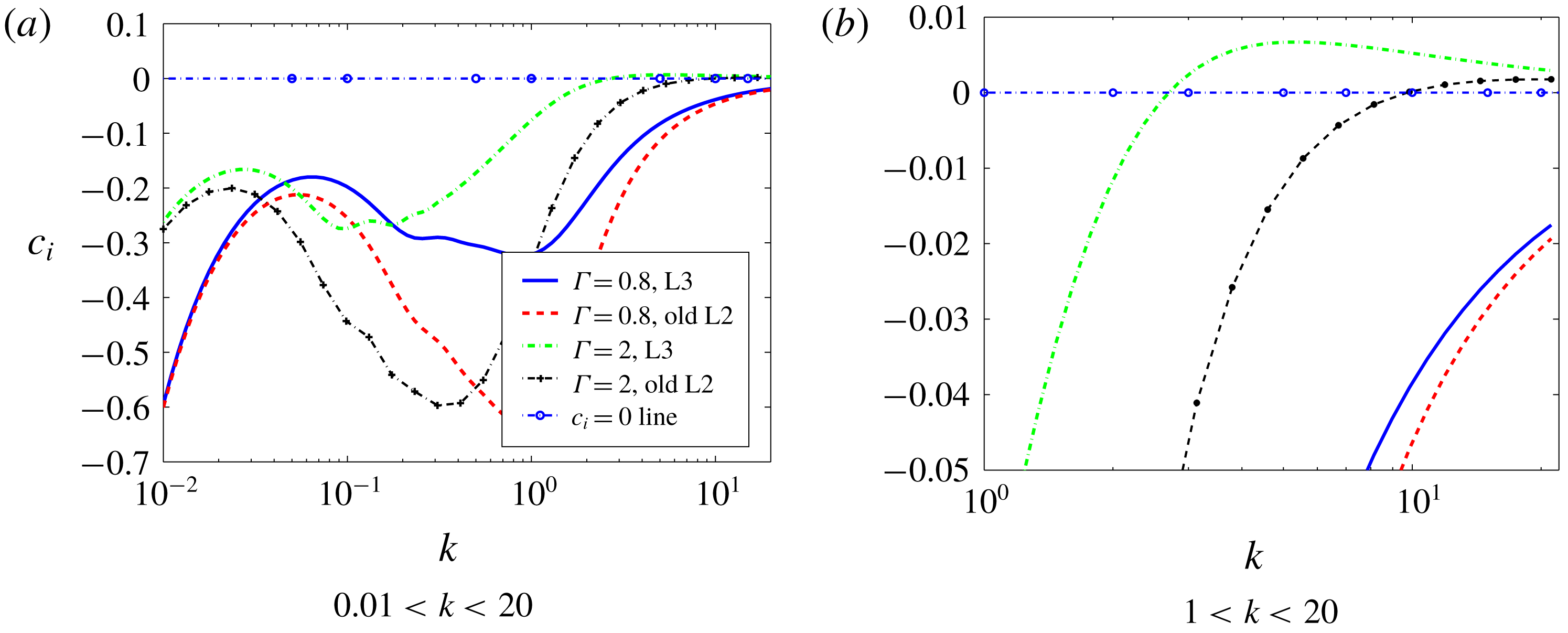
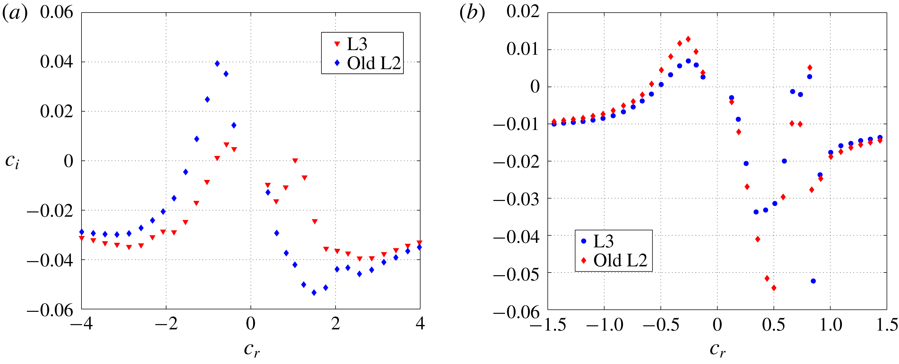
In the creeping-flow limit, the old L2 (i.e. Gaurav & Shankar (Reference Shankar2010)) formulation predicted only the short-wave instability for both varicose and sinuous modes. The eigenvalues obtained by using the old L2 and L3 formulations for varicose modes are compared in figure 5(a). Since the finite-wave instability was predicted to exist for
 $k<1$
and
 $\unicode[STIX]{x1D6E4}<1$
by Gkanis & Kumar (Reference Gkanis and Kumar2005), thus the curves for
 $\unicode[STIX]{x1D6E4}=0.8$
are plotted for both formulations and we observe the absence of the finite-wave instability for both formulations. We have verified (data not shown) that the results from the consistent Eulerian formulation also show the absence of the finite-wavenumber instability, and are in quantitative agreement with those obtained using the L3 formulation. To probe for short-wave instability, for varicose modes, dispersion curves (figure 5
a) are obtained for
 $\unicode[STIX]{x1D6E4}=2$
since
 $\unicode[STIX]{x1D6E4}_{c}>1$
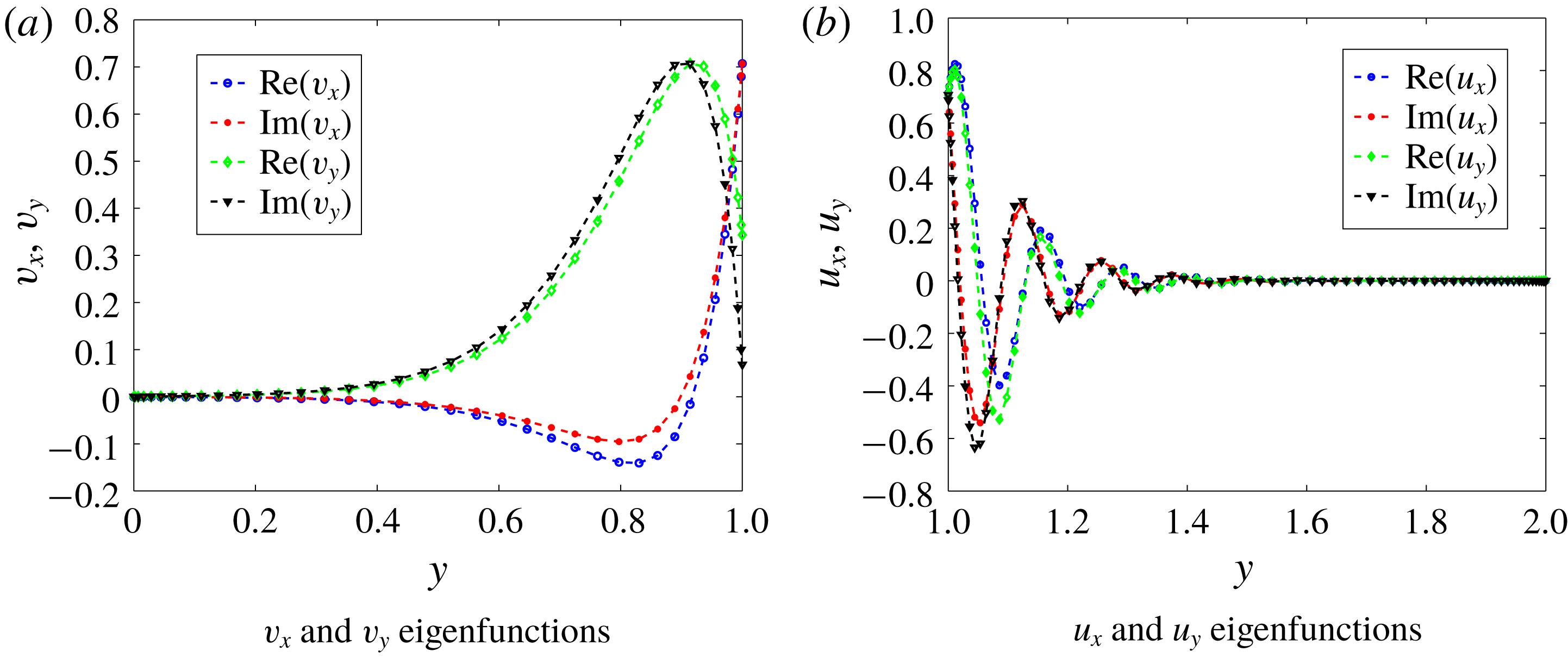
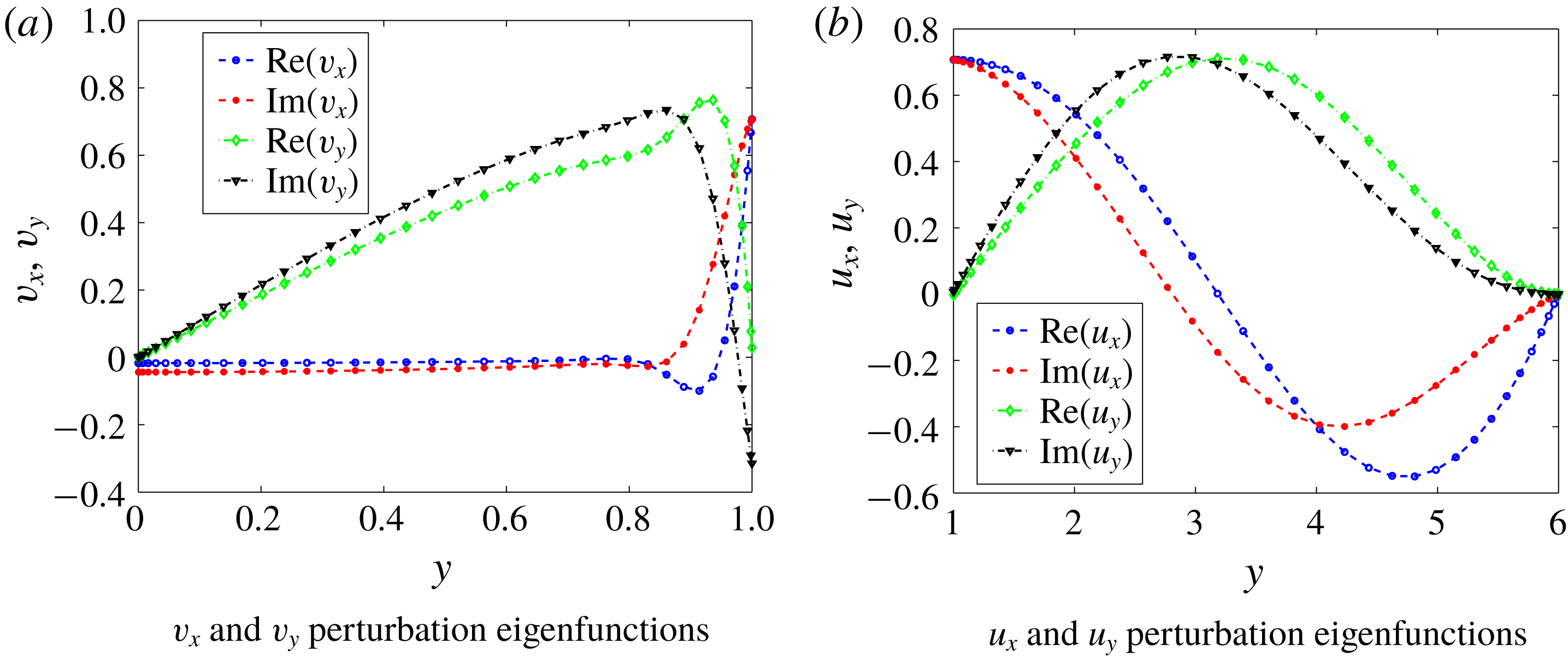
for the short-wave instability. Furthermore, from figure 5(b), we observe that the L3 formulation predicts instability for a different range of wavenumbers than the old L2 formulation. A similar conclusion for the sinuous mode was reached and for the sake of brevity here we show results only for the varicose modes. The similarity in results for sinuous and varicose modes for the short-wave instability can be explained by noting that the short-wave disturbances are confined (as shown in figure 6
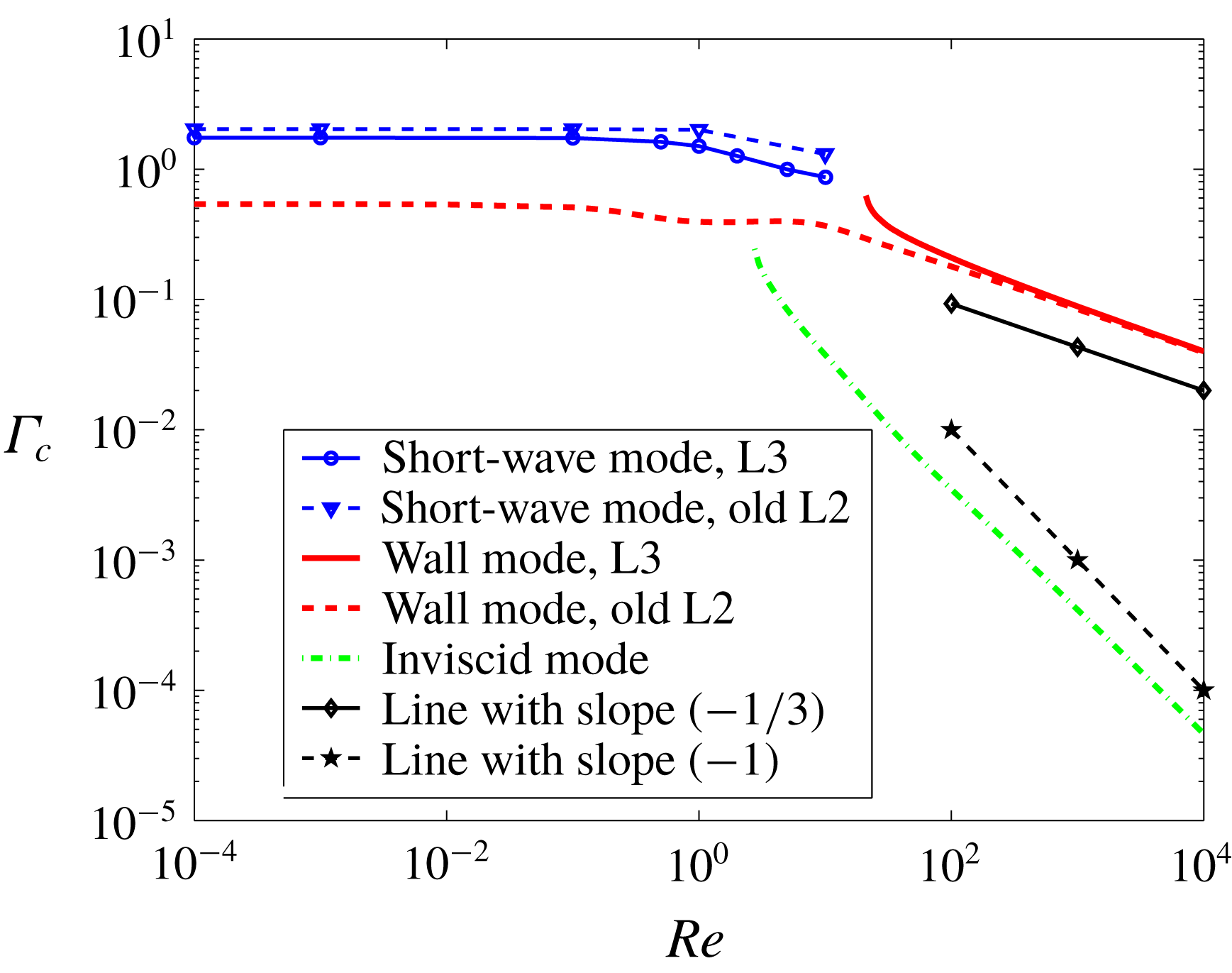
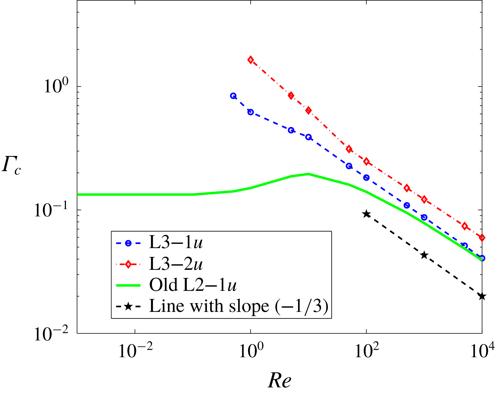
a) near the fluid–solid interface, and hence are not affected by the symmetry conditions imposed at the channel centreline. To compare the critical parameters predicted by two formulations, later in figure 11, the variation of
 $\unicode[STIX]{x1D6E4}_{c}$
with
 $Re$
for the short-wave instability is shown for both formulations.
Variation of
 $c_{i}$
with
 $k$
of the most unstable or least stable varicose mode for plane Poiseuille flow through a neo-Hookean channel at
 $Re=0,H=5$
and
 $T=0$
. Panel (a) shows curves for
 $0.01<k<20$
and the high-
 $k$
regime is magnified in panel (b). The figure shows the effect of using the consistent interface conditions on the most unstable (or least stable) mode.

The short-wave instability discussed above arises because of the jump in the first normal stress difference across the fluid–solid interface (Gkanis & Kumar Reference Gkanis and Kumar2003). To obtain more insight into the short-wave instability, we plot the eigenfunctions for the streamwise and normal velocities in figure 6(a) for the short-wave mode. The tangential and normal displacement eigenfunctions of the solid for the same eigenvalue are plotted in figure 6(b). The fluid and solid eigenfunctions show maximum variation near the fluid–solid interface (
 $y=1$
), showing the exchange of the energy which leads to the destabilisation of the short-wave mode. Further, both fluid velocities and solid displacements decay away from the fluid–solid interface, thus showing that the physics behind this instability is independent of the conditions at the channel centreline and the solid layer thickness
 $H$
.
Eigenfunctions of varicose modes in plane Poiseuille flow through a neo-Hookean channel at
 $Re=0,H=1,\unicode[STIX]{x1D6E4}=2,k=10$
and
 $T=0$
predicted by the L3 formulation. The eigenfunctions show the maximum variation near the fluid–solid interface.

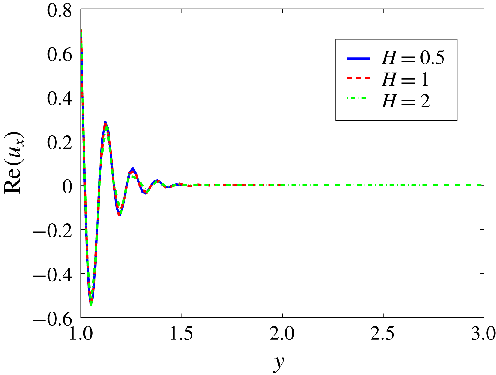
Interestingly, from figure 6(b), we observe that the disturbances in the solid are confined to
 $y<1.5$
. To verify whether the preceding conclusion about the confinement of the disturbances depends on the solid thickness
 $H$
, in figure 7, the displacement perturbation eigenfunctions are plotted for
 $H=0.5,1$
and
 $H=2$
. Figure 7 shows that, indeed, the disturbances are confined within
 $1<y<1.5$
, inside the solid, and the eigenfunctions for different values of
 $H$
are identical, thus showing that the instability is independent of
 $H$
. The thickness of the solid up to which perturbations penetrate, however, is a function of the wavenumber, because decrease in the wavenumber translates into an increase in the wavelength, thereby increasing the penetration of the disturbances inside the solid. To conclude, the penetration of disturbances in the solid layer is only a function of the wavenumber of the disturbances, and is independent of other parameters like
 $\unicode[STIX]{x1D6E4}$
,
 $H$
etc.
The
 $u_{x}$
perturbation eigenfunctions of varicose modes in plane Poiseuille flow through a neo-Hookean channel at
 $Re=0,\unicode[STIX]{x1D6E4}=2,k=10$
and
 $T=0$
predicted by the L3 formulation. Figure shows that the penetration of the disturbances in the solid is independent of
 $H$
and is restricted to
 $y<1.5$
.

3.1.2 Low-
 $Re$
(
$Re<10$
) limit


Gaurav & Shankar (Reference Shankar2010) predicted a class of unstable (varicose and sinuous) modes at low
 $Re$
(
 $Re\ll 1$
) which they ascribed to the destabilisation of the shear waves in the neo-Hookean solid. The instability predicted by Gaurav & Shankar (Reference Shankar2010) at low-
 $Re$
henceforth will be referred as the ‘low-
 $Re$
’ instability. These shear waves are present in an elastic solid for finite inertia (Achenbach Reference Achenbach1973) and are destabilised because of the shear applied by the fluid on the solid at the interface. However, we find that upon introducing consistent interface conditions, the low-
 $Re$
unstable modes predicted by Gaurav & Shankar (Reference Shankar2010) disappear and for
 $Re<1$
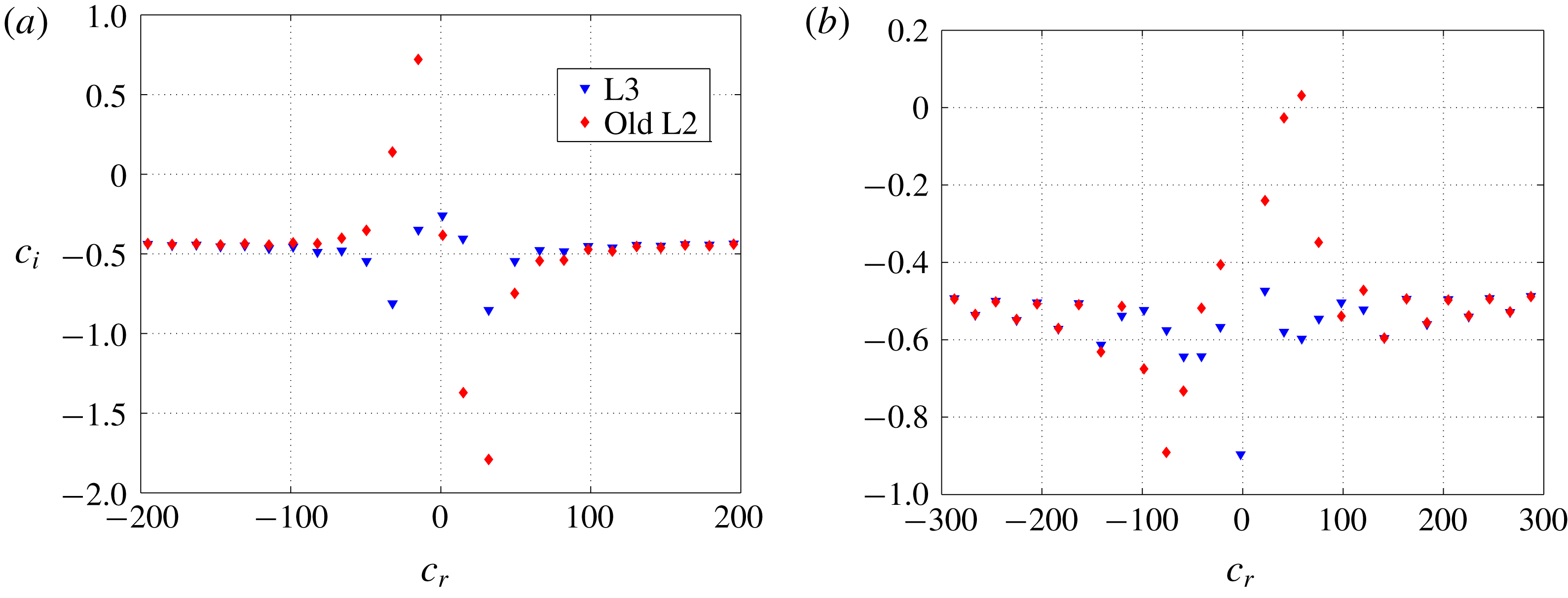
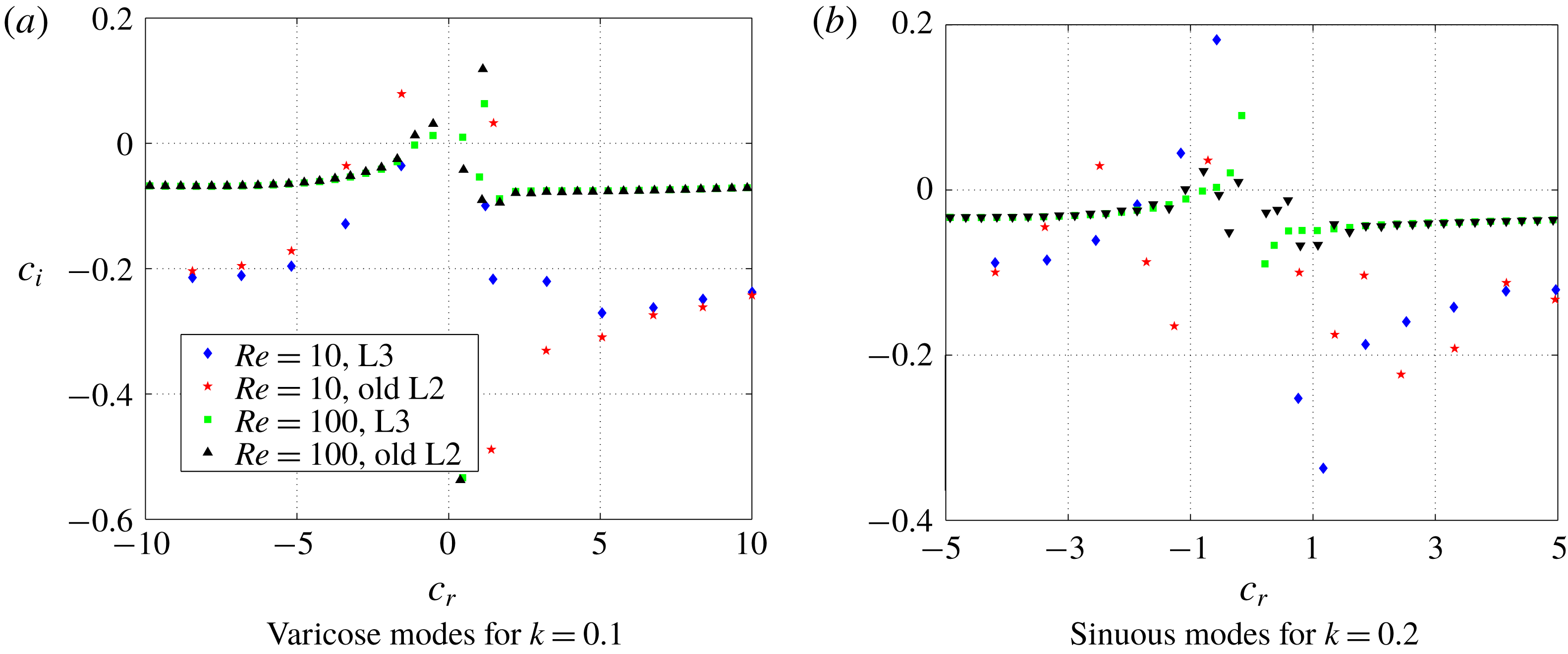
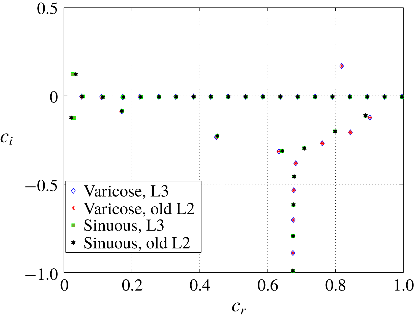
, it is the continuation of the short-wave instability that governs the stability behaviour of the system. To illustrate this, we compare the spectra obtained by using the old L2 and L3 formulations for varicose modes in figure 8(a) and observe that the L3 formulation does not predict the unstable modes in contrast to the old L2 formulation. The unstable upstream varicose modes (
 $c_{r}<0$
) predicted by the old L2 formulation and shown in figure 8(a) become unstable for
 $\unicode[STIX]{x1D6E4}<1$
. These modes, if continued to high
 $Re$
, show variation of
 $\unicode[STIX]{x1D6E4}_{c}$
proportional to
 $Re^{-1/3}$
(Gaurav & Shankar Reference Shankar2010) and are traditionally classified as the wall modes. However, these modes are absent when the consistent formulation is used. A similar comparison of spectra for sinuous modes is shown in figure 8(b). Gaurav & Shankar (Reference Shankar2010) predicted unstable downstream sinuous modes (
 $c_{r}>0$
) at low-
 $Re$
and these modes become inviscid modes at high
 $Re$
. However, as shown in figure 8(b), the L3 formulation does not predict any unstable downstream sinuous modes at low
 $Re$
owing to the consistent interface conditions.
Comparison of spectra obtained from the old L2 and L3 formulations for plane Poiseuille flow. Panel (a) compares varicose modes for
 $Re=0.1,H=5,\unicode[STIX]{x1D6E4}=1.5$
and
 $k=0.1$
while panel (b) compares sinuous modes for
 $Re=0.01,H=5,\unicode[STIX]{x1D6E4}=1.5$
and
 $k=0.25$
. Figure shows absence of the unstable upstream varicose and downstream sinuous modes in the spectra predicted by the L3 formulation in disagreement with the old L2 formulation (Gaurav & Shankar Reference Shankar2010).

The absence of unstable upstream varicose and downstream sinuous modes at low-
 $Re$
in the L3 formulation can be attributed to the additional interaction term (between the base-state pressure gradient and tangential displacement perturbation) introduced by the L3 formulation in the normal stress continuity (2.27). Since the low-
 $Re$
instability originated from the destabilisation of the shear waves in the solid due to the shear work done by the fluid at the fluid–solid interface, the interaction term between the base-state pressure gradient and tangential displacement perturbation stabilises these shear waves, possibly by extracting the energy provided by the fluid shear. Furthermore, we have verified that the results of the L3 formulation also agree with the consistent Eulerian formulation (Patne et al.
Reference Patne, Giribabu and Shankar2017) which does not have any ambiguity in the linearised interface conditions, thereby validating the analysis.
For
 $Re<1$
, the L3 formulation predicts short-wave instability as the critical mode and it persists for arbitrarily high wavenumber. The existence of unstable disturbances with arbitrarily high wavenumbers is termed the ‘Hadamard instability’ which is often associated with an inconsistent formulation or ill posedness of the problem (Joseph & Saut Reference Joseph and Saut1990). The Hadamard instability can be regularised by introducing physical effects, often small, such as surface tension, depending on the system under consideration (Joseph & Saut Reference Joseph and Saut1990). Thus the short-wave instability is also a Hadamard instability but Gkanis & Kumar (Reference Gkanis and Kumar2003) showed that it can be regularised by introducing finite value of the interface tension thereby putting an upper bound on the unstable wavenumber.
The physically realistic values of
 $T$
can be estimated as follows. For flow of water through a deformable channel, the dimensional interface tension is in the range
 $0.001{-}0.05~\text{N}~\text{m}^{-1}$
with the deformable wall of shear modulus 0.9–10 kPa and half-channel width of order
 $1~\unicode[STIX]{x03BC}\text{m}$
, the dimensionless surface tension,
 $T$
falls in the range
 $T=0.1{-}50$
since
 $T$
is the ratio of the dimensional surface tension and the product
 $GR$
. Here we take the lowest value of
 $T$
so as to show the effect of the consistent formulation on the critical parameters for the short-wave instability.
We later show in figure 11 the variation of
 $\unicode[STIX]{x1D6E4}_{c}$
with
 $Re$
at
 $T=0.1$
for the short-wave instability predicted by both formulations for varicose and sinuous modes. Figure 11 shows that the L3 formulation predicts lower value of
 $\unicode[STIX]{x1D6E4}_{c}$
than the old L2 formulation. For
 $Re<1$
, as shown in figure 11,
 $\unicode[STIX]{x1D6E4}_{c}$
for the short-wave instability varies to a negligible extent with
 $Re$
and for
 $Re>1$
,
 $\unicode[STIX]{x1D6E4}_{c}$
starts to deviate from the creeping-flow limit value without showing a concrete scaling similar to the wall or inviscid modes. For high
 $Re$
, numerically it is difficult to continue the short-wave mode and also
 $\unicode[STIX]{x1D6E4}_{c}$
for the short-wave mode is considerably higher than other modes of instability for
 $Re>10$
, implying that the short-wave mode will not be the critical mode and hence, the data for the short-wave mode are presented only for
 $Re<10$
.
3.1.3 Results at intermediate and high
$Re$

We next examine the effect of consistent interface conditions on the spectra at intermediate
 $Re$
(
 $10<Re<100$
) for both varicose and sinuous modes. As shown in figure 9(a), for
 $Re=10$
, the L3 formulation predicts varicose modes to be stable, while the old L2 formulation predicts two unstable modes of which one is upstream while other is downstream. Figures 8(a) and 9(a) show the disagreement between the old L2 and L3 formulations in predicting unstable upstream and downstream varicose modes at low and intermediate values of
 $Re$
. For sinuous modes, both formulations predict two unstable modes at
 $Re=10$
as shown in figure 9(b), but the quantitative difference between the eigenvalues predicted by the two formulations still persists. It must be noted that this seemingly minor quantitative difference has major consequences for predicting the critical mode of instability for the system, as discussed later.
Comparison of spectra obtained by using the old L2 and L3 formulations for plane Poiseuille flow. Panel (a) compares spectra of varicose modes, while panel (b) compares spectra of sinuous modes. The other parameters are
 $H=5,\unicode[STIX]{x1D6E4}=1.5$
and
 $T=0$
. Figure shows the effect of consistent interface conditions on the spectra at intermediate
 $Re$
and an improvement in agreement between two formulations as
 $Re$
is increased.

As
 $Re$
is increased, the spectra from both the formulations tend to agree as shown in figure 9(a,b) for
 $Re=100$
, implying that when inertial forces become dominant over elastic and viscous forces, interface conditions do not play a major role in determining the stability of the system. Indeed, as shown in figure 10 for
 $Re=1000$
, the disagreement between the two formulations is negligibly small and hence the predictions of Gaurav & Shankar (Reference Shankar2010) are valid in the limit of high
 $Re$
. To conclude, the disagreement between the old L2 and L3 formulations is present even at intermediate values of
 $Re$
and these could be significant from an experimental point of view as well. More careful experiments in this parameter regime will be needed to verify the predictions of this study.
Spectra of varicose and sinuous modes for parameters
 $Re=10^{4},H=5,k=0.1$
and
 $\unicode[STIX]{x1D6E4}=1.5$
for plane Poiseuille flow. The disagreement between the two formulations reduces as
 $Re$
increases.

We next study the effect of consistent interface conditions on the wall modes and inviscid modes predicted by Gaurav & Shankar (Reference Shankar2010) at high
 $Re$
. Figure 11 compares the critical conditions of the most unstable varicose wall mode for
 $H=5$
predicted by both formulations. In figure 11, the extension of the wall mode to low
 $Re$
for the old L2 formulation is the low-
 $Re$
instability, while for the L3 formulation the
 $\unicode[STIX]{x1D6E4}_{c}$
required for instability diverges to infinity at a finite
 $Re$
, showing the absence of the low-
 $Re$
instability. However, the results for both formulations asymptotically agree for high
 $Re$
and show the characteristic scaling
 $\unicode[STIX]{x1D6E4}_{c}\sim Re^{-1/3}$
. Also, the eigenvalues corresponding to wall modes predicted by both formulations are upstream modes.
Variation of
 $\unicode[STIX]{x1D6E4}_{c}$
with
 $Re$
of the varicose short-wave, most unstable wall and inviscid modes predicted by the old L2 and L3 formulations for plane Poiseuille flow. The parameters are
 $H=5$
and
 $T=0.1$
for short-wave mode while
 $T=0$
for wall and inviscid modes. Figure shows disagreement between the old L2 and L3 formulations in the case of varicose short-wave and most unstable wall modes.

For wall modes, viscous effects become important in the wall layer of thickness
 $Re^{-1/3}$
near the fluid–solid interface (Kumaran Reference Kumaran2000; Shankar & Kumaran Reference Shankar and Kumaran2002). The destabilising mechanism is the transfer of energy from the base-state flow to fluctuations due to the shear work done by the base-state flow at the interface (Kumaran Reference Kumaran2000). To understand the mechanism of destabilisation of the wall modes, we plot the eigenfunctions of the most unstable varicose wall mode at
 $Re=5000$
at the critical conditions (
 $k_{c}$
and
 $\unicode[STIX]{x1D6E4}_{c}$
) in figure 12(a) for the tangential and normal velocity perturbations of the fluid and in figure 12(b) for the tangential and normal displacement perturbation eigenfunctions of the solid. In figure 12(a), the fluid perturbations show maximum variation near the fluid–solid interface within a layer of thickness
 $Re^{-1/3}\approx 0.0585$
, i.e. in the interval
 $0.94<y\leqslant 1$
in agreement with the theoretical estimate. Similar eigenfunction plots were obtained for the old L2 formulation also (not shown here) and we found qualitative similarity between the eigenfunctions for the L3 and old L2 formulations showing that, at high
 $Re$
, the form of the eigenfunctions for the wall modes is independent of the formulation. Another important class of varicose modes of instability are the varicose inviscid modes. Figure 11 compares most unstable varicose inviscid mode for both formulations. As shown, the old L2 and L3 formulations agree and hence only a single curve is shown in figure 11. Similar to Gaurav & Shankar (Reference Shankar2010), we observe that the inviscid modes are downstream travelling modes.
Panel (a) shows the tangential and normal velocity perturbation eigenfunctions for the fluid while panel (b) shows the tangential and normal displacement perturbation eigenfunctions for the solid at
 $Re=5000,k=0.475,\unicode[STIX]{x1D6E4}=0.0505,H=5$
and
 $T=0$
for plane Poiseuille flow (varicose modes) using the L3 formulation. The maximum variation of the perturbations in the fluid near the fluid–solid interface explains the wall mode nature of the instability.

The above discussion for varicose modes shows that the two formulations disagree for varicose wall modes but agree for varicose inviscid modes. As pointed out earlier, the extension of the low-
 $Re$
instability predicted by Gaurav & Shankar (Reference Shankar2010) are varicose wall and sinuous inviscid modes, thus in the following discussion we analyse sinuous inviscid modes. Figure 13 compares variation of
 $\unicode[STIX]{x1D6E4}_{c}$
with
 $Re$
predicted by both formulations for the most unstable sinuous wall and inviscid modes where the L3 formulation predicts lower
 $\unicode[STIX]{x1D6E4}_{c}$
in comparison with the old L2 formulation for both types of sinuous modes. Despite quantitative differences, sinuous wall and inviscid modes predicted by both formulations are respectively upstream and downstream travelling modes. For sinuous inviscid modes, the high
 $Re$
part of the curve predicted by the old L2 formulation continues to
 $Re<0.1$
as low-
 $Re$
instability. However, the L3 formulation predicts divergence of the
 $\unicode[STIX]{x1D6E4}_{c}$
curve to infinite
 $\unicode[STIX]{x1D6E4}_{c}$
at low
 $Re$
as a consequence of the absence of low-
 $Re$
instability. Moreover for
 $Re<500$
, the old L2 formulation predicts lower
 $\unicode[STIX]{x1D6E4}_{c}$
than L3 formulation, but for
 $Re>500$
situation reverses, bearing important consequences for future experimental studies.
Variation of
 $\unicode[STIX]{x1D6E4}_{c}$
with
 $Re$
for the most unstable sinuous wall and inviscid modes for plane Poiseuille flow by using
 $H=5$
and
 $T=0$
. Figure shows disagreement between the old L2 and L3 formulations as the L3 formulation predicts lower
 $\unicode[STIX]{x1D6E4}_{c}$
than the old L2 formulation.

The inviscid mode of the instability arises where inertial stresses in the fluid are balanced by the elastic stresses in the deformable wall such that
 $\unicode[STIX]{x1D70C}V_{m}^{2}\sim G$
which upon using the definition of
 $\unicode[STIX]{x1D6E4}$
and
 $Re$
becomes,
 $\unicode[STIX]{x1D6E4}_{c}\sim Re^{-1}$
. The inviscid mode predicted in this study for plane and pipe Poiseuille flows is quite different from Rayleigh’s inflexion point instability for rigid surfaces for the following reason. An analogue of the inflexion point instability in a deformable channel and tube would exist in the purely inviscid limit (Yeo & Dowling Reference Yeo and Dowling1987; Shankar & Kumaran Reference Shankar and Kumaran1999, Reference Shankar and Kumaran2000), but the inviscid instabilities analysed in this paper exist in the limit
 $Re\gg 1$
but not in the complete absence of viscous effects. It must be noted that these modes are not the continuation of the Tollmien–Schlichting instability in rigid tubes and channels, since the critical Reynolds number is proportional to
 $(\unicode[STIX]{x1D70C}GR^{2}/\unicode[STIX]{x1D702}^{2})^{1/2}$
in the limit of large elasticity, whereas the critical Reynolds number of the Tollmien–Schlichting modes converges to a finite value in this limit (Kumaran Reference Kumaran2000). At high
 $Re$
, both formulations show a similar structure of the eigenfunctions as the dominance of the inertial terms masks the inconsistencies in the old L2 formulation. Thus only a quantitative difference is observed for the critical parameters. Figures 14(a) and 14(b) show the tangential and normal velocities and displacement eigenfunctions respectively in the fluid and solid. Since
 $k_{c}>1$
, the perturbations do not reach all the way to the deformable solid–rigid solid interface depending on the wavenumber, as shown in figure 14(b). This leads to an immediate conclusion that for
 $H>4$
the inviscid curves (shown for
 $H=5$
in figure 13) are independent of
 $H$
value. Thus, to introduce inviscid instability in the flow past deformable surfaces, there is a critical value of
 $H$
upon which any increment in
 $H$
,
 $\unicode[STIX]{x1D6E4}_{c}$
will not decrease. This hypothesis has been indeed verified (data not shown) for
 $Re=10^{4}$
for which we observed
 $\unicode[STIX]{x1D6E4}_{c}$
to vary to the fifth significant digit upon varying
 $H=5$
to
 $H=10$
.
Panel (a) shows the tangential and normal velocity perturbation eigenfunctions for the fluid while panel (b) shows the tangential and normal displacement perturbation eigenfunctions for the solid at
 $Re=7000,k_{c}=3.5,\unicode[STIX]{x1D6E4}_{c}=0.00014,H=5$
and
 $T=0$
for plane Poiseuille flow (sinuous modes) using the L3 formulation.

The preceding discussion on varicose and sinuous modes of instability provided a comparison for the wall and inviscid modes separately. However, from a practical point of view, it is important to determine the mode that dominates the stability of the system since this mode will be the one that is observed experimentally. Following Gaurav & Shankar (Reference Shankar2010), we plot the variation of critical
 $Re$
for a given fluid and deformable solid. This can be achieved by using the flow independent parameter
 $\unicode[STIX]{x1D6F4}=Re/\unicode[STIX]{x1D6E4}=\unicode[STIX]{x1D70C}GR^{2}/\unicode[STIX]{x1D702}^{2}$
. In the
 $Re{-}\unicode[STIX]{x1D6F4}$
plane, the short-wave, inviscid and wall modes respectively show characteristic scaling of
 $Re\sim \unicode[STIX]{x1D6F4}$
,
 $Re\sim \unicode[STIX]{x1D6F4}^{1/2}$
and
 $Re\sim \unicode[STIX]{x1D6F4}^{3/4}$
(Gaurav & Shankar Reference Shankar2010). Figures 15(a) and 15(b) respectively show the variation of
 $Re$
with
 $\unicode[STIX]{x1D6F4}$
obtained from both the L3 and old L2 formulations. The old L2 formulation (figure 15
b) predicts the most unstable sinuous inviscid mode as the critical mode for region
 $\unicode[STIX]{x1D6F4}<10^{3}$
and for
 $\unicode[STIX]{x1D6F4}>10^{3}$
, the most unstable varicose inviscid mode is the critical mode. In other words, according to the predictions of the old L2 formulation, inviscid modes determine the stability of the system.
Variation of critical
 $Re$
with
 $\unicode[STIX]{x1D6F4}$
for plane Poiseuille flow for
 $H=5$
. Panels (a) and (b) respectively show predictions from the L3 and old L2 formulations for a given fluid and solid. R1, R2 and R3 are respectively reference lines with slopes 1,
 $3/4$
and
 $1/2$
. WM and IM are respectively abbreviations for wall and inviscid modes. For
 $\unicode[STIX]{x1D6F4}<1$
, the old L2 formulation predicts a sinuous inviscid mode while the L3 formulation predicts a short-wave mode as the most unstable mode.

However, the same is not true for the L3 formulation (figure 15
a). To compare, the old L2 formulation predicts that the short-wave mode does not play any role in determining the stability of the system unlike in the case of the L3 formulation where the short-wave mode determines the stability behaviour of the system for
 $\unicode[STIX]{x1D6F4}<1$
. For
 $1<\unicode[STIX]{x1D6F4}<10$
, according to the L3 formulation, the most unstable mode is the sinuous wall mode unlike in the case of old L2 formulation for which the wall mode does not determine the stability of the system for any value of
 $\unicode[STIX]{x1D6F4}$
. For
 $\unicode[STIX]{x1D6F4}>10$
, the L3 formulation predicts the most unstable mode varicose inviscid mode as the critical mode, similar to the old L2 formulation.
It must be noted that the experiments for flow past deformable surfaces are able to observe the instability due to wall modes alone (Verma & Kumaran Reference Verma and Kumaran2012, Reference Verma and Kumaran2013). Hence, it is important to compare wall modes predicted by both formulations. Comparison of figures 15(a) and 15(b) shows that the L2 formulation predicts the varicose wall mode to be more unstable than the sinuous wall mode, opposite to the L3 formulation. Hence experiments carried out for plane Poiseuille flow through a neo-Hookean channel can potentially discriminate between the two formulations.
3.2 Hagen–Poiseuille flow through a neo-Hookean tube
In this section we compare results obtained by using the present L3 formulation and results of Gaurav & Shankar (Reference Shankar2009). As noted in § 2.3, the linearised perturbation equations in the L3 formulation of Hagen–Poiseuille flow through a neo-Hookean tube can be obtained from the Hagen–Poiseuille flow through a Mooney–Rivlin tube by substituting
 $\unicode[STIX]{x1D6FD}=0$
and
 $C_{1}=G/2$
.
3.2.1 Creeping-flow limit
Figure 16 compares variation of
 $c_{i}$
with
 $k$
for
 $Re=0$
and
 $H=5$
as predicted by the old L2 and L3 formulations. Similar to plane Poiseuille flow through a neo-Hookean channel the L3 formulation shows an absence of the finite-wave instability and exhibits only the short-wave instability, in agreement with the old L2 formulation and in disagreement with Kumaran (Reference Kumaran1995a
). However,
 $\unicode[STIX]{x1D6E4}_{c}$
is lower for the L3 formulation in comparison with the old L2 formulation. The disagreement between the present study and Kumaran (Reference Kumaran1995a
) regarding the finite-wave instability is because of the inapplicability of the linear viscoelastic model to finite base-state deformations.
The variation of
 $c_{i}$
with
 $k$
for Hagen–Poiseuille flow through a neo-Hookean tube predicted by the old L2 and L3 formulations for
 $Re=0,T=0$
and
 $H=5$
. The figure shows the absence of the finite-wave instability for both the old L2 and L3 formulations.

3.2.2 Low-
$Re$
(
$Re<10$
) results


Gaurav & Shankar (Reference Shankar2009) predicted low-
 $Re$
instability which arises because of the destabilisation of the shear waves similar to the case of plane Poiseuille flow. However, we find that the low-
 $Re$
instability predicted by Gaurav & Shankar (Reference Shankar2009) is absent after using the L3 formulation. Figure 17 shows the disagreement between the old L2 and L3 formulations as the latter does not predict low-
 $Re$
instability. The absence of any other instability in the predictions of the L3 formulation for low
 $Re$
makes the short-wave mode of instability the critical mode. However, the short-wave instability shows negligible variation with the Reynolds number for low
 $Re$
as shown in figure 21. Consequently, the low
 $Re$
regime shows behaviour similar to the creeping-flow limit.
Eigenvalues in
 $c_{r}$
–
 $c_{i}$
plane at
 $Re=0.001,H=9,\unicode[STIX]{x1D6E4}=0.3$
and
 $k=0.01$
for Hagen–Poiseuille flow. Figure shows the absence of the low-
 $Re$
instability in the spectra of the L3 formulation, in disagreement with the old L2 formulation.

3.2.3 Intermediate and high
$Re$
results

The low-
 $Re$
instability of Gaurav & Shankar (Reference Shankar2009) gives rise to wall modes at high
 $Re$
and hence the absence of the low-
 $Re$
instability in the L3 formulation makes it necessary to study the effect of consistent interface conditions at high
 $Re$
. For
 $Re=10$
, figure 18(a) shows that both formulations predict unstable upstream modes but there is quantitative disagreement between the two spectra. Further, in figure 18(a), the old L2 formulation does not show any downstream unstable eigenvalue but the L3 formulation does. As predicted by Gaurav & Shankar (Reference Shankar2009) using the old L2 formulation, the upstream modes are the wall modes and these modes are also extensions of the low-
 $Re$
unstable modes. However, the L3 formulation predicts an additional downstream mode which shows scaling corresponding to an inviscid mode at high
 $Re$
, as discussed later. Figure 18(b) extends the comparison between two formulations to
 $Re=100$
which shows some improvement in agreement between the two formulations with increase in
 $Re$
. Taking into consideration figure 18(a,b), we reach the conclusion that there is substantial disagreement between both formulations even at
 $Re=100$
and disagreement decreases as
 $Re$
increases.
Comparison of spectra obtained by using both formulations for Hagen–Poiseuille flow. Panels (a) and (b) respectively compare spectra for
 $Re=10$
and
 $Re=100$
predicted by the old L2 and L3 formulations for
 $H=5,\unicode[STIX]{x1D6E4}=1$
and
 $k=0.75$
. The old L2 and L3 formulations disagree in predicting unstable eigenvalues and the disagreement decreases as inertial effects become dominant.

We next track the unstable eigenvalues to high
 $Re$
, in order to determine whether they are wall or inviscid modes. Figure 19 compares the wall modes predicted by both formulations, where ‘u’ stands for upstream and the number associated with it denotes the number of the mode in the sequence such that the modes are arranged in ascending order of
 $\unicode[STIX]{x1D6E4}_{c}$
. For example, ‘L3-1u’ stands for the most unstable upstream mode predicted by the L3 formulation. As shown in figure 19, unlike in the case of old L2 formulation, the continuation of wall modes to low
 $Re$
results in
 $\unicode[STIX]{x1D6E4}_{c}$
diverging at a finite
 $Re$
, thus indicating that these modes do not continue all the way to
 $Re\ll 1$
. The cause of this divergence is the absence of the low-
 $Re$
instability, unlike the old L2 formulation for which upstream travelling wall modes smoothly continue in the low
 $Re$
region because of the low-
 $Re$
instability. Furthermore, we observe that both the formulations predict all upstream modes as wall modes, of which the two most unstable modes predicted by the L3 formulation and most unstable mode predicted by the old L2 formulation are shown in figure 19. Furthermore, we observe the eigenfunctions and destabilisation mechanism for the wall modes predicted here are similar to those of plane Poiseuille flow through a neo-Hookean channel described in § 3.1.
Variation of
 $\unicode[STIX]{x1D6E4}_{c}$
with
 $Re$
for wall (upstream) modes predicted by both formulations for Hagen–Poiseuille flow through a neo-Hookean tube. Figure shows differences between the wall modes predicted by two formulations at
 $H=5$
and
 $T=0$
.

Figure 18(a) shows the downstream modes predicted by the L3 formulation have lower
 $\unicode[STIX]{x1D6E4}_{c}$
than the ones predicted by the old L2 formulation. For
 $Re<10^{4}$
, the old L2 formulation predicts
 $\unicode[STIX]{x1D6E4}_{c}$
values for the inviscid modes considerably higher than the wall modes and thus Gaurav & Shankar (Reference Shankar2009) concentrated on the wall modes alone in their analysis. Hence before proceeding with the analysis of inviscid modes predicted by the L3 formulation, we compare the two classes of downstream modes (i.e. inviscid and wall modes) predicted by both formulations. Figure 20 for
 $H=9$
and
 $k=1$
compares the most unstable downstream inviscid and wall modes obtained by using both formulations. As shown in figure 20, the L3 formulation predicts lower
 $\unicode[STIX]{x1D6E4}$
for the most unstable downstream inviscid and wall modes than the L2 formulation. This is not just a quantitative difference because the L3 formulation predicts
 $\unicode[STIX]{x1D6E4}_{c}$
to be lower for inviscid modes than the wall modes but the opposite is true for the old L2 formulation. Figure 20 also indicates that, to understand the stability behaviour of the system, we need to analyse the inviscid modes as well.
Variation of
 $\unicode[STIX]{x1D6E4}$
required for instability at
 $k=1,H=9$
and
 $T=0$
with
 $Re$
for downstream travelling predicted by both formulations for Hagen–Poiseuille flow through a neo-Hookean tube. Figure illustrates the destabilising role of the L3 formulation on downstream modes.

Figure 21 shows the variation of the value of
 $\unicode[STIX]{x1D6E4}_{c}$
for the two most unstable inviscid modes referred to as ‘1d’ and ‘2d’, respectively, meaning the first and second downstream modes. Additionally, we observe that all inviscid modes are downstream travelling modes with
 $c_{r}/\unicode[STIX]{x1D6E4}_{c}\sim 1$
in the present non-dimensionalisation scheme. Comparison of figures 19 and 21 shows the inviscid mode as the critical mode of instability for the L3 formulation.
Variation of
 $\unicode[STIX]{x1D6E4}_{c}$
with
 $Re$
for two most unstable inviscid modes predicted by the L3 formulation and short-wave mode predicted by both formulations for
 $H=5$
and
 $T=0$
for Hagen–Poiseuille flow through a neo-Hookean tube. Figure illustrates decrease in
 $\unicode[STIX]{x1D6E4}_{c}$
for the inviscid and short-wave modes using the L3 formulation.

To summarise the results for Hagen–Poiseuille flow through a neo-Hookean tube, we define the flow independent parameter
 $\unicode[STIX]{x1D6F4}=Re/\unicode[STIX]{x1D6E4}=\unicode[STIX]{x1D70C}GR_{t}^{2}/\unicode[STIX]{x1D702}^{2}$
and plot the variation of critical
 $Re$
with
 $\unicode[STIX]{x1D6F4}$
. Figures 22(a) and 22(b) respectively plot the variation of the critical
 $Re$
with
 $\unicode[STIX]{x1D6F4}$
for the old L2 and L3 formulations. The old L2 formulation predicts the most unstable wall mode as the critical mode for non-zero values of
 $Re$
. However, the L3 formulation predicts the short-wave mode to be the critical mode for
 $\unicode[STIX]{x1D6F4}<0.1$
and the most unstable inviscid mode as the critical mode for
 $\unicode[STIX]{x1D6F4}>1$
. It must be noted that the experiments of Verma & Kumaran (Reference Verma and Kumaran2012) on Hagen–Poiseuille flow through a neo-Hookean tube could not observe inviscid mode instability, but the wall modes were observed and, as shown in figure 19, for wall modes the disagreement between the
 $\unicode[STIX]{x1D6E4}_{c}$
predicted by both formulations for the range of
 $Re$
covered in the experiments by Verma & Kumaran (Reference Verma and Kumaran2012) is not large enough to be detected within experimental error. Hence to discern the effect of consistent formulations, experiments in the regime
 $Re<100$
are necessary.
Comparison of critical
 $Re$
predicted by both formulations for Hagen–Poiseuille flow and
 $H=5$
. Critical
 $Re$
for the old L2 formulation is determined by the most unstable wall mode while for the L3 formulation by the most unstable inviscid mode. R1, R2 and R3 are respectively reference lines with slopes
 $1$
,
 $3/4$
and
 $1/2$
.

3.3 Three-dimensional stability of the planar flows past a neo-Hookean solid
Patne et al. (Reference Patne, Giribabu and Shankar2017) proved the equivalence between the Eulerian and Eulerian (CK) formulations for planar flows subjected to two-dimensional disturbances and ascribed this equivalence to the simple kinematics of deformation in that configuration. Further, Patne et al. (Reference Patne, Giribabu and Shankar2017) speculated the possibility of the disagreement between the two formulations if planar flow is subjected to three-dimensional perturbations. Hence, in this section, we consider the stability analysis of the planar flow past a neo-Hookean solid subjected to three-dimensional disturbances by using the L3, Eulerian and Eulerian (CK) formulations. The base-state and linearised perturbation equations in the L3 formulation for planar flows can be obtained from the equations presented in appendix A by substituting
 $\unicode[STIX]{x1D6FD}=0$
and
 $C_{1}=G/2$
. Hence,
 $\unicode[STIX]{x1D6FE}$
, the dimensionless maximum base-state speed defined, can be redefined as
 $\unicode[STIX]{x1D6FE}=(\unicode[STIX]{x1D702}V_{m})/(GR)=\unicode[STIX]{x1D6E4}$
for plane Poiseuille flow and
 $\unicode[STIX]{x1D6FE}=(\unicode[STIX]{x1D702}V_{c})/(2GR)=\unicode[STIX]{x1D6E4}$
for plane Couette flow. The linearised perturbations equations in the Eulerian and Eulerian(CK) formulations for planar flows are derived in appendix B.
3.3.1 Plane Poiseuille flow
Table 5 shows the most unstable (or least stable) mode obtained by using all three formulations. Here we use growth rate,
 $s$
instead of the complex wave speed (
 $c$
) in order to analyse the stability of purely spanwise disturbances (for which
 $k=0$
), hence for the system to become temporally unstable the real part of the growth rate must be positive (
 $s_{r}>0$
). It must be noted that for
 $k\neq 0$
, the growth rate and complex wave speed are related by
 $s=-\text{i}kc$
. The first two rows in table 5 show agreement among all three formulations for which
 $m=0$
, i.e. two-dimensional perturbations. However, as
 $m$
takes non-zero values, the L3 and Eulerian (CK) formulation start to differ. As
 $m$
is increased, the Eulerian (CK) formulation shows a new instability while the L3 and Eulerian formulations show stabilisation. For
 $k=0$
, the Eulerian (CK) instability becomes most unstable showing a purely spanwise nature.
Eigenvalues predicted by the Eulerian, Eulerian (CK) and L3 formulations for viscous plane Poiseuille flow past a neo-Hookean solid at
 $Re=0$
. Data show agreement between the Eulerian and L3 formulations and disagreement between the Eulerian (CK) and L3 formulations in the creeping-flow limit.

Figure 23 shows that, as
 $k$
is increased to non-zero values, the spanwise instability in the Eulerian (CK) formulation is stabilised. Thus, the Eulerian and L3 formulations agree while L3 and Eulerian (CK) formulations disagree owing to the spanwise instability predicted by the latter. Figure 24 shows the disagreement between the Eulerian (CK) and L3 formulations for arbitrary
 $Re$
in
 $s_{i}$
–
 $s_{r}$
space and again the disagreement is because of the spanwise instability predicted by the Eulerian (CK) formulation. This also suggests that the Eulerian (CK) formulation predicts the spanwise mode as the critical mode for low
 $Re$
, unlike the L3 formulation.
The variation of
 $s_{r}$
with
 $m$
for plane Poiseuille flow past a neo-Hookean solid with
 $Re=0,\unicode[STIX]{x1D6E4}=1$
and
 $H=5$
predicted by the Eulerian (CK) and Eulerian formulations. Figure confirms disagreement between the Eulerian and Eulerian (CK) formulations.

Spectra in the
 $s_{i}{-}s_{r}$
plane for
 $Re=1,\unicode[STIX]{x1D6E4}=1,k=0.1,m=0.5$
and
 $H=5$
predicted by all three formulations for plane Poiseuille flow past a neo-Hookean solid. Figure shows agreement between the Eulerian and L3 formulations and disagreement between the L3 and Eulerian (CK) formulations for non-zero values of
 $Re$
.

3.3.2 Plane Couette flow
Similar to plane Poiseuille flow, the Eulerian (CK) formulation for plane Couette flow past a neo-Hookean solid predicts spanwise instability, as shown in table 6. However, the experimental findings of Kumaran & Muralikrishnan (Reference Kumaran and Muralikrishnan2000) and Neelmegam, Giribabu & Shankar (Reference Neelmegam, Giribabu and Shankar2014) agree with the L3 formulation predictions and they found only two-dimensional finite-wave instability in the
 $Re\ll 1$
limit for
 $H>1$
. The spanwise instability predicted by the Eulerian (CK) formulation was not experimentally observed, as discussed below.
The purely spanwise instability results in unstable disturbances with arbitrarily small wavelengths, as shown in figure 25. This shows the Hadamard nature of the purely spanwise instability. As discussed in § 3.1, the Hadamard nature of the short-wave instability can be regularised by introducing a finite value of the interfacial tension. A similar attempt to regularise the spanwise instability predicted by the Eulerian (CK) formulation, however, shows that the Hadamard nature of the instability does not disappear, as shown in figure 25. The inability to regularise the Hadamard nature of the spanwise instability even after introducing interfacial tension indicates that the inconsistency of the Eulerian (CK) formulation cannot be regularised. This lack of regularisation stems from the inconsistent constitutive model employed by the Eulerian (CK) formulation. More importantly, for the values of
 $\unicode[STIX]{x1D6E4}$
for which the purely spanwise instability is predicted by the Eulerian (CK) model, there is no evidence of an instability in the experimental observations of Kumaran & Muralikrishnan (Reference Kumaran and Muralikrishnan2000), Eggert & Kumar (Reference Eggert and Kumar2004).
The variation of
 $s_{r}$
with
 $m$
for plane Couette flow past a deformable solid with
 $Re=0,\unicode[STIX]{x1D6E4}=2,k=0$
and
 $H=0.1$
predicted by the Eulerian (CK) formulation. Figure shows the presence of the Hadamard instability and inability to regularise by using interfacial tension.

Eigenvalues predicted by the Eulerian, Eulerian (CK) and L3 formulations for plane Couette flow past a neo-Hookean solid at
 $Re=0$
. Data show disagreement between the Eulerian (CK) and L3 formulations.

The above discussion illustrates the spurious nature of the spanwise instability predicted by the Eulerian (CK) formulation. The presence of this instability for an arbitrary planar shear flow could be explained as follows. For a general planar shear flow the base-state Cauchy stress tensor in the Eulerian (CK) formulation is
 $$\begin{eqnarray}\displaystyle \bar{\unicode[STIX]{x1D748}}=\left[\begin{array}{@{}ccc@{}}\displaystyle \frac{1}{\unicode[STIX]{x1D6E4}}-\bar{p}_{g} & \displaystyle \frac{1}{\unicode[STIX]{x1D6E4}}\frac{\text{d}\bar{u}_{x}}{\text{d}\bar{y}} & 0\\ \displaystyle \frac{1}{\unicode[STIX]{x1D6E4}}\frac{\text{d}\bar{u}_{x}}{\text{d}\bar{y}} & \displaystyle \frac{1}{\unicode[STIX]{x1D6E4}}-\bar{p}_{g}-\frac{1}{\unicode[STIX]{x1D6E4}}\left(\frac{\text{d}\bar{u}_{x}}{\text{d}\bar{y}}\right)^{2} & 0\\ \displaystyle 0 & 0 & \displaystyle \frac{1}{\unicode[STIX]{x1D6E4}}-\bar{p}_{g}\end{array}\right]. & & \displaystyle\end{eqnarray}$$
Thus, the first and second normal stress differences for the Eulerian (CK) formulation are respectively,
 $\unicode[STIX]{x1D70E}_{xx}-\unicode[STIX]{x1D70E}_{yy}=(1/\unicode[STIX]{x1D6E4})(\text{d}\bar{u}_{x}/\text{d}\bar{y})^{2}$
and
 $\unicode[STIX]{x1D70E}_{yy}-\unicode[STIX]{x1D70E}_{zz}=-(1/\unicode[STIX]{x1D6E4})(\text{d}\bar{u}_{x}/\text{d}\bar{y})^{2}$
. Similarly for the consistent Eulerian formulation,
 $$\begin{eqnarray}\displaystyle \bar{\unicode[STIX]{x1D748}}=\left[\begin{array}{@{}ccc@{}}\displaystyle \frac{1}{\unicode[STIX]{x1D6E4}}-\bar{p}_{g}+\frac{1}{\unicode[STIX]{x1D6E4}}\left(\frac{\text{d}\bar{u}_{x}}{\text{d}\bar{y}}\right)^{2} & \displaystyle \frac{1}{\unicode[STIX]{x1D6E4}}\frac{\text{d}\bar{u}_{x}}{\text{d}\bar{y}} & 0\\ \displaystyle \frac{1}{\unicode[STIX]{x1D6E4}}\frac{\text{d}\bar{u}_{x}}{\text{d}\bar{y}} & \displaystyle \frac{1}{\unicode[STIX]{x1D6E4}}-\bar{p}_{g} & 0\\ 0 & 0 & \displaystyle \frac{1}{\unicode[STIX]{x1D6E4}}-\bar{p}_{g}\end{array}\right]. & & \displaystyle\end{eqnarray}$$
The first and second normal stress differences respectively are,
 $\unicode[STIX]{x1D70E}_{xx}-\unicode[STIX]{x1D70E}_{yy}=(1/\unicode[STIX]{x1D6E4})(\text{d}\bar{u}_{x}/\text{d}\bar{y})^{2}$
and
 $\unicode[STIX]{x1D70E}_{yy}-\unicode[STIX]{x1D70E}_{zz}=0$
. The non-zero second normal stress difference predicted by the Eulerian (CK) formulation creates additional coupling terms in the linearised perturbation equations which possibly create a bridge between the base state and perturbations, thereby giving rise to the predicted instability. To summarise, the Eulerian (CK) formulation disagrees with the Eulerian or L3 formulations even for planar flows subjected to three-dimensional disturbances owing to the non-zero second normal stress difference. Also, the predictions of the Eulerian (CK) formulation disagree with the experiments, thereby proving its inapplicability to study the stability of fluid flows past deformable surfaces.
3.4 Stability of flows past a Mooney–Rivlin solid
Patne et al. (Reference Patne, Giribabu and Shankar2017) found that for the Hagen–Poiseuille flow through a neo-Hookean tube the Eulerian (CK) formulation predicts a finite-wave instability in the creeping-flow limit, in disagreement with the L3 formulation. The disagreement arises because of the inconsistent neo-Hookean model in the Eulerian (CK) formulation as it is in fact a special case of the Mooney–Rivlin model (refer to table 2). From table 2, the linear combination of the constitutive equations for the Eulerian (B 3) and Eulerian (CK) (B 19) formulations forms a constitutive equation similar to Mooney–Rivlin model with
 $C_{1}=G/2$
and
 $C_{2}=G/2$
. Since the Eulerian (CK) formulation predicted finite-wave instability for Hagen–Poiseuille flow through a deformable tube, then the Mooney–Rivlin model may predict finite-wave instability owing to the Eulerian (CK) part. In § 3.3, the Eulerian (CK) formulation predicted a purely spanwise instability for planar flows past a neo-Hookean solid subjected to three-dimensional disturbances and the presence of the spanwise instability was ascribed to the non-zero second normal stress difference. This points to the possibility of a destabilising role of the non-zero second normal stress difference. The simplest model that has non-zero second normal stress difference is the Mooney–Rivlin model. Consequently, in this section we explore whether it is possible to find the existence of the finite-wave instability for flow through a Mooney–Rivlin tube and purely spanwise instability for planar flows past a Mooney–Rivlin solid within practically admissible values of
 $C_{1}$
and
 $C_{2}$
, thereby understanding the effect of the change of solid model on the stability of the system.
3.4.1 Planar flows past a Mooney–Rivlin solid
The linearised perturbation equations for planar flows past a Mooney–Rivlin solid subjected to three-dimensional perturbations are given in appendix A. In order to interpret the results in this section we use the substitution
 $s=-\text{i}kc$
in the equations of appendix A as
 $k\neq 0$
in this section. The dimensionless base-state speed defined for a Mooney–Rivlin solid,
 $\unicode[STIX]{x1D6FE}$
, which was used while deriving the governing equations, is not the correct parameter to compare with
 $\unicode[STIX]{x1D6E4}=\unicode[STIX]{x1D702}V_{m}/(GR)$
, the dimensionless base-state speed for a neo-Hookean solid, because for a Mooney–Rivlin solid the shear modulus is
 $G\approx 2(C_{1}+C_{2})$
(Holzapfel Reference Holzapfel2000). Hence, we redefine the dimensionless speed for the Mooney–Rivlin solid as
 $\unicode[STIX]{x1D6E4}_{m}=\unicode[STIX]{x1D702}V_{m}/(2(C_{1}+C_{2})R)=\unicode[STIX]{x1D6FE}/(1+\unicode[STIX]{x1D6FD})$
for plane Poiseuille flow and
 $\unicode[STIX]{x1D6E4}_{m}=\unicode[STIX]{x1D702}V_{c}/(4(C_{1}+C_{2})R)=\unicode[STIX]{x1D6FE}/(1+\unicode[STIX]{x1D6FD})$
for plane Couette flow where
 $\unicode[STIX]{x1D6FD}=C_{2}/C_{1}$
. It must be noted that,
 $\unicode[STIX]{x1D6FD}$
is restricted to the closed interval
 $[0,1]$
for a realistic hyperelastic solid. For example, silicone rubber has a value
 $\unicode[STIX]{x1D6FD}\approx 0.95$
(Macosko Reference Macosko1994) and for vulcanised natural rubber
 $\unicode[STIX]{x1D6FD}=0.1429$
(Anand Reference Anand1986).
Figure 26(a) shows the stabilising effect of the non-zero second normal stress difference for plane Couette flow on the finite-wave instability for purely streamwise disturbances (
 $m=0$
) while figure 26(b) shows the stabilising effect of the increase in
 $m$
on the finite-wave instability for
 $\unicode[STIX]{x1D6FD}=0.5$
. The stabilising effect of the Mooney–Rivlin solid on the finite-wave and short-wave instabilities for plane Poiseuille flow is shown in figure 27(a,b). A similar stabilising effect on the short-wave instability is predicted for the plane Couette flow (not shown here). In figures 26(a) and 27(a), the value of
 $\unicode[STIX]{x1D6E4}_{m}$
has been kept constant, however as
 $\unicode[STIX]{x1D6FD}$
varies
 $\unicode[STIX]{x1D6FE}$
varies, which changes the relative importance of the last two terms in (A 1).
Variation of
 $c_{i}$
with
 $k$
of the most unstable (or least stable) mode for plane Couette flow past a Mooney–Rivlin solid using parameters
 $Re=0,H=2$
and
 $\unicode[STIX]{x1D6E4}_{m}=2$
predicted by the L3 formulation. Panel (a) shows the stabilising effect of the Mooney–Rivlin model on the finite-wave instability and panel (b) shows the stabilisation of the finite-wave instability with increase in spanwise wavenumber.

Variation of
 $c_{i}$
with
 $k$
for plane Poiseuille flow past a Mooney–Rivlin solid using parameters
 $Re=0,m=0,H=10$
and
 $\unicode[STIX]{x1D6E4}_{m}=2$
. Panel (a) shows the absence of the finite-wave instability for the Mooney–Rivlin model in agreement with a neo-Hookean solid. Panel (b) shows the stabilising effect of the Mooney–Rivlin model on the short-wave instability.

The above observations can be summarised as follows: the non-zero second normal stress difference always has a stabilising effect for planar flows past a Mooney–Rivlin solid. The purely spanwise instability predicted by the Eulerian (CK) formulation in § 3.3 was possible due to the absence of the balancing term (
 $C_{1}$
term in the Mooney–Rivlin model). Three-dimensional disturbances are more stable than the corresponding two-dimensional disturbances for planar flows past a Mooney–Rivlin solid. Since the neo-Hookean model is a special case of the Mooney–Rivlin model, by extension, the preceding conclusion is applicable to the neo-Hookean model.
3.4.2 Hagen–Poiseuille flow through a Mooney–Rivlin tube
In this section we analyse the linear stability of Hagen–Poiseuille through a Mooney–Rivlin tube in the creeping-flow limit. Similar to plane Poiseuille flow, we redefine the dimensionless base-state maximum speed for a Mooney–Rivlin solid as
 $\unicode[STIX]{x1D6E4}_{m}=\unicode[STIX]{x1D702}V_{t}/(2(C_{1}+C_{2})R_{t})=\unicode[STIX]{x1D6FE}/(1+\unicode[STIX]{x1D6FD})$
. In figure 28(a,b) the value of
 $\unicode[STIX]{x1D6E4}_{m}$
has been kept constant while
 $\unicode[STIX]{x1D6FD}$
and
 $\unicode[STIX]{x1D6FE}$
are varied. But
 $\unicode[STIX]{x1D6FD}$
is restricted to the closed interval
 $[0,1]$
for a realistic hyperelastic solid (Macosko Reference Macosko1994; Holzapfel Reference Holzapfel2000). Hence the second term in (2.31) is dominated by the first term, thereby showing the absence of the finite-wave instability. This variation in the relative importance of the two terms also leads to the destabilisation effect observed in figure 28(b). To conclude, Hagen–Poiseuille flow through a Mooney–Rivlin tube does not exhibit finite-wave instability in the creeping-flow limit and the effect of an increase in
 $\unicode[STIX]{x1D6FD}$
for Hagen–Poiseuille flow is destabilising, in marked contrast to its effect on plane Poiseuille flow, where an increase in
 $\unicode[STIX]{x1D6FD}$
had a stabilising effect. Furthermore, the Mooney–Rivlin model does not introduce any additional instability in comparison with the neo-Hookean model for all three geometries, hence preserving the qualitative nature of the stability of these flows.
Variation of
 $c_{i}$
with
 $k$
for Hagen–Poiseuille flow through a Mooney–Rivlin tube for parameters
 $Re=0$
and
 $\unicode[STIX]{x1D6E4}_{m}=2$
. Panels (a) and (b) respectively show the absence of the finite-wave instability for the Mooney–Rivlin model and its destabilising effect on the short-wave instability.

4 Connection with other instabilities in flow past compliant surfaces
With the availability of an accurate picture of the stability for canonical shear flows past (nonlinear) deformable solid surfaces, it is useful to explore the possible connections between the instabilities present in these flows and the instabilities that have been traditionally analysed in flow past compliant surfaces using simpler wall models (Benjamin Reference Benjamin1957, Reference Benjamin1960; Hains & Price Reference Hains and Price1962; Benjamin Reference Benjamin1963; Carpenter & Garrad Reference Carpenter and Garrad1985, Reference Carpenter and Garrad1986). Benjamin (Reference Benjamin1963) classified the instabilities in flows past deformable surfaces into three types: class A instabilities are destabilised due the presence of a non-dissipative deformable wall; class B instabilities are stabilised due to the presence of the deformable wall; while class C instabilities arise due to the mode coalescence of TS and class A instabilities.
A different classification scheme was employed by Carpenter & Garrad (Reference Carpenter and Garrad1985, Reference Carpenter and Garrad1986) who referred to the unstable modes introduced by the deformable wall as ‘flow induced surface instabilities’ and these modes were further classified into two types; as ‘travelling wave flutter’ (TWF) and ‘static divergence’ (SD) modes. The TWF mode requires a critical layer where the base flow velocity approaches the disturbance phase speed, thereby making viscous forces important. For the SD mode, the phase speed of the disturbances vanishes at the point of instability, making it appear as a standing wave. The studies of Benjamin (Reference Benjamin1963) and Carpenter & Garrad (Reference Carpenter and Garrad1985, Reference Carpenter and Garrad1986) employed a spring backed plate model or a plate and spring model with the plates supported by Hookean springs. However, it must be noted that the earlier classifications of Benjamin (Reference Benjamin1963) and Carpenter & Garrad (Reference Carpenter and Garrad1985, Reference Carpenter and Garrad1986) were primiarily motivated by the existence of instabilities at high
 $Re$
in flows past compliant surfaces, and hence are not adequate to categorise instabilities over a range of
 $Re$
. Thus, not all the instabilities examined in this work can be brought under the umbrella of earlier classifications, as discussed below. With this caveat, the instabilities predicted in the present work are now related, to the greatest extent possible, to the instabilities analysed in earlier studies.
Finite-wave instability: this instability is introduced due to the shear work done by the fluid at the fluid–solid interface, even in the creeping-flow limit. However, this instability is specific only to plane Couette flow past a deformable solid, and is absent in pressure-driven flows when consistent nonlinear solid models are used. Since the presence of the deformable solid has a destabilising effect on the perturbations in terms of the classification of Benjamin (Reference Benjamin1963), this would be a class A instability. In terms of the Carpenter & Garrad (Reference Carpenter and Garrad1986) classification, apparently this would be a TWF mode, but here the critical layer is not present in the flow, thus finite-wave instability cannot be categorised under the classification of Carpenter & Garrad (Reference Carpenter and Garrad1986).
Short-wave instability: since this instability arises due to the first normal stress difference at the fluid–solid interface, this instability is a class A instability in terms of the classification of Benjamin (Reference Benjamin1963). Similar to the finite-wave instability, the short-wave instability also cannot be included within the classification of Carpenter & Garrad (Reference Carpenter and Garrad1986).
Inviscid instability: for this class of modes, in the limit of
 $Re\rightarrow \infty$
, to leading order there is a balance between inertial stresses in the fluid and elastic stresses in the solid. This balance suggests that
 $\unicode[STIX]{x1D70C}V^{2}\sim G$
, and this yields
 $Re\sim \unicode[STIX]{x1D6F4}^{1/2}$
. Further, there are two subclasses based on whether the viscous stresses in the fluid contribute as a regular or singular perturbation to this dominant balance. The analogue of Rayleigh’s inflexion point theorem for flow in a deformable tube suggests that Hagen–Poiseuille flow in a deformable tube could be unstable in the inviscid limit only to non-axisymmetric disturbances. A linear stability analysis of such a system (Shankar & Kumaran Reference Shankar and Kumaran2000) indeed shows that the flow is unstable in the purely inviscid limit, in the complete absence of viscous effects. For this type of inviscid mode, there exists a critical layer where the phase speed of the disturbances approaches the base-state fluid velocity. The presence of the critical layer further makes this inviscid instability a TWF mode of Carpenter & Garrad (Reference Carpenter and Garrad1986). However, for axisymmetric perturbations, Hagen–Poiseuille flow in a deformable tube is stable in the inviscid limit. The present study finds unstable modes with the scaling
 $Re\sim \unicode[STIX]{x1D6F4}^{1/2}$
for
 $Re\gg 1$
even for Hagen–Poiseuille flow subjected to axisymmetric disturbances, but for this instability viscous effects appear as a singular perturbation in the limit of
 $Re\rightarrow \infty$
, and this instability is not the analogue of the inflexion point instability for flow in a deformable tube in that this instability will not be present in the absence of viscous effects even at
 $Re\rightarrow \infty$
. Since both types of inviscid modes are destabilised due to the presence of the deformable solid, this instability can be termed a class A instability as per the classification by Benjamin (Reference Benjamin1963).
Wall mode instability: these are the modes which are destabilised in the wall layer developed near the fluid–solid interface of thickness
 $Re^{-1/3}$
. The absence of the critical layer makes this instability different than the TWF mode of Carpenter & Garrad (Reference Carpenter and Garrad1986). The destabilisation of the disturbances due to the deformable wall again makes this instability a class A mode of Benjamin (Reference Benjamin1963). Furthermore, as noted by Shankar (Reference Shankar2015), in the studies of Benjamin (Reference Benjamin1963) and Carpenter & Garrad (Reference Carpenter and Garrad1985, Reference Carpenter and Garrad1986), the tangential motion of the wall was neglected by assuming that the tangential velocity and stress interface conditions do not play a major role at high
 $Re$
in determining the stability of the system. This assumption of neglecting tangential velocity and stress interface conditions leads to the absence of the wall modes in the classification of Benjamin (Reference Benjamin1963) and Carpenter & Garrad (Reference Carpenter and Garrad1985, Reference Carpenter and Garrad1986).
Tollmien–Schlichting (TS) instability: the TS mode, as predicted by Gaurav & Shankar (Reference Shankar2010), in fact coalesces with the wall mode and continues until
 $Re>10$
for plane Poiseuille flow through a neo-Hookean channel. This shows that this instability belongs to class C of Benjamin (Reference Benjamin1963).
It must also be noted that the SD mode analysed in the earlier literature requires wall damping to be dominant at high
 $Re$
, and this is practically impossible for continuum viscoelastic walls. Thus the SD mode is absent in for the wall models analysed in the present work.
5 Concluding remarks
In the present work, we analysed the temporal stability of plane Poiseuille flow through a neo-Hookean channel and Hagen–Poiseuille flow through a neo-Hookean tube by using various formulations that have been used in prior studies, including the Eulerian (CK), consistent Eulerian, old L2 and L3 formulations. The consistent interface conditions derived here differ from the ones given in the existing literature because of the necessity of Taylor expansion of the base-state fluid quantities in both tangential and normal directions to fluid flow. The difference in the interface conditions between the old L2 and L3 formulations does not affect the qualitative features of the stability picture in the creeping-flow limit and the results are found to be in qualitative agreement with Gaurav & Shankar (Reference Shankar2009, Reference Shankar2010). The old L2 formulation predicted destabilisation of the shear waves in the solid due to finite inertia, which led to the presence of unstable upstream varicose and downstream sinuous modes for plane Poiseuille flow through a neo-Hookean channel and upstream modes for Hagen–Poiseuille flow through a neo-Hookean tube, termed here the low-
 $Re$
instability. However, we show that upon consistent linearisation of the interface conditions, a new term appears in the normal stress balance, which resulted in the removal of the ‘low-
 $Re$
’ instability reported in earlier studies. This is a major finding of the present study.
For plane Poiseuille flow through a neo-Hookean channel, the old L2 formulation, owing to the presence of the low-
 $Re$
instability, predicts the sinuous inviscid mode as the critical mode for
 $\unicode[STIX]{x1D6F4}<10^{3}$
while for the region
 $\unicode[STIX]{x1D6F4}>10^{3}$
the varicose inviscid mode is the critical one. The absence of the low-
 $Re$
instability predicted by the L3 formulation makes the short-wave mode, the sinuous wall mode and the varicose inviscid mode the critical modes respectively for the regions
 $\unicode[STIX]{x1D6F4}<1$
,
 $1<\unicode[STIX]{x1D6F4}<10$
and
 $\unicode[STIX]{x1D6F4}>10$
. From an experimental point of view, the old L2 formulation predicts the varicose wall mode as the critical mode while the L3 formulation predicts the sinuous wall mode as the critical mode. For Hagen–Poiseuille flow through a neo-Hookean tube, the old L2 formulation predicts the most unstable upstream wall mode to be critical mode for non-zero values of
 $Re$
. However, for the L3 formulation, in regions
 $\unicode[STIX]{x1D6F4}<0.1$
and
 $\unicode[STIX]{x1D6F4}>0.1$
respectively, the short-wave mode and most unstable downstream inviscid mode are the critical modes of instability.
The speculation of Patne et al. (Reference Patne, Giribabu and Shankar2017) concerning the plausible disagreement between the Eulerian and Eulerian (CK) formulations for planar flows past a neo-Hookean solid subjected to three-dimensional perturbations was shown to be correct by studying the stability analysis of plane Couette and Poiseuille flows past a neo-Hookean solid at arbitrary
 $Re$
. The disagreement occurs as the Eulerian (CK) formulation predicts a purely spanwise instability, unlike the L3 and Eulerian formulations. However, the spanwise instability predicted by the Eulerian (CK) formulation was not experimentally observed by Kumaran & Muralikrishnan (Reference Kumaran and Muralikrishnan2000), implying that the spanwise instability is physically unrealistic. This suggests that the Eulerian (CK) formulation is not appropriate to study the stability of flows past deformable surfaces.
Further, we analysed the linear stability of the planar flows past a Mooney–Rivlin solid subjected to three-dimensional perturbations and showed that both a non-zero second normal stress difference and an increase in spanwise wavenumber (
 $m$
) have a stabilising effect on the instabilities of a neo-Hookean solid. Since an increase in
 $m$
has a stabilising effect, we conclude that the three-dimensional disturbances are more stable than the corresponding two-dimensional disturbances for flows past a deformable solid. Similarly, stability analysis of Hagen–Poiseuille flow through a Mooney–Rivlin tube showed absence of the finite-wave instability conjectured by Patne et al. (Reference Patne, Giribabu and Shankar2017) owing to the practical restriction
 $\unicode[STIX]{x1D6FD}<1$
, but showed a destabilising effect of the non-zero second normal stress on the short-wave instability. This leads to the conclusion that non-zero second normal stress may have a stabilising or destabilising effect depending on the flow geometry. The key conclusions for plane Poiseuille flow through a channel with deformable wall(s) and Hagen–Poiseuille flow through a neo-Hookean tube are respectively summarised in tables 7 and 8.
The present study thus demonstrates that inconsistencies in either the formulation of the bulk constitutive model for the solid or the linearisation of the conditions at the fluid–solid interface can give rise to physically spurious instabilities. The Eulerian (CK) formulation is inconsistent with respect to the modelling of bulk solid stresses due to the inconsistent constitutive model. That inconsistency results in a spurious instability in the creeping-flow limit for Hagen–Poiseuille flow subjected to axisymmetric disturbances and in a purely spanwise instability for the planar flows subjected to three-dimensional disturbances. Similarly, the old L2 formulation with inconsistent boundary conditions leads to a spurious instability at low
 $Re$
for both pressure-driven channel and tube flows (Gaurav & Shankar Reference Shankar2009, Reference Shankar2010). These spurious instabilities disappear upon using the consistent L3 formulation. Thus, in the present work, we demonstrate that the use of correct bulk constitutive model and a consistent linearisation procedure have significant implications for the prevailing understanding of stability of canonical shear flows past deformable solid surfaces. This will be particularly relevant as experimental studies that probe a range of
 $Re$
and hence it is important to have theoretical formulations that are unambiguous and accurate.
The instabilities exhibited by models or formulations for plane Poiseuille flow through a channel with deformable wall(s). WM and IM respectively refers to the wall and inviscid modes.

The instabilities exhibited by models or formulations for Hagen–Poiseuille flow through a deformable tube subjected to axisymmetric disturbances.

Appendix A. Planar flows past a Mooney–Rivlin solid: the L3 formulation
In order to analyse the linear stability and to prove Squire’s theorem for planar flows past a Mooney–Rivlin solid, in this section we derive the linearised perturbation equations for planar flow geometries. For plane Poiseuille flow, the schematic shown in figure 2 is applicable except that the lower deformable wall is replaced by a rigid one. For plane Couette flow we consider a Newtonian fluid flowing through a channel of height
 $2R$
with plate at
 $y=0$
moving with dimensional speed
 $V_{c}$
past a deformable solid extending from
 $y=R$
to
 $y=R+HR$
. We non-dimensionalise lengths by
 $2R$
, velocity and stresses respectively by,
 $V_{c}$
and
 $(\unicode[STIX]{x1D702}V_{c})/(2R)$
for Couette flow while by
 $V_{m}$
and
 $(\unicode[STIX]{x1D702}V_{m})/R$
for Poiseuille flow. Consequently, the dimensionless Cauchy stress tensor from table 2 is,
 $$\begin{eqnarray}\displaystyle \unicode[STIX]{x1D748}=-p_{g}\unicode[STIX]{x1D644}+1/\unicode[STIX]{x1D6FE}(\unicode[STIX]{x1D641}\boldsymbol{\cdot }\unicode[STIX]{x1D641}^{\text{T}})-\unicode[STIX]{x1D6FD}/\unicode[STIX]{x1D6FE}(\unicode[STIX]{x1D641}\boldsymbol{\cdot }\unicode[STIX]{x1D641}^{\text{T}})^{-1} & & \displaystyle\end{eqnarray}$$
here
 $\unicode[STIX]{x1D6FE}=(\unicode[STIX]{x1D702}V_{c})/(4C_{1}R)$
for plane Couette flow and
 $\unicode[STIX]{x1D6FE}=(\unicode[STIX]{x1D702}V_{m})/(2C_{1}R)$
for plane Poiseuille flow are the non-dimensional maximum base-state speeds. It must be noted that for the Hagen–Poiseuille flow through a Mooney–Rivlin tube in § 2.3,
 $\unicode[STIX]{x1D6FE}=(\unicode[STIX]{x1D702}V_{t})/(2C_{1}R_{t})$
. The same notation symbol is used to denote dimensionless maximum base-state speed for all three geometries for the sake of brevity and to signify that they all have the same meaning, thereby making it easy to compare the effect of the solid model on different geometries.
The L3 formulation for three-dimensional stability analysis follows the same steps as has been shown in the § 2.2. The base states for plane Couette flow can be derived by using (2.1)–(2.2) for fluid and (2.12), (A 1) for the solid. The resulting expressions are,
 $$\begin{eqnarray}\displaystyle \bar{v}_{x}=1-y;\quad \bar{p}=0, & & \displaystyle\end{eqnarray}$$
 $$\begin{eqnarray}\displaystyle \bar{u}_{x}=\frac{\unicode[STIX]{x1D6FE}}{(1+\unicode[STIX]{x1D6FD})}(1+H-\bar{y});\quad \bar{p}_{g}=0. & & \displaystyle\end{eqnarray}$$
In the case of the plane Poiseuille flow, the base-state velocity profile is (2.3) while for the solid, the base-state deformation becomes
 $$\begin{eqnarray}\displaystyle & \displaystyle \bar{u}_{x}=\frac{\unicode[STIX]{x1D6FE}}{(1+\unicode[STIX]{x1D6FD})}((1+H)^{2}-\bar{y}^{2}), & \displaystyle\end{eqnarray}$$
 $$\begin{eqnarray}\displaystyle & \displaystyle \bar{p}_{g}=-2\bar{x}-\frac{4\unicode[STIX]{x1D6FD}\unicode[STIX]{x1D6FE}}{(1+\unicode[STIX]{x1D6FD})^{2}}((1+H)^{2}-\bar{y}^{2}). & \displaystyle\end{eqnarray}$$
Onto the above-base states we impose infinitesimal three-dimensional perturbations. For the fluid, we linearise (2.1) and (2.2) and for the solid, we linearise (2.11), (2.12) and (A 1) to obtain linearised perturbation governing equations. In the resulting equations, normal modes of the following form are then substituted.
 $$\begin{eqnarray}\displaystyle & \displaystyle (v_{x}^{\prime },v_{y}^{\prime },v_{z}^{\prime },p^{\prime })(\boldsymbol{x},t)=(\tilde{v}_{x},\tilde{v}_{y},\tilde{v}_{z},\tilde{p})(y)\text{e}^{(\text{i}kx+\text{i}mz+st)}, & \displaystyle\end{eqnarray}$$
 $$\begin{eqnarray}\displaystyle & \displaystyle (u_{x}^{\prime },u_{y}^{\prime },u_{z}^{\prime },p_{g}^{\prime })(\bar{\boldsymbol{x}},t)=(\tilde{u} _{x},\tilde{u} _{y},\tilde{u} _{z},\tilde{p}_{g})(\bar{y})\text{e}^{(\text{i}k\bar{x}+\text{i}m\bar{z}+st)}, & \displaystyle\end{eqnarray}$$
where
 $m$
is the wavenumber in the spanwise (
 $z$
or
 $\bar{z}$
) direction and
 $s$
is the growth rate. The flow is unstable if at least one eigenvalue satisfies the condition
 $s_{r}>0$
. It must be noted that the
 $z$
coordinate in the context of planar flows is the spanwise coordinate while for cylindrical geometries it is the axial coordinate. The final governing equations for the fluid are
 $$\begin{eqnarray}\displaystyle & \displaystyle \text{i}k\tilde{v}_{x}+D\tilde{v}_{y}+\text{i}m\tilde{v}_{z}=0, & \displaystyle\end{eqnarray}$$
 $$\begin{eqnarray}\displaystyle & \displaystyle -\text{i}k\tilde{p}+(D^{2}-k^{2}-m^{2})\tilde{v}_{x}=Re[\tilde{v}_{x}(\text{i}k\bar{v}_{x}+s)+D\bar{v}_{x}\tilde{v}_{y}], & \displaystyle\end{eqnarray}$$
 $$\begin{eqnarray}\displaystyle & \displaystyle -D\tilde{p}+(D^{2}-k^{2}-m^{2})\tilde{v}_{y}=Re[\tilde{v}_{y}(\text{i}k\bar{v}_{x}+s)], & \displaystyle\end{eqnarray}$$
 $$\begin{eqnarray}\displaystyle & \displaystyle -\text{i}m\tilde{p}+(D^{2}-k^{2}-m^{2})\tilde{v}_{z}=Re[\tilde{v}_{z}(\text{i}k\bar{v}_{x}+s)], & \displaystyle\end{eqnarray}$$
where,
 $D=\text{d}/\text{d}y$
. Similarly, for the solid the governing equations are
 $$\begin{eqnarray}\displaystyle \text{i}k\tilde{u} _{x}+D\tilde{u} _{y}+\text{i}m\tilde{u} _{z}=0, & & \displaystyle\end{eqnarray}$$
 $$\begin{eqnarray}\displaystyle & & \displaystyle -\text{i}k\tilde{p}_{g}+\frac{1}{\unicode[STIX]{x1D6FE}}L^{2}\tilde{u} _{x}+\frac{\unicode[STIX]{x1D6FD}}{\unicode[STIX]{x1D6FE}}(D^{2}+\text{i}kD\bar{u}_{x}+2\text{i}kD^{2}\bar{u}_{x}-m^{2})\tilde{u} _{x}\nonumber\\ \displaystyle & & \displaystyle \quad +\,\frac{\unicode[STIX]{x1D6FD}}{\unicode[STIX]{x1D6FE}}(D\bar{u}_{x}D^{2}+(-\text{i}k+\text{i}k(D\bar{u}_{x})^{2}+D^{2}\bar{u}_{x})D+(2k^{2}+m^{2}+2\text{i}kD^{2}\bar{u}_{x})D\bar{u}_{x})\tilde{u} _{y}\nonumber\\ \displaystyle & & \displaystyle \quad +\,\frac{\unicode[STIX]{x1D6FD}}{\unicode[STIX]{x1D6FE}}(2\text{i}mD\bar{u}_{x}+km+3\text{i}mD^{2}\bar{u}_{x})\tilde{u} _{z}-D_{\bar{x}}\bar{p}_{g}D\tilde{u} _{y}-\text{i}mD_{\bar{x}}\bar{p}_{g}\tilde{u} _{z}=s^{2}Re\tilde{u} _{x},\end{eqnarray}$$
 $$\begin{eqnarray}\displaystyle & & \displaystyle -D\tilde{p}_{g}+\frac{1}{\unicode[STIX]{x1D6FE}}L^{2}\tilde{u} _{y}+\frac{\unicode[STIX]{x1D6FD}}{\unicode[STIX]{x1D6FE}}(-2D\bar{u}_{x}D^{2}-(\text{i}k+2\text{i}k(D\bar{u}_{x})^{2}+2D^{2}\bar{u}_{x})D)\tilde{u} _{x}\nonumber\\ \displaystyle & & \displaystyle \quad +\,D_{\bar{x}}\bar{p}_{g}D\tilde{u} _{x}+\frac{\unicode[STIX]{x1D6FD}}{\unicode[STIX]{x1D6FE}}((m^{2}-k^{2})D\bar{u}_{x}-6\text{i}kD\bar{u}_{x}D^{2}\bar{u}_{x})\tilde{u} _{x}\nonumber\\ \displaystyle & & \displaystyle \quad +\,\frac{\unicode[STIX]{x1D6FD}}{\unicode[STIX]{x1D6FE}}(\text{i}kD\bar{u}_{x}D-(k^{2}+m^{2})(1+(D\bar{u}_{x})^{2})-\text{i}kD^{2}\bar{u}_{x})\tilde{u} _{y}\nonumber\\ \displaystyle & & \displaystyle \quad +\,\frac{\unicode[STIX]{x1D6FD}}{\unicode[STIX]{x1D6FE}}(-\text{i}m(1+(D\bar{u}_{x})^{2})D-2kmD\bar{u}_{x}-6\text{i}mD\bar{u}_{x}D^{2}\bar{u}_{x})\tilde{u} _{z}=s^{2}Re\tilde{u} _{y},\end{eqnarray}$$
 $$\begin{eqnarray}\displaystyle & & \displaystyle -\text{i}m\tilde{p}_{g}+\frac{1}{\unicode[STIX]{x1D6FE}}L^{2}\tilde{u} _{z}+\frac{\unicode[STIX]{x1D6FD}}{\unicode[STIX]{x1D6FE}}(-\text{i}mD\bar{u}_{x}D+km-\text{i}mD^{2}\bar{u}_{x})\tilde{u} _{x}\nonumber\\ \displaystyle & & \displaystyle \quad +\,\frac{\unicode[STIX]{x1D6FD}}{\unicode[STIX]{x1D6FE}}(-\text{i}m(1-(D\bar{u}_{x})^{2})D+kmD\bar{u}_{x}+2\text{i}mD\bar{u}_{x}D^{2}\bar{u}_{x})\tilde{u} _{y}\nonumber\\ \displaystyle & & \displaystyle \quad +\,\frac{\unicode[STIX]{x1D6FD}}{\unicode[STIX]{x1D6FE}}(D^{2}-k^{2})\tilde{u} _{z}+\text{i}mD_{\bar{x}}\bar{p}_{g}\tilde{u} _{x}=s^{2}Re\tilde{u} _{z},\end{eqnarray}$$
here,
 $L^{2}=(D^{2}+2\text{i}kD\bar{u}_{x}D-k^{2}(1+(D\bar{u}_{x})^{2})+\text{i}kD^{2}\bar{u}_{x}-m^{2})$
is an operator acting on displacements. The above equations are to be solved by using the following boundary conditions. At
 $y=-1$
, no slip and impermeability of the rigid surface imply:
 $$\begin{eqnarray}\displaystyle \tilde{v}_{x}=0;\quad \tilde{v}_{y}=0;\quad \tilde{v}_{z}=0. & & \displaystyle\end{eqnarray}$$
At the fluid–solid interface (
 $y=1$
) the continuity of the velocity and stress gives
 $$\begin{eqnarray}\displaystyle & \displaystyle \tilde{v}_{y}=s\tilde{u} _{y}, & \displaystyle\end{eqnarray}$$
 $$\begin{eqnarray}\displaystyle & \displaystyle \tilde{v}_{z}=s\tilde{u} _{z}, & \displaystyle\end{eqnarray}$$
 $$\begin{eqnarray}\displaystyle & \displaystyle \tilde{v}_{x}+(D\bar{v}_{x})|_{y=1}\tilde{u} _{y}=s\tilde{u} _{x}, & \displaystyle\end{eqnarray}$$
 $$\begin{eqnarray}\displaystyle & & \displaystyle \frac{(1+\unicode[STIX]{x1D6FD})}{\unicode[STIX]{x1D6FE}}(D\tilde{u} _{x}+\text{i}k\tilde{u} _{y}+\text{i}k(D\bar{u}_{x})|_{\bar{y}=1}\tilde{u} _{x}+(D\bar{u}_{x})|_{\bar{y}=1}D\tilde{u} _{y})\nonumber\\ \displaystyle & & \displaystyle \quad +\,2\text{i}m\unicode[STIX]{x1D6FD}(D\bar{u}_{x})|_{\bar{y}=1}\tilde{u} _{z}-(D^{2}\bar{v}_{x})|_{y=1}\tilde{u} _{y}=D\tilde{v}_{x}+\text{i}k\tilde{v}_{y},\end{eqnarray}$$
 $$\begin{eqnarray}\displaystyle \frac{(1+\unicode[STIX]{x1D6FD})}{\unicode[STIX]{x1D6FE}}(D\tilde{u} _{z}+\text{i}m\tilde{u} _{y})-\frac{\text{i}k}{\unicode[STIX]{x1D6FE}}((D\bar{u}_{x})|_{\bar{y}=1}\tilde{u} _{x})+\text{i}m\unicode[STIX]{x1D6FD}(D\bar{u}_{x})|_{\bar{y}=1}\tilde{u} _{z}=D\tilde{v}_{z}+\text{i}m\tilde{v}_{y}, & & \displaystyle\end{eqnarray}$$
 $$\begin{eqnarray}\displaystyle & & \displaystyle -\tilde{p}_{g}+\frac{2}{\unicode[STIX]{x1D6FE}}(\text{i}k(D\bar{u}_{x})|_{\bar{y}=1}+D)\tilde{u} _{y}-2\text{i}\unicode[STIX]{x1D6FD}(1+(D\bar{u}_{x})^{2}|_{\bar{y}=1})(k\tilde{u} _{x}+m\tilde{u} _{z})\nonumber\\ \displaystyle & & \displaystyle \quad +\,2\unicode[STIX]{x1D6FD}(D\bar{u}_{x})|_{\bar{y}=1}D\tilde{u} _{x}=-\tilde{p}+2D\tilde{v}_{y}-(D_{x}\bar{p}_{g})|_{\bar{y}=1}\tilde{u} _{x}-(D\bar{p}_{g})|_{\bar{y}=1}\tilde{u} _{y}.\end{eqnarray}$$
At
 $y=1+H$
, we assume perfect bonding to the rigid surface hence there will be zero tangential or vertical displacements, hence
 $$\begin{eqnarray}\displaystyle \tilde{u} _{x}=0;\quad \tilde{u} _{y}=0;\quad \tilde{u} _{z}=0. & & \displaystyle\end{eqnarray}$$
The above equations readily reduce to a neo-Hookean solid for
 $C_{1}=G/2$
and
 $\unicode[STIX]{x1D6FD}=0$
. Hence, for plane Couette flow
 $\unicode[STIX]{x1D6FE}=(\unicode[STIX]{x1D702}V_{c})/(2GR)=\unicode[STIX]{x1D6E4}$
and for plane Poiseuille flow
 $\unicode[STIX]{x1D6FE}=(\unicode[STIX]{x1D702}V_{m})/(GR)=\unicode[STIX]{x1D6E4}$
.
Appendix B. Three-dimensional stability of planar flows past a neo-Hookean solid
B.1 The Eulerian formulation
Here we follow the procedure outlined by Patne et al. (Reference Patne, Giribabu and Shankar2017) for analysing the stability of flows past deformable surfaces when the solid is described using the Eulerian framework. For the fluid, the equations derived in appendix A are applicable and the non-dimensionalisation scheme is the same as in § 2.2. Assume a representative particle in the undeformed state of the solid with position vector,
 $\boldsymbol{X}=(X,Y,Z)$
and after deformation, its position vector is,
 $\boldsymbol{x}=(x,y,z)$
. The position vectors of the particle in the two states are related by following relation,
 $$\begin{eqnarray}\displaystyle \boldsymbol{X}(\boldsymbol{x})=\boldsymbol{x}-\boldsymbol{u}(\boldsymbol{x}), & & \displaystyle\end{eqnarray}$$
where
 $\boldsymbol{u}(\boldsymbol{x})$
is the Eulerian displacement of the particle and its specified by the motion describing the deformation. For the base state,
 $\boldsymbol{u}(\boldsymbol{x})=\bar{\boldsymbol{u}}(\boldsymbol{x})$
while for perturbed state,
 $\boldsymbol{u}(\boldsymbol{x})=\boldsymbol{u}^{\prime }(\boldsymbol{x})$
. By using above motion the deformation gradient and incompressibility condition are
 $$\begin{eqnarray}\displaystyle \unicode[STIX]{x1D65B}=\frac{\unicode[STIX]{x2202}\boldsymbol{X}}{\unicode[STIX]{x2202}\boldsymbol{x}}=\unicode[STIX]{x1D641}^{-1};\quad \det (\unicode[STIX]{x1D65B})=1. & & \displaystyle\end{eqnarray}$$
The dimensionless Cauchy stress tensor and momentum balance equation (2.4) for the Eulerian formulation are (Patne et al. Reference Patne, Giribabu and Shankar2017)
 $$\begin{eqnarray}\displaystyle & \displaystyle \unicode[STIX]{x1D748}=-p_{g}\unicode[STIX]{x1D644}+\frac{1}{\unicode[STIX]{x1D6E4}}(\unicode[STIX]{x1D65B}^{\boldsymbol{T}}\boldsymbol{\cdot }\unicode[STIX]{x1D65B})^{-1}, & \displaystyle\end{eqnarray}$$
 $$\begin{eqnarray}\displaystyle & \displaystyle Re\left(\frac{\unicode[STIX]{x2202}\boldsymbol{v}^{\boldsymbol{s}}}{\unicode[STIX]{x2202}t}+(\boldsymbol{v}^{\boldsymbol{s}}\boldsymbol{\cdot }\unicode[STIX]{x1D735}_{\boldsymbol{x}})\boldsymbol{v}^{\boldsymbol{s}}\right)=\unicode[STIX]{x1D735}_{\boldsymbol{ x}}\boldsymbol{\cdot }\unicode[STIX]{x1D748}, & \displaystyle\end{eqnarray}$$
where
 $\boldsymbol{v}^{\boldsymbol{s}}$
is the velocity in the solid and is related to the displacement in the solid by relation (Chokshi & Kumaran Reference Chokshi and Kumaran2008a
),
 $$\begin{eqnarray}\displaystyle \boldsymbol{v}^{\boldsymbol{s}}=\frac{\unicode[STIX]{x2202}\boldsymbol{u}}{\unicode[STIX]{x2202}t}+\boldsymbol{v}^{\boldsymbol{s}}\boldsymbol{\cdot }\frac{\unicode[STIX]{x2202}\boldsymbol{u}}{\unicode[STIX]{x2202}\boldsymbol{x}}. & & \displaystyle\end{eqnarray}$$
By using the above equations, the base-state solid deformation and pressure for plane Couette flow are
 $$\begin{eqnarray}\displaystyle \bar{u}_{x}(y)=\unicode[STIX]{x1D6E4}[(1+H)-y];\quad \bar{p}_{g}(x)=0, & & \displaystyle\end{eqnarray}$$
here
 $\unicode[STIX]{x1D6E4}=(\unicode[STIX]{x1D702}V_{c})/(2GR)$
. Similarly for plane Poiseuille flow,
 $$\begin{eqnarray}\displaystyle \bar{u}_{x}(y)=\unicode[STIX]{x1D6E4}[(1+H)^{2}-y^{2}];\quad \bar{p}_{g}(x)=-2x, & & \displaystyle\end{eqnarray}$$
here
 $\unicode[STIX]{x1D6E4}=(\unicode[STIX]{x1D702}V_{m})/(GR)$
. Onto the above base state we impose three-dimensional perturbations which are then substituted in (B 2)–(B 5). The resulting equations are then linearised about the base state. To obtain the final equations we assume the following normal modes
 $$\begin{eqnarray}\displaystyle (u_{x}^{\prime },u_{y}^{\prime },u_{z}^{\prime },p_{g}^{\prime })(\boldsymbol{x},t)=(\tilde{u} _{x},\tilde{u} _{y},\tilde{u} _{z},\tilde{p}_{g})(y)\text{e}^{(\text{i}kx+\text{i}mz+st)}. & & \displaystyle\end{eqnarray}$$
By using the above normal modes in the linearised incompressibility and momentum balance equations we obtain,
 $$\begin{eqnarray}\displaystyle \text{i}k\tilde{u} _{x}+D\tilde{u} _{y}+\text{i}m\tilde{u} _{z}+\text{i}kD\bar{u}_{x}\tilde{u} _{y}=0, & & \displaystyle\end{eqnarray}$$
 $$\begin{eqnarray}\displaystyle & & \displaystyle -\text{i}k\tilde{p}_{g}+\frac{1}{\unicode[STIX]{x1D6E4}}(D^{2}+\text{i}kD\bar{u}_{x}D-k^{2}-m^{2}-\text{i}kD^{2}\bar{u}_{x})\tilde{u} _{x}-\frac{1}{\unicode[STIX]{x1D6E4}}(k^{2}+m^{2})D\bar{u}_{x}\tilde{u} _{y}\nonumber\\ \displaystyle & & \displaystyle \quad -\,\frac{1}{\unicode[STIX]{x1D6E4}}(\text{i}mD\bar{u}_{x}D+2\text{i}mD^{2}\bar{u}_{x}-km(D\bar{u}_{x})^{2})\tilde{u} _{z}=s^{2}Re(\tilde{u} _{x}+D\bar{u}_{x}\tilde{u} _{y}),\end{eqnarray}$$
 $$\begin{eqnarray}\displaystyle & \displaystyle -D\tilde{p}_{g}+\frac{1}{\unicode[STIX]{x1D6E4}}(D^{2}+\text{i}kD\bar{u}_{x}D-k^{2}+\text{i}kD^{2}\bar{u}_{x}-m^{2})\tilde{u} _{y}+\frac{k^{2}}{\unicode[STIX]{x1D6E4}}D\bar{u}_{x}\tilde{u} _{x}+\frac{km}{\unicode[STIX]{x1D6E4}}D\bar{u}_{x}\tilde{u} _{z}=s^{2}Re\tilde{u} _{y}, & \displaystyle \nonumber\\ \displaystyle & & \displaystyle\end{eqnarray}$$
 $$\begin{eqnarray}\displaystyle & \displaystyle -\text{i}m\tilde{p}_{g}+\frac{1}{\unicode[STIX]{x1D6E4}}(D^{2}+2\text{i}kD\bar{u}_{x}D-k^{2}+\text{i}kD^{2}\bar{u}_{x}-m^{2}-k^{2}(D\bar{u}_{x})^{2})\tilde{u} _{z}=s^{2}Re\tilde{u} _{z}, & \displaystyle\end{eqnarray}$$
here
 $D=\text{d}/\text{d}y$
. The above equations along with (A 8)–(A 11) are to be solved by using the following boundary conditions. At
 $y=-1$
, boundary condition (A 16) is applicable. At
 $y=1$
, the continuity of the velocity and stress gives
 $$\begin{eqnarray}\displaystyle & \displaystyle \tilde{v}_{y}=s\tilde{u} _{y}, & \displaystyle\end{eqnarray}$$
 $$\begin{eqnarray}\displaystyle & \displaystyle \tilde{v}_{z}=s\tilde{u} _{z}, & \displaystyle\end{eqnarray}$$
 $$\begin{eqnarray}\displaystyle & \displaystyle \tilde{v}_{x}+(D\bar{v}_{x})|_{y=1}\tilde{u} _{y}=s(\tilde{u} _{x}+(D\bar{u}_{x})|_{y=1}\tilde{u} _{y}), & \displaystyle\end{eqnarray}$$
 $$\begin{eqnarray}\displaystyle & \displaystyle \frac{1}{\unicode[STIX]{x1D6E4}}(-\text{i}k((D\bar{u}_{x})^{2})|_{y=1}\tilde{u} _{y}+D\tilde{u} _{x}+\text{i}k\tilde{u} _{y}-(D\bar{u}_{x})|_{y=1}(\text{i}k\tilde{u} _{x}+2D\tilde{u} _{y}))=D\tilde{v}_{x}+\text{i}k\tilde{v}_{y},\qquad & \displaystyle\end{eqnarray}$$
 $$\begin{eqnarray}\displaystyle & \displaystyle \frac{1}{\unicode[STIX]{x1D6E4}}(D\tilde{u} _{z}+\text{i}m\tilde{u} _{y}+\text{i}k(D\bar{u}_{x})|_{y=1}\tilde{u} _{z})=D\tilde{v}_{z}+\text{i}m\tilde{v}_{y}, & \displaystyle\end{eqnarray}$$
 $$\begin{eqnarray}\displaystyle & \displaystyle -\tilde{p}_{g}-\frac{2}{\unicode[STIX]{x1D6E4}}(\text{i}k\tilde{u} _{x}+\text{i}m\tilde{u} _{z})=-\tilde{p}+2D\tilde{v}_{y}. & \displaystyle\end{eqnarray}$$
At
 $y=1+H$
, (A 23) is applicable.
B.2 The Eulerian (CK) formulation
The above described procedure is applicable for the Eulerian (CK) formulation also with the change of expression for the non-dimensional Cauchy stress tensor,
 $$\begin{eqnarray}\displaystyle \unicode[STIX]{x1D748}=-p_{g}\unicode[STIX]{x1D644}-\frac{1}{\unicode[STIX]{x1D6E4}}(\unicode[STIX]{x1D65B}^{\boldsymbol{T}}\boldsymbol{\cdot }\unicode[STIX]{x1D65B}). & & \displaystyle\end{eqnarray}$$
By using above definition of the Cauchy stress in (B 4) and assuming a steady base state we obtain,
 $$\begin{eqnarray}\displaystyle \bar{u}_{x}(y)=\unicode[STIX]{x1D6E4}[(1+H)^{2}-y^{2}];\quad \bar{p}_{g}(x,y)=-2x+4\unicode[STIX]{x1D6E4}[(1+H)^{2}-y^{2}]. & & \displaystyle\end{eqnarray}$$
Onto the above base state we impose three-dimensional perturbations which are then substituted in (B 2) and (B 19). The resulting Cauchy stress is then substituted in (B 4) and linearised. In the linearised equations we use normal modes (B 8) to obtain,
 $$\begin{eqnarray}\displaystyle & \displaystyle \text{i}k\tilde{u} _{x}+D\tilde{u} _{y}+\text{i}m\tilde{u} _{z}+\text{i}kD\bar{u}_{x}\tilde{u} _{y}=0, & \displaystyle\end{eqnarray}$$
 $$\begin{eqnarray}\displaystyle & \displaystyle -\text{i}k\tilde{p}_{g}+\frac{1}{\unicode[STIX]{x1D6E4}}(D^{2}-\text{i}kD\bar{u}_{x}D-k^{2}-m^{2}-\text{i}kD^{2}\bar{u}_{x})\tilde{u} _{x}+\frac{k^{2}}{\unicode[STIX]{x1D6E4}}D\bar{u}_{x}\tilde{u} _{y}=s^{2}Re(\tilde{u} _{x}+D\bar{u}_{x}\tilde{u} _{y}), & \displaystyle \nonumber\\ \displaystyle & & \displaystyle\end{eqnarray}$$
 $$\begin{eqnarray}\displaystyle & & \displaystyle -D\tilde{p}_{g}+\frac{1}{\unicode[STIX]{x1D6E4}}(D^{2}-\text{i}kD\bar{u}_{x}D-k^{2}-\text{i}kD^{2}\bar{u}_{x}-m^{2})\tilde{u} _{y}\nonumber\\ \displaystyle & & \displaystyle \quad -\,\frac{1}{\unicode[STIX]{x1D6E4}}(2D\bar{u}_{x}D^{2}+2D^{2}\bar{u}_{x}D-(k^{2}+m^{2})D\bar{u}_{x})\tilde{u} _{x}=s^{2}Re\tilde{u} _{y},\end{eqnarray}$$
 $$\begin{eqnarray}\displaystyle -\text{i}m\tilde{p}_{g}+\frac{1}{\unicode[STIX]{x1D6E4}}(D^{2}-k^{2}-m^{2})\tilde{u} _{z}+\frac{km}{\unicode[STIX]{x1D6E4}}D\bar{u}_{x}\tilde{u} _{y}-\frac{im}{\unicode[STIX]{x1D6E4}}(D\bar{u}_{x}D+D^{2}\bar{u}_{x})\tilde{u} _{x}=s^{2}Re\tilde{u} _{z}, & & \displaystyle\end{eqnarray}$$
here
 $D=\text{d}/\text{d}y$
. The above equations along with (A 8)–(A 11) are to be solved by using the following boundary conditions. At
 $y=-1$
, boundary conditions (A 16) are applicable. At
 $y=1$
, the continuity of the velocity and stress gives
 $$\begin{eqnarray}\displaystyle & \displaystyle \tilde{v}_{y}=s\tilde{u} _{y}, & \displaystyle\end{eqnarray}$$
 $$\begin{eqnarray}\displaystyle & \displaystyle \tilde{v}_{z}=s\tilde{u} _{z}, & \displaystyle\end{eqnarray}$$
 $$\begin{eqnarray}\displaystyle & \displaystyle \tilde{v}_{x}+(D\bar{v}_{x})|_{y=1}\tilde{u} _{y}=s(\tilde{u} _{x}+(D\bar{u}_{x})|_{y=1}\tilde{u} _{y}), & \displaystyle\end{eqnarray}$$
 $$\begin{eqnarray}\displaystyle & \displaystyle \frac{1}{\unicode[STIX]{x1D6E4}}(-\text{i}k((D\bar{u}_{x})^{2})|_{y=1}\tilde{u} _{y}+D\tilde{u} _{x}+\text{i}k\tilde{u} _{y}-\text{i}k(D\bar{u}_{x})|_{y=1}\tilde{u} _{x})=D\tilde{v}_{x}+\text{i}k\tilde{v}_{y}, & \displaystyle\end{eqnarray}$$
 $$\begin{eqnarray}\displaystyle & \displaystyle \frac{1}{\unicode[STIX]{x1D6E4}}(-\text{i}m((D\bar{u}_{x})^{2})|_{y=1}\tilde{u} _{y}+D\tilde{u} _{z}+\text{i}m\tilde{u} _{y}-\text{i}m(D\bar{u}_{x})|_{y=1}\tilde{u} _{x})=D\tilde{v}_{z}+\text{i}m\tilde{v}_{y}, & \displaystyle\end{eqnarray}$$
 $$\begin{eqnarray}\displaystyle & \displaystyle -\tilde{p}_{g}+\frac{1}{\unicode[STIX]{x1D6E4}}(2D\tilde{u} _{y}-2(D\bar{u}_{x})|_{y=1}D\tilde{u} _{x})=-\tilde{p}+2D\tilde{v}_{y}. & \displaystyle\end{eqnarray}$$
At
 $y=1+H$
, (A 23) is applicable.