Most Old Regime polities faced two fiscal problems: fragmentation and absolutism. Jurisdictional divisions meant that sovereigns had incomplete power to raise taxes by themselves. Putting crowns in charge of tax rates was the only way to increase revenue streams. Though rulers had weak authority over revenues, they exercised great control over expenditures. Monarchs typically favored foreign military adventures over public services such as roads that would most benefit society. Limiting executive discretion was the only way to curb spending follies. Political conflicts were thus about who held control over the gathering and spending of public funds.Footnote 1
This article examines the evolution of political structures and government revenues over the long run in an effort to improve our understanding of the effects of fragmentation and absolutism on public finances. The framework for analysis consists of two core elements. The first is from Douglass North and Barry Weingast.Footnote 2 They claim that institutional changes with the Glorious Revolution of 1688 enabled the English crown to make a credible commitment to responsible fiscal policies.Footnote 3 In particular, parliament gained a regular constitutional right to monitor how the king spent tax revenues. The second part comes from S. R. Epstein.Footnote 4 He argues that institutional fragmentation within polities, and not fiscal abuse by rulers, was the fundamental cause of public finance distortions prior to 1800.Footnote 5
The diverse sorts of polities and eras considered—North and Weingast use England in the 1600s as evidence, while Epstein relies upon medieval Italy—limit the generality of such results, however.Footnote 6 By 1913 most European countries had struck an institutional balance that enabled central authorities to gather enough in tax revenues, while limiting executive discretion over expenditures. My goal here is to fuse the arguments for centralization and parliamentary reforms into an integrated analysis of institutional change. A key feature is to adopt a systematic approach that examines the effects of structural reforms both within and across European polities. The investigation thus complements case study texts by Philip Hoffman and Kathryn Norberg, Richard Bonney, Michael Bordo and Roberto Cortès-Conde, and others.Footnote 7 The chosen period from 1650 to 1913 captures a clear pattern of political transformations as countries moved from fragmented and absolutist regimes to centralized and limited ones.
Though many scholars have examined the relationship between limited government and public debt since North and Weingast's article, the literature often overlooks the direct impact of political changes on public revenues.Footnote 8 For instance, I find that centralized and limited regimes in Europe were associated with significant reductions in sovereign credit risk from 1750 to 1913.Footnote 9 Yet the precise mechanisms by which political reforms led to such gains remain unclear. This work considers one likely source: improvements in the government's ability to raise tax revenues.
I first construct a new panel data set on per capita revenues for eleven European countries. Long annual data series over a variety of political regimes characterize group 1, which includes the largest or most important players in Europe at the time: Austria-Hungary, England, France, the Netherlands, Prussia, and Spain. The second group (Belgium, Denmark, Italy, Portugal, and Sweden) has shorter data series. I then identify the timing of fiscal centralization and the rise of limited government within each polity. Centralization was typically the result of French conquest from 1789 to 1815. Limited government often took place decades after centralization during the 1800s.
The statistical framework that I use is innovative in that it consists of two components not often employed together: regressions on the panel data set and structural breaks tests. The regressions incorporate a relevant set of control variables to test for the effects of political regimes on public finances. Though the transformations that I identify correspond with exogenously given historical events, they are “endogenous” in the sense that I have chosen the exact years to mark regimes as centralized or limited. For robustness, I employ structural breaks tests that assume no a priori knowledge of major turning points. The statistical inquiry supports the argument that political changes towards centralized and limited regimes led to significant increases in per capita revenues.
The rest of the article proceeds as follows. The next section dates fiscal centralization and limited government while the following one describes the data and sample countries. After examining the French and Dutch cases in detail, I discuss the statistical framework and present the statistical results. The last section summarizes the main findings and their implications for future research.
POLITICAL REGIMES IN EUROPE, 1650–1913
From Divided Authority to Centralization
Most European polities were fiscally fragmented prior to the 1800s. In France, the crown had to negotiate independently over tax amounts with entrenched local bodies. Tax pressure was thus uneven across place. Whole towns and provinces avoided certain duties. By the middle of the fifteenth century, nobles in central and northern France received exemptions from the Old Regime's most valuable direct tax, the taille. Farther south, nobles only paid the taille on certain holdings. A chief grievance on the eve of the French Revolution was the bewildering variety of taxes levied at disparate local rates.Footnote 10
In Spain, attempts to forge tax agreements among the five kingdoms united under the crown were also unsuccessful. In the seventeenth century, Count-Duke Olivares failed to implement major structural changes, forcing the monarch to impose new taxes on top of old ones. At the start of the 1700s, Bourbon reformers tried in vain to extend the tax system in Castile to Spain's eastern provinces. Incongruous names —the additional tax was called the catastro in Catalonia, the contribucìon ùnica in Aragon, and the equivalente in Valencia—reflected the disparity in rates that remained afterwards.Footnote 11
In fragmented polities, there was a close relationship between local tax control and political autonomy. Thus, elites had strong incentives to oppose fiscal reforms that threatened traditional rights. The result was a classic public goods problem. Since each locality attempted to free ride on the tax contributions of others, per capita revenues collected by sovereigns remained low. It is a familiar fact that eighteenth-century absolutist regimes in France and Spain levied lower taxes per head than parliamentary-style ones in England or the United Provinces.Footnote 12
With undivided fiscal authority, crowns no longer bargained over individual rates place by place but imposed a standard tax menu. Free riding was thereby eliminated. If crowns equalized taxes at relatively high levels, then per capita revenues rose. Hoffman and Jean-Laurent Rosenthal claim that both monarchs and locals may have preferred centralized regimes as part of power-sharing agreements whereby the former received greater funds and the latter—who coordinated efforts through national representative bodies—were able to finance a larger portion of the public services that they valued.Footnote 13 However, there was always the danger that executives would waste new revenues on items such as ill-advised wars, a possibility that I examine in the next section.
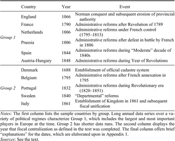
Though fiscal centralization in Europe was a centuries-long process, it remained largely unfinished through most of the 1700s. Profound changes often came with the French Revolution and Napoleon. In many places, therefore, centralization is identifiable as a structural shift that occurred from 1789 to 1815.
A simple definition makes comparisons across polities possible. Fiscal centralization was completed the year that the national government began to secure revenues by way of a tax system with uniform rates throughout the country.Footnote 14 This change typically occurred in the context of large-scale administrative reforms that established new state bureaucracies. Appendix 1 documents the details of fiscal centralization for each polity.
In reality, levels of fragmentation varied across countries. To bias the evidence against my hypothesis, I have classified all pre-centralized regimes as completely fragmented, even for polities where fragmentation was quite low. Thus, the statistical results will be even stronger than I claim if they still indicate that centralized regimes were associated with significantly higher revenues than fragmented ones.
FISCAL CENTRALIZATION IN EUROPE

Notes:
The first column lists the sample countries by group. Long annual data series over a variety of political regimes characterize group 1, which includes the largest and most important players in Europe at the time. Group 2 has shorter data runs. The second column displays the year that fiscal centralization as defined in the text was completed. The final column offers brief “explanations” for the dates, which are elaborated upon in appendix 1.
Sources:
See the text.
Table 1 indicates that fiscal centralization took place swiftly and permanently throughout much of the continent from 1789 onwards.Footnote 15 The National Assembly transformed the tax system in France by eliminating traditional exemptions and privileges. Napoleon completed this process after the coup in 1799.Footnote 16 French conquest of Belgium, the Dutch Republic, and various Italian polities led to significant administrative changes, including tax reform. After defeat in battle by France in 1806, Prussia also made major fiscal innovations.
Some exceptions bear mention. England had centralized institutions from early on. On the other hand, the French failed in their attempts to make administrative changes on the Iberian Peninsula: fiscal centralization in Portugal and Spain did not happen until 1832 and 1844, respectively. The same is true for Austria-Hungary, where fiscal centralization occurred with the Revolutions of 1848. For Scandinavia, I dated fiscal centralization in Denmark to the establishment of the cadastre system in 1688. Significant fiscal change did not occur in Sweden until 1840, however.
From Executive Discretion to Parliamentary Control
Sovereigns retained control over expenditures through the end of the Napoleonic era. Indeed, the consolidation of fiscal powers by national governments may have exacerbated problems of executive discretion. I now discuss the second part of our story: effective constraints that limited the ways in which rulers could spend public funds.
Consider, for example, what happened in the Netherlands. The 1815 constitution granted absolutist powers to King Willem I (1815–1840).Footnote 17 Parliamentary budget authority, which came at ten-year intervals, was rendered ineffective. Spending heavily on the military, on infrastructure, and on the monarchy itself, Willem could not balance the national accounts. Though fiscal centralization roughly doubled the size of the Dutch tax base and Europe was politically stable, public debt increased to more than 200 percent of GDP—a ratio comparable to that during the Revolutionary and Napoleonic Wars—under his reign. The king also used semi-legal means to hide the true state of government finances. When Willem's fiscal troubles finally became public in 1839, parliament vetoed the upcoming decadal budget and the king abdicated his throne. The constitutional amendment passed in 1840, replaced the ten-year budgets with two-year ones, and made information about state finances readily available. A new constitution, promulgated during the Year of Revolutions in 1848, marked the establishment of a truly liberal era in the Netherlands. From that point onwards, the crown had to submit annual budgets to parliament for approval. By instituting a firm check on executive spending, the reform of 1848 became—in the words of Jan Luiten Van Zanden and Arthur Van Riel—the cornerstone of parliamentary power.Footnote 18
Though monarchs spent revenues as they wished, representative bodies exercised tax authority. As the well-known example of King Charles I (1625–1649) of England demonstrates, rulers hoped to evade parliament in the search for greater funds. Forced loans, repaid in highly unpredictable ways and in terms altered from original agreements, were one major revenue stream for Charles. The king also seized private goods such as bullion. Other measures to skirt parliament included customs impositions and the sale of monopolies, government lands, and offices. Charles, moreover, kept parliament in the dark about the state of public finances.Footnote 19 Such predatory fiscal tactics by English monarchs continued until the Glorious Revolution.
Absolutists thus found themselves locked in a vicious circle. Parliaments rightfully feared that kings would spend additional revenues in reckless ways. They therefore demanded limits as a precondition before providing new funds. Yet because parliaments were unwilling to bend, rulers often resorted to fiscal predation. This misbehavior, of course, only reinforced the notion that executives could not be trusted. In turn, parliaments fervently resisted tax requests and revenues remained low.
Limited government, which generally emerged during the nineteenth century, established parliament's power of the purse. Parliamentary control of national budgets reduced the likelihood of poor spending choices by rulers. Just as they each had reasons (as in Hoffman and Rosenthal) to favor fiscal centralization, both executives and parliaments had incentives to establish limits. Centralization meant that monarchs would receive greater funds. Surrender of budgetary control was the only credible way for crowns to guarantee that a portion of new revenues would go towards desired public services. So long as executive and parliament reached a deal, regimes with low levels of taxation and spending were less attractive.Footnote 20
Hoffman and Rosenthal claim that limited government arose after 1800 because of an important change in the nature of warfare. For the first time, leaders who failed in battle also faced the risk of losing their thrones. Thus, the benefits of higher tax revenues that rulers could use to wage war began to outweigh the advantages of absolute control over expenditures. As Daron Acemoglu and James Robinson argue, rulers may have also gained from nonmilitary forms of spending such as the provision of public services or redistribution that prevented social unrest.Footnote 21
Timing is the key difference between Hoffman and Rosenthal's argument and mine. The authors suggest that fiscal centralization and limited government occurred in one fell swoop. My dating scheme, however, indicates that the two transformations happened in chronological order. Though centralization and limited government were interdependent shifts, it was not until decades after centralization—which was in many cases imposed “exogenously” by the French—that stable limited government regimes were established.
One obvious reason for this disparity lies in the divergent aims of the two studies. Hoffman and Rosenthal wish to explain the broad shift from absolutist regimes to parliamentary ones. It is thus useful to consider centralization and limited government as dual parts of a single simultaneous change. My intent, by contrast, is to perform a statistical analysis that unites various arguments about the importance of political transformations. Selection of the “right” dates matters because a choice that is too early or too late may lead to false acceptance or rejection of the relevant hypotheses. Hence, it is imperative to identify the precise years in which centralized as well as limited regimes were first established.
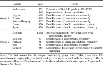
Since budget authority increased over time, a reasonable portrayal of limited government must capture parliament's real power to act. It should also be simple enough to apply to all sample countries. My definition harkens back to the spirit of constitutional reform as expressed by North and Weingast. Limited government emerged the year in which parliament gained the stable constitutional right to control the national budget on an annual basis. For stability, parliament's power of the purse had to hold for at least two consecutive decades. So that dating is as objective as possible, I have chosen years and regimes for which there is widespread consensus. The coding of limited regimes corresponds closely to the classification systems used by Charles Tilly, Bradford De Long and Andrei Shleifer, Acemoglu, Simon Johnson, and Robinson, and Keith Jaggers and Monty Marshall.Footnote 22 Incorporation of these three factors—a regular veto right by parliament over the budget, regime stability, and scholarly agreement—means that political arrangements were classified as limited in a manner that closely resembles the standard put forth by North and Weingast for England.Footnote 23 Appendix 1 documents the details of limited government for each country.
To bias the evidence against my hypothesis, I have always selected an early date to define political regimes as limited. This choice means that average revenues associated with limited government will be lower than otherwise. For the sake of argument, say that limited government did not “truly” emerge in Germany until after World War II and in Spain until after Franco's death in 1975. If so, then the correct method would be to categorize pre-twentieth-century Prussian and Spanish data as absolutist and post-twentieth-century data as limited. Since public revenues in Europe have grown over time, this classification scheme would only strengthen any results that limited regimes were associated with revenue increases.
Limited government was occasionally shaky during the 1800s. Recall that my definition sets a minimum threshold for stability by requiring that parliament's constitutional rights held for at least 20 straight years. It would be impractical to demand that limited government was a “permanent” reform. Moreover, as discussed above, pushing back the years for limited government in this way would likely reinforce any findings that executive constraints improved public finances. In the regression analysis, I also allowed for uncertainty over how long new limited regimes would last by including five-year or ten-year lags on their start dates as a robustness check.
I now present a case study of France to illustrate my dating methodology. Established after Napoleon's final defeat in 1815, the Bourbon regime was limited in name only. Over the next several years, there were intense battles between royal and liberal forces. The notion of proper governance of Charles X, who acceded to the throne at the start of the 1820s, was hardly compatible with constitutional monarchy. In 1830 he dissolved parliament, reduced the electorate in favor of the wealthy, placed the press under government control, and called for new elections—measures that incited the July Revolution the next day. Louis Phillippe, who replaced the deposed king, agreed to adhere to constitutional limits, but because his reign ended in revolution in 1848—and thus lasted for less than two decades—I did not classify it as limited. One of the robustness checks, however, categorized it as such. In 1851 Napoleon III mounted a coup d'etat and established an authoritarian regime that lasted nearly 20 years. The Third French Republic, founded in 1870, remained until the German invasion of 1940.Footnote 24 Since this final arrangement best satisfied the triple criteria of regularity, stability, and consensus, I dated the emergence of a limited regime in France to 1870.
LIMITED GOVERNMENT IN EUROPE

Notes:
The first column lists the sample countries by group, which table 1 describes. The second column displays the year that limited government as defined in the text emerged. The final column offers brief “explanations” for the dates, which are elaborated upon in appendix 1.
Sources:
See the text.
In Europe as a whole (as table 2 indicates), limited government reforms began during the 1830s and 1840s, several decades after centralization. A second wave of limited government reforms occurred in the 1860s and 1870s. England, however, was precocious since limits on executive spending emerged nearly 150 years earlier. At the other extreme, Denmark did not establish a stable constitutional monarchy before World War I.
Political risks and instability dominated the Iberian Peninsula during the nineteenth century. Thus, “liberal” regimes there fit less well with traditional notions of limited government. I have dated a limited regime in Portugal to 1851 and in Spain to 1876. Since Iberian revenues remained low through the 1800s, this choice biases against the hypothesis that constitutional constraints mattered. Classification of the Iberian regimes as absolutist would only strengthen any findings that limited government was associated with improvements in public finances.
Implications for Public Finances
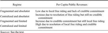
Table 3 provides a summary of the public finance characteristics of the four possible political regimes: fragmented and absolutist, centralized and absolutist, fragmented and limited, and centralized and limited. Note that there was only one example of a fragmented and
PUBLIC FINANCE CHARACTERISTICS OF POLITICAL REGIMES

Sources:
See the text.
limited regime among sample countries.Footnote 25 Revenues under centralized and limited regimes should have been higher than under fragmented and absolutist ones. Fiscal centralization implied an increase in revenues over fragmentation because it eliminated local free riding. Similarly, limited government implied an increase in revenues over absolutism. Parliaments were more willing to submit to tax requests since rulers could make credible commitments to spend funds on public services rather than personal consumption.
By the same logic, revenues should have increased under centralized and absolutist regimes in comparison with fragmented and absolutist ones. They should have also been higher under fragmented and limited regimes than under fragmented and absolutist ones. Finally, revenues under centralized and limited regimes should have highest of all since both sorts of fiscal problems had been resolved.
REVENUE DATA AND SAMPLE COUNTRIES
I assembled a database on annual revenues and population from many secondary sources. Chief among them were Bonney's European State Finance Database (ESFDB) for the seventeenth and eighteenth centuries and Brian Mitchell's International Historical Statistics (IHS) for the nineteenth and early twentieth centuries. Appendix 2 documents the data sources and construction methods for each sample country.
The historical data had certain limitations. Since European countries did not maintain detailed financial records during the seventeenth and eighteenth centuries, the time series may be imprecise. Bonney shows that governments may have calculated annual revenues in several different ways.Footnote 26 I have done my best to stick to income from tax receipts for a given year. When feasible, ordinary and extraordinary figures were added together and loan income was subtracted in order to determine total revenues. Since the various ways in which monarchs tabulated annual revenue streams prior to the 1800s suggest that they typically overestimated the amount of financial resources available to them, average revenues associated with fragmented and absolutist regimes should be larger than otherwise. In turn, the empirical framework biases against the hypotheses that fiscal centralization and limited government were associated with significant revenue increases.
The revenue data also came in different currencies. To make calculations comparable across countries, I transformed all units into grams of gold. In addition, some observations were missing. Those years were linearly interpolated. Since most instances of fiscal change save centralization during the Revolutionary and Napoleonic times were gradual, interpolations should provide reasonable estimates. I interpolated population data between census years as well. Since major population shocks such as plague did not occur for the period under consideration, the previous logic also applies.
I have divided the sample into two groups based on data availability and historical importance. Annual published series of nearly two centuries or more for revenues as well as a variety of controls typically exist for the six polities (Austria-Hungary, England, France, the Netherlands, Prussia, and Spain) that comprise the first group. These countries were among the largest and most powerful players in Western Europe at the time, and for them data were available over a variety of political regimes.Footnote 27
Shorter published time series exist for the five countries (Belgium, Denmark, Italy, Portugal, and Sweden) in the second group. Revenue data for Belgium and Italy only began after they were founded as constitutional monarchies in 1831 and 1861, respectively. Annual series for Portugal and Sweden did not start until after the establishment of centralized and limited regimes during the 1800s.Footnote 28 Denmark never
SUMMARY STATISTICS OF PER CAPITA REVENUE DATA (in grams of gold)

Source:
See appendix 2.
achieved a stable form of limited government by 1913. It thus functioned as an additional “absolutist” control in the regressions.Footnote 29 Data prior to political transformations was not available for the second set of countries. Despite these limitations, including these countries enriches the sample by expanding the range of institutional experiences.
POLITICAL REGIMES AND PUBLIC REVENUES
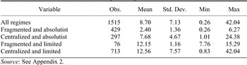
Table 4 displays the summary statistics for the revenue panel. In total, there are 1,515 observations, 429 for fragmented and absolutist regimes, 297 for centralized and absolutist ones, and 713 for centralized and limited ones.Footnote 30 Seventy-six observations characterize the lone fragmented and limited regime. What jumps out is the large average per capita revenues associated with centralized and absolutist regimes (7.68 grams of gold) and centralized and limited ones (12.56 grams of gold) relative to those of fragmented and absolutist ones (2.40 grams of gold). Per capita revenues for the fragmented and limited regime (12.15 grams of gold) are also significantly higher.
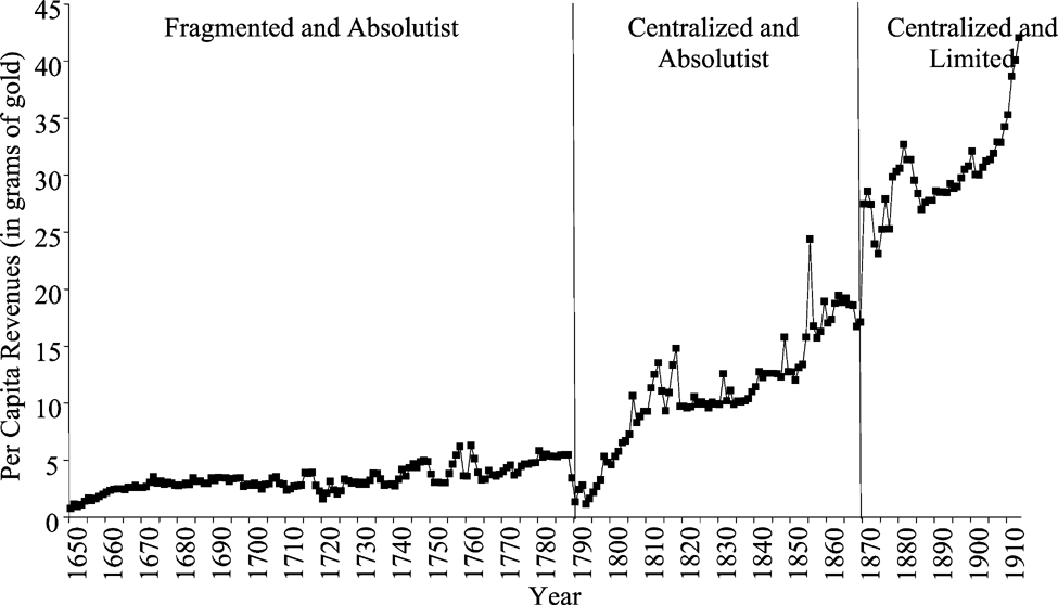
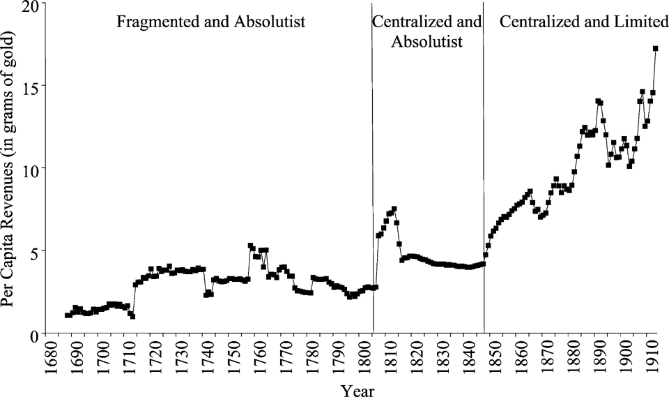
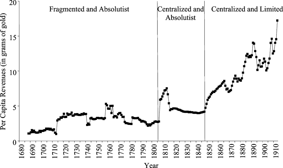
Before moving on to the statistical analysis, it is worthwhile to study France and the Netherlands, two sample polities for which long runs of data are available. Figure 1, which plots annual per capita revenues over political regimes in France from 1650 to 1913, indicates that revenues remained low at less than 5 grams of gold per capita under the fragmented and absolutist regime that lasted through the 1780s. The French Revolution (1789–1799) led to the establishment of a national tax system. Coinciding in time with the Revolutionary and Napoleonic wars, we observe a sharp increase in revenues through 1815, which doubled to approximately 10 grams of gold per head. Over the next two decades, French revenues leveled out but never fell. Revenues again began to increase in the 1840s—albeit at a slower rate than during Napoleonic times—to almost 20 grams of gold per capita by the end of the 1860s.Footnote 31 With the establishment of a centralized and limited regime in 1870, we observe another sharp increase in revenues, which doubled over the next four decades to 40 grams of gold per head by the start of World War I.Footnote 32
YEARLY PER CAPITA REVENUES, FRANCE, 1650–1913

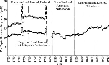
The Dutch Republic (1572–1795) was unique among sample countries in that each of its seven provinces had separate systems of administration, representation, and taxation. The fragmented nature of fiscal institutions at the national level contrasted with those in Holland, the wealthiest and most heavily populated province, where the local government established a centralized tax system in 1574 by extending common taxes from urban areas to rural ones. In turn, the province reduced local free riding and greatly increased its collection of per capita revenues.Footnote 33
The Dutch case well illustrates why it is difficult to draw meaningful distinctions between the terms “limited” and “absolutist” before the nineteenth century. Though typically considered “constitutional,” the republic was not limited in the sense of a parliament that monitored executive spending.Footnote 34 I have designated the national political regime in the Dutch Republic as fragmented and limited and the provincial one in Holland as centralized and limited.Footnote 35
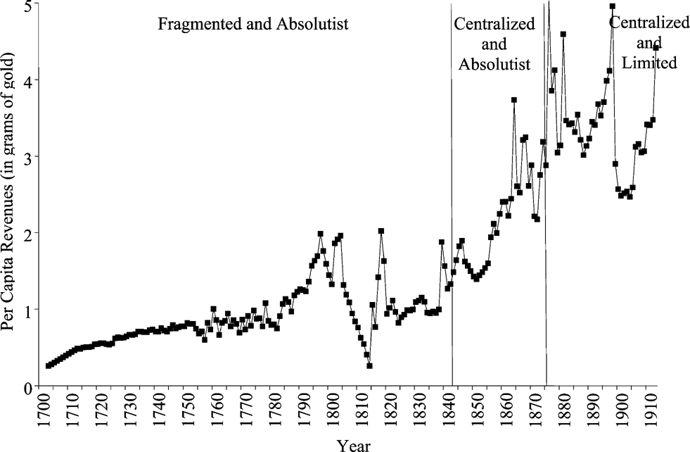
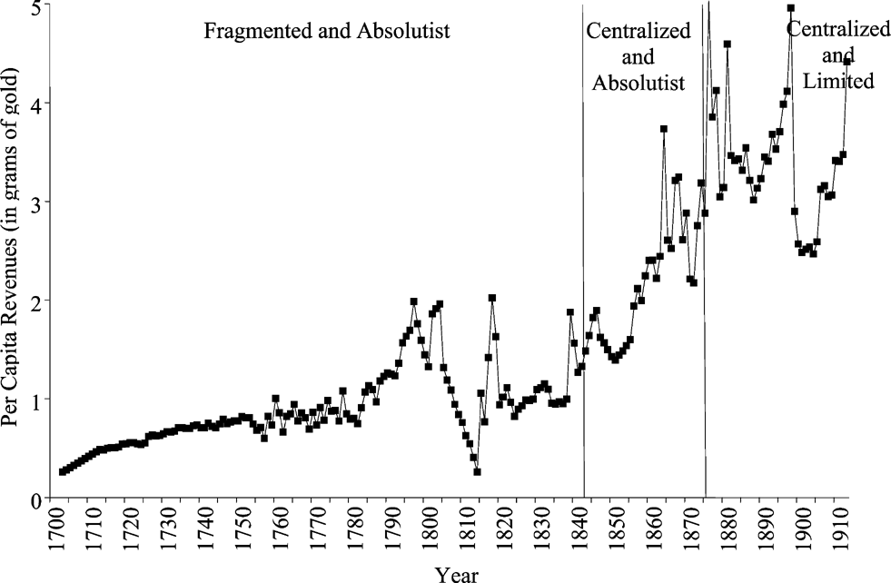
Figure 2 plots annual per capita revenues over political regimes in the Netherlands from 1719 to 1913. The results are consistent with the notion that the republic benefited from its constitution. In the eighteenth century, federal revenues exceeded those in absolutist France by around 5 to 7 grams of gold per head per year. For the 1700s, I also constructed a separate revenue series for centralized Holland. Comparison with the fragmented federal regime reveals a striking difference: per capita revenues in Holland were around 5 to 8 grams of gold higher each year.Footnote 36
Fiscal centralization occurred at the national level in 1806. The Kingdom of the United Netherlands, which emerged at the end of the Napoleonic era, invested King Willem I with absolutist powers. The move to absolutism appears to have offset any gains from centralization. Though Wantje Fritschy notes a 20 percent increase in revenues after 1806, figure 2 suggests that per capita revenues over the length of the absolutist regime were 2 to 6 grams of gold lower than in the pre-1795 Republic.Footnote 37 Comparison with eighteenth-century Holland indicates that revenues under the absolutist regime fell by half.Footnote 38 The revolutions of 1848 saw the establishment of a centralized and limited regime throughout the Netherlands. In turn, Dutch revenues grew steadily, reaching approximately 15 grams per capita by the 1870s. This level resembled that of the centralized and limited regime in Holland one hundred years before.Footnote 39
YEARLY PER CAPITA REVENUES, NETHERLANDS, 1720–1913

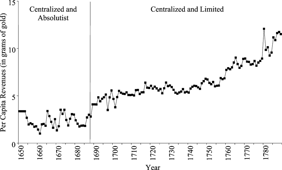
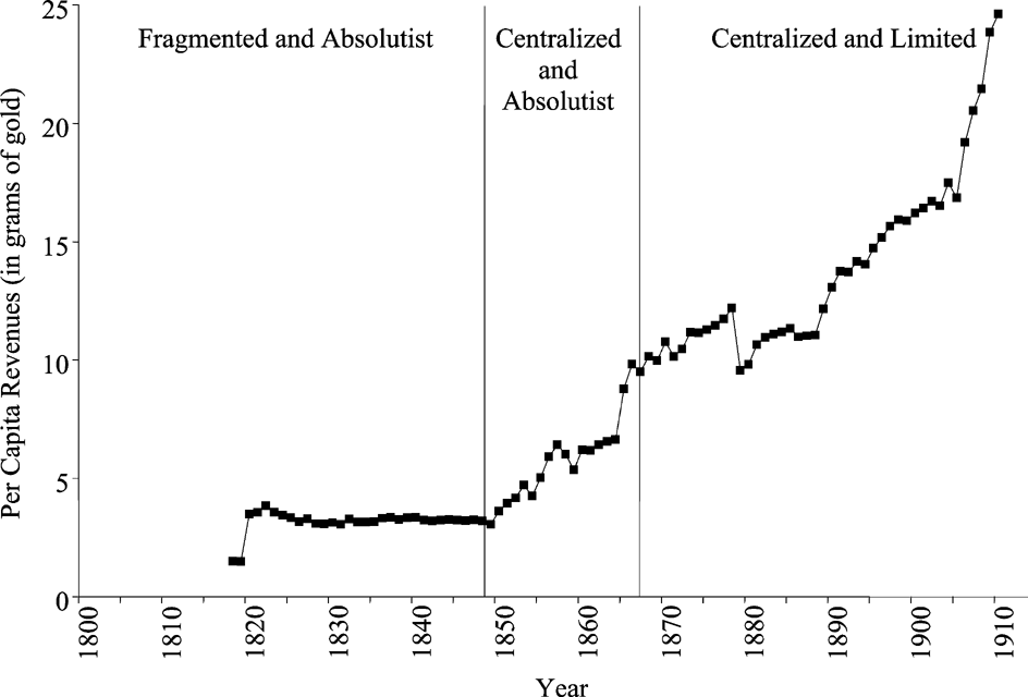
To supplement the case studies, it is useful to examine the rest of the data. Figures 3 through 6 plot annual per capita revenues over political regimes for other group 1 countries. English revenues nearly doubled in the years that followed the establishment of limited government in 1688. Considerable revenue increases were associated with fiscal centralization and limited government in Austria-Hungary, Prussia, and Spain as well.
YEARLY PER CAPITA REVENUES, BRITAIN, 1650–1789

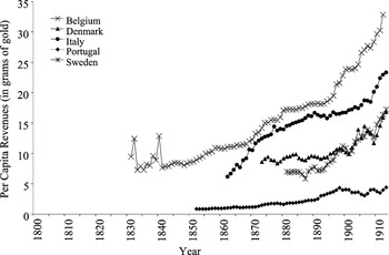
The group 1 evidence suggests that fundamental changes in political structures improved public finances. It is not definitive, however. Figure 7, which plots annual per capita revenues for group 2 countries from 1800 to 1913, highlights the importance of controls for factors besides political institutions. The smallest revenue streams were associated with the limited regime in Portugal. Though limited regimes in Belgium and Italy performed markedly better than the absolutist one in Denmark, there was no clear difference in revenue levels between the Danish regime and its limited counterpart in Sweden. To account for economic, geographic, institutional, and political effects, I now turn to a more rigorous quantitative analysis.
ESTIMATING THE EFFECT OF POLITICAL REGIMES
Panel Regressions
Estimations of panel data increase informative content by combining variations across time and country. There are three econometric concerns particular to this sort of data: contemporaneously correlated errors, panel heteroskedasticity, and serial correlation. One technique that corrects for such problems is feasible generalized least squares (FGLS). FGLS is “feasible” because it employs an estimate of an unknown error process. However, Nathaniel Beck and Jonathan Katz show that this approach often leads to poor estimates of standard errors.Footnote 40 They suggest the use of ordinary least squares with “panel-corrected” standard errors (PCSE) instead. I followed the advice of Beck and Katz and employed PCSE that corrects for contemporaneously correlated errors and panel heteroskedasticity along with a common AR1 term to control for serial correlation.Footnote 41 The fact that OLS is less efficient than FGLS means that the results of the regressions will be stronger if we still find significant coefficients attached to the variables of interest. The FLGS approach, it should be noted, delivered results that were statistically similar if not stronger than those reported.
YEARLY PER CAPITA REVENUES, AUSTRIA-HUNGARY, 1818–1910

YEARLY PER CAPITA REVENUES, PRUSSIA, 1688–1913
The basic fixed effects regression specification is

where Revit is per capita revenue in grams of gold for country i in year t, X is a vector of control variables to be described, and εit is the disturbance term. I used dummy variables for centralized and absolutist (CA), fragmented and limited (FL), and centralized and limited (CL) regimes relative to fragmented and absolutist ones as a clear and simple method to measure the impact of political arrangements on revenues.
Beck claims that well-specified models often do not require fixed effects by unit or time.Footnote 42 Ideally, one wishes to explain effects in terms of substantive variables rather than conclude that revenues were larger in say England simply because it was England. I still chose, however, to include country fixed effects that captured constant but unmeasured economic, geographic, institutional, or political features of individual sovereignties. I did not use yearly fixed effects because in my data set the number of annual observations for group 1 countries typically exceeded 200. Both William Greene and Jeffrey Wooldridge argue that the large cost in terms of lost degrees of freedom makes it difficult to justify yearly fixed effects in such cases.Footnote 43 I did, however, implement time controls that captured widespread shocks such as warfare and changes in the cumulative world stock of gold.Footnote 44
YEARLY PER CAPITA REVENUES, SPAIN, 1703–1913
The effect of military conflict on public finances cannot be overstated. Hoffman and Rosenthal claim that the one true goal of early modern rulers was to wage war for royal glory and homeland defense.Footnote 45 In the 1800s Niall Ferguson argues that political events were more important to investors than economic ones because there was a greater amount of regular information available about them.Footnote 46 One may imagine that revenue levels increased during conflicts themselves but fell just afterwards. The previous authors claim that the total effect of warfare on public finances was negative due to the destruction that it caused. Charles Tilly, Hoffman and Norberg, Epstein, Patrick O'Brien, Rosenthal and R. Bin Wong, and others, however, argue that over the long run, military competition fostered financial innovations that allowed sovereigns to raise larger tax amounts.Footnote 47 Structural changes would suggest that revenues remained permanently higher after war's end. Whether a country won or lost a conflict also influenced revenue levels. So long as the defeated country took more casualties, then the reduction in its tax base would have been more severe.
YEARLY PER CAPITA REVENUES, GROUP 2 COUNTRIES, 1800–1913

Not all conflicts were created equal, however. Two important characteristics were the strength of the enemy and the scope of the war. An ideal measure of opponent size would be total revenues and expenditures. Unfortunately, this approach suffers from endogeneity. One may envision an “arms race,” where the home country repeatedly ratcheted up wartime revenues (and so expenditures) to counteract sequential increases by its adversaries. Debt figures would also be useful to assess the pressure of warfare on public finances, but continuous series were not available. To proxy for debt overhang, one could employ the military's share of total expenditures at war's end. As Hoffman and Rosenthal point out, however, warfare was by far the largest component of national budgets through the nineteenth century.Footnote 48 Thus, military size as well as total expenditures fell rapidly in the years just after wars.
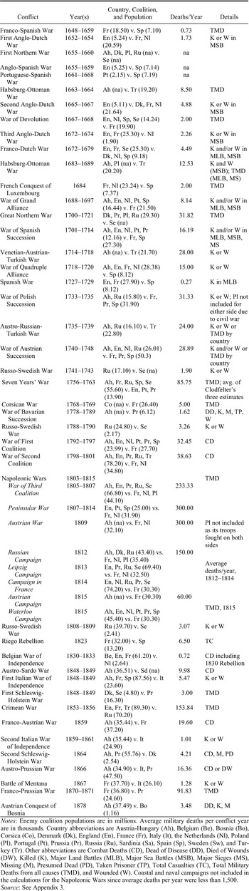
To evaluate the impact of warfare on public revenues, I constructed a new data set based on Micheal Clodfelter.Footnote 49 Appendix 3 documents the details. I included all conflicts fought at least in part in Western Europe (as well as those fought at least in part in Eastern Europe so long as they involved at least one sample country) from 1650 to 1913. I used coalition populations as simple measures of opponent strength that avoided endogeneity problems. Totals were computed as sums of available populations of coalition countries in the years that conflicts began. To gauge the scope of war, I calculated average military deaths per conflict year.Footnote 50 In certain years, sample countries were involved in two or more wars. Both (i.e., nonoverlapping) coalition totals and average deaths were summed in such cases.
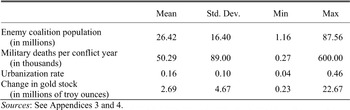
Table 5 summarizes the control variables. The average conflict involved coalition populations of more than 25 million and 50,000 military deaths per year. The smallest coalition (1.16 million) was comprised of Bosnia and Herzegovina during the conquest by Austria-Hungary in 1878. The largest (87.56 million) was comprised of the combined populations for Austria-Hungary, France, and Spain during the First Italian War of Independence from 1848 to 1849. The least deadly conflict was the Spanish War from 1727 to 1729, with 269 military deaths per annum. The deadliest single year occurred in 1809, when military deaths for the Peninsular and Austrian fronts of the Napoleonic Wars totaled 600,000.
SUMMARY STATISTICS OF CONTROL VARIABLES

Sources:
See appendices 3 and 4.
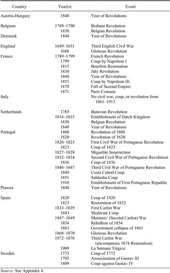
We must also consider the impact of domestic turmoil. One may expect that internal chaos caused disruptions that reduced revenue flows. To measure this effect, I assembled a data set identifying all civil wars, coups, and revolutions that occurred within sample countries from 1650 to 1913. Appendix 4 provides the details. In the regression analysis, I included a dummy variable that took a value of one for each year of internal conflict.
One may suppose that economic growth increased tax bases and enabled sovereign governments to collect larger revenues as well. Since reliable GDP figures are difficult to come by before 1820, many studies of the late nineteenth century employ measures of foreign trade as approximates of national output.Footnote 51 However, systematic trade deficit and export series from the 1600s onwards were not available. Paul Hohenberg and Lynn Lees, Paul Bairoch, and Acemoglu et al. argue that there was a close relationship between urbanization rates and income growth.Footnote 52 To proxy for per capita GDP, I constructed a yearly variable that calculated urban populations as fractions of total populations for each country. Appendix 4 describes the details.Footnote 53 Note that controls for national income also helped account for different rates of technological innovation and adoption across countries.Footnote 54Table 5 indicates that on average urban populations comprised 16 percent of total populations. The lowest urbanization rates were 4 percent for Prussia during the 1700s and the largest were over 40 percent for England from the 1870s onwards.
Recall that I converted currency units into grams of gold. This transformation should reduce any effects of inflation. Though the world stock of gold remained stable through the start of the nineteenth century, large discoveries in California in 1848 and in Australia in 1851 had a dramatic effect on output.Footnote 55 I employed data from François Velde and Warren Weber to account for annual changes in the cumulative gold stock in millions of troy ounces from 1650 to 1913.Footnote 56Table 5 indicates that the gold stock increased by an average of 2.69 million troy ounces per year. The smallest single year change (230,000 troy ounces) occurred between 1650 and 1651 and the biggest (22.67 million troy ounces) occurred between 1911 and 1912.
The econometric setup assumes that it is possible to disentangle political regimes from factors such as violent conflicts and economic fundamentals. Since political arrangements influenced all of these characteristics, coefficients on the control variables rather than those on the regime ones themselves may capture some of the positive effects of institutional reforms. Hence, regime coefficients likely underestimate the total impact of political arrangements on public revenues.
Structural Breaks
Structural breaks tests, which assume no a priori knowledge of major turning points in the revenue series, are another relevant technique. By allowing the data to “speak” for themselves, breaks tests offer a useful alternative to standard regression analysis.Footnote 57 I use the methodology proposed by Jushan Bai and Pierre Perron that identifies multiple structural changes in means while allowing for serial correlation.Footnote 58 It thus improves upon the “moving windows” technique that relies upon sequential single structural change methods. Since I am interested in turning points associated with political transformations, I apply the method to Group 1 countries only.
A program created for the Regression Analysis of Time Series (RATS) software performs the Bai-Perron procedure, which considers the following regression for each sample polity in Group 1

where Revt is per capita revenue in grams of gold in year t, β0 and β1 through βL are parameters to be estimated, and εt is the disturbance term. I allowed up to five significant yearly lags l of the dependent variable (L = 5). The RATS routine, which uses a dynamic programming algorithm to evaluate which final partitioning of the time series data achieves a global minimization of the overall sum of squared residuals, returns the optimal set of break points.
The routine calls for the selection of a maximum number of “best” turning points in the time series for each country subject to a minimum number of observations between data segments. As Kristen Willard, Timothy Guinnane, and Harvey Rosen point out, there is always a trade-off in determining parameter values.Footnote 59 A minimum space of two observations eliminates the chance of confounding the effects of different events, but ends up analyzing blips (i.e., false positives that characterize certain events as “long-lasting” that really were not) rather than turning points.Footnote 60 Longer time periods of analysis, however, increase the likelihood of missing important shifts (i.e., false negatives). After some experimentation, I selected the best five breaks from 1650 to 1913 with at least 25 observations (i.e., 25 years) per segment.Footnote 61 As mentioned above, there is a gap in the revenue series for the Netherlands that coincides with the fall of the republic in 1795 and prevents the identification of a turning point associated with fiscal centralization in 1806. I thus chose the best three breaks with at least ten observations (i.e., 10 years) per segment over the nineteenth century, when the Netherlands established parliamentary government. The per capita revenue series for Austria-Hungary, which did not begin until 1818, required similar parameters. For robustness, I also applied this framework to the other group 1 countries (France, Prussia, and Spain) that experienced political transitions during the 1800s.
STATISTICAL EVIDENCE
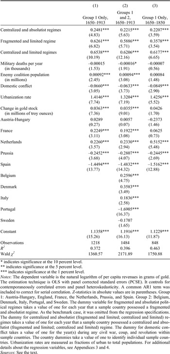
Table 6, which displays the results of regression 1, reveals that fragmented and absolutist regimes collected significantly less revenue per capita than any of the other regime types. The findings held for both group 1 countries only (column 1) and when group 2 countries were included (column 2).Footnote 62Ceteris paribus, the move to a centralized and absolutist regime increased revenues by 22 to 25 percent, the move to
REGRESSION RESULTS FOR POLITICAL REGIMES AND PUBLIC REVENUES

* indicates significance at the 10 percent level.
** indicates significance at the 5 percent level.
*** indicates significance at the 1 percent level.
Notes:
The dependent variable is the natural logarithm of per capita revenues in grams of gold. The estimation technique is OLS with panel corrected standard errors (PCSE). It controls for contemporaneously correlated errors and panel heteroskedasticity. A common AR1 term was included to correct for serial correlation. Z-statistics in absolute values are in parentheses. Group 1: Austria-Hungary, England, France, the Netherlands, Prussia, and Spain. Group 2: Belgium, Denmark, Italy, Portugal, and Sweden. The dummy variable for fragmented and absolutist political regimes takes a value of one for each year that a sample country possessed a fragmented and absolutist regime. As the benchmark case, it was omitted from the regression specifications. The dummy for centralized and absolutist (fragmented and limited; centralized and limited) regimes takes a value of one for each year that a sample country possessed a centralized and absolutist (fragmented and limited; centralized and limited) regime. The dummy for domestic conflict takes a value of one for the year(s) during any civil war, coup, and revolution within sample countries. The country dummies take a value of one to identify individual sample countries. Urbanization rates are measured as fractions of urban to total populations. For additional details about the regression variables, see appendices 3 and 4.
Sources:
See the text.
the fragmented and limited one by 59 to 63 percent, and the move to a centralized and limited one by 62 to 65 percent.Footnote 63 Specifications with gross revenues as the dependent variable and population, urbanization rates, and a population-urbanization interaction term as independent variables delivered results statistically similar to those reported. The findings were also robust to checks that eliminated any “abnormal” observations and used alternative regime classifications as described before.Footnote 64
What about the control variables? The destruction that warfare caused as measured by average military deaths per conflict year had a small negative effect on per capita revenues. Opponent size as proxied by coalition populations, however, had a significant positive effect. The results suggest that national governments responded to enemy strength: a country that faced the largest recorded coalition (82.5 million) rather than the smallest one (2.15 million) would have increased revenues by around 7 percent.Footnote 65 Domestic turmoil (civil wars, coups, and revolutions) led to a significant reduction in revenues (6 to 7 percent lower than during periods of internal peace). Economic growth (as proxied by urbanization rates) had a significant positive impact.Footnote 66 A country with the largest recorded urbanization rate (0.49) rather than the smallest one (0.04) would have increased revenues by around 60 percent. The effect of changes in the cumulative world gold stock was also significant. A per year increase of one million troy ounces led to a 4 percent increase in revenues. France (19 to 22 percent higher) and the Netherlands (23 percent higher) had much larger revenues per head than England, as did Belgium (26 percent higher), Denmark (36 percent higher), and Italy (18 percent higher) among group 2 countries. Prussia (25 to 28 percent lower) and Spain (145 to 148 percent lower), on the other hand, had much smaller per capita revenues than England, as did Portugal (169 percent lower) among Group 2 countries.
Before moving to the structural breaks, it is useful to take a second look at the impact of economic growth. Joel Mokyr characterizes the Industrial Revolution in two phases. The first occurred in Britain from roughly 1750 to 1825. The second occurred in Western Europe and North America from roughly 1850 to 1913.Footnote 67 Though limited government was established in England prior to phase one, it typically emerged on the continent during or after the start of phase two.
Recall that I have controlled for income effects in the regressions by including urbanization rates as an independent variable. To reduce the impact of the second Industrial Revolution, I also ran the same set of regressions on group 1 countries for the period before 1850. As column 3 of table 6 shows, political transformations towards centralized and limited regimes continued to be associated with significant increases in per capita revenues.Footnote 68
A brief review of the transformations that occurred prior to the nineteenth century also proves helpful. Recall that per capita revenues increased quickly in the years that followed fiscal centralization in France in 1790 (figure 1). In addition, a second glance at the Dutch case indicates that revenues in centralized Holland were a great deal larger than in the fragmented republic as a whole (figure 2). Finally, we observe a significant increase in revenues after the establishment of limited government in England in 1688 (figure 3). The pre-1800 evidence thus suggests that political regimes had important effects on public revenues independent of economic growth associated with the Industrial Revolution.
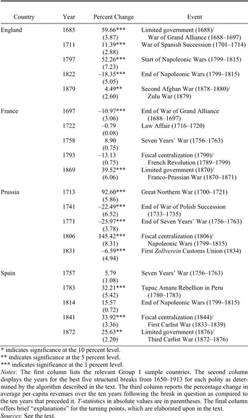
Table 7, which displays the results of the structural breaks tests described in equation 2 from 1650 to 1913, reveals close relationships
MAJOR BREAKS IN PER CAPITA REVENUE SERIES, 1650–1913

* indicates significance at the 10 percent level.
** indicates significance at the 5 percent level.
*** indicates significance at the 1 percent level.
Notes:
The first column lists the relevant group 1 sample countries. The second column displays the years for the best five structural breaks from 1650–1913 for each polity as determined by the algorithm described in the text. The third column reports the percentage change in average per capita revenues over the ten years following the break in question as compared to the ten years that preceded it. T-statistics in absolute values are in parentheses. The final column offers brief “explanations” for the turning points, which are elaborated upon in the text.
Sources:
See the text.
between major turning points and political transformations that enhanced public finances. It also highlights the link between those innovations and military competition and conflicts.Footnote 69 In England, the break that occurred in 1685 coincided with the establishment of limited government during the Glorious Revolution as well as the start of the War of the Grand Alliance. This change led to a 60 percent increase in average per capita revenues over the following decade. Other turning points in the English revenue series came with the War of the Spanish Succession (1711), near the start (1797) and end (1822) of the Napoleonic Wars, and with various colonial wars (1880). In France, the best breaks were associated with the end of the War of the Grand Alliance (1697), the Law Affair (1722), the Seven Years' War (1758), fiscal centralization (1793), and limited government (1869). The chaos of the French Revolution (1789–1799) swamped any jump in revenues just after fiscal centralization. Figure 1, however, shows that French revenues grew rapidly by the start of the 1800s. Limited government, which coincided with the Franco-Prussian War, led to a 40 percent increase in revenues. In Spain, we observe turning points with the Seven Years' War (1757), a colonial conflict (1783) that foreshadowed the South American Wars of Independence, the end of the Napoleonic Wars (1814), fiscal centralization (1841), and limited government (1872). Both political transformations, which occurred during times of domestic turmoil or warfare, led to revenue increases of 25 to 35 percent.
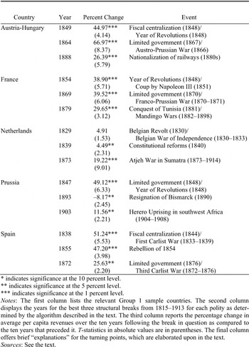
Table 8, which displays the results of the structural breaks tests for the nineteenth century, supports the previous analysis. Limited government (1869) was again a major turning point in the French per capita revenue series. A second break in 1854 followed the Revolution of 1848 and subsequent coup by Napoleon III in 1851. In Spain, two of the three best breaks over the 1800s were associated with political transformations. The turning point in 1838 came near the time of fiscal centralization, while the 1872 break just preceded limited government.
Breaks for Prussia occurred with its entry into the Great Northern War (1713), in the aftermath of the War of the Polish Succession (1741) and the Seven Years' War (1771), with fiscal centralization (1806), and
MAJOR BREAKS IN PER CAPITA REVENUE SERIES OVER THE NINETEENTH CENTURY

* indicates significance at the 10 percent level.
** indicates significance at the 5 percent level.
*** indicates significance at the 1 percent level.
Notes:
The first column lists the relevant group 1 sample countries. The second column displays the years for the best three structural breaks from 1815–1913 for each polity as determined by the algorithm described in the text. The third column reports the percentage change in average per capita revenues over the ten years following the break in question as compared to the ten years that preceded it. T-statistics in absolute values are in parentheses. The final column offers brief “explanations” for the turning points, which are elaborated upon in the text.
Sources:
See the text.
in 1831. Centralization took place the same year as Prussia's disastrous loss to the French at Jena-Auerstedt. That defeat, which prompted significant administrative reforms, led to a 145 percent increase in per capita revenues. It appears that the 1831 turning point was the result of the first Zollverein customs agreement between German polities. The break, which was associated with a 7 percent decrease in revenues, suggests that the elimination of tariffs harmed Prussian finances.
Curiously, limited government—which occurred during the Year of Revolutions in 1848—was not included as one of the best turning points in Prussia from 1650 to 1913. Figure 5, however, shows a substantial increase in per capita revenues from that point onwards. Richard Tilly also argues that constitutional changes sparked by the 1848 Revolution strengthened the government's ability to raise revenues and invest in public infrastructure.Footnote 70 Thus, it was not surprising that the structural breaks tests for the nineteenth century selected 1847 as the best turning point in the Prussian series. According to table 8, limited government boosted revenues by nearly 50 percent.
For the reasons discussed above, the structural analysis for Austria-Hungary and the Netherlands was restricted to the nineteenth century. As table 8 indicates, the best breaks in Austria-Hungary came with fiscal centralization and the Year of Revolutions (1849), limited government and the Austro-Prussian War (1864), and the nationalization of railways that began in the 1880s. Each political transformation led to large revenue increases (45 and 67 percent, respectively). In the Netherlands, we observe turning points with the Belgian Revolt and subsequent War of Independence at the start of the 1830s, the constitutional amendments of 1840, and the start of the Atjeh War in Sumatra in 1873. Interestingly, the break most closely identified with limited government was the abdication of King Willem I and related constitutional reforms at the start of the 1840s, and not the Revolution of 1848. This turning point highlights the importance of the first set of liberal changes, which led to a significant increase in per capita revenues.
CONCLUSION
This article analyzes the relationship between political regimes and public revenues in European countries from 1650 to 1913. Panel regressions indicate that centralized and limited regimes were associated with significant increases in per capita revenues relative to fragmented and absolutist ones. Structural breaks tests that assume no a priori knowledge of possible turning points in the revenue series support these conclusions.
The results lend new credence to arguments that espouse the virtues of limited government. Yet they also suggest that, while a credible commitment to sound fiscal policies is necessary to improve public finances, it is not sufficient. Nascent states in Europe were weak and fragmentation created many headaches. Fiscal centralization—so my analysis suggests—was just as essential as limited government to develop efficient systems of taxation. Indeed, an intriguing topic for future work would be a quantitative study of the effects of tax variations and free riding within Old Regime polities.
Appendix 1: Political Regimes
Fiscal centralization was completed the year that the national government began to secure revenues by way of a tax system with uniform rates throughout the country. Limited government emerged the year in which parliament gained the stable constitutional right to control the national budget on an annual basis. For stability, parliament's power of the purse had to hold for at least two consecutive decades. For additional details, see the text.
Austria-Hungary
Though Napoleon defeated Austria-Hungary in 1805, he was unable to replace Old Regime fiscal structures there. In 1848 a liberal revolution failed. This event, however, was the catalyst for the creation of uniform administrative structures within the Austrian Empire. Most significantly, the central government began to implement an effective Cisleithanian-style tax system in Hungary. I thus date fiscal centralization to 1848. The “Compromise” of 1867, which established Austria and Hungary as distinct political entities, marked the start of a constitutional era. From that point on, both territories had parliaments that exercised regular control over state finances.Footnote 71
Belgium
The First French Republic invaded and annexed Belgium in 1795. Thereafter, fiscal centralization proceeded under Napoleon as for the rest of France. In 1830 Belgium—then part of the Kingdom of the United Netherlands, established at the Napoleonic era's end—declared independence from Dutch rule. Founded as a constitutional monarchy, Belgium became an independent country in 1831.Footnote 72
Denmark
A cadastre system, established for land taxation in 1688, remained in force until the introduction of a modern land tax in 1903. With few exceptions, rates were uniform outside of chartered towns. I thereby date fiscal centralization to 1688 as the best fit with my definition.Footnote 73 In 1848 King Frederick VII declared himself a constitutional monarch. A liberal constitution took effect the following year. However, the 1848 regime endured for less than two decades. Absolutism was restored in 1866. The revised constitution, which allowed the crown to appoint one-fourth of parliament's members, remained in force until 1915.Footnote 74
England (Britain)
By the end of the twelfth century, England had strong national institutions.Footnote 75 I date fiscal centralization to the Norman Conquest (1066), which undercut provincial authority and contributed to the establishment of uniform rule. The Glorious Revolution (1688) established parliament's power of the purse. For references, see the section, “Introduction.”
France
For details, see the text.
Italy
“Italy” was a geographical rather than political expression through the nineteenth century.Footnote 76 Italian polities were typically fragmented. In Piedmont, for instance, the monarch ruled separately over the duchies of Savoy, Aosta, Saluzzo, Monferrat, the principalities of Oneglia and Piedmont, the county of Nice, and later the Kingdom of Sardinia.Footnote 77 Napoleon carried out administrative reforms including fiscal centralization at the start of the 1800s. Bids to enact liberal constitutions in 1848 in Naples and the Papal States failed. King Carlo Alberto of Piedmont, however, was able to establish a constitutional monarchy, which later formed the political basis for the Kingdom of Italy, founded in 1861. The unification of public finances also occurred during this period.Footnote 78
The Netherlands
For details, see the text.
Portugal
Though Napoleon invaded Portugal in 1807, he was unable to implement major economic and political reforms. Comprehensive changes including fiscal centralization did not occur until 1832. In 1820 a liberal revolution failed. The Revolutionary era, which lasted for 31 years, ended with the establishment of a stable constitutional monarchy in 1851.Footnote 79 For a list of nineteenth-century Portuguese revolutions, coups, and civil wars, see appendix 4.
Prussia
After French defeat in the Battle of Jena-Auerstedt in 1806, the Prussian government made quick economic and political reforms including fiscal centralization.Footnote 80 King Freidrich Wilhelm IV endorsed a liberal constitution during the Year of Revolutions (1848). According to R. Tilly, Prussian executives faced binding constraints from that point onwards.Footnote 81 Nonetheless, the fledgling constitutional regime had its shortcomings. In the 1860s, for example, the government operated without legislative approval of the military budget.Footnote 82
Spain
At the start of the 1700s, Bourbon reformers strengthened the power of the crown in Castile and imposed new taxes on Spain's eastern provinces. Tax rates varied across regions, however, depending upon the particular bargain made. I thus take the Bourbon reforms as an example of tax particularism rather than fiscal centralization. For additional details, see the text. Though Napoleon invaded Spain in 1808, the French were unable to generate modern laws and administrative practices. Fiscal centralization did not occur until 1844 amidst a “moderate” decade of institutional reforms. From 1808 to 1876, civil strife created political chaos. After decades of failed initiatives, a stable constitutional monarchy was established in 1876, which lasted until a coup in 1923.Footnote 83 For a list of nineteenth-century Spanish revolutions, coups, and civil wars, see appendix 4.
Sweden
An anachronistic tax system remained in Sweden through the mid-1800s. I date fiscal centralization to the far-ranging “departmental” reforms of 1840 that strengthened the central government.Footnote 84 The constitution of 1809, intended to limit the executive's power, failed to bring fundamental change. The king retained absolute veto authority and parliament met only once each five years. Sweden remained conservative through the 1860s. I date limited government to 1866, when Prime Minister De Greer led a successful effort to dissolve the Diet of Estates and introduce a bicameral legislature.Footnote 85
Appendix 2: Sources for Revenue Data
Revenue figures concern income from taxation collected by national governments. Loan income was subtracted whenever possible. I use abbreviations to denote different series for revenue (REV1, REV2…) and population (POP1, POP2…). Other abbreviations are Mitchell's British Historical Statistics (BHS) and International Historical Statistics (IHS). The complete data set is available at the Global Price and Income History Group's website at http://gpih.ucdavis.edu/. For additional details, see the text.
Austria-Hungary
REV1 is central government revenue in Austria, 1781–1913, from Mitchell, IHS. The series covers Austria-Hungary through 1847 and from 1850–1867 and Cisleithania only (i.e., the Austrian portion) for 1848/49 and from 1868 onwards. Lombardy is included through 1858 and Venetia through 1865. Total yields are for fiscal receipts only to 1864 and ordinary receipts from 1865–1875. From 1876 onwards, they include certain extraordinary receipts. From 1875–1890, the Mitchell data include cash saldi and loan proceeds. Hence, for those years I used corrected figures (i.e., without saldi or loan proceeds) as provided by Michael Pammer. REV2 is central government revenue in Transleithania (i.e., the Hungarian portion), 1868–1913, from Mitchell, IHS. The series of Austro-Hungarian central government revenues consists of REV1: 1781–1867; and REV1 + REV2: 1868–1913.
POP1 is population of Austria for 1818, 1821, 1824, 1827, 1830, 1834, 1837, 1840, 1843, 1846, 1851, 1857, 1869, 1880, 1890, 1900, and 1910, from Mitchell, IHS. Figures are for the civil population of Cisleithania only. POP2 is population of Lombardy for 1832–1840, 1842–1844, and 1846–1854, provided by Pammer. POP3 is population of Venetia for 1832–1840, 1842–1844, and 1846–1854, also provided by Pammer. For POP2 and POP3, years 1841, 1845, and 1849/50 were interpolated. The data for 1832 were used for years 1818–1831 and the data for 1854 were used for years 1855–1858 (Lombardy) and 1855–1865 (Venetia) due to data limitations. POP4 is population of Hungary for 1787, 1793, 1804, 1817, 1843, 1846, 1850, 1857, 1869, 1880, 1890, 1900, and 1910, from Mitchell, IHS. Figures are for Transleithania. The Austro-Hungarian population series consists of POP1 + POP2 + POP3 + POP4: 1818–1847, 1850–1858; POP1 + POP2 + POP3: 1848/49; POP1 + POP3 + POP4: 1859–1865; and POP1 + POP4: 1866–1910. All intermediate years were interpolated.
The gulden became the general monetary unit in Austria-Hungary after the War of Austrian Succession and was set at the Convention of 1753 with one gulden equal to 60 kreuzer. Austria-Hungary decimalized in 1857, adopting a system of one gulden to 100 kreuzer.Footnote 86 I converted Austro-Hungarian revenues into grams of gold as follows. First, revenues in gulden were converted into revenues in kreuzer by multiplying by 60. Second, revenues in kreuzer were transformed into revenues in silver by multiplying by the yearly exchange rate provided by Giovanni Federico and Pammer. Third, revenues in silver were transformed into revenues in gold by dividing by the silver for gold price ratio according to Lawrence Officer, “Price.” Lastly, I divided by the Austro-Hungarian population to find per capita revenues in grams of gold. The kreuzer-silver exchange rate series ended in 1878 and the kroner-pound one began. I converted Austro-Hungarian revenues into grams of gold from 1879 onwards as follows. First, revenues in kronen were transformed into revenues in pounds by multiplying by the yearly exchange rate. Second, revenues in pounds were transformed into revenues in grams of gold by dividing by the market price of gold in ounces. Third, revenues in ounces of gold were transformed into revenues in grams of gold by multiplying by 28.35. Lastly, I divided by the Austro-Hungarian population to find per capita revenues in grams of gold.
Belgium
REV1 is central government revenue, 1831–1912, from Mitchell, IHS. Data are unavailable for 1913. The series of Belgian central government revenues consists of REV1: 1831–1912.
POP1 is population of Belgium from Mitchell, IHS. The Belgian population series consists of POP1: 1816, 1831, 1846, 1856, 1866, 1880, 1890, and 1910. All intermediate years were interpolated.
Belgium adopted the French monetary system during French Revolutionary and Napoleonic times with one Belgian franc equal to one French franc.Footnote 87 Hence, I used the Paris market price of gold in francs per gram provided by Rosenthal.
Denmark
REV1 is central government revenue, 1853–1913, from Mitchell, IHS. Revenue figures include the Duchies of Schleswig, Holstein, and Lauenburg from 1853–1864. Population figures include the Duchies of Schleswig, Holstein, and Lauenburg from 1853–1864. The series of Danish central government revenues consists of REV1: 1873–1913.
POP1 is the population of Denmark from Mitchell, IHS. The Danish population series consists of POP1: 1769, 1787, 1801, 1834, 1840, 1845, 1850, 1855, 1860, 1870, 1880, 1890, 1901, 1906, and 1911. Population figures include the Duchies of Schleswig, Holstein, and Lauenburg from 1853–1864. All intermediate years were interpolated.
I converted Danish revenues into grams of gold as follows. Denmark joined the Scandinavian Monetary Union in 1872 and adopted the gold standard in 1873 at one pound sterling equal to 18.1595 kroner. I first transformed kroner into pounds by dividing by 18.1595. I then transformed Danish revenues in pounds into Danish revenues in gold by dividing by the London market price of gold in pounds per fine ounce taken from Officer, “Price.” Danish revenues in ounces of gold were transformed into revenues in grams of gold by multiplying by 28.35. Lastly, I divided by the Danish population to find per capita revenues in grams of gold.
England (Britain)
REV1 is total revenue to the English crown, 1650–1824, from O'Brien, “Total Revenue.” REV2 is net receipts of the public income for Great Britain, 1692–1801, from Mitchell, BHS. REV3 is central government revenue for Great Britain, 1750–1801, and for the United Kingdom, 1802–1913, from Mitchell, IHS. The series of British central government revenues consists of REV1: 1650–1691; REV2: 1692–1749; and REV3: 1750–1913. Years 1654 and 1660 were interpolated.
POP1 is population of England, from Mitchell, BHS. These figures do not include Wales.Footnote 88 POP2 is population of Wales for 1701, 1751, 1781, 1801, and 1831, from Phyllis Deane and W. A. Cole, British Economic Growth. POP3 is population of Scotland. The 1650 figure is from Jan De Vries, European Urbanization; the 1701 figure from Richard Brown, Society, p. 33; and the 1755 figure from Mitchell, BHS. All intermediate years for Wales and Scotland were interpolated. POP4 is the estimated mid-year home population of the British Isles, from Mitchell, BHS. The British population series consists of POP1: 1650–1691; POP1 + POP2 + POP3: 1692–1801; and POP4: 1802–1913.Footnote 89
The British official price of gold in pounds per fine ounce, 1650–1717, and the London market price of gold in pounds per fine ounce, 1718–1913, is from Officer, “Price.” With the exception of French Revolutionary and Napoleonic times, both series are nearly identical. British revenues in ounces of gold were transformed into revenues in grams of gold by multiplying by 28.35.
France
REV1 is ordinary revenues of the French monarchy, 1650–1695, from Bonney, “Categories.” REV2 is total royal revenue in France from various sources converted into livres tournois, 1660–1775, from Bonney, “Total Royal Revenue.” REV3 is French ordinary revenue, 1727–1814, from Bonney, “French Ordinary Revenue.” REV4 is French revenue, 1650–1870, provided by Velde. REV5 is ordinary central government revenue, 1815–1913, from Mitchell, IHS. REV6 is extraordinary central government revenue, 1815–1890, from the Annuaire Statistique. The series of French central government revenues consists of REV1: 1650–1656 and 1662; REV2: 1661–1703, 1705–1715, 1727–1750, 1757/58, 1761, 1763, and 1773/74; REV3: 1751–1754, 1764/65, 1768, 1780/81, 1788–1796, and 1806–1813; REV4: 1716–1726, 1759/60, 1766/67, 1769, 1772, 1775–1779, 1782–1787, 1791–1805, and 1814; REV5 + REV6: 1815–1890; and REV5: 1891–1913. Years 1657–1660, 1755/56, 1762, and 1770/71 were interpolated.Footnote 90
POP1 is population of France from Jacques Dupaquier, Histoire, vol. 2. POP2 is population of France from Mathias and O'Brien, “Taxation.” POP3 is population of France from Yves Blayo and Louis Henry, “Population.” POP4 is population of France at censuses from Mitchell, IHS. The French population series consists of POP1: 1650, 1670, 1680, 1690, and 1710; POP2: 1715, 1725, 1730, and 1735; POP3: 1740, 1745, 1750, 1755, 1760, 1765, 1770, 1775/76, 1780/81, 1785/86, 1790/91, 1795/96, 1800/01, 1805/06, 1810/11, 1815/16, 1820/21, 1825/26, 1830/31, 1835/36, 1840/41, 1845/46, 1850/51, 1855/56, and 1860/61; and POP4: 1866, 1872, 1876, 1881, 1886, 1891, 1896, 1901, 1906, and 1911. All intermediate years were interpolated.
Rosenthal provided the Paris market price of gold in francs per gram, 1650–1913.
Italy
REV1 is central government revenue, 1862–1883, and 1886–1913, from Mitchell, IHS. The series of Italian central government revenues consists of REV1: 1862–1913. Years 1884/85 were interpolated.
POP1 is population of Italy from Mitchell, IHS. The Italian population series consists of POP1: 1861, 1871, 1881, 1901, and 1911. All intermediate years were interpolated.
The lira was adopted as the monetary unit of Italy in 1862, with one lira equal to one French franc.Footnote 91 Hence, I used the Paris market price of gold in francs per gram provided by Rosenthal.
The Netherlands
REV1 is total tax revenues in the Dutch Republic, 1572–1795, from Fritschy et al., “Provincial Finances.” Fritschy assisted with this remarkable data set. The computation method was as follows. First, provincial tax streams for Drenthe, Friesland, Groningen, Holland, Overijssel, and Utrecht were tallied. The sums included income from direct and indirect taxes, but excluded that from land sales and loans. Totals for Brabant and Gelderland were calculated according to Fritschy. Official quotas for Overijssel and Gelderland were 3.60 percent and 5.61 percent, respectively. Totals for Gelderland were computed as (5.61/3.60) = 1.56 times the totals for Overijssel. Those totals were also used for Brabant. Data for Zeeland as well as its Admiralty come from Wietse Veenstra, Geld and Gewestelijke. His admirality figures included customs (convooien en licenten) as well as tonnage (lastgeld) and ship (veilgeld) taxes. Data on customs taxes for the four other Admiralties (i.e., Amsterdam, Friesland, Noorderkwartier, and Rotterdam) were taken from Johannes Hovy, Het voorstel.Footnote 92 Admiralty figures also included annual payments of 364,000 guilders made by the Dutch East India Company. Total tax revenues for the republic as a whole were computed as sums of the previous categories. For additional details, see the text. REV2 is income of the Batavian Republic and its successors, 1803–1810 and 1814, from Van Zanden and Van Riel, Strictures. REV3 is income during the reign of Willem I, 1814, 1821, 1826, 1831, 1836, and 1840, from Van Zanden and Van Riel, Strictures. Their totals for years 1815–1830 include Belgium. To account for its contribution, I subtracted average net Belgian transfers per year.Footnote 93 The resulting figures matched up well with interpolated figures as found in Fritschy and René Van Der Voort, “Fragmentation.” REV4 is central government revenue, 1845–1913, from Mitchell, IHS. The series of Dutch central government revenues consists of REV1: 1720–1795; REV2: 1803–1810; REV3: 1814–1840; and REV4: 1845–1913. Years 1841–1844 were interpolated.
POP1 is population of the Netherlands from De Vries, European Urbanization. Van Zanden provided the population data used in the per capita revenue series for Holland that appears in Figure 2. POP2 is population of the Netherlands from Mitchell, IHS. The Dutch population series from 1650–1913 consists of POP1: 1650, 1700, 1750, and 1800; POP2: 1816, 1829, 1839, 1849, 1859, 1869, 1879, 1889, 1899, and 1909. All intermediate years were interpolated. Consistent with the revenue figures, population numbers exclude the Southern Netherlands.
W. L. Korthals Altes provided the Dutch market price of gold in guilders per gram, 1719–1913. Years 1749 and 1759, which were missing, were interpolated.
Portugal
REV1 is effective central government revenue, 1852–1913, from Maria Mata, Finanças pùblicas. Figures do not include revenues from loans.Footnote 94 The series of Portuguese central government revenues consists of REV1: 1852–1913.
POP1 is population of Portugal from Mitchell, IHS.Footnote 95 The Portuguese population series consists of POP1: 1841, 1854, 1858, 1861, 1864, 1878, 1890, 1900, and 1911. All intermediate years were interpolated.
I converted Portuguese revenues into grams of gold from 1852–1913 in the following way. First, revenues in contos were transformed into mil-reis by multiplying by 1000. Second, revenues in mil-reis were transformed into revenues in pounds by dividing by the exchange rate. Yearly averages of monthly exchange rates were used. Third, revenues in pounds were transformed into revenues in grams of gold by dividing by the market price of gold in ounces. Fourth, revenues in ounces of gold were transformed into revenues in grams of gold by multiplying by 28.35. Lastly, I divided by the Portuguese population to find per capita revenues in grams of gold.
Prussia
REV1 is net revenues, 1688–1806, from Martin Korner, “Total Revenue.” For 1688–1713, revenue figures came from the military treasury only. REV2 is total ordinary revenues, 1807–1913, from Hans Mauersberg, Finanzstrukturen.Footnote 96 The series of Prussian central government revenues consists of REV1: 1688–1806; REV2: 1821, 1829, 1841, 1847, 1850, 1855, 1860, 1867, 1868, 1870, 1874, 1875, 1880, 1885, 1890, 1900, 1905, and 1910. All intermediate years were interpolated.
POP1 is population of Prussia provided by Peter Brecke. Note that these figures incorporate Prussian territorial changes over the seventeenth to the nineteenth centuries as best as possible. POP2 is population of Prussia from Mauersberg, Finanzstrukturen. The Prussian population series consists of POP1: 1688–1865; POP2: 1870, 1874, 1875, 1880, 1885, 1890, 1895, 1900, 1905, and 1910. All intermediate years were interpolated.
I converted Prussian revenues into grams of gold as follows. Thaler units were first transformed into silver ones by multiplying by 16.667.Footnote 97 I then transformed revenues from silver units to gold ones by dividing by the silver for gold price ratio found in Officer, “Price.” Lastly, I divided by the Prussian population to find per capita revenues in grams of gold. Note that revenues were given in marks from 1857–1913, where one mark was worth one-third of a thaler following Xavier de Vanssay, “Monetary Unions.” Hence, for this period I transformed mark units into thaler ones by dividing by three before proceeding through the steps just described.
Spain
REV1 is ordinary and extraordinary revenues, 1703 and 1713, from John Lynch, Bourbon Spain. REV2 is ordinary and extraordinary revenue categories to the Spanish crown, 1753–1788, from Juan Gelabert, “Revenue.” REV3 is Ingresos Totales del Estado, 1801–1842, from Albert Carreras and Xavier Tafunell, Estadìsticas. REV4 is Derechos Reconocidos y Liquidados Totales, 1845–1913, from Carreras and Tafunell, Estadìsticas. The series of Spanish central government revenues consists of REV1: 1703 and 1713; REV2: 1753–1788; REV3: 1801–1807, 1813–1820, 1822, 1824–1839, and 1841/42; and REV4: 1845 and 1849–1913. Years 1714–1752, 1789–1800, 1808–1812, 1821, 1823, 1843/44, and 1846–1848 were interpolated.
POP1 is population of Spain from De Vries, European Urbanization. POP2 is population of Spain from Carlos Nogal and Leandro Prados de la Escosura, “decadenza.” POP3 is population of Spain from Lynch, Bourbon Spain. POP4 is population of Spain from Mitchell, IHS. The Spanish population series consists of POP1: 1650, 1700, and 1850; POP2: 1750 and 1787; POP3: 1717 and 1797; and POP4: 1768, 1857, 1860, 1877, 1887, 1897, 1900, 1910, and 1920. All intermediate years were interpolated.
The Spanish market price of gold or silver was not available over the sixteenth to nineteenth centuries because buying and selling bullion outside the Spanish mint was forbidden.Footnote 98 Hence, I converted Spanish revenues into grams of gold as follows. First, the pounds for pesos exchange rate was transformed into pounds for pesetas by multiplying by five.Footnote 99 Second, revenues in pesetas were transformed into revenues in pounds by dividing by the exchange rate. Yearly averages of monthly exchange rates were used. Third, revenues in pounds were transformed into revenues in grams of gold by dividing by the market price of gold in ounces. Fourth, revenues in ounces of gold were transformed into revenues in grams of gold by multiplying by 28.35. Lastly, I divided by the Spanish population to find per capita revenues in grams of gold.
Sweden
REV1 is central government revenue, 1881–1913, from Mitchell, IHS. The series of Swedish central government revenues consists of REV1: 1881–1913.
POP1 is the population of Sweden from Mitchell, IHS. The Swedish population series consists of POP1: 1750, 1760, 1770, 1775, 1780, 1785, 1790, 1795, 1800, 1805, 1810, 1815, 1820, 1825, 1830, 1835, 1840, 1845, 1850, 1855, 1860, 1870, 1880, 1890, 1900, and 1910. All intermediate years were interpolated.
I converted Swedish revenues into grams of gold from 1881–1913 in the following way. As for Denmark, Sweden adopted the gold standard in 1873 as part of the Scandinavian Monetary Union at one pound sterling equal to 18.1595 kronor. I first transformed kronor into pounds by dividing by 18.1595. I then transformed Swedish revenues in pounds into Swedish revenues in gold by dividing by the London market price of gold in pounds per fine ounce taken from Officer, “Price.” Lastly, I divided by the Swedish population to find per capita revenues in grams of gold.
Appendix 3: Warfare
Wars and war years are from Clodfelter, Warfare. I included all conflicts fought at least in part in Western Europe (as well as those fought at least in part in Eastern Europe so long as they involved at least one sample country) from 1650 to 1913. Appendix Table 1 provides a complete list.
Clodfelter's dates for war durations were used though in some cases formal peace treaties were not signed until years after ceasefires were implemented. In military usage, “casualty” refers to all persons lost to active military service, including those killed in action or by disease, disabled by physical or mental injuries, captured, deserted, or missing. Data limitations mean that Clodfelter's figures often refer to soldiers killed or wounded in battle as well as deaths by disease rather than to casualties per se. Further back in time, such reports became more common. In those cases, I employed total military deaths. When Clodfelter did not provide such tolls, I summed deaths from major land and sea battles as well as major sieges to compute death totals. In all cases, death totals were divided by conflict length to determine average military deaths per year of warfare (in thousands).Footnote 100 Average deaths per conflict were summed for each year that a sample state was involved in two or more wars.
I calculated coalition population totals as the sums of the available populations (in millions) of member countries in the years that conflicts began. As for military deaths, (i.e., nonoverlapping) opposition coalition totals were added for each year that a sample state was involved in two or more conflicts. Population figures were unavailable for sample countries as follows: Austria-Hungary prior to 1818, Denmark prior to 1769, and Sweden prior to 1750. Population figures for Bosnia, Poland, Russia, and Turkey were taken from Orjan Martinsson, Historical Atlas. I also used his population data to compute coalition population sums that included Portugal from 1650–1767. Martinsson, however, does not offer relevant seventeenth- and eighteenth-century population figures for Austria-Hungary, Denmark, or Sweden. For additional details about the population data, see appendix 2.
Appendix 4: Regression variables
For additional details, see the text. For warfare, see appendix 3. The dependent variable is the natural logarithm of per capita revenues for each sample country for each available year from 1650–1913.
The dummy variable for fragmented and absolutist political regimes takes a value of one for each year that a sample country possessed a fragmented and absolutist regime from 1650–1913. As the benchmark case, I omitted it from the regression specifications and results. The dummy variable for centralized and absolutist political regimes takes a value of one for each year that a sample country possessed a centralized and absolutist regime from 1650–1913. The dummy variable for the fragmented and limited political regime takes a value of one for each year that a sample country possessed a fragmented and limited regime from 1650–1913.Footnote 101 The dummy variable for centralized and limited political regimes takes a value of one for each year that a sample country possessed a centralized and limited regime from 1650–1913.
The country dummy variable takes a value of one to identify individual sample countries. The dummy variable for civil wars, coups, and revolutions takes a value of one for the year(s) during any civil war, coup, and revolution within sample countries from 1650–1913, according to Clodfelter, Warfare; Robin Winks and Thomas Kaiser, Europe; or the Encyclopedia Britannica. Appendix Table 2 provides a complete list. Insurrections, massacres, riots, and uprisings were generally not included.
The urbanization variable calculates the urban population as a fraction of the total population for each sample country annually. All urban population figures are from De Vries, European Urbanization. Figures for 1650, 1700, 1750, and 1800 are from appendix 3, pp. 305–337, and figures for 1850, 1890, and 1980 are from table 4.8, pp. 44–47, for cities with populations of at least 10,000 inhabitants through 1850, with at least 20,000 inhabitants in 1890, and with at least 100,000 inhabitants in 1980.Footnote 102 All intermediate years were interpolated. For country population sources, see appendix 2.
The per capita GDP variable, taken from Angus Maddison, World Economy, measures per capita GDP in 1990 international Geary-Khamis dollars for sample countries from 1650–1913. Data are available for 1600, 1700, and 1820–1913. All intermediate years were interpolated.Footnote 103 The world gold stock variable, taken from Velde and Weber, “Bimetallism,” measures per year differences in the cumulative world stock of gold in millions of troy ounces from 1650–1913.Footnote 104
EUROPEAN MILITARY CONFLICTS, 1650–1913

Notes:
Enemy coalition populations are in millions. Average military deaths per conflict year are in thousands. Country abbreviations are Austria-Hungary (Ah), Belgium (Be), Bosnia (Bo), Corsica (Co), Denmark (Dk), England (En), France (Fr), Italy (It), the Netherlands (Nl), Poland (Pl), Portugal (Pt), Prussia (Pr), Russia (Ru), Sardinia (Sa), Spain (Sp), Sweden (Sw), and Turkey (Tr). Other abbreviations are Combat deaths (CD), Dead of disease (DD), Died of wounds (DW), Killed (K), Major land battles (MLB), Major sea battles (MSB), Major sieges (MS), Missing (M), Presumed dead (PD), Taken prisoner (TP), Total casualties (TC), Total military deaths from all causes (TMD), and Wounded (W). Coastal and naval campaigns not included in the calculations for the Napoleonic Wars since average deaths per year were less than 1,500.
Source:
See appendix 3.
EUROPEAN CIVIL WARS, COUPS, AND REVOLUTIONS, 1650–1913

Source:
See appendix 4.