I. Introduction

In a recent article, Robert Brandon and Frederik Nijhout (Reference Brandon and Nijhout2006) present what they call “A (Decisive) Refutation of Genic Selectionism” (277). While genic selectionism—the thesis, roughly, that evolutionary processes are best understood from the gene's-eye point of view—has long had its detractors, Brandon and Nijhout (hereafter, B&N) are the first authors to argue that genic models of selection make predictions that conflict with the (correct) predictions of higher-level genotypic selection models. B&N explicitly contrast their criticism with those of previous opponents of genic selectionism, who have faulted genic models for being less explanatory than genotypic models, while conceding that the models are predictively equivalent.Footnote ¹ In arguing that genic selection is empirically inadequate, B&N attempt to end the debate without recourse to any contentious philosophical claims about explanation.

While B&N argue that there are many cases in which genic and genotypic models make conflicting predictions, they focus specifically on cases of heterozygote superiority. They claim that in comparing the two models for heterozygote superiority, one needs to examine not just the role of natural selection but also that of genetic drift. Once drift is taken into account, they maintain, one discovers that the models diverge in their predictions. I will argue that B&N incorrectly describe how drift should be understood in the genic model. Once this error is corrected, the models no longer make conflicting predictions.

2. The Units-of-Selection Debate

Since B&N claim to be making an argument that fundamentally differs from those of earlier critics of genic selectionism (as they are arguing for the empirical inadequacy of genic models), it is important to understand what these earlier critics have argued. In this section, I briefly review these arguments and their role in the units-of-selection debate.

It is generally agreed that selection occurs whenever there is heritable variation in fitness between two or more entities. This broad definition allows for many possible units of selection, as both genes and organisms, for example, might be entities that meet this criterion.Footnote ² The units-of-selection problem arises when there is a process in which selection can be said to occur on multiple levels. If organisms with a given trait are less fit than others that have an alternative trait, do we say that selection acts on organisms, on genes, or on both? The answer made popular by Williams (Reference Williams1966) and Dawkins (Reference Dawkins1976) is that we should always favor the lowest level of selection, namely, the gene. These authors were responding to a literature in which higher-level selection was casually invoked to explain evolutionary outcomes, often without scrutinizing whether such explanations were required. Williams argued that almost all of the adaptations that biologists had claimed were the result of group selection were really just the result of selection on individuals. This view was extremely influential and led many to reject selection acting at levels higher than the gene as either conceptually impossible or as highly improbable.

One response to genic selectionism is to question whether one can properly understand evolutionary patterns just by looking at the level of the gene. Most generally, there is a concern, first posed by Wimsatt (Reference Wimsatt and Nickles1980), as to whether describing selection at the level of the gene provides an accurate causal account of the processes occurring as opposed to being a form of “genetic bookkeeping” (230). Sober and Lewontin (Reference Sober and Lewontin1982) make this point vivid by using the case of heterozygote superiority (HeS), which they claim cannot be understood from the gene's-eye view. HeS means that the heterozygote genotype is fitter than each of the two homozygotes. In contrast to cases of homozygote superiority, where selection reduces diversity by causing one allele to spread to the entire population, with HeS, allelic frequencies are maintained in a stable polymorphism at an equilibrium point, . 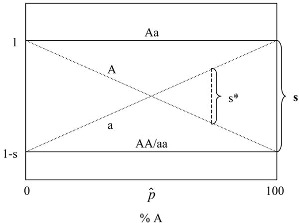When the two homozygotes have the same fitness, occurs at p = .5, where the two alleles have the same frequencies within the population (p refers to the percentage of one of the alleles, A, in the population). Since selection requires there to be variation in fitness, from the genic perspective no selection occurs at equilibrium. In contrast, when one looks at HeS from the genotypic perspective, the fitnesses of the genotypes vary at all allelic frequencies (even when the population is at equilibrium). Thus, the difference in fitness between the genotypes remains constant, and selection can be said to be equally strong regardless of allelic frequency (see fig. 1).Footnote ³ In short, the genotypic model asserts that there is selection (variation in fitness) even at equilibrium; the genic account denies this.

Figure 1. 

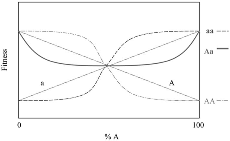
In figure 1, the intensity of selection is represented by the selection coefficients s and s*; A and a are the two alleles. The genotypic selection coefficient, s, is the difference in fitness between the genotypes and is frequency independent—it does not vary with the percentage of allele A in the population. In contrast, the genic selection coefficient, s*, is a weighted average of the genotypic fitnesses and is frequency dependent.Footnote ⁴ Significantly, while the value of s* at a given time can be derived from the value of s and the allelic frequencies that obtain at that time, one cannot derive the value of s from the value of s* and the allelic frequencies at a time. In fact, there are many possible genotypic fitness functions from which the same genic function could be derived (Denniston and Crow Reference Denniston and Crow1990). This is not merely a fact about the mathematical relationship between the models but indicates that a genic fitness function can be compatible with a wide range of biological interpretations. For example, Takahata and Nei (Reference Takahata and Nei1990) discuss an allelic fitness function that could potentially be the result of HeS but might alternatively result from a model in which the genotypic fitnesses are frequency dependent (fig. 2). Figures 1 and 2 show quite clearly that the genic model is less informative (logically weaker) than the genotypic one.

Figure 2. 

Sober and Lewontin argue that genic selectionism fails because the genic model misrepresents the causal processes occurring in the case of HeS. On their account, there is selection for entity X only if having X is beneficial in all causally relevant contexts. Since, with HeS, only the fitnesses of the heterozygote genotypes—but not those of the alleles—are beneficial across contexts, selection acts only on the genotypes.

Not everyone agrees that HeS presents a problem for genic selectionism. Sterelny and Kitcher (Reference Sterelny and Kitcher1988) argue that one can gain a full understanding of HeS at the level of the gene. They claim that Sober and Lewontin's definition of selection-for rules out the possibility of there being context-dependent selection. Yet, many clear cases of selection are context dependent, and HeS is just one more example. Sterelny and Kitcher suggest that when looking at an allele in a diploid genotype, one relevant context is the other allele in the genotype, which determines whether it has the fitness of the heterozygote or of the homozygotes. HeS therefore does not differ from other, undisputed, cases of context-dependent selection.

HeS is only one case that has been discussed in the debate over units of selection.Footnote ⁵ What the articles by these two pairs of authors show is that when participants in the debate have disagreed about HeS, the dispute was not about the predictive accuracy of the different selection models but about whether they provide equally good explanations. As Sober and Lewontin explain: “The defects of genic selectionism concern its distortion of causal processes, not whether its models allow one to predict future states of the population” (Reference Sober and Lewontin1982, 163).

What distinguishes the article by B&N from earlier criticisms of genic selectionism is its claim that genic and genotypic models for HeS are different not just in their explanatory power but also in what they predict. More specifically, they contend that the models make distinct probabilistic predictions about whether a population will remain at equilibrium. Furthermore, they claim, the predictions made using the genotypic selection model are the correct ones. If the genotypic model is empirically adequate while the genic model is not, there can be little question as to which should be adopted, and the debate would be resolved. B&N's argument, therefore, requires scrutiny.

3. The Argument

B&N claim that the genic and genotypic models for HeS disagree about whether selection or drift is the dominant process in a population and infer from this disagreement that the models make conflicting predictions. My primary criticism of B&N's argument will be that the two models do not disagree about whether selection or drift is the dominant process and that their argument is therefore unsound.

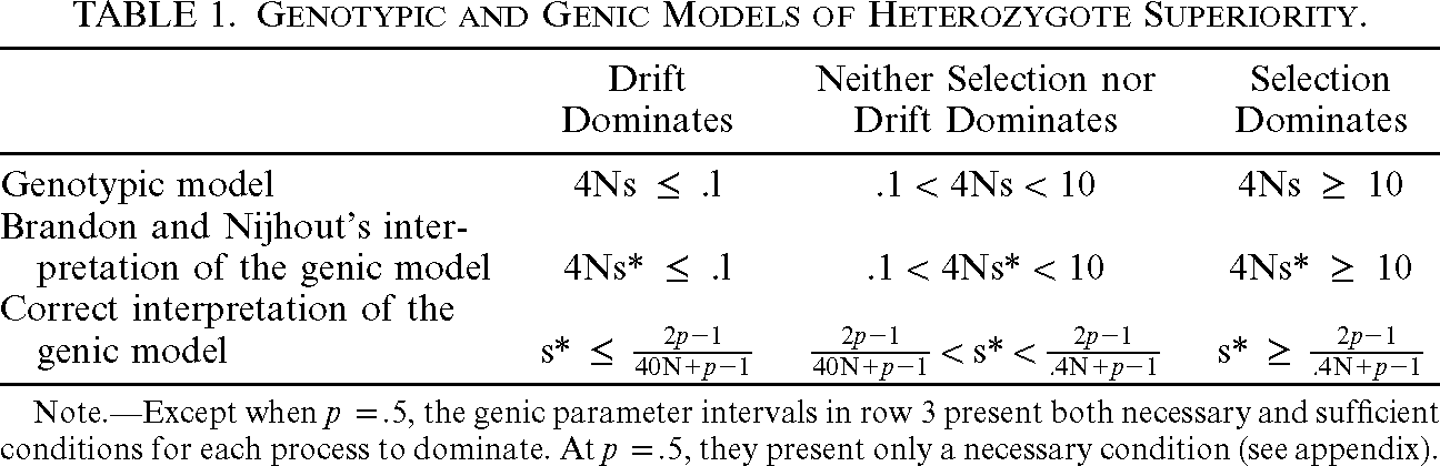
For both the genotypic and the genic models of HeS, B&N specify the parameter intervals for which each process dominates, as can be seen in the first two rows of table 1. Let's begin with the first row of the table. B&N follow geneticists in determining whether selection or drift dominates (or that neither does) by considering the product of N (the effective population size) and s (the genotypic selection coefficient). In sections 4 and 5, I will say more about how B&N choose the values in the first row, but for now I will treat them as unproblematic. The real difficulty with B&N's argument is with how they determine whether selection or drift dominates using the genic selection coefficient s*. The parameter intervals they use are given in the second row of the table. I will argue that the second row is incompatible with the first; if you understand “selection dominates drift” and “drift dominates selection” in the way described in row 1, you should not accept the values given in row 2. Instead, you should accept the parameter intervals in row 3 since they are a mathematical consequence of those in the first row. As the authors claim that the models diverge in their predictions is based on the incorrect values in the second row, their argument is unsuccessful.

Table 1Genotypic and Genic Models of Heterozygote Superiority.

	Drift Dominates	Neither Selection nor Drift Dominates	Selection Dominates
Genotypic model	4Ns ≤ .l	.1 < 4Ns < 10	4Ns ≥ 10
Brandon and Nijhout's interpretation of the genic model	4Ns* ≤ .l	.1 < 4Ns* < 10	4Ns* ≥ 10
Correct interpretation of the genic model

Note Except when p =.5, the genic parameter intervals in row 3 present both necessary and sufficient conditions for each process to dominate. At p =.5, they present only a necessary condition (see appendix).

4. Modeling Selection versus Drift

B&N's method of determining whether selection or drift dominates in a population comes from Roughgarden (Reference Roughgarden1979). Roughgarden presents an equation for predicting equilibrium distributions given the size of a population (N) and the genotypic selection coefficients. In cases of HeS where the two homozygotes are equally fit, one can see a clear trend for the interaction between selection and drift. When comparing populations of equal size and with the same initial polymorphic allelic distributions, those with a higher genotypic selection coefficient s are more likely to be close to the equilibrium value (p = .5) after a fixed number of generations. When comparing similar populations of varying sizes, drift is less strong in larger populations, so selection can maintain a large population around even if s is relatively low. Consequently, large populations with high selection coefficients are more likely to be at equilibrium than smaller populations with lower selection coefficients.

Both selection and drift are probabilistic processes, so there is no outcome that deductively settles whether selection or drift was responsible for the observed distribution of alleles. For example, if we find a population where p = 1 and know the values of the genotypic (and hence the genic) selection coefficients, we do not know for sure that drift was stronger than selection since even for large selection coefficients, some populations will end up having one allele go to fixation (although this is rare). What we can say is that for some values of N and s, it is probable that we will get the polymorphic population structure predicted by selection alone, and for others, we expect to see the lack of diversity predicted by drift. Roughgarden gives 4Ns = 1 as a useful value for separating the cases in which each outcome is likely to occur. More specifically, Roughgarden claims: “If 4Ns ≪ 1, then most populations possess little genetic variation and we might say that drift has overpowered selection. If 4Ns ≫ 1, then many populations are polymorphic as would be predicted from the deterministic theory” (Reference Roughgarden1979, 78). When 4Ns is much greater than 1, drift is weak enough to be “safely ignored” (78).

In any genetically diverse population of finite size, there will be drift, and in any case where there are fitness differences, there will be selection. When one specifies parameter values for when selection or drift will be said to dominate in a population, one is not making an empirical prediction but classifying the population on the basis of which process will be more significant in leading to the predicted outcome. On the basis of the values of N and s, one can predict that a population has a certain probability of straying from equilibrium. When Roughgarden says, for example, that selection dominates when 4Ns ≫ 1, this is not an additional prediction but a way of classifying the predictions made by the model. To make this classification is to decide how probable it must be that a population will remain at equilibrium in order to say that selection is the dominant process. While there might be further questions about whether the value specified should be 4Ns (as opposed to, say, 5Ns), there is no need to address them here. What is important is that once one has made a prediction on the basis of values of N and s, how one affixes the labels “selection dominates” and “drift dominates” has no further predictive significance.

5. The Proper Parameter Intervals for s*

Roughgarden never specifies precise parameter intervals outside of which either selection or drift dominate, beyond specifying that neither will dominate when 4Ns is approximately equal to 1. B&N provide more precise intervals in order to have a way of quantitatively comparing the genotypic and genic models. The parameter intervals they choose are as follows: if 4Ns ≥ 10, selection dominates; if 4Ns ≤ .1, then drift dominates; when 0.1 < 4Ns < 10, then neither dominates. Since s is the genotypic selection coefficient, these are the parameter intervals that they associate with the genotypic model of selection.

Once the parameter intervals that define “domination” for the genotypic model have been specified, we still need to find the corresponding ones for the genic model. First, we must derive the genic selection coefficient s* from the genotypic one. B&N do so using the following equation:

This equation allows one to derive the difference in fitness between the two alleles, A and a, given the frequency, p, of A in the population and the genotypic selection coefficient s. Since the genic model uses the genic selection coefficient s* instead of s, B&N need to specify how to apply to s* the classifications they associate with the genotypic model. They assume that the value of 4Ns* should play exactly the same role as that of 4Ns in determining which process dominates. In other words, they require the genic model to say that selection dominates when 4Ns* ≥ 10, drift dominates when 4Ns* ≤ .1, and neither dominates when 0.1 < 4Ns* < 10 (see table 1, row 2). I will argue that these parameter intervals are incompatible with those they provide for the genotypic model (in the first row of the table) and will provide a classification for the genic model that is not only consistent with the classification they use for the genotypic model but is a deductive consequence of the genotypic classification.

In finding the genic classification for when selection or drift dominates that corresponds to that of the genotypic model, it is key that when we replace s with s*, we also must change the range of parameter values outside of which drift or selection dominates. B&N have already provided a way of deriving s* from s (with (c)). Using this equation, we can derive the new parameter values for the genic model (see appendix), as shown in the third row of table 1. Notice that the new values look very different from those presented by B&N. It is now the case that in order to use s* to determine whether selection or drift dominates, one must also give a specific value for p. This, however, should not be surprising. Since s*, unlike s, is frequency dependent (fig. 1), it is to be expected that in order to know whether selection or drift dominates in a population, one must also know the relevant value of p.

If one accepts B&N's genotypic classifications summarized in row 1 of table 1, but classifies the genic model using parameter intervals other than those presented in row 3 of the table, then differences between the two models regarding whether selection or drift dominates will not reflect predictive disagreements. This can be made clear with an analogy. Imagine I define “Sarah runs much faster than Mike” to mean that Sarah's speed is greater than Mike's by at least 1 kilometer per hour (kph). If, using my definition, someone informs me that Sarah does, in fact, run much faster than Mike, I can use this to make a prediction about how much quicker she will finish a race. Now imagine I am asked to define whether Sarah is much faster than Mike, but this time using miles per hour (mph). Once I have defined “much faster than” as a difference of at least 1 kph, I must also define it as .62 mph. If I were to give any other value than .62 mph, my definition of “much faster than” would be inconsistent with my initial one. Furthermore, if my definitions were inconsistent, then the fact that the two “models”—given by my two definitions—disagree regarding whether Sarah is much faster than Mike will not tell me whether they make different predictions for how much faster she will win a race. Similarly, unless we interpret the genic model so that it classifies cases where drift dominates selection, or vice versa, in the same way as the genotypic model does, the fact that the models “disagree” in their classifications will not imply that they make conflicting predictions. Just as I could not replace “1 kph” with “1 mph” in the analogy, one cannot simply replace s with s* in the definition of domination and assume that the fact that they have different values reveals a predictive disagreement.Footnote ⁶

B&N are mistaken in holding that the genotypic and the genic models disagree about whether selection dominates drift. Since the genotypic model entails the genic model, once one has adopted a genotypic definition of “domination,” one must use a definition for the genic model that agrees with the genotypic definition. If we adopt the classification in row 1 of table 1, we must also adopt that given in row 3; row 2, which shows B&N's classification, is not correct.

6. Genic Predictions at Equilibrium

B&N often focus on the equilibrium point (p =.5), where the difference between the models is most pronounced. Here, the genotypic model claims that there is selection (s > 0), while the genic model claims there is not (since s* = 0). If there were any way to make a prediction about how a population will behave just by looking at the relative forces of selection and drift, the predictions at this point would have to be different. As B&N put it, “At equilibrium, the genic selectionist must predict that drift will dominate the transition to the next generation (because 4Ns* = 0)” (Reference Brandon and Nijhout2006, 282). Even after we have rejected B&N's classification of the genic model, one might think that since the genic model claims there is no selection at equilibrium, it must make an empirically different prediction.

One thing to notice is that at equilibrium the correct formulation of the genic model will not be of use. When p = .5, the genic parameter intervals only provide the necessary conditions for each process to dominate (see appendix); drift dominates only if s* ≤ 0, selection dominates only if s* ≥ 0. Since these are not sufficient conditions, the genic model entails neither that selection dominates nor that drift does. Consequently, B&N's assertion that the genic model must incorrectly classify the population at equilibrium as one in which drift dominates is false. The genic model does not classify at all in this case.

One might construe the inability of the genic model to say which process dominates to lend credence to B&N's argument. This is not the case. First of all, as soon as a population diverges even infinitesimally from equilibrium, the two models make equivalent classifications and predictions. More important, cases for which the genotypic model makes a prediction, while the genic model fails to do so, do not provide empirical evidence favoring one model over the other. As we have seen, the fact that the genotypic model is more informative has been known for decades. What B&N require is a set of observations for which the genotypic and genic models make different predictions.

7. How Should the Genic Selectionist Classify the Genic Model?

Given their classification of when selection or drift dominates in the genotypic model, B&N must classify the genic model in the way I suggest. I have not presented an argument for why the genic selectionist should accept this system of classification, beyond the fact that it is consistent with that of the genotypic model. Does this omission suggest that it is an open question whether the genic selectionist should accept my classification or that given by B&N? If so, one might wonder in what sense I have shown B&N's argument to be unsuccessful. My response is that while the genic selectionist could adopt genic classifications that are inconsistent with the genotypic ones, it is difficult to see why she would. If B&N had provided the only possible genic classifications, their assertion that genic selectionists are committed to their classifications would be plausible. Once one sees that there is an alternative set of classifications that is consistent with the genotypic ones, the claim that the genic selectionist must accept B&N's classifications loses all plausibility. B&N offer no defense of their genic classifications; the only apparent motivation for using them is their superficial similarity to those of the genotypic models.

8. Conclusion

At the beginning of their article, B&N claim that a major reason that the units-of-selection debate continues to attract attention is that “the refutations have primarily relied on philosophically contentious views on scientific explanation and causation—views their opponents have not been willing to accept” (Reference Brandon and Nijhout2006, 278). The implication is that the best way to resolve the debate would be through the empirical refutation of genic selectionism they claim to provide. No doubt, a successful argument that the genic and genotypic models make conflicting predictions would fundamentally change the nature of the debate. Yet, it would be wrong to suggest that lacking such an argument, we remain stuck in a philosophical stalemate. The genic and genotypic models might not make conflicting predictions, but it remains the case that the genotypic model is more informative. Of course, the genic selectionist can claim that the information missed by the genic model is explanatorily irrelevant, but this claim has become increasingly less plausible. The case described by Takahata and Nei (fig. 2), for example, reveals that genic models are unable to differentiate between radically different biological interpretations. Cases like this, which prima facie speak against the thesis that genic models provide the best framework for understanding selection, do not reveal a predictive difference between the higher- and the lower-level models. They do, however, lend credence to one of the earliest criticisms of genic selectionism—that much is missed at the level of the gene.