2.1. GNSS SF pseudorange measurement model

GNSS signals consist of electromagnetic waves that propagate at the speed of light and, from which, it is possible to determine the position of any point on or above the Earth’s surface (Groves, Reference Groves2013; Teunissen and Montenbruck, Reference Teunissen and Montenbruck2017). The range ${r_{as}}$ between satellite $s$ and receiver antenna $a$ is ideally obtained by measuring the propagation time of the GNSS signal, from its transmission by the satellite to its acquisition by the receiver, multiplied by the speed of light $c$ . As the receiver and satellite clocks are not synchronised with the official GNSS timescale, the measurements taken do not consist purely and simply of distances, being alternatively called pseudoranges. The raw (subscript $R$ ) pseudorange $\rho _{a,R}^{s,l}$ from satellite $s$ to user antenna $a$ for signal $l$ can be modeled as (Groves, Reference Groves2013; Hu et al., Reference Hu, Neupane and Farrell2022)

(1) \begin{align} \rho _{a,R}^{s,l} = {r_{as}} + \left( {\delta t_{sa}^a - \delta t_{st}^s} \right)c + \delta \rho _E^s + \delta \rho _{I,a}^{s,l} + \delta \rho _{T,a}^s + \delta \rho _{M,a}^{s,l} + \left( {{b^{a,l}} + {b^{s,l}}} \right)c + \delta w_{\rho, a}^{s,l}, \end{align}

where $\delta t_{sa}^a$ is the receiver clock error, $\delta t_{st}^s$ is the satellite clock error, $\delta \rho _E^s$ is the ephemeris/orbit error, $\delta \rho _{I,a}^{s,l}$ is the ionospheric error, $\delta \rho _{T,a}^s$ is the tropospheric error, $\delta \rho _{M,a}^{s,l}$ is the multipath error, ${b^{a,l}}$ and ${b^{s,l}}$ represent the code bias at the receiver and satellite hardwares, respectively, and $\delta w_{\rho, a}^{s,l}$ is the code tracking noise.

In the context of SF RT-SPP, estimates (symbol  ) for some of the CMEs displayed in Equation (1), namely, the orbit, ionospheric, satellite clock and hardware bias errors, can be computed and applied (see Section 2.2) to the raw pseudorange measurements, to obtain corrected (subscript $C$ ) observables:

(2) \begin{align} \rho _{a,C}^{s,l} = \rho _{a,R}^{s,l} + \delta \hat t_{st}^sc - \delta \hat \rho _E^s - \delta \hat \rho _{I,a}^{s,l} - \delta \hat \rho _{T,a}^{s,l} - {\hat b^{s,l}}c. \end{align}

Usually, for solving problems related to GNSS navigation, nonlinear estimators, such as the Iterated Weighted Least Squares (IWLS) or the Extended Kalman Filter (EKF), are used to calculate the position (and clock error) of the receiver (Farrell, Reference Farrell2008; Groves, Reference Groves2013; Grewal et al., Reference Grewal, Andrews and Bartone2013; Teunissen and Montenbruck, Reference Teunissen and Montenbruck2017). For the particular case of IWLS, the states generally comprise the Earth-Centred-Earth-Fixed (ECEF) Cartesian position of the receiver antenna, ${\bf{\hat r}}_{ea}^e$ , and the receiver range-domain clock error, $\delta \hat \rho _c^a = \delta \hat t_{sa}^ac$ , which are iterated (until a minimum threshold is reached that serves as a solution), as

(3) \begin{align} \left( {\matrix{ {{\bf{\hat r}}_{ea}^{e + }} \hfill \cr {\delta \hat \rho _c^{a + }} \hfill \cr } } \right) = \left( {\matrix{ {{\bf{\hat r}}_{ea}^{e - }} \hfill \cr {\delta \hat \rho _c^{a - }} \hfill \cr } } \right) + {[{({{\bf{H}}_W})^{\rm T}}{({\bf{C}}_\rho ^{ - 1})^{\rm T}}\left( {{{\bf{H}}_W}} \right)]^{ - 1}}{({{\bf{H}}_W})^{\rm T}}\left( {{\bf{C}}_\rho ^{ - 1}} \right)\left( {\matrix{ {\rho _{a,C}^{1,l} - \hat \rho _{a,C}^{1,l}} \hfill \cr {\rho _{a,C}^{2,l} - \hat \rho _{a,C}^{2,l}} \hfill \cr \ \ \ \ \ \ \vdots \hfill \cr {\rho _{a,C}^{m,l} - \hat \rho _{a,C}^{m,l}} \hfill \cr } } \right) \end{align}

where superscripts + and – denote estimates after and before each iteration, respectively, and $m$ is the number of visible satellites.

The pseudorange estimates employed in Equation (3) are computed as (Groves, Reference Groves2013)

(4) \begin{align} \hat \rho _{a,C}^{s,l} = \sqrt {\left[ {{\bf{C}}_e^I\left( {\hat t_{st}^s} \right){\bf{\hat r}}_{es}^e\left( {\hat t_{st}^s} \right) - {\bf{\hat r}}_{ea}^{e - }\left( {\hat t_{sa}^a} \right){]^{\rm T}}} \right[{\bf{C}}_e^I\left( {\hat t_{st}^s} \right){\bf{\hat r}}_{es}^e\left( {\hat t_{st}^s} \right) - {\bf{\hat r}}_{ea}^{e - }\left( {\hat t_{sa}^a} \right)]} + \delta \hat \rho _c^{a - }, \end{align}

where ${\hat t_{st}^s}$ is the time of signal transmission (from the satellite $s$ ), ${\hat t_{sa}^a}$ is the time of signal arrival (at the receiver antenna $a$ ), ${{\bf{\hat r}}_{es}^e}$ is the ECEF Cartesian position of satellite $s$ and ${\bf{C}}_e^I$ is the Sagnac compensation matrix according to which the ECEF frame is rotated during the GNSS signal propagation (Groves, Reference Groves2013).

The measurement matrix ${{\bf{H}}_W}$ , depicted in Equation (5), is computed as the Jacobian matrix of the measurement innovations w.r.t. the state innovations, i.e.

(5) \begin{align} {{\bf{H}}_W} = \left( {\matrix{ { - {\bf{u}}_{a1,x}^e}\ { - {\bf{u}}_{a1,y}^e}\ { - {\bf{u}}_{a1,z}^e}\ 1 \cr { - {\bf{u}}_{a2,x}^e}\ { - {\bf{u}}_{a2,y}^e}\ { - {\bf{u}}_{a2,z}^e}\ 1 \cr \ \ \ \ \vdots\ \ \ \ \ \ \ \ \ \vdots\ \ \ \ \ \ \vdots\ \ \ \ \vdots \cr { - {\bf{u}}_{am,x}^e}\ { - {\bf{u}}_{am,y}^e}\ { - {\bf{u}}_{am,z}^e}\ 1 \cr } } \right), \end{align}

where ${[ - {\bf{u}}_{am,x}^e{\rm{\;}} - {\bf{u}}_{am,y}^e{\rm{\;}} - {\bf{u}}_{am,z}^e]^T}$ is the ECEF-resolved unit line-of-sight vector between satellite $m$ and the receiver antenna $a$ .

The measurement noise covariance matrix ${{\bf{C}}_\rho }$ lastly, is given by

(6) \begin{align} {{\bf{C}}_\rho } = {\rm{diag}}\left[ {\matrix{ {\sigma _\rho ^2\left( {\theta _{nu}^{a1}} \right)\ \ \ \sigma _\rho ^2\left( {\theta _{nu}^{a2}} \right)\ \ \ \ldots \ \ \ \sigma _\rho ^2\left( {\theta _{nu}^{am}} \right)} \hfill \cr } } \right], \end{align}

where ${\sigma _\rho }$ is the pseudorange standard deviation, which is herein modelled as a function of the satellite $s$ elevation angle $\theta _{nu}^{as}$ .

When an EKF is employed instead of an IWLS, the receiver position and clock error are recursively (other than iteratively) updated (superscript +) based on a priori predictions (superscript −) of the latter, which are propagated in time based on the following dynamic evolution models:

(7)

(8)

(9)

where ${\bf{v}}_{ea}^e$ and $\dot \rho _c^a$ are the ECEF receiver antenna velocity and range rate-domain clock drift, respectively.

Unlike the IWLS (Equation (3)), the EKF updates the receiver position and clock error jointly with the receiver velocity and clock drift, which now becomes part of the state vector; and the measurement innovations are weighted by the so-called Kalman gain. In equations,

(10)

with

(11) \begin{align} {\bf{K}} = {{\bf{P}}^ - }{\bf{H}}_E^T{\left( {{{\bf{H}}_E}{{\bf{P}}^ - }{\bf{H}}_E^T + {{\bf{C}}_\rho }} \right)^{ - 1}}, \end{align}

(12) \begin{align} {{\bf{H}}_E} = \left( {\matrix{ { - {\bf{u}}_{a1,x}^e}\ { - {\bf{u}}_{a1,y}^e}\ { - {\bf{u}}_{a1,z}^e}\ 0\ 0\ 0\ 1\ 0 \cr { - {\bf{u}}_{a2,x}^e}\ { - {\bf{u}}_{a2,y}^e}\ { - {\bf{u}}_{a2,z}^e}\ 0\ 0\ 0\ 1\ 0 \cr \ \ \ \ \vdots\ \ \ \ \ \ \ \ \ \vdots\ \ \ \ \ \ \vdots\ \ \ \ \vdots\ \ \vdots\ \ \vdots\ \ \vdots\ \ \vdots \cr { - {\bf{u}}_{am,x}^e}\ { - {\bf{u}}_{am,y}^e}\ { - {\bf{u}}_{am,z}^e}\ 0\ 0\ 0\ 1\ 0 \cr } } \right) \end{align}

where ${\bf{P}}$ is the EKF error state covariance matrix. For additional details on the EKF deployment for GNSS position solutions, please refer to previous works (Farrell, Reference Farrell2008; Groves, Reference Groves2013; Grewal et al., Reference Grewal, Andrews and Bartone2013; Teunissen and Montenbruck, Reference Teunissen and Montenbruck2017).

2.2. RT-SPP correction models

SPP, either in its PP or RT variations, as well as other advanced GNSS positioning techniques, such as code-based DGNSS and RGNSS, aims at compensating for the CMEs introduced in Section 1, which correspond to the $\delta t_{st}^s$ , $\delta \rho _E^s$ , $\delta \rho _{I,a}^{s,l}$ , $\delta \rho _{T,a}^s$ and ${b^{s,l}}$ error terms defined in Equation (1). IGS, via its RTS, is the main organisation responsible for broadcasting free-of-cost RT products that allow users to correct for such CMEs (as in Equation (2)). The products are broadcast over the Internet using the Networked Transport of RTCM via Internet Protocol (NTRIP) using Radio Technical Commission for Maritime Services (RTCM) messages in State Space Representation (SSR) format. So far, the sole CME for which no RT-PPP products have been broadcast is the tropospheric error (corrections for the latter are foreseen only in stage 3 of IGS RTS deployment). Users interested in compensating for such error, therefore, still have to model them as additional states in their estimators (Askne and Nordius, Reference Askne and Nordius1987; Sapucci, 2001; Oliveira et al., Reference de Oliveira, Monico and Sapucci2017; Pereira et al., Reference Pereira, Machado and Marques2021) or resort to empirical models that take into account typical seasonal variations in atmospheric parameters, such as temperature, pressure and relative humidity as a function of location (Leandro et al., Reference Leandro, Santos and Langley2006; Böhm et al., Reference Böhm, Werl and Schuh2006; Böhm et al., Reference Böhm, Lagler, Schindelegger and Krásná2012; Landskron and Böhm, Reference Landskron and Böhm2017). For details on applicable tropospheric models and performance over Latin America, the interested reader is invited to refer to Oliveira et al. (Reference Oliveira, Ramos, Silva and de Lima2023).

The naming convention for the RT-PPP products was introduced by the IGS RTWG, so that ‘mount points’ have the pattern ‘TTTTXXAAAF’, where the type of flow (TTTT) can be: (a) SSRA, which is the SSR correction flow (conveying orbits, clocks, etc.), with orbits referring to the satellite Antenna Phase Centres (APCs); (b) SSRC, which is the SSR correction stream with orbits referring to the satellite antenna Centre of Mass (CoM); (c) DCBS, which is the SSR correction stream conveying Differential Code Biases (DCBs) only; (d) IONO, which conveys ionospheric correction; (e) TROP, which conveys tropospheric correction; and (f) BCEP, which is the navigation data stream containing the broadcast ephemeris. It is worth noting that SSRA and SSRC may also contain DCBs, ionospheric, tropospheric and phase bias corrections. Following the mount point pattern, XX is a two-digit solution identifier, AAA is a three-digit code for the AC and F is a one-digit format identifier (1 for IGS SSR messages) (BKG, 2022).

2.2.1. IGS SSR satellite orbit correction

The IGS SSR orbit correction message contains the parameters for orbit corrections $\delta {\bf{O}}$ in radial ( ${e_{{\rm{radial}}}}$ ), longitudinal ( ${e_{{\rm{along}}}}$ ) and transverse ( ${e_{{\rm{cross}}}}$ ) components. These orbit corrections are used to calculate a satellite position correction $\delta {\bf{r}}$ , to be combined with the ECEF Cartesian satellite position ${\bf{r}}_{es,B}^e$ calculated from the broadcast (subscript $B$ ) ephemeris. The corrected satellite position ${\bf{r}}_{es,C}^e$ is obtained as (IGS, 2020)

(13) \begin{align} {\bf{r}}_{es,C}^e = {\bf{r}}_{es,B}^e - \delta {\bf{r}}. \end{align}

The satellite position correction $\delta {\bf{r}}$ is calculated according to

(14) \begin{align} \delta {\bf{r}} = \left[ {{e_{{\rm{radial}}}}\ \ {e_{{\rm{along}}}}\ \ {e_{{\rm{cross}}}}} \right]\delta {\bf{O}}, \end{align}

with

\begin{align}\matrix{ {{e_{{\rm{along}}}} = {{{\bf{v}}_{es,B}^e} \over {\left| {{\bf{v}}_{es,B}^e} \right|}},} \hfill \cr {{e_{{\rm{cross}}}} = {{{\bf{r}}_{es,B}^e \times {\bf{v}}_{es,B}^e} \over {\left| {{\bf{r}}_{es,B}^e \times {\bf{v}}_{es,B}^e} \right|}},} \hfill \cr {{e_{{\rm{radial}}}} = {e_{{\rm{along}}}} \times {e_{{\rm{cross}}}},} \hfill \cr } \end{align}

where ${\bf{v}}_{e,B}^e$ is the ECEF satellite velocity computed from the broadcast ephemeris and $\delta {\bf{O}}$ is the complete correction vector for the orbit, which is calculated from the individual correction terms and their rates, as follows:

(15) \begin{align} \delta {\bf{O}} = \left[ {\matrix{ {\delta {{\bf{O}}_{{\rm{radial}}}}} \hfill \cr {\delta {{\bf{O}}_{{\rm{along}}}}} \hfill \cr {\delta {{\bf{O}}_{{\rm{cross}}}}} \hfill \cr } } \right] + \left[ {\matrix{ {\delta {{{\bf{\dot O}}}_{{\rm{radial}}}}} \hfill \cr {\delta {{{\bf{\dot O}}}_{{\rm{along}}}}} \hfill \cr {\delta {{{\bf{\dot O}}}_{{\rm{cross}}}}} \hfill \cr } } \right]\left( {t - {t_0}} \right). \end{align}

In Equation (15), $t$ is the current computation time and ${t_0}$ is the GNSS reference time obtained from the SSR orbit correction message, which is broadcast to users typically every 5 s.

For applying the IGS SSR satellite orbit correction, there are two options: (a) either the user (with access to the GNSS navigation message) uses the corrected satellite position from Equation (13) for computing the estimated pseudorange and satellite-to-receiver unit vector (as in Equations (4) and (5)), in which case no correction for $\delta \rho _E^s$ is needed in Equation (2); or (b) the latter is computed and applied to Equation (2) as (Rahman et al., Reference Rahman, Silva, Jiang and Farrell2022)

(16) \begin{align} \delta \hat \rho _E^s = {{{\bf{\hat r}}_{ea}^e - {\bf{\hat r}}_{es,C}^e} \over {\left| {{\bf{\hat r}}_{ea}^e - {\bf{\hat r}}\,_{es,C}^e} \right|}}{\rm{\;}}.{\rm{\;}}\left( {{\bf{\hat r}}_{es,B}^e - {\bf{\hat r}}_{es,C}^e} \right). \end{align}

2.2.2. IGS SSR satellite clock correction

The IGS SSR clock correction message contains the parameters to compute the clock correction $\delta C$ to be applied to the satellite clock error calculated according to the broadcast ephemeris. The precise satellite clock error to be used in Equation (2) can be obtained as

(17) \begin{align} \delta \hat t_{st}^s = \delta t_{st,B}^s + {{\delta C} \over c}, \end{align}

where $\delta t_{t,B}^s$ is the satellite clock error computed according to the GNSS Interface Control Document (ICD) from the broadcast clock parameters, identified by the GNSS Issue of Data (IOD) of the corresponding SSR clock correction message. The clock correction is formed by the following third-order polynomial:

(18) \begin{align} \delta C = {C_0} + {C_1}\left( {t - {t_0}} \right) + {C_2}{(t - {t_0})^2}, \end{align}

where ${C_i}$ , i = $\left\{ {0,1,2} \right\}$ are the coefficients from the SSR clock correction message, which are broadcast to users typically every 5 s via NTRIP.

2.2.3. IGS SSR satellite hardware bias correction

Hardware delays are caused by the difference between the paths taken by the carriers in the hardware of the GNSS equipment front-ends (Teunissen and Montenbruck, Reference Teunissen and Montenbruck2017). These delays are relatively stable over time, and affect code and phase observables differently, as a function of the transmission frequencies (e.g. L1 and L2 for GPS). IGS has standardised the nomenclature of satellite hardware delays in terms of Observable-specific Signal Biases (OSBs) (Schaer, Reference Schaer2016), which are defined w.r.t. the ionosphere-free combination of signals that is used by each GNSS as a reference to calculate its clock solution ( $P\left( Y \right)$ signals at $L1$ and $L2$ in the case of GPS). For SF users of the Precise Positioning Service (PSS) of GNSS, the magnitude of this delay is determined during the satellite calibration process before launch and is known as the Timing Group Delay (TGD), whose values form part of the navigation messages broadcast by each satellite (Marques, 2012). For users of the Standard Positioning Service (SPS) of GNSS, in turn, the observables must compensate for an additional hardware delay that is only transmitted in the newer GNSS navigation messages (Groves, Reference Groves2013) and/or shall be obtained directly from RT-PPP services, such as IGS RTS. Users of the GPS SPS, for instance, employing the traditional $L1$ Coarse Acquisition (C/A) code (which is the focus of this work), should correct for ${b^{l,s}}$ in Equation (2) by forming the following DCB:

(19) \begin{align} {\hat b^{s,C/A}} = {{\left( {OS{B_{P1}} - OS{B_{C/A}}} \right)} \over c}, \end{align}

where $OS{B_l}$ , $l$ $ \in$ $P1$ , C/A is the range-domain satellite OSBs suffered by signal $l$ w.r.t. the $P1$ / $P2$ linear combination. These OSBs are broadcast by IGS RTS typically every 30 s in SSR format.

2.2.4. IGS SSR ionosphere correction

The IGS SSR ionospheric corrections consist of a GIM in the form of VTEC information, with a temporal resolution of 20 min, which is combined by the Polytechnic University of Catalonia (UPC) from individual solutions provided by several RT ionospheric ACs. The VTEC information is defined for TEC layers of infinitesimal thickness and is encoded using spherical harmonics, in Total Electron Content Units (1 TECU = 1016 electrons/m ${^2}$ ), as follows (IGS, 2020):

(20) \begin{align} VTEC\left( {{L_{pp}},{\lambda _{pp}}} \right) = \mathop \sum \limits_{n = 0}^N \mathop \sum \limits_{m = 0}^{min\left( {n,M} \right)} \left[ {{C_{nm}}{\rm{cos}}\left( {m{\lambda _s}} \right) + {S_{nm}}{\rm{sin}}\left( {m{\lambda _s}} \right)} \right]{P_{nm}}{\rm{sin}}{L_{pp}}, \end{align}

where $N$ and $M$ are the degree and order of the spherical expansion, respectively, $n,m$ are indices, ${C_{nm}}$ and ${S_{nm}}$ are the cosine and sine coefficients for the layers, also respectively (all broadcast, in SSR format, typically every 15 s), ${L_{pp}}$ and ${\lambda _{pp}}$ are the geocentric latitude and longitude of the Ionospheric Piercing Point (IPP) for the layer, respectively, ${\lambda _s}$ is the mean sun-fixed and phase-shifted longitude of the IPP for the layer (modulo 2 $\pi$ ), and ${P_{nm}}$ is the fully normalised associated Legendre function.

The latitude ${L_{pp}}$ and longitude ${\lambda _{pp}}$ in Equation (20) refer to the IPP at the altitude of the ionospheric layer, which is defined as the intersection of a straight line from the position of the receiver to the satellite and a sphere with the altitude of the ionospheric layer above the spherical Earth model (IGS, 2020). The IPP latitude ${L_{pp}}$ , in particular, can be calculated, in radians, as

(21) \begin{align} {L_{pp}} = {\rm{arcsin}}\left( {{\rm{sin}}\ {L_a}{\rm{cos}}{\psi _{pp}} + {\rm{cos}}\ {L_a}{\rm{sin}}{\psi _{pp}}{\rm{cos}}\ A} \right), \end{align}

where ${L_a}$ and ${\lambda _a}$ are the geocentric latitude and longitude of the receiver, respectively, $A$ is the azimuth of the satellite w.r.t. the receiver, on the spherical Earth model, and ${\psi _{pp}}$ is the central angle between the position of the receiver and the projection of the IPP on the spherical surface of the Earth, which is calculated, in radians, as

(22) \begin{align} {\psi _{pp}} = {\pi \over 2} - E - {\rm{arcsin}}\left( {{{{R_e} + {h_r}} \over {{R_e} + {h_I}}}{\rm{cos}}\ E} \right), \end{align}

where $E$ is the elevation angle of the satellite w.r.t. receiver on the spherical Earth model, ${R_e}$ is the Earth’s spherical radius of 6370 km, and ${h_a}$ and ${h_I}$ are the receiver and ionospheric layer altitudes above the spherical Earth model.

Provided that the following conditions are met:

\begin{align}{L_a} \ge {0^ \circ }\ \ \ {\rm{and\ \ \ \;tan}}{\psi _{pp}}{\rm{cos}}\ A \gt tan\left( {\pi /2 - {L_a}} \right) \end{align}

or

\begin{align}{{L_a}\lt {{0^\circ }\ \ \ {\rm{and}}\ \ \ \ - {\rm{tan}}{\psi _{pp}}{\rm{cos}}\ A} \gt tan\left( {\pi /2 + {L_a}} \right),} \end{align}

the IPP longitude can be calculated, in radians, according to

(23) \begin{align} {\lambda _{pp}} = {\lambda _a} + \pi - {\rm{arcsin}}\left( {{{{\rm{sin}}{\psi _{pp}}{\rm{sin}}\ A} \over {{\rm{cos}}\ {L_{pp}}}}} \right). \end{align}

In all other cases, the IPP longitude is calculated, in radians, as

(24) \begin{align} {\lambda _{pp}} = {\lambda _a} + {\rm{arcsin}}\left( {{{{\rm{sin}}{\psi _{pp}}\ {\rm{sin}}\ A} \over {{\rm{cos}}\ {L_{pp}}}}} \right). \end{align}

The IPP longitude, shifted by 2 h to the maximum TEC (approximate 14:00 local time), lastly, is calculated as

(25) \begin{align} {\lambda _s} = {\rm{mod}}\left[ {\left( {{\lambda _{pp}} + {{\left( {t - 50400} \right)\pi } \over {43200}}} \right),2\pi } \right], \end{align}

where the function mod $\left( { \cdot, \cdot } \right)$ returns the remainder of the division of the first term by the second.

After the VTEC values are calculated, they need to be mapped to STEC values based on the elevation of the satellites at the height of the corresponding ionospheric layer, transmitted in the SSR VTEC message. This can be implemented as follows:

(26) \begin{align} STEC = {{VTEC} \over {{\rm{sin}}\left( {E + {\psi _{pp}}} \right)}}. \end{align}

The range-domain ionospheric delay $\delta \rho _{I,a}^{s,l}$ , lastly, which is to be compensated for in Equation (2), can be estimated as

(27) \begin{align} \delta \hat \rho _{I,a}^{s,l} = {{40.3{\rm{\;}}STEC{\rm{\;}}{{10}^{16}}} \over {{f^2}}}, \end{align}

where $f$ is the GNSS carrier frequency.

2.2.5. MAGN ionosphere correction

To enable greater accuracy over South America, the Caribbean and the Antarctic Peninsula, FCAG-UNLP recently started to produce its own VTEC maps, based on a regional and denser network of GNSS CORSs (Mendoza et al., Reference Mendoza, Meza and Paz2019a, b). The ionospheric product, referred to by the authors by the acronym MAGN, is provided with an update period of 15 min in the IONosphere EXchange (IONEX) format regularly used by IGS to convey its final products (Schaer et al., Reference Schaer, Gurtner and Feltens1998).

MAGN is directly provided in terms of estimated $VTE{C_{j,k}}$ values on an equidistant grid with 0.5 degrees of resolution, for geocentric latitude ${L_j}$ and longitude ${\lambda _k}$ of the IPP. Application of the single-layer, spherical Earth model, however, requires interpolation for the actual IPP position location ( ${L_{pp}},{\lambda _{pp}}$ ). As suggested by Teunissen and Montenbruck (Reference Teunissen and Montenbruck2017), a suitable interpolation technique is the bilinear one, according to which the VTEC value at the IPP coordinates is computed as

(28) \begin{align} \eqalign { {VTEC\left( {{L_{pp}},{\lambda _{pp}}} \right) = \left( {1 - p} \right)\left( {1 - q} \right)VTE{C_{j,k}} + \left( p \right)\left( {1 - q} \right)VTE{C_{j + 1,k}}} \cr + \left( {1 - p} \right)\left( q \right)VTE{C_{j,k + 1}} + \left( p \right)\left( q \right)VTE{C_{j + 1,k + 1}},} \end{align}

where

(29) \begin{align} \matrix{ {p = {{{L_{pp}} - {L_j}} \over {{L_{j + 1}} - {L_j}}},} \hfill \cr {q = {{{\lambda _{pp}} - {\lambda _k}} \over {{\lambda _{k + 1}} - {\lambda _k}}},} \hfill \cr } \end{align}

is applied in the intervals ${L_j} \le {L_{pp}} \le {L_{j + 1}}$ and ${\lambda _k} \le {\lambda _{pp}} \le {\lambda _{k + 1}}$ , bounded by the surrounding grid points.

After VTEC is calculated, STEC and range-domain ionospheric delay computation follow the same procedure described in Equations (26) and (27). As the deployment of MAGN ionospheric corrections is very recent and its use is potentially important in the scope of CAV applications in South America, its performance assessment (via simulated RT processing) w.r.t. IGS SSR ionospheric products for RT-SPP, i.e. code-based SF RT-PPP, users stand out as the main investigation topic of this work. To the best of the authors’ knowledge, a comparison between these RT-PPP products has not been presented in the literature yet.

3.1. Dynamic test

The dynamic test consisted of collecting L1 C/A GPS observation data from a u-blox C102-F9R receiver and an ANN-MB-01 antenna attached to a car on July 21, 2023, in Lavras-MG, Brazil (Figure 1). The car was driven for a couple of minutes through the streets of a neighbourhood close to the Federal University of Lavras (UFLA), executing all types of motion that are typical for urban scenarios, such as curves, accelerations, decelerations, climbs, descents, stops, etc. (Figure 2). Along with the observation data, the BKG NTRIP Client (BNC) software was used to collect the SSR RT-PPP products from the IGS RTS, namely: (a) SSRA02IGS1, which is an IGS Kalman filter combined solution that conveys satellite orbit, clock and hardware bias corrections; and (b) IONO01IGS1, which is an RT VTEC GIM. The FCAG-UNLP RT VTEC products, i.e. MAGN, were collected directly from its File Transfer Protocol (FTP) server in the IONEX format (MAGGIA, 2022). To deploy the comparative DGPS strategy, as well as a reliable Ground-Truth (GT) solution, the GPS observation data and navigation message from the Lavras reference station (acronym MGLA), belonging to the Brazilian RBMC and distant to the car of approximately 1 km, were directly obtained from the Brazilian Institute of Geography and Statistics (IBGE) repository.

Figure 1.

Car used in the dynamic test.

Figure 2.

Ground-truth Three-Dimensional (3D) trajectory of the car in the dynamic test.

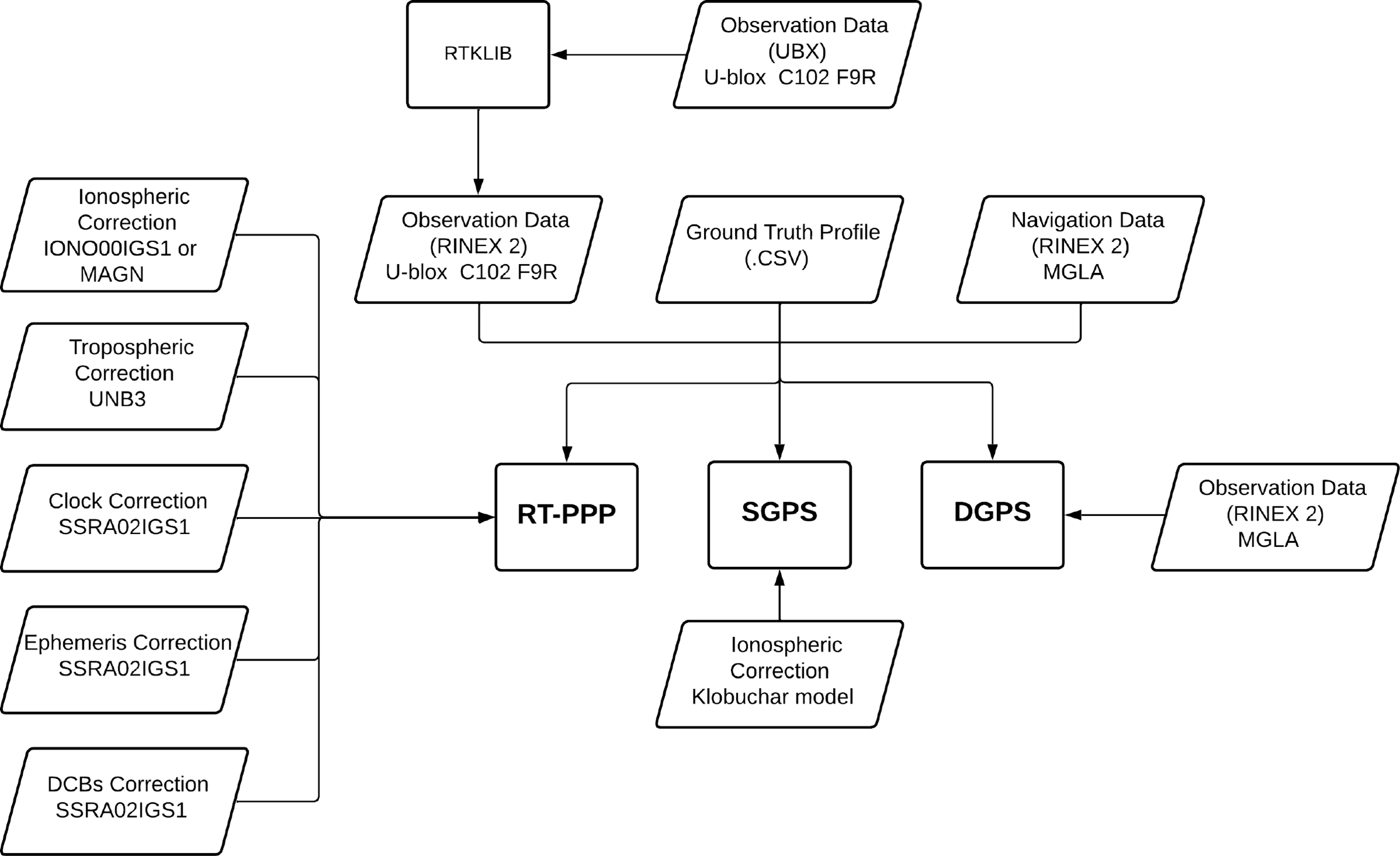
After the GPS data acquisition and conversion (from proprietary.UBX format to Receiver INdependent EXchange (RINEX) format version 2.11, via RTKLIB software (Takasu et al., Reference Takasu, Nubo and Yasuda2007)), the latter were processed offline and analysed using specialised MATLAB algorithms developed by the authors, which employed an EKF strategy to compute the position solutions (Teunissen and Montenbruck, Reference Teunissen and Montenbruck2017). The errors were calculated w.r.t. the GT profile, which was obtained by processing, also via an EKF, dual-frequency double-differenced pseudorange, and carrier-phase observables with integer ambiguity resolution from the u-blox C102-F9R module connected, via the Internet, to the MGLA reference station (Figure 1). The performance assessment of the tested strategies has only been performed when the integer ambiguities from the GT solution had already been reliably solved and fixed, which assured centimetre-level accuracy for the coordinate/position reference values. A mask angle of 15 degrees has been assumed for the whole test, in agreement with what has been recommended by Oliveira et al. (Reference Oliveira, Silva and de Lima2024) for SF GNSS users in Brazilian territory. Figure 3 contains a diagram with the input files of each of the investigated strategies for the dynamic test. Figure 4 and Tables 2– 4 summarise the main results in terms of Cumulative Distribution Functions (CDFs), mean values and Standard Deviations (STDs) of the horizontal, vertical and total position errors (best results are highlighted in bold fontFootnote ³ ).

Figure 3.

Diagram representing the dynamic test routines.

Figure 3. Long description

A diagram representing the dynamic test routines for satellite systems. The diagram includes various data sources and correction methods used in satellite positioning. Observation Data from U-blox C102 F9R is processed through RTKLIB and converted into RINEX 2 format. This data is then used in RT-PPP, SGPS, and DGPS systems. Ionospheric Correction data from ION001IGS1 or MAGN, Tropospheric Correction from UNB3, Clock Correction from SSRA02IGS1, Ephemeris Correction from SSRA02IGS1, and DCBs Correction from SSRA02IGS1 are applied to the RT-PPP system. Ground Truth Profile in CSV format and Navigation Data in RINEX 2 format from MGLA are also used. SGPS uses the Klobuchar model for ionospheric correction.

Figure 4.

Cumulative distribution of the position errors in the dynamic test.

Table 2.

Horizontal position error statistics for the dynamic test.

Table 3.

Vertical position error statistics for the dynamic test.

Table 4.

Total position error statistics for the dynamic test.

As can be seen, with respect to the lane-level position error requirement defined by Williams and Barth (Reference Williams and Barth2020) for CAV applications, namely, the provision of horizontal position solutions better than 1.0 m, at 95% probability, none of the investigated strategies were able to comply with the latter, whereas the DGPS strategy was the one that approached the most (62% probability). Regarding the more relaxed constraint established by the SAE J2945 standard, aimed at V2V communication applications, namely, the provision of horizontal and vertical position errors smaller than 1.5 and 3.0 m, respectively, at 68% probability, one verifies that: (a) in terms of horizontal position, DGPS was the best-performing method (80% probability), and only the latter and MAGN RT-SPP were able to comply with the aforementioned standard requirement; and (b) in terms of vertical position, all strategies were able to comply with SAE J2945 standard.

In terms of mean errors, the strategies that provided the best results, in decreasing order, were as follows: (a) for the horizontal channel – DGPS, MAGN RT-SPP, IGS RT-SPP and SGPS; (b) for the vertical channel – DGPS, SGPS, IGS RT-SPP and MAGN RT-SPP; and (c) for the total channel – DGPS, IGS RT-SPP, MAGN RT-SPP and SGPS. Specifically, in the horizontal channel, MAGN RT-SPP yielded a mean error of 1.18 m compared with 1.56 m for IGS RT-SPP, representing an absolute error reduction of 0.38 m (a relative improvement of 24.4%). These outcomes are in agreement with the recent verifications made by Silva et al. (Reference Silva, Hu and Farrell2023), who demonstrated, for similar dynamic conditions and RT-PPP products, the superior performance of MAGN w.r.t. IGS RTS VTEC for the horizontal channel, to the detriment of the vertical channel. These results, however, contradict the verifications of Pereira et al. (Reference Pereira, Machado and Marques2021), wherein MAGN performance was shown to be better than that of IGS PP VTEC in the vertical channel (consequently, MAGN should also be better than IGS RTS VTEC in this channel, as the latter is supposed to be worse than its PP counterpart).

Results from the IGS RT-SPP strategy, in particular, proved to be in agreement with previous results from de Bakker and Tiberius (Reference de Bakker and Tiberius2017), who obtained horizontal position accuracy better than 1.75 m at 77.7% of probability with their GPS-only SF RT-PPP approach. Comparatively, we obtained horizontal position errors better than 1.75 m at 69.5% of probability. It is important to stress, however, that in their work, Bakker and Tiberius employed a different tropospheric model, a 1-day predicted IGS VTEC product and carrier phase observations to smooth the pseudoranges (all of which contributed to improve the accuracy w.r.t. to our IGS RT- SPP strategy). In terms of vertical and total position accuracy, lastly, results from the IGS RT-SPP strategy also proved to agree with the verifications made by Hu et al. (Reference Hu, Neupane and Farrell2022), who achieved similar accuracies for their virtual network DGNSS approach (based on pseudoranges only and the same RT-PPP products from IGS RTS used in this work), namely, vertical and total position errors better than 3.0 m at 100% of probability.

Finally, it is worth mentioning that even though DGPS was the best performing strategy in the dynamic experiment, by delivering the smallest position errors mean values and the largest probabilities of the solutions to lie inside the pre-specified thresholds, it resulted in impaired STDs for the position errors (e.g. an absolute STD increase of 0.10 m or a relative increase of 18.5% in the horizontal channel when compared with MAGN RT-SPP). This is consistent with the fact that the SD process employed to process both the rover and reference station pseudoranges increases the noise in the resulting observables (Groves, Reference Groves2013).

3.2. Static tests

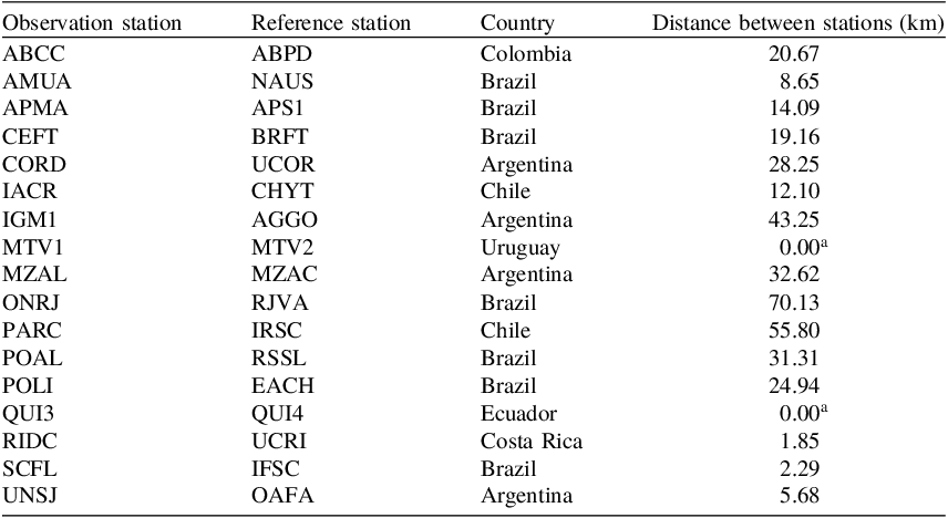
Even though the results from the dynamic test presented in Section 3.1 shed important light on the problem under investigation, namely, the comparative performances of IONO01IGS1 and MAGN ionospheric products for SF RT- SPP Latin American users, the latter are still limited in the sense they were based on GPS observation data: (a) with very short time duration (only a couple of minutes); and (b) that were confined to a specific location in Brazil. These limitations were also present in the recent works by Pereira et al. (Reference Pereira, Machado and Marques2021) and Silva et al. (Reference Silva, Hu and Farrell2023), and may mask the real achievable performance of the aforementioned RT-PPP products for Latin American users at different locations and different hours of the day. As the execution of a dynamic test that encompassed several hours would be somewhat cumbersome, we repeated the RT-PPP products comparison that is of interest for a series of long-duration tests (of approximately 12 h each, to cover the full orbiting period of the GPS constellation), using static CORSs belonging to the most relevant GNSS networks inside the coverage area of MAGN service, i.e. Latin America with extension to the Caribbean and Antarctica Peninsula. We chose the reference stations carefully so that each would have another reference station nearby (distanced at no more than 70 km, with an average of 21.81 km), which could be used for DGPS evaluation purposes (Table 5 and Figure 5).

Table 5.

Observation and reference stations employed in the static tests.

^a GNSS antennae are collocated.

Figure 5.

Observation stations employed in the static tests.

The static CORS observation data were acquired on June 22, 2023, in RINEX format, directly from the corresponding GNSS network repositories. Even though the CORSs were equipped with high-quality multi-constellation multi-frequency GNSS receiver equipment, only L1 C/A observation data from the GPS were considered, as this is the signal that Latin American users equipped with low-cost receivers (the focus of this work) are most likely to track in its CAV, V2V and/or V2X communication applications. The acquisition of the RT-PPP products under investigation followed the same procedure adopted in the dynamic test, namely, SSR RT-PPP products from the IGS RTS were acquired via BNC and MAGN VTEC directly from FCAG-UNLP FTP server, in IONEX format. After collection, we processed the data offline using specialised algorithms developed by the authors in the MATLAB framework, employing an EKF strategy to compute the position solutions. Whenever available, GPS Doppler shift observations in L1 frequency from the CORSs have also been used in the EKF for providing additional smoothing for the pseudoranges (Farrell, Reference Farrell2008; Groves, Reference Groves2013; Teunissen and Montenbruck, Reference Teunissen and Montenbruck2017).

The position solutions from the investigated strategies were compared against the actual positions of the CORSs, which are known to millimetre level, as they are frequently surveyed by the IBGE responsible personnel. Figures 6–8 present the probability of the strategies to provide horizontal position solutions with accuracies better than 0.5, 1.0 and 1.5 m, respectively (dotted lines highlight the probabilities of 68% and 95%). Table 6 summarises the latter in terms of mean and STD values for all observation stations (once again, the best results are highlighted in bold font).

Figure 6.

Probability of the horizontal position errors to be better than 0.5 m in the static tests.

Table 6.

Horizontal position error statistics for the static tests (mean $ \pm$ STD values).

As can be seen, if one seeks to meet the lane-level position accuracy constraints proposed by Williams and Barth (Reference Williams and Barth2020), none of the tested strategies would be able to provide us with satisfactory results. DGPS, for instance, which was the strategy that performed best, only provided horizontal position accuracy better than 1.0 m at 75% probability, on average (see Table 6 for details). Looking at Figure 6, we also see that DGPS positioning performance was highly (and inversely) correlated with the distance between the observation and reference stations, as expected. The MAGN RT- SPP strategy, in sequence, which was the second best-performing approach, delivered sub-meter-level accuracy at 63% of the time, also on average. Then, IGS RT- SPP followed, achieving sub-metre-level positioning at 38% probability, and lastly, SGPS, with only 26% (all the latter, on average).

Considering, alternatively, the compliance of the strategies with the V2V position requirements defined by the SAE J2945 standard, one sees that both DGPS and MAGN RT- SPP provided sufficiently accurate performance: DGPS delivered horizontal position solutions that were, on average, accurate to 1.5 m at 88% of time, while MAGN RT-SPP, at 86% of the time (see Table 6 for details). IGS RT-SPP and SGPS, in turn, failed to meet SAE J2945 standard requirements, by delivering, on average, horizontal position solutions better than 1.5 m at only 58% and 43% probability, respectively.

Figures 9–11, in sequence, depict the probability of the strategies to provide vertical position solutions below 1.0, 2.0 and 3.0 m, respectively (dotted lines highlight the probabilities of 68% and 95%). Table 7 summarises the latter in terms of mean and STD values for all observation stations (best results are highlighted in bold font). As verified at a glance, DGPS once again stands out as the best-performing strategy, delivering solutions that were, on average, accurate to 3.0 m at 95% of the time. IGS RT-SPP and MAGN RT-SPP, which were the second and third best-performing strategies (in agreement with the outcomes from the dynamic test), delivered performances very close to each other, namely, vertical position solutions better than 3.0 m at 79% and 75% of probability, respectively. SGPS, lastly, was the sole strategy that was not able to comply with SAE J2945 vertical position requirements, delivering 3.0 m-level position solutions at only 8% of the time.

Figure 7.

Probability of the horizontal position errors to be better than 1.0 m in the static tests.

Figure 8.

Probability of the horizontal position errors to be better than 1.5 m in the static tests.

Figure 8. Long description

A bar graph comparing the probability of horizontal position errors being better than 1.5 meters across different observation bases. The horizontal axis represents the observation bases, labeled as A B C C, A M U A, A P M A, C E F T, C O R D, I A C R, I G M 1, M T V 1, M Z A L, O N R J, P A R C, P O A L, P O L I, Q U I 3, R I D C, S C F L, and U N S J. The vertical axis represents the probability, ranging from 0 to 1. The graph includes four sets of bars for each observation base, representing different methods: S G P S, I G S R T S P P, M A G N R T S P P, and D G P S. Each set of bars is color-coded: blue for S G P S, orange for I G S R T S P P, yellow for M A G N R T S P P, and purple for D G P S. The graph shows that the probability varies significantly across different observation bases and methods. For instance, observation bases like C E F T, I A C R, and P O L I show high probabilities close to 1 for all methods, while others like A B C C and U N S J show lower probabilities, especially for the S G P S method.

Figure 9.

Probability of the vertical position errors to be better than 1.0 m in the static tests.

Figure 10.

Probability of the vertical position errors to be better than 2.0 m in the static tests.

Figure 10. Long description

A bar graph comparing the probability of vertical position errors being better than 2.0 meters across different observation bases. The horizontal axis represents the observation bases, labeled as A B C C, A M U A, A P M A, C E F T, C O R D, I A C R, I G M 1, M T V 1, M Z A L, O N R J, P A R C, P O A L, P O L I, Q U I 3, R I D C, S C F L, and U N S J. The vertical axis represents the probability, ranging from 0 to 1. The graph includes four sets of bars for each observation base, representing different methods: S G P S, I G S R T S P P, M A G N R T S P P, and D G P S. Each set of bars is color-coded: blue for S G P S, orange for I G S R T S P P, yellow for M A G N R T S P P, and purple for D G P S. The graph shows that the D G P S method consistently has the highest probability across all observation bases, followed by M A G N R T S P P, I G S R T S P P, and S G P S. Notable trends include the high probability for D G P S across all bases and the lower probability for S G P S in several bases.

Figure 11.

Probability of the vertical position errors to be better than 3.0 m in the static tests.

Table 7.

Vertical position error statistics for the static tests (mean $ \pm$ STD values).

Figures 12–14, lastly, present the probability of the strategies to provide position solutions with total errors below 1.0, 2.0 and 3.0 m, respectively, while Table 8 summarises the main results. As can be verified, DGPS was, as expected, the best-performing strategy, followed by MAGN RT- SPP, then IGS RT- SPP and, lastly, SGPS.

Figure 12.

Probability of the total position errors to be better than 1.0 m in the static tests.

Figure 13.

Probability of the total position errors to be better than 2.0 m in the static tests.

Figure 13. Long description

A bar graph compares the probability of total position errors being better than 2.0 meters across different observation bases using various GNSS signal processing methods. The horizontal axis represents the observation bases, labeled as A B C C, A M U A, A P M A, C E F T, C O R D, I A C R, I G M 1, M T V 1, M Z A L, O N R J, P A R C, P O A L, P O L I, Q U I 3, R I D C, S C F L, and U N S J. The vertical axis represents the probability, ranging from 0 to 1. The graph includes four sets of vertical bars for each observation base, representing different methods: S G P S in blue, I G S R T S P P in orange, M A G N R T S P P in yellow, and D G P S in purple. Each set of bars shows the probability values for the respective methods. Notable trends include higher probabilities for the D G P S method across most observation bases, with some variation in probabilities for the other methods.

Figure 14.

Probability of the total position errors to be better than 3.0 m in the static tests.

Table 8.

Total position error statistics for the static tests (mean $ \pm$ STD values).

Based on the preceding analysis, the following considerations are worthy of note: (a) in agreement with what we obtained in the dynamic test of Section 3.1, MAGN RT-SPP was shown to perform significantly better than its IGS RT-SPP counterpart for the horizontal channel. On average, MAGN RT-SPP was able to deliver horizontal position solutions at the same accuracy of those by IGS RT-SPP, 67% more in terms of probability (i.e. 26% vs 14% (86% improvement) for $P\left( { \le 0.5{\rm{\;m}}} \right)$ ; 63% vs 38% (66% improvement) for $P\left( { \le 1.0{\rm{\;m}}} \right)$ ; and 86% vs 58% (48% improvement) for $P\left( { \le 1.5{\rm{\;m}}} \right)$ ). Corroborating the latter verification, we observe from Figures 6–8 that MAGN RT-SPP outperformed IGS RT-SPP in 16, 15 and 15, respectively, out of the 17 static tests; (b) for the vertical channel, in turn, and also in agreement with the dynamic test and with previous results by Silva et al. (Reference Silva, Hu and Farrell2023), IGS RT- SPP performed better than MAGN RT-SPP. Considering all the 17 evaluated observation stations, IGS RT-SPP’s outcomes were more accurate than MAGN RT-SPP’s in 13, 11 and 11 of the latter, respectively, according to Figures 9–11. Despite this, the difference in performances proved not to be as noticeable as for the horizontal channel, since here, on average, IGS RT-SPP was better than its MAGN RT-SPP counterpart only by 13% in terms of percentile (i.e. 37% vs 30% (23% improvement) for $P\left( { \le 1.0{\rm{\;m}}} \right)$ ; 64% vs 58% (10% improvement) for $P\left( { \le 2.0{\rm{\;m}}} \right)$ ; and 79% vs 75% (5% improvement) for $P\left( { \le 3.0{\rm{\;m}}} \right)$ ); and (c) as a natural consequence of the preceding verifications, MAGN RT-SPP was proven to outperform IGS RT-SPP in terms of total position error, being able to deliver solutions at the same accuracy as those by IGS RT-SPP, 21% more in terms of probability (i.e. 17% vs 13% (31% improvement) for $P\left( { \le 1.0{\rm{\;m}}} \right)$ ; 52% vs 43% (21% improvement) for $P\left( { \le 2.0{\rm{\;m}}} \right)$ ; and 73% vs 66% (11% improvement) for $P\left( { \le 3.0{\rm{\;m}}} \right)$ ). In agreement with the latter verification, we observe from Figures 12–14 that MAGN RT-SPP outperformed IGS RT-SPP in 10, 10 and 8, respectively, out of the 17 static tests. Moreover, jointly with DGPS, MAGN RT-SPP was the sole RT- SPP strategy able to fully comply with SAE J2945 position requirements.

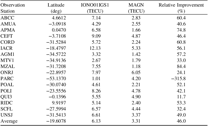
To more systematically evaluate the accuracies of the tested RT-PPP ionospheric products, namely, IONO01IGS1 from IGS RTS and MAGN from FCAG-UNLP, Figure 15 provides us with the VTEC estimates conveyed by each product right above (i.e. at the zenith of) all of the observation stations and for the whole duration of the static tests. For comparison purposes, the 11 days-delayed final combined VTEC product from IGS has also been included in Figure 15, to serve as a reliable reference GT. Table 9 summarises the results in terms of VTEC RMS errors for each observation station and tested RT-PPP ionospheric products. For ease of reference, Table 9 also provides the approximate latitude of each observation station as well as the relative improvement (in percentage) of MAGN VTEC predictions w.r.t. those from IONO01IGS1.

Figure 15.

VTEC, in TECU units, in the static tests.

Table 9.

VTEC RMS errors in the static tests.

As can be seen, all VTEC plots followed the expected ‘bell’ shape, centred at the time of day with the highest solar incidence, i.e. ionospheric ionisation (Teunissen and Montenbruck, Reference Teunissen and Montenbruck2017). Moreover, in almost all plots, the MAGN RT-PPP ionospheric VTEC products were the ones that more closely/nicely approached/fitted the corresponding GTs, which again corroborates the preceding verifications (improved position performance of MAGN RT-SPP w.r.t. IGS RT-SPP). Table 9, in particular, shows that MAGN conveyed ionospheric VTEC estimates that were, on average, 46% more accurate than those from IONO01IGS1 (i.e. 3.31 TECUs vs 6.13 TECUs, in terms of RMS errors). The only exception for the latter took place at the PARC observation station, wherein the IONO01IGS1 product predicted better the actual VTEC in comparison with MAGN (see Figure 15 and Table 9). Such an outcome is again in agreement with our previous positioning results. By looking at Figures 6–8, for instance, it is possible to observe that the very few occasions IGS RT-SPP performed better than MAGN RT-SPP (in terms of horizontal position errors) corresponded to the static tests conducted at the PARC observation station. The other two scarce occasions on which the latter behaviour repeated (for the horizontal channel) corresponded to QUI3 and SCFL observation stations, whose VTEC predictions from IONO01IGS1 and MAGN proved to be very close to each other (see Table 9 for details).

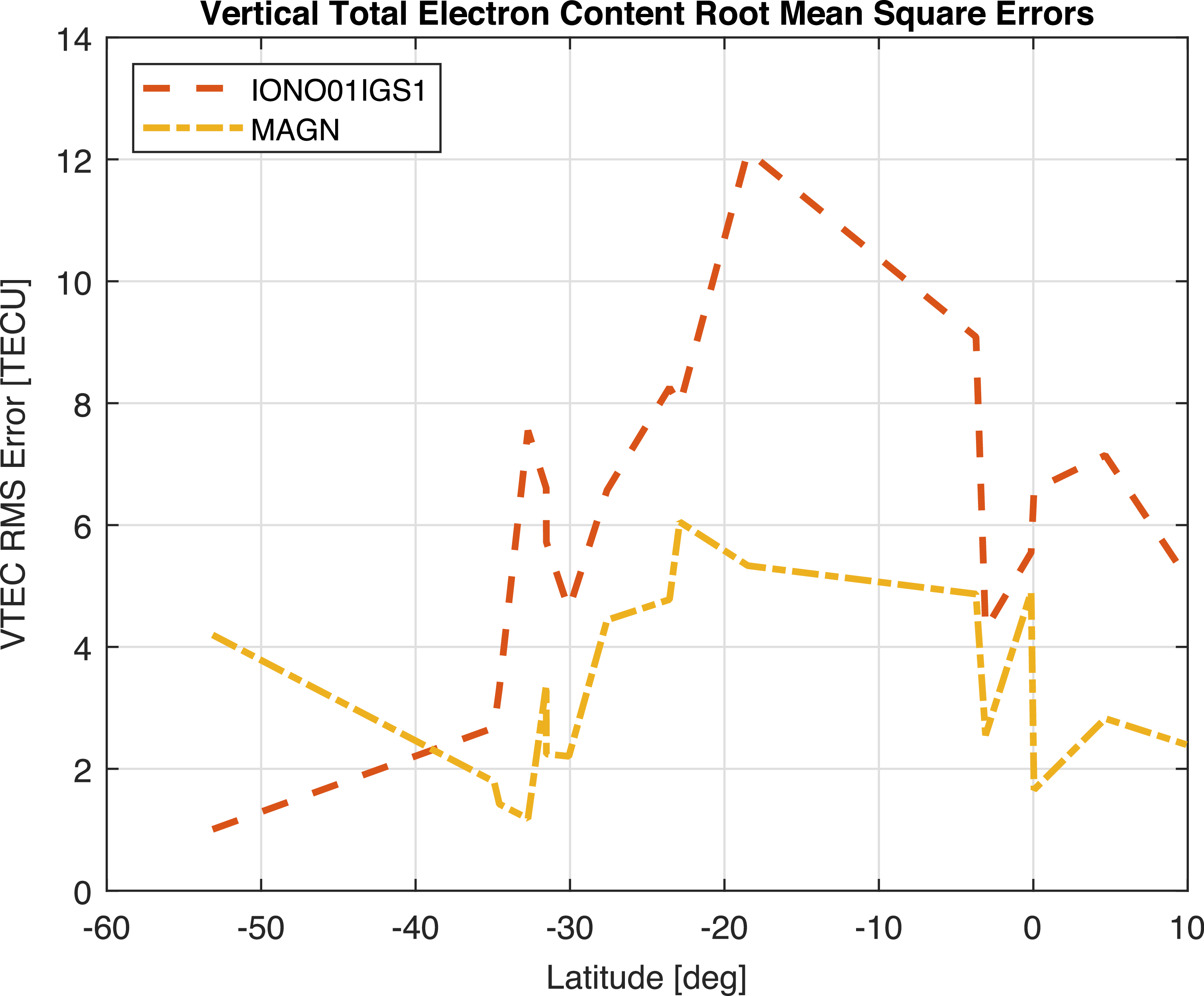
Aiming to assess the correlation between the observation station positions/locations and the accuracy of IONO01IGS1’s and MAGN’s VTEC estimates, Figure 16 plots the VTEC RMS errors of the latter as a function of the station latitudes. As can be seen, right below the Equator, the accuracy of both products deteriorated. Such verification is straightforward, as such tropical areas are more prone to solar incidence and, consequently, to ionospheric ionisation/scintillation (Marques et al., Reference Marques, Susi, Borio, Monico, Park and Wezka2024). The straightforward consequences of the latter are: (a) higher VTEC estimates for the stations situated around those places; and (b) potentially larger positioning errors. Both predictions are confirmed from Figure 15, as well as Figures 6–14, which evidence, for ABCC, AMUA, APMA, CEFT and QUI3 observations stations (all of which are situated in low latitude areas), higher levels of VTEC estimates and deteriorated positioning performances (regardless of the estimation method). The PARC observation station, in turn, which is situated at a very high latitude, displayed significantly smaller VTEC estimates, as well as superior positioning performance (again, regardless of the estimation method). Please see Figures 6, 12 and 15 for details.

Figure 16.

VTEC RMS errors, in TECU units, as a function of the observation station latitudes.

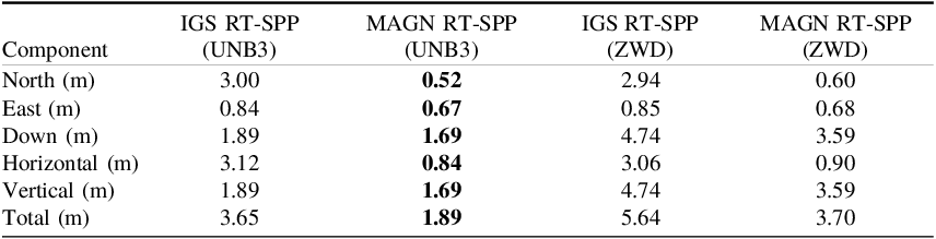
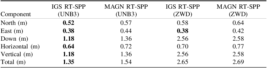
To supplement the analysis, Figures 17 and 18 plot the positioning errors of the observation stations MZAL and PARC, respectively, as a function of the GPS Time of Week (TOW). These stations are not only situated at different latitudes but also, according to Table 9, present the most significant (largest positive and negative) relative discrepancies in terms of ionospheric VTEC prediction performance. As can be seen, the outcomes once again corroborate the results depicted in Figures 6–14: the positioning performance at MZAL was favoured by MAGN, whereas at PARC, it was favoured by IONO01IGS1 (which proved to be an exception compared with the other observation stations).

Figure 17.

MZAL positioning performance as a function of GPS TOW.

Figure 18.

PARC positioning performance as a function of GPS TOW.

Figure 18. Long description

Panel A: A line graph depicts the North position error in meters over GPS Time of Week in seconds. The graph includes multiple data series represented by different colors. Panel B: A line graph depicts the Horizontal position error in meters over GPS Time of Week in seconds. The graph includes multiple data series represented by different colors. Panel C: A line graph depicts the East position error in meters over GPS Time of Week in seconds. The graph includes multiple data series represented by different colors. Panel D: A line graph depicts the Vertical position error in meters over GPS Time of Week in seconds. The graph includes multiple data series represented by different colors. Panel E: A line graph depicts the Down position error in meters over GPS Time of Week in seconds. The graph includes multiple data series represented by different colors. Panel F: A line graph depicts the Total position error in meters over GPS Time of Week in seconds. The graph includes multiple data series represented by different colors. Each graph shows variations in positioning errors over time for different data series.

Another hypothesis worthy of investigation is whether the previously identified superior performance of IONO01IGS1 over MAGN in the vertical channel might be associated with the specific empirical model chosen to mitigate tropospheric delays, namely, UNB3. To assess this, Figures 17 and 18 also plot the positioning performance at MZAL and PARC after replacing UNB3 by an approach that introduces an additional state in the EKF to estimate the residual tropospheric Zenith Wet Delay (ZWD), mapped using the Niell Mapping Functions (NMFs) (Niell, Reference Niell1996). Furthermore, Tables 10 and 11 summarise the RMS values of the errors shown in Figures 17 and 18. As observed, the removal of UNB3 and inclusion of the extra tropospheric state globally degraded the positioning accuracy of both strategies (IGS RT-SPP and MAGN RT-SPP), most likely due to observability limitations (given the reduced number of GPS SVs in view). Regardless of that, the main findings remained unchanged, namely, MAGN yielded better positioning performance for MZAL, while IONO01IGS1 remained superior for the PARC station. This proves that the observed vertical differences were primarily driven by the respective ionospheric products rather than being an artefact of the UNB3 tropospheric model.

Table 10.

RMS position errors at the MZAL observation station, as a function of the tropospheric correction model/method.

Table 11.

RMS position errors at the PARC observation station, as a function of the tropospheric correction model/method.

Lastly, it is relevant to reiterate that, even though DGPS was the best performing strategy in the conducted tests (both dynamic and static), its main encumbrance lies on the need for a nearby reference station. In a large sub-continent, as is the case of Latin America, whose CORSs density is still limited, such an approach may lack versatility, unless a Virtual Reference Station (VRS) strategy is adopted (Caldeira et al., Reference Caldeira, Caldeira, Alves and de Aguiar2020). In this sense, and specially foreseeing the close deployment of IGS RTS stage 3 (IGS, 2020), wherein PPP-RTK will be facilitated for users equipped with low-cost (i.e. SF) GNSS equipment (due to the provision of combined RT ionospheric STEC and tropospheric products), a virtual network DGNSS strategy based on RT-PPP products, as that proposed by Hu et al. (Reference Hu, Neupane and Farrell2022), seems to be a very promising positioning alternative for meeting the requirements of CAV applications. The latter is seen to be especially true if such a service can convey more accurate regional RT-PPP products, such as MAGN, or yet, a mixed approach that combines the latter with RT-PPP VTEC products from IGS RTS, aiming at optimising horizontal and vertical position accuracies, respectively.