







1. Introduction
Coherent motions in turbulent flows, which refer to the motions of organised, statistically significant eddy structures, persistent for relatively long time periods (Hussain Reference Hussain1986; Robinson Reference Robinson1991; Adrian, Sakievich & Peet Reference Adrian, Sakievich and Peet2017), are of critical importance due to a high amount of momentum and energy that they carry (Balakumar & Adrian Reference Balakumar and Adrian2007; Vanierschot & Van Den Bulck Reference Vanierschot and Van den Bulck2011; Gayme & Minnick Reference Gayme and Minnick2019), and their strong influence on forces and moments acting on a body submerged in a turbulent flow (Pier Reference Pier2008; Grandemange et al. Reference Grandemange, Gohlke, Parezanović and Cadot2012; Pavia et al. Reference Pavia, Varney, Passmore and Almond2019), as well as noise production (Morrison Reference Morrison1982; Guitton et al. Reference Guitton, Kerherve, Jordan and Delville2008). Massively separated flows and bluff body wakes are some examples of the systems, where strong coherent structures develop and significantly influence the flow dynamics (Berger, Scholz & Schumm Reference Berger, Scholz and Schumm1990; Rigas et al. Reference Rigas, Oxlade, Morgans and Morrison2014; Wu, Meneveau & Mittal Reference Wu, Meneveau and Mittal2020). Bluff body wakes are important to understand due to their significance in transportation industry, wind-energy capture, particle–flow interactions and geophysical flows.
Axisymmetric bluff body wakes, i.e. the wakes behind the spheres, disks and bodies of revolution (the last is the subject of the current paper), remain axisymmetric and steady only at very low Reynolds numbers. For example, for a case of a sphere, the first bifurcation at  $Re\approx 210$ (Magarvey & Bishop Reference Magarvey and Bishop1961; Wu & Faeth Reference Wu and Faeth1993) results in a loss of axisymmetry and yields a steady planar symmetric structure with two vortex lobes developed on each side of a reflectional symmetry plane (a reflectional symmetric steady state or SS), see figure 1(a). The second bifurcation (Hopf bifurcation), renders the flow unsteady and leads to a periodic shedding of vortices (Natarajan & Acrivos Reference Natarajan and Acrivos1993; Pier Reference Pier2008). In the case of a sphere, the resulting unsteady wake preserves a planar symmetry, with the vortex loops of opposite signs shedding alternatingly from each side of a plane (a reflectional symmetry preserving state or RSP). As Reynolds number increases further, the appearance of additional frequencies in the temporal spectra is reported (Sakamoto & Haniu Reference Sakamoto and Haniu1990; Tomboulides & Orszag Reference Tomboulides and Orszag2000), until, eventually, the wake transitions to a turbulent state at around
 $Re\approx 900$. In turbulent flows, the symmetries detected in a laminar regime reemerge as coherent structures (Grandemange, Gohlke & Cadot Reference Grandemange, Gohlke and Cadot2014; Rigas et al. Reference Rigas, Oxlade, Morgans and Morrison2014; Pavia et al. Reference Pavia, Varney, Passmore and Almond2019). Consequently, vortex shedding in a form of alternating vortex loops (RSP state) has been reported for sphere wakes for a variety of Reynolds numbers (Mittal, Wilson & Najjar Reference Mittal, Wilson and Najjar2002; Rodriguez et al. Reference Rodriguez, Borell, Lemkuhl and Oliva2011; Vilaplana et al. Reference Vilaplana, Grandemange, Gohlke and Cadot2013). A distinct peak corresponding to the vortex shedding frequency, typically in the range of
 $St\sim 0.1\unicode{x2013}0.2$, is detected in a turbulent spectra of bluff body wakes (Achenbach Reference Achenbach1974; Taneda Reference Taneda1978; Kim & Durbin Reference Kim and Durbin1988). Provided the Reynolds number is sufficiently high, a statistical axisymmetry in the wake is recovered through a random reorientation of the vortex shedding plane, which eventually explores all possible azimuthal positions with equal probability (Achenbach Reference Achenbach1974; Rodriguez et al. Reference Rodriguez, Borell, Lemkuhl and Oliva2011; Grandemange et al. Reference Grandemange, Gohlke and Cadot2014).
Theoretical bifurcation diagrams for (a) a sphere and (b) a flat circular disk. Solid (dashed) lines denote stable (unstable) branches. Horizontal axis represents Reynolds number. Reprinted with permission from D. Fabre, F. Auguste & J. Magnaudet, ‘Bifurcations and symmetry breaking in the wake of axisymmetric bodies’, Phys. Fluids, vol. 20, issue 5, 2008, 051702. Copyright 2008 AIP Publishing.

Although the RSP vortex shedding mode is prevalent in flows past a sphere, wakes past blunt-edged bodies may follow a different route. Bury & Jardin (Reference Bury and Jardin2012), through direct numerical simulations (DNS) of transitional axisymmetric bluff body wakes, demonstrated that the RSP state was relatively short-lived as Reynolds number was increased, giving rise to a reflectional symmetry breaking (RSB) state prior to transition to chaos. Fabre, Auguste & Magnaudet (Reference Fabre, Auguste and Magnaudet2008) and Meliga, Chomaz & Sipp (Reference Meliga, Chomaz and Sipp2009) identified the RSB mode as the first stable mode after the Hopf bifurcation from the corresponding steady (SS) mode for the flow past a circular disk. In fact, they presented a bifurcation diagram for the disk flow (figure 1b) showing that the RSB mode represents a stable branch for the disk flow, whereas the RSP mode represents an unstable branch, which is opposite to that of a sphere (figure 1a). RSB mode is characterised by twisting of two opposite-sign vortex loops around each other, thus resulting in a loss of a planar symmetry (Fabre et al. Reference Fabre, Auguste and Magnaudet2008; Bury & Jardin Reference Bury and Jardin2012). RSB mode was numerically detected in a flow past a circular disk at a Reynolds number of  $10^4$ (Yang et al. Reference Yang, Liu, Wu, Zhong and Zhang2014), and experimentally in a flow past an axisymmetric bluff body at
 $Re=3.2\times 10^5$ (Pavia et al. Reference Pavia, Varney, Passmore and Almond2019). In both these occurrences, a random reorientation of the vortex shedding plane was still observed.
Rigas et al. (Reference Rigas, Oxlade, Morgans and Morrison2014) related the reorientation of a vortex shedding plane to a low-frequency stochastic motion that occurs in the near wake of the axisymmetric body and experimentally measured the associated frequency as  $St\sim 0.002$. The existence of this, what we call a very-low-frequency (VLF) motion, was further confirmed in experiments of Gentile et al. (Reference Gentile, Schrijer, Oudheusden and Scarano2016) and Pavia et al. (Reference Pavia, Varney, Passmore and Almond2019) for axisymmetric bluff bodies, with a similar frequency of
 $0.001\unicode{x2013}0.002$. In these studies, the VLF motion was attributed to a destabilisation of a steady symmetric (SS) mode by stochastic fluctuations. Rigas et al. (Reference Rigas, Morgans, Brackston and Morrison2015) presented a stochastic diffusion model to describe the dynamics of the VLF processes in the axisymmetric wakes, similar to the models that were previously developed to explain the low-frequency motions in Rayleigh–Bénard convection (Brown & Ahlers Reference Brown and Ahlers2008) and a swirling flow (de la Torre & Burguete Reference de la Torre and Burguete2007). As the VLF motion seems to be originated from the SS mode, it can technically occur with both the RSP and RSB vortex shedding scenarios. In fact, the flow past a body of revolution was documented to be in the RSP mode in Gentile et al. (Reference Gentile, Schrijer, Oudheusden and Scarano2016) and Zhu & Morrison (Reference Zhu and Morrison2021), whereas the co-existence of the RSP and RSB states was reported in Pavia et al. (Reference Pavia, Varney, Passmore and Almond2019).
The current paper focuses on identification and characterisation of coherent motions in the wake of an axisymmetric body of revolution with a blunt trailing edge at  $Re=5000$. Although coherent structures in the wake of a sphere are a subject of many previous investigations (Achenbach Reference Achenbach1974; Taneda Reference Taneda1978; Yun, Kim & Choi Reference Yun, Kim and Choi2006; Rodriguez et al. Reference Rodriguez, Borell, Lemkuhl and Oliva2011) and wakes behind the disks also received some attention (Carmody Reference Carmody1964; Berger et al. Reference Berger, Scholz and Schumm1990; Yang et al. Reference Yang, Liu, Wu, Zhong and Zhang2014), there are, however, significantly fewer studies concerning the wakes of axisymmetric bodies. Previously mentioned investigations (Rigas et al. Reference Rigas, Oxlade, Morgans and Morrison2014; Gentile et al. Reference Gentile, Schrijer, Oudheusden and Scarano2016; Pavia et al. Reference Pavia, Varney, Passmore and Almond2019; Zhu & Morrison Reference Zhu and Morrison2021) concentrated mostly on the near wake of the flow (
 $x/D\le 2$), whereas studies at higher Reynolds numbers (Jiménez, Hultmark & Smits Reference Jiménez, Hultmark and Smits2010; Ashok, Buren & Smits Reference Ashok, Buren and Smits2015; Posa & Balaras Reference Posa and Balaras2016; Kumar & Mahesh Reference Kumar and Mahesh2018) did not investigate coherent structures. The intended contribution of the present paper is to draw a connection between coherent motions in the near wake of the body and the manifestation of these motions, or a lack of thereof, in the intermediate wake. To this end, we conduct DNS of the flow, extending the simulation time to over 1000 vortex shedding cycles, in order to detect theVLF motions. In particular, with the current DNS investigation we aim to answer the following questions.
(1) What are the dominant frequencies and the associated coherent motions in the near wake and in the intermediate wake of the body at this Reynolds number?
(2) How do these motions develop and evolve: e.g. can the VLF motions originating upstream of a vortex shedding location be felt in the intermediate wake?
(3) What spatial structures are associated with different coherent motions?
The paper is organised as follows. In § 2, we introduce the problem set-up, including the description of the numerical methodology, geometry and the computational grid. In § 3, we present the results of the study, focusing on the global mode analysis and discussion of coherent motions. Conclusions are given in § 4.
2. Problem set-up
2.1. Equations and numerical method
In this study, we solve incompressible Navier–Stokes equations
 \begin{equation} \left. \begin{gathered} \frac{\partial \boldsymbol{u}}{\partial\,t} + \boldsymbol{u}\boldsymbol{\cdot}\boldsymbol{\nabla}\boldsymbol{u} ={-}\boldsymbol{\nabla} p + \nu \nabla^2 \boldsymbol{u},\\ \boldsymbol{\nabla} \boldsymbol{\cdot} \boldsymbol{u} = 0 \end{gathered} \right\} \end{equation}
for a flow over a body of revolution using a DNS technique. In (2.1),  $\boldsymbol {u}$ is the velocity,
 $p$ is the pressure and
 $\nu$ is the kinematic viscosity. Governing equations are solved with an open-source spectral-element solver Nek5000 (Fischer et al. Reference Fischer, Lottes, Kerkemeier, Marin, Heisey, Obabko, Merzari and Peet2015). For the spatial discretisation, it utilises a spectral element method (SEM) that possesses advantages of the geometric flexibility of finite volume methods and the spectral convergence of global spectral methods (Patera Reference Patera1984; Deville, Fischer & Mund Reference Deville, Fischer and Mund2002). SEM is based on a weak formulation of governing equations. The solutions are sought for velocity and pressure approximated by high-order polynomials. For example, for velocity in an element
 $\varOmega ^e$, we have the approximation
 $\boldsymbol {u}(\boldsymbol {x})|_{\varOmega ^e}=\sum _{i,j,k=1}^N\boldsymbol {u}^{e}_{ijk}h_i(r)h_j(s)h_k(\zeta )$, where the basis functions
 $h_i(r)$,
 $i=0,\ldots,N$, are Lagrange interpolating polynomials of degree
 $N$ defined on Gauss–Legendre–Lobatto (GLL) quadrature points,
 $\xi _j$, such that
 $h_i(\xi _j)=\delta _{ij}$ (Deville et al. Reference Deville, Fischer and Mund2002). In order to avoid the spurious pressure modes, the pressure field is approximated with a lower polynomial order of
 $N-2$ (Fischer Reference Fischer1997; Deville et al. Reference Deville, Fischer and Mund2002). For the temporal discretisation, a second-order backward differentiation scheme is employed for the diffusion terms and a second-order explicit extrapolation scheme is used for the convection terms. To eliminate the aliasing error,
 $3(N+1)/2$ nodes are used when applying the quadrature rule to nonlinear terms (Mengaldo et al. Reference Mengaldo, De Grazia, Moxey, Vincent and Sherwin2015). The primitive variables are filtered using a polynomial filter with a low weight of
 $\alpha =0.01$ for stabilisation (Fischer & Mullen Reference Fischer and Mullen2001). SEMs provide minimal numerical dispersion and dissipation errors and are advantageous for DNS of turbulent flows (Kreiss & Oliger Reference Kreiss and Oliger1972; El Khoury et al. Reference El Khoury, Schlatter, Noorani, Fischer, Brethouwer and Johansson2013; Wang et al. Reference Wang2013).
2.2. Geometry and computation grid
The geometry of the body of revolution is modelled after Gentile et al. (Reference Gentile, Schrijer, Oudheusden and Scarano2016) and consists of a cylinder with a spherically blunted ogive nose and a blunt trailing edge schematically illustrated in figure 2. All geometrical variables are normalised with the cylinder diameter  $D$, and velocity variables are normalised with the free-stream velocity
 $u_{\infty }$. The direction that coincides with the body axis of rotation is denoted as the
 $x$ axis, whereas a vertical-spanwise cross-sectional plane contains
 $y$ and
 $z$ axes. As in the experiments of Gentile et al. (Reference Gentile, Schrijer, Oudheusden and Scarano2016), the body axis of rotation is aligned with the free-stream, and there is no pitch or yaw on the model. In contrast to the experiments, the boundary layer on the model surface is not tripped, resulting in a laminar boundary layer through the entire length of the body. The model support present in the experiments is not included in the DNS. Finally, the Reynolds number of the flow is
 $Re=5000$ in the current DNS, whereas it is
 $Re=6.7\times 10^4$ in the experiments. Boundary conditions are set as the no-slip on the model surface, uniform free-stream velocity
 $u_{\infty }$ is specified at the inflow and the stabilised boundary conditions (Dong, Karniadakis & Chrissostomidis Reference Dong, Karniadakis and Chrissostomidis2014) are used at the outflow. Initial conditions in the current DNS correspond to an unperturbed free-stream.
Geometry of the body of revolution in the current DNS consists of an ogive spherically blunted body of the length  $2D$ followed by a circular cylinder of the length
 $3D$, where
 $D$ is the cylinder diameter. The model features zero pitch and yaw.

The computational domain is cylindrical, with the radius of  $7.5D$ and the length of
 $32D$, as can be viewed in figure 3, which shows a slice of the domain in a streamwise-radial plane. The trailing edge of the body is located at
 $x=0$. For constructing the mesh, an O-grid meshing strategy is employed. A partial view of the computational mesh utilised in this study can be seen in figure 4, where only the element boundaries are shown. As Nek5000 requires hexahedral meshes, the generated mesh has all hexahedral elements. The mesh is generated in Ansys Icem and converted to the format that can be read by Nek5000 using the open-source exo2nek converter (Fischer et al. Reference Fischer, Lottes, Kerkemeier, Marin, Heisey, Obabko, Merzari and Peet2015). During the mesh generation procedure, the mesh constructed by Ansys Icem is enhanced from Hex8 to Hex27 elements for a more accurate resolution of the curvilinear geometry. The current simulation employs seventh-order polynomials in each coordinate direction resulting in a
 $8^3$ nodal stencil within each element (for velocity; fifth-order polynomials and
 $6^3$ stencil for pressure). The time step in the current simulations is equal to
 $\Delta t u_{\infty }/D=4\times 10^{-4}$ in non-dimensional units. The total simulation time corresponds to
 $t_{max}=4160D/u_{\infty }$, or approximately 1123 vortex shedding cycles. Statistics are being collected after
 $t_{min}=1260D/u_{\infty }$ (340 vortex shedding cycles), leading to the total time of the statistical averaging as
 $t_{{stat}}=t_{{max}}-t_{{min}}=2900D/u_{\infty }$ (783 vortex shedding cycles). Snapshots for statistical analysis are collected every 1500 time steps, leading to
 $\Delta t_{snap}=0.6 D/u_\infty$ as the temporal separation between snapshots. Appendix A compares the grid resolution and the statistical averaging time for the current DNS with the other DNS studies of wake flows at comparable Reynolds numbers, whereas Appendix B presents the validation of the numerical methodology.
Slice of the computational domain in a streamwise-radial plane. The domain is cylindrical with a radius  $7.5D$ and a total streamwise length of
 $32D$. The upstream portion in front of the body is
 $7D$, the body length is
 $5D$ and the downstream portion is
 $20D$. The trailing edge of the body is at
 $x=0$.

A partial view of the computational mesh. Only element boundaries are shown. (a) Streamwise-vertical cross-sectional view. Refinement around the leading and trailing edges of the body is visible. (b) Spanwise-vertical cross-sectional view showing a slice of the mesh behind the body trailing edge.

2.3. Post-processing and notation
As the model geometry and the computational domain are both axisymmetric, it is convenient for analysis to define the radial velocity,  $u_r$, and the azimuthal velocity,
 $u_{\theta }$, on the cross-sectional planes (see figure 2). To compute statistically averaged quantities, we introduce the averaging operator
 $\langle {\cdot }\rangle$, where the subscript after the operator denotes the variable with respect to which the averaging is performed, e.g.
 $\langle {\cdot }\rangle _{\theta }$ and
 $\langle {\cdot }\rangle _t$ give the averages over the azimuthal direction and over time, respectively, as
 \begin{gather} \langle \phi \rangle_\theta=\frac{1}{2{\rm \pi}}\int_0^{2{\rm \pi}} \phi(\theta,\text{arg})\,{\rm d}\theta, \end{gather}
 \begin{gather} \langle \phi \rangle_t=\frac{1}{t_{stat}}\int_{t_{min}}^{t_{max}} \phi(t,\text{arg})\,{\rm d}t, \end{gather}
with  $t_{stat}=t_{max}-t_{min}$,
 $t_{min}=1260 D/u_{\infty }$,
 $t_{max}=4160 D/u_{\infty }$, corresponding to the start and the end of collecting statistics, as defined previously. The argument ‘
 $\textrm {arg}$’ in the brackets of the function
 $\phi$ in (2.2), (2.3) refers to the remaining arguments of the function that is being averaged, depending on the context. Unless otherwise noted, the definition of the averaging operator
 $\langle {\cdot }\rangle _t$ in the current paper follows the convention of (2.3), with the limits
 $t_{min}$,
 $t_{max}$ as specified.
A fluctuation of the instantaneous quantity  $\phi (x,y,z,t)$ is defined as
 \begin{equation} \phi'(x,y,z,t)=\phi(x,y,z,t)-\langle \phi(x,y,z,t) \rangle_t. \end{equation}
Furthermore, for any given temporally dependent signal  $\phi (t)$, its power spectral density (PSD) is defined as
 \begin{equation} \text{PSD}(St)=\left|\int_{t_{min}}^{t_{max}}\phi(t)\exp\left(-\frac{{\rm i}\,2{\rm \pi} (St) u_{\infty}t}{D}\right) \,\text{d}t\right|^2, \end{equation}
where  $\textrm {i}$ is the imaginary unit and
 $St=f D/u_\infty$. We also define the normalised PSD as
 \begin{equation} \text{Normalised PSD}(St)=\frac{\text{PSD}(St)}{\max_{St} \text{PSD}(St)}. \end{equation}
For the modal analysis, uniformly spaced data from the wake region  $(x,y,z)\in [0,20D]\times [-2D,2D]\times [-2D,2D]$ is collected during the interval
 $t\in [t_{min},t_{max}]$, with a temporal separation of
 $\Delta t_{snap}=0.6 D/u_\infty$, leading to the total of
 $P=4836$ snapshots. The spatiotemporal data for
 $u'$,
 $u'_r$ and
 $u'_{\theta }$ is arranged into the matrix
 $\boldsymbol {X}=[X_{np}]$ of the size
 $N\times P$, with
 $N=3S$, and
 $S$ being the number of gridpoints in the post-processing grid (Taira et al. Reference Taira, Brunton, Dawson, Rowley, Colonius, McKeon, Schmidt, Gordeyev, Theofilis and Ukeiley2017). For the proper orthogonal decomposition (POD), a singular value decomposition of the matrix
 $\boldsymbol {X}$ is performed as
 $\boldsymbol {X}=\boldsymbol {U}\boldsymbol {S}\boldsymbol {V}^*$, with
 $\boldsymbol {U}\in \mathbb {C}^{N\times N}$ corresponding to the spatial POD modes,
 $\boldsymbol {S}\in \mathbb {R}^{N\times P}=\textrm {diag}\{\sigma _p\}$ storing the energy of the modes, and
 $\boldsymbol {V}\in \mathbb {C}^{P\times P}$ containing the temporal coefficients of the modes. For the dynamic mode decomposition (DMD), the snapshots in the matrix
 $\boldsymbol {X}$ are arranged into two matrices
 $\boldsymbol {Y}=\begin {bmatrix}\boldsymbol {X}_1 & \boldsymbol {X}_2 & \ldots & \boldsymbol {X}_{P-1}\end {bmatrix}$ and
 $\boldsymbol {Y}'=\begin {bmatrix}\boldsymbol {X}_2 & \boldsymbol {X}_3 & \ldots & \boldsymbol {X}_{P} \end {bmatrix}$, where
 $\boldsymbol {X}_i$ denotes the
 $i$th column of
 $\boldsymbol {X}$. Relating the two matrices as
 $\boldsymbol {Y}'=\boldsymbol {A}\boldsymbol {Y}$, DMD modes (
 $\pmb {\psi }_k$) and their frequencies (
 $\omega _k$) are associated with the eigenvectors (
 $\boldsymbol {w}_k$) and eigenvalues (
 $\lambda _k$) of the reduced matrix
 $\tilde {\boldsymbol {A}}$ obtained from
 $\boldsymbol {A}$ via its projection onto a truncated set of POD modes of
 $\boldsymbol {Y}$ (Taira et al. Reference Taira, Brunton, Dawson, Rowley, Colonius, McKeon, Schmidt, Gordeyev, Theofilis and Ukeiley2017; Wu et al. Reference Wu, Meneveau and Mittal2020). Each temporally growing or decaying mode can then be reconstructed as
 $\boldsymbol {X}_{{DMD},k}(t)=b_k\,\pmb {\psi }_k \exp (\omega _k t)$, with
 $\omega _k= \ln (\lambda _k)/\Delta t_{snap}$ being the complex frequency, and
 $\pmb {b}=\pmb {\varPsi }^{-1} \boldsymbol {X}_1$ being the vector containing the amplitudes of the modes (matrix
 $\pmb {\varPsi }$ is constructed from the DMD modes
 $\pmb {\psi }_k$ as its columns). Finally, the frequency of each mode
 $f_k$ is related to its complex frequency as
 $f_k=2{\rm \pi} \,\textrm {Im}(\omega _k)$. Owing to azimuthal periodicity of the data, the azimuthal modes can be extracted as (Rigas et al. Reference Rigas, Oxlade, Morgans and Morrison2014; Sakievich, Peet & Adrian Reference Sakievich, Peet and Adrian2020)
 \begin{equation} \hat{\phi}_m(r,x,t)=\frac{1}{2{\rm \pi}}\int_{0}^{2{\rm \pi}}\phi(\theta,r,x,t) {\rm e}^{-{\rm i}m\theta}\,\text{d}\theta. \end{equation}
3. Results
3.1. Global description of the wake flow
3.1.1. Schematic view of coherent motions
The dominant coherent structure systems developing in the wake of an axisymmetric body with the blunt trailing edge, as detected in the current study, are schematically illustrated in figure 5. They consist of the VLF motions originating behind the trailing edge, potentially associated with the barycentre precession (with the frequencies  $f_{p}$), the bubble pumping (shrinkage and enlargement) motions of a recirculation bubble (with the frequencies
 $f_{{b}}$) and the vortex shedding motions in the shear layer (with the frequencies
 $f_{v}$). These modes, as well as their associated normalised frequencies (
 $St=f D/u_\infty$), as detected in the current study, are summarised in table 1. To better illustrate the global structure of the wake, we also present the mean streamwise velocity and the instantaneous spanwise vorticity across the plane of symmetry at
 $z=0$ in figure 6.
A schematic representation of coherent structures behind the axisymmetric body with a blunt trailing edge detected in the current study. Here  $f_{v}$ denotes vortex shedding frequencies,
 $f_{{b}}$ denotes bubble pumping frequencies and
 $f_{p}$ denotes precession frequencies.

Dominant coherent motions, their frequencies and the mode identification results.

Visualisations of the wake flow across a symmetry plane,  $z=0$: (a) mean streamwise velocity; (b) instantaneous spanwise vorticity.

3.1.2. Global modes
In order to understand the low-dimensional structure of the wake, we conduct the three-dimensional POD analysis. Figure 7(a) illustrates the energy content of the POD modes of a decreasing order, and figure 8 shows the spatial structure of the first seven POD modes of  $u'$ fluctuations projected onto a
 $z=0$ slice, as well as the normalised PSD of the time-dependent mode coefficients, computed using (2.5) and (2.6).
(a) Turbulent energy content,  $\sigma _p^2$, of the first 30 POD modes;
 $\sigma _p^2$ correspond to the cumulative energy over all three velocity components. (b) Spectrum of three-dimensional DMD modes. Red circles correspond to the first four modes with the highest amplitude (
 $St=0.27, 0.56, 0.53$,
 $0.58$), blue circles are the modes with the frequencies closest to
 $St=0.55$,
 $0.02$,
 $0.005$, whereas the magenta circle represents the strongest stationary mode.

The first seven three-dimensional POD modes projected onto the slice  $z=0$ illustrated by
 $u'$ (a,c,e,g,i,k,m), and the corresponding normalised PSD of the temporal coefficient of each mode (b,d,f,h,j,l,n).

The first two most energetic POD modes are dominated by the vortex shedding motions with the frequency of  $St=0.27$, whereas the second two modes correspond to the double vortex shedding motions with
 $St=0.55$. The fifth mode captures the bubble pumping motion with
 $St=0.02$ and is locally confined to the recirculation region behind the model trailing edge. The modes 6 and 7 carry the imprints of the VLF motions, which originate in the near wake of the body but propagate into the intermediate wake.
POD, by construction, identifies the most energetic modes of the flow, which can however represent a combination of different frequencies. To isolate the motions of specific frequencies, three-dimensional DMD decomposition is performed. Figure 7(b) presents the spectrum of the three-dimensionalDMD modes. As in Wu et al. (Reference Wu, Meneveau and Mittal2020), the spectrum of the flow is quiet broadband, indicating a significance of multiple frequency contributions in a turbulent wake dynamics. However, a distinct peak at  $St=0.27$ (vortex shedding frequency) can be appreciated, followed by several high-amplitude modes around the double vortex shedding frequency of
 $St=0.55$. A relative significance of a VLF mode (with
 $St=0.005$) is also notable. Of interest is also an existence of several stationary modes (
 $St=0$) in the spectrum. The bubble pumping frequency (
 $St=0.02$) is not strongly pronounced in the global spectrum, because it is highly localised in the recirculation region of the flow (
 $x/D\le 1.6$). However, as we show later, it shows dominance in the near-wake dynamics. Figure 9 visualises the global structure of the modes corresponding to particular frequencies of interest: the top row of the figure plots the first four modes with the highest amplitude (
 $St=0.27, 0.56, 0.53$ and
 $0.58$), whereas the bottom row plots additional modes of interest, with the frequencies closest to those revealed from the POD analysis (
 $St=0.55, 0.02, 0.005$) and the strongest stationary mode (with
 $St=0$). We remark that the frequencies
 $f_k$ of the DMD modes are related to the matrix eigenvalues
 $\lambda _k$ and thus are the output of the DMD analysis. The exact values corresponding to the mode frequencies are rounded up for conciseness. The first highest-amplitude DMD mode corresponds to the pure vortex shedding mode. The vortex shedding mode is followed by the three modes close to the double vortex shedding frequency. Interesting to note is a distortion of these modes by small-scale turbulence, showing the significance of multiple scales and their interactions in the dynamics of turbulent separated flows, also noted in Wu et al. (Reference Wu, Meneveau and Mittal2020). Although these distorted modes contribute to the DMD spectrum, they do not carry as much energy as the pure double vortex shedding mode with
 $St=0.55$. This is evident from the 3D POD analysis, where the modes with
 $St=0.55$ are detected as the most energetic modes followed by the vortex shedding modes (modes 3 and 4 in figure 8). A pure double vortex shedding mode, corresponding to the frequency of
 $St=0.55$, is shown in figure 9(e). Pure vortex shedding and double vortex shedding modes represent a perfect helix and a double helix, respectively. The subsequent analysis in this article reveals the dominant physical mechanisms that give rise to this pattern. The bubble pumping mode (figure 9f) is indeed highly localised and confined to the near-wake region of the flow. The VLF mode (
 $St=0.005$), on the other hand, bears a global presence in the wake. Of note is also an existence of a strong stationary mode (
 $St=0$), closely resembling the structure of the VLF
 $St=0.005$ mode. A notable feature is a transition of these two modes from a two-lobe structure (corresponding to the first azimuthal mode
 $|m|=1$) in the near wake, to a four-lobe structure (commensurate with
 $|m|=2$ mode) shortly after the vortex shedding processes begin (
 $x\approx 1.6D$). This transition is further revealed by the projection of the three-dimensional DMD modes onto cross-sectional slices along different streamwise locations in the wake, shown for
 $St=0.005, 0.02, 0.27$ and
 $0.55$ in figure 10. Although the azimuthal mode structure is discernible from the DMD projections, a formal azimuthal decomposition via (2.7) was also performed in this study, to corroborate these findings and the data in table 1 (not presented for brevity). Note that
 $St=0.27$ and
 $St=0.55$ modes are weak in the near wake, but pick up shortly after the vortex shedding begins. On the other hand, the
 $St=0.02$ mode is exceptionally strong at
 $x/D\le 1.6$, but it weakens, diffuses and mingles with the VLF mode further downstream, losing its perfectly axisymmetric shape.
Three-dimensional DMD modes for different  $St$ numbers plotted using the isosurfaces of
 $\pmb {\psi }_k(u')$ [thresholded on
 $2\times 10^{-4}$ for all the modes except for
 $5\times 10^{-3}$ for (f)]: (a)
 $St=0.27$, (b)
 $St=0.57$, (c)
 $St=0.53$, (d)
 $St=0.58$, (e)
 $St=0.55$, (f)
 $St=0.02$, (g)
 $St=0.005$ and (h)
 $St=0$.

Three-dimensional DMD results on the cross-sectional slices at different streamwise locations for (a)  $St=0.005$, (b)
 $St=0.02$, (c)
 $St=0.27$ and (d)
 $St=0.55$ using the field of
 $u'$. Values are multiplied by
 $10^4$ for plotting.

3.1.3. Barycentre dynamics
To relate the global structure of the modes identified in the previous section to the dynamic processes occurring in the wake, we look at the dynamics of the wake barycentre. The barycentre in this work is defined based on the momentum deficit formulation (Grandemange et al. Reference Grandemange, Gohlke, Parezanović and Cadot2012; Yang et al. Reference Yang, Liu, Wu, Zhong and Zhang2014; Gentile et al. Reference Gentile, Schrijer, Oudheusden and Scarano2016) as
 \begin{equation} \left. \begin{gathered}
y_b(x,t)=\frac{\displaystyle\iint_A\left(u_\infty-u(x,y,z,t)\right)y\,\text{d}z\,\text{d}y}{\displaystyle\iint_A\left(u_\infty-u(x,y,z,t)\right)\,\text{d}z\,\text{d}y},\\
z_b(x,t)=\frac{\displaystyle\iint_A\left(u_\infty-u(x,y,z,t)\right)z\,\text{d}z\,\text{d}y}{\displaystyle\iint_A\left(u_\infty-u(x,y,z,t)\right)\,\text{d}z\,\text{d}y},
\end{gathered} \right\}
\end{equation}
where  $A=\{r\in [0,3D],\,\theta \in [0,2{\rm \pi} ]\}$.
The dynamics of the wake barycentre is investigated through the history and the corresponding power spectral analysis of the barycentre positions at selected streamwise locations. The corresponding results are shown in figure 11 for the intermediate wake and in figure 12 for the very-near wake. From figure 11, we observe that the wake barycentre rotates around the centreline and is more likely to locate off the centreline than at the centreline. The PSD results show that the radial motion of the barycentre in the intermediate wake is linked to the bubble pumping ( $St=0.02$), whereas the azimuthal motion is associated with the vortex shedding (
 $St=0.27$). The super-harmonic of the vortex shedding frequency (
 $St=0.55$) is also detected in the PSD at
 $x=9.8D$. From the results, we can conclude that the wake barycentre at the cross-sectional planes is rotating about the geometric centreline with the vortex shedding frequency, which is consistent with the observed helical pattern of the corresponding global modes.
(a–d) History and (e–h) normalised PSD of the barycentre position at (a,e)  $x=1.6D$, (b,f)
 $x=2.4D$, (c,g)
 $x=4D$ and (d,h)
 $x=9.8D$. Note the change in scale between (c,d). In (a–d), a total of 105 barycentre positions is plotted, corresponding to the time
 $t u_{\infty }/D\in [1260, 1262.4]$. Each position is
 $\Delta t_{snap}\,u_\infty /D=0.6$ apart, so every 7 points complete a vortex shedding cycle. Blue circles are the last 1 to 7 positions. Red diamonds are the last 7 to 13 positions. The last 7th position is shared by circles and diamonds. In (e–g), the blue line is for the radial position and the red line is for the azimuthal position.

(a,b) History and (c) PSD of the barycentre position at  $x=0.2D$. (a) A partial history shown for clarity (total of 105 barycentre positions is plotted, corresponding to the time
 $t u_{\infty }/D\in [1260, 1262.4]$. Each position is
 $\Delta t_{snap}\,u_\infty /D=0.6$ apart). Blue circles are the last 1 to 7 positions. Red diamonds are the last 7 to 13 positions. The last 7th position is shared by circles and diamonds. (b) Averaged barycentre positions taken every 7 snapshots during the entire statistics collecting time,
 $t u_{\infty }/D\in [1260, 4160]$. Symbols are coloured by non-dimensional time units. In (c), the blue line is for radial position and the red line is for azimuthal position.

In the very near wake ( $x<1.6D$) the barycentre has more complicated dynamics. As illustrated in figure 12(a), on the one hand, the barycentre is rotating about an axis with approximately the vortex shedding frequency (as deduced by the fact that a full circle is completed in approximately 7 snapshots separated by
 $0.6D/u_{\infty }$). On the other hand, the axis of rotation is also moving. The motion of the axis does not show any particular well-defined pattern (figure 12b), but it also does not seem to be entirely random (cf. figure 12a). From the PSD of the barycentre position plotted in figure 12(c), vortex shedding frequency is captured, which is consistent with the inner circle trajectories observed in figure 12(a). However, two distinct peaks (one for radial position and one for azimuthal position) at very low frequencies are also detected for the barycentre motion in the very near wake, unlike at the other axial locations (figure 11). The lowest frequency of
 $St=0.001$ is captured by an azimuthal motion of the barycentre, whereas a
 $St=0.005$ peak is detected in its radial motion. Low-frequency azimuthal motions were associated with reorientations of the vortex shedding plane in the studies of Rigas et al. (Reference Rigas, Oxlade, Morgans and Morrison2014) and Gentile et al. (Reference Gentile, Schrijer, Oudheusden and Scarano2016). Low-frequency radial motions of the near-wake barycentre were discussed in Gentile et al. (Reference Gentile, Schrijer, Oudheusden and Scarano2016) and might be related to a flapping mode of the shear layer (Wolf et al. Reference Wolf, Klei, Buffo, Hörnschemeyer and Stumpf2012; Schrijer, Sciacchitano & Scarano Reference Schrijer, Sciacchitano and Scarano2014).
3.2. Details of coherent motion systems
In this section, we turn our attention to the three identified dominant coherent motions, VLF motion, bubble pumping and vortex shedding, and analyse their detailed dynamics.
3.2.1. Time history probes
To confirm that the VLF, bubble pumping and vortex shedding motions are dominant in the very near wake, inside the recirculation zone and within the vortex shedding location, respectively, and to verify their frequencies, we place three probes in the wake, as illustrated in figure 6. Probe 1 is set immediately behind the trailing edge at  $(x,y,z)=(0.2D,0D,0D)$ to capture the VLF motions. Probe 2 is placed near the end of the recirculation region at
 $(x,y,z)=(1.6D,0D,0D)$ to capture the bubble pumping. Probe 3 is located in the shear layer at
 $(x,y,z)=(1.4D,-0.5D,0D)$ to capture the vortex shedding. To relate the probe locations to the dynamic processes in the wake, the reader is referred to figure 6(b), which plots the instantaneous contours of spanwise vorticity
 $\omega _z u_{\infty }/D$ across a symmetry plane at
 $z=0$. Normalised PSD is plotted in figure 13 for the three probes. It can be seen that, indeed, the VLF (and the bubble pumping) motions are captured in the very near wake, the bubble pumping is the dominant process in the recirculation region, and the vortex shedding motions with
 $St=0.27$ are prevalent in the shear layer. We now proceed with discussing each of these dominant motions in detail.
Normalised PSD of  $u'(x,y,z,t)$ at the three probes: (a) probe 1,
 $(0.2D,0D,0D)$; (b) probe 2,
 $(1.6D,0D,0D)$; (c) probe 3,
 $(1.4D,-0.5D,0D)$.

3.2.2. VLF motion
The existence of VLF motions with  $St\sim 0.001- 0.002$ was reported in previous studies for a wake flow past a body of revolution (Rigas et al. Reference Rigas, Oxlade, Morgans and Morrison2014; Gentile et al. Reference Gentile, Schrijer, Oudheusden and Scarano2016) and for an annular jet (Vanierschot & Van Den Bulck Reference Vanierschot and Van den Bulck2011). Recent contributions have associated the VLF motions with an azimuthal instability of the SS (steady symmetric) mode in the very near wake behind a bluff body. To detect whether SS mode is present in the current flow, we conduct a base pressure analysis similar to that reported by Rigas et al. (Reference Rigas, Oxlade, Morgans and Morrison2014). Figure 14 plots the instantaneous snapshots of the pressure at the trailing edge of the axisymmetric body model. A clear antisymmetric pattern indicative of an existence of
 $|m|=1$ mode in the instantaneous fields is visible, commensurate with the observations of Rigas et al. (Reference Rigas, Oxlade, Morgans and Morrison2014) and Gentile et al. (Reference Gentile, Schrijer, Oudheusden and Scarano2016). The two-dimensional POD analysis of base pressure (see figure 15) reveals the axisymmetric
 $m=0$ mode with the dominant frequency of
 $St=0.02$ as the first mode (consistent with figure 13a), and the two
 $|m|=1$ asymmetric modes with the dominant frequencies in both the VLF and the vortex shedding regions as the second and the third modes. These results point towards the existence of the SS mode in the very-near-wake region in the current flow, as in the studies of Rigas et al. (Reference Rigas, Oxlade, Morgans and Morrison2014) and Gentile et al. (Reference Gentile, Schrijer, Oudheusden and Scarano2016), and are consistent with the hypothesis that VLF motions may be associated with the stochastic perturbations of the SS mode. A close resemblance of the VLF mode to a stationary mode in figure 9 further corroborates this hypothesis.
Instantaneous pressure distribution at the trailing edge of the body at two different time instances: (a)  $t=1920 D/u_{\infty }$; (b)
 $t=3540 D/u_{\infty }$.

POD modes and their spectra for the base pressure: (a,f) mode 1, (b,g) mode 2, (c,h) mode 3, (d,i) mode 4 and (e,j) mode 5.

Although the origin of the VLF motion may be associated with the instabilities of the SS mode, the manifestation of this motion was found to be related to a slow azimuthal rotation of the vortex shedding symmetry plane past an axisymmetric body in Rigas et al. (Reference Rigas, Oxlade, Morgans and Morrison2014) and Gentile et al. (Reference Gentile, Schrijer, Oudheusden and Scarano2016), and to a precessional motion of the toroidal vortex around the central axis in the annular jet flow in Vanierschot & Van Den Bulck (Reference Vanierschot and Van den Bulck2011). Similar precessional motions are also detected for the barycentre in the very near wake in this study (see figure 12). The precession dynamics of the barycentre is further studied in figure 16, where an azimuthal angle of the barycentre position is plotted versus time for  $x=0.2D$ and
 $x=1.6D$. For
 $x=0.2 D$, we observe a chaotic dynamics similar to that reported in Gentile et al. (Reference Gentile, Schrijer, Oudheusden and Scarano2016) for the VLF precessional motion. Small-scale fluctuations of the trajectory corresponding to the inner barycentre rotations with the vortex shedding frequency are clearly seen in figure 16(b), as well as the signature of the slower, VLF modulation. This is contrasted with the
 $x=1.6 D$ signal in figure 16(c) (and subsequent downstream locations, not shown here), where a pure rotational motion with a nearly constant rate of rotation (
 $\theta _b\approx \theta _{b 0} + 2{\rm \pi} f_{v} t$) is observed. For the precessional motion in figure 16(a,b), we do not detect any statistically significant reversals on the computed flow time scale. We see some partial reversals at
 $t u_\infty /D\approx 2470, 3300$, however the direction of rotation quickly switches back to its original, counterclockwise orientation (increasing
 $\theta$). This is in contrast to Yang et al. (Reference Yang, Liu, Wu, Liu and Zhang2015), where full reversals in the direction of rotation were detected in the wake behind the circular disk at
 $Re\sim 300\unicode{x2013}10\,000$ with large eddy simulations, on much shorter time scales,
 $St\sim 0.02$, comparable with the bubble pumping time scales. We note that previous studies that analysed the VLF motions of the barycentre in the near wake behind a body of revolution (Rigas et al. Reference Rigas, Oxlade, Morgans and Morrison2014; Gentile et al. Reference Gentile, Schrijer, Oudheusden and Scarano2016) did not comment on reversals in the precession direction. A rotational bias (commensurate with a lack of reversals) in the near wake results in a mean flow asymmetry over the full DNS averaging time in the current study, which can be appreciated from a non-zero mean value of the cross-sectional moment about the geometric centreline in the near wake,
 \begin{equation} \langle M \rangle_t =\int_{t_{min}}^{t_{max}}\iint_A u_{\theta}(x,r,\theta,t)r^2\,\text{d}r \,\text{d}\theta \,\text{d} t, \end{equation}
depicted in figure 17(a). Rotational motion in the near wake can be further visualised by the instantaneous streamlines in figure 17(b) that show the swirling paths in a narrow region behind the body, confined to a recirculation zone, suggesting an existence of a rotation within the recirculation region.
Barycentre azimuthal position  $\theta _b$ versus time for (a)
 $x=0.2D$,
 $t u_{\infty }/D\in [t_{min}, t_{max}]$, (b)
 $x=0.2D$,
 $t u_{\infty }/D\in [2300, 2700]$ and (c)
 $x=1.6D$,
 $t u_{\infty }/D\in [2400, 2500]$. In (a), the full history for the statistics collecting time is shown; for (b,c), a partial history is shown, commensurate with the time in brackets in the subcaptions. In (b,c), circles represent the snapshots, separated by
 $\Delta t_{snap}\,u_\infty /D=0.6$ (there are 7 snapshots in a vortex shedding cycle).

Manifestation of the rotational processes in the near-wake region. (a) Time-averaged cross-sectional moment. (b) Three-dimensional streamlines coloured by streamwise velocity. Swirling in the recirculation region immediately behind the bluff body trailing edge reflected by the coloured streamlines is visible.

3.2.3. Bubble pumping motion
Bubble pumping motion, corresponding to  $St=0.02$ in the current study, refers to a periodic shrinkage and elongation of the recirculation region. It is visualised in figure 18, where two representative snapshots of an azimuthally averaged instantaneous streamwise velocity are plotted in the recirculation region at two different time instances. A shorter length of the bubble in the left image as compared with the right image is clearly pronounced. Bubble pumping is a robust feature of the separated flows for a range of surface geometries and Reynolds number regimes (Berger et al. Reference Berger, Scholz and Schumm1990; Rodriguez et al. Reference Rodriguez, Borell, Lemkuhl and Oliva2011; Rigas et al. Reference Rigas, Oxlade, Morgans and Morrison2014; Wu et al. Reference Wu, Meneveau and Mittal2020).
Instantaneous snapshots of azimuthally averaged streamwise velocity: (a) short bubble; (b) long bubble. White dashed lines correspond to isolines of  $\langle u \rangle _{\theta }=0$.

It has been proposed that the Görtler instability induced by a streamwise curvature of the separation bubble may be a possible origin of its low-frequency unsteadiness (Wu et al. Reference Wu, Meneveau and Mittal2020; Hu, Hickel & Van Oudheusden Reference Hu, Hickel and Van Oudheusden2021). Following the analysis in Wu et al. (Reference Wu, Meneveau and Mittal2020) and Hu et al. (Reference Hu, Hickel and Van Oudheusden2021), we compute the curvature and the Görtler number distribution along the selected streamlines shown in figure 19. Curvature is computed as  $\delta _0/R$, where
 $\delta _0$ is the boundary layer thickness at the trailing edge of the body (
 $x=0$) and
 $R$ is the local radius of curvature. The Görtler number in the original studies of the instabilities over the concave walls (Görtler Reference Görtler1954; Smith Reference Smith1955) is defined as
 \begin{equation} G_T=\frac{u_e\varTheta}{\nu}\sqrt{\frac{\varTheta}{R}}, \end{equation}
where  $u_e$ and
 $\varTheta$ are the free-stream velocity at the edge of the boundary layer and the local momentum thickness, respectively, with
 $G_T>0.3$ being a criterion for the instability. However, this criterion is for laminar flows. Tani (Reference Tani1964) and Wu et al. (Reference Wu, Meneveau and Mittal2020) has substituted the kinematic viscosity
 $\nu$ with the total viscosity
 $\nu _{{tot}}=\nu +\nu _{{t},{eff}}$ to estimate the Görtler number in (3.3), where
 $\nu _{{t},\textrm {eff}}$ is the effective turbulent eddy viscosity calculated as (Spalart & Strelets Reference Spalart and Strelets2000)
 \begin{equation} \nu_{{t},{eff}}={-}\frac{\langle u_i'u_j'\rangle_{\theta, t}}{2S_{ij}S_{ij}}, \end{equation}
where  $S_{ij}$ is the temporally and azimuthally averaged strain rate tensor. They suggested that the same criterion
 $G_T>0.3$, with
 $G_T$ number based on the total viscosity, could be applied to turbulent flows. However, these studies have been focused on boundary layers, whereas in the current configuration, the flow separation occurs due to a blunt body located upstream. Hu et al. (Reference Hu, Hickel and Van Oudheusden2021) applied the Görtler instability criterion to a flow separation behind a backward facing step. They calculated Görtler number based on the following equation
 \begin{equation} G_T=\frac{\varTheta}{0.18 \delta^{*}}\sqrt{\frac{\varTheta}{R}}, \end{equation}
where  $\delta ^{*}$ is the local displacement thickness, and used the criterion
 $G_T>0.6$ for instability. Görtler number calculated based on both the definitions of (3.3) and (3.5) is plotted in figure 19 along the two selected streamlines. It can be seen that
 $G_T$ estimations based on both criteria are close to their computed values in Wu et al. (Reference Wu, Meneveau and Mittal2020) and Hu et al. (Reference Hu, Hickel and Van Oudheusden2021), respectively, and both satisfy the instability criterion. This suggests that Görtler instability, indeed, may play a role in a low-frequency bubble unsteadiness observed here (Wu et al. Reference Wu, Meneveau and Mittal2020; Hu et al. Reference Hu, Hickel and Van Oudheusden2021).
Analysis of Görtler instabilities. (a) Selected streamlines for analysis. Black, isoline of  $\langle u \rangle _{t}=0$ followed by the centreline; blue, streamline 1, originated at
 $(-2D, 0.52D, 0)$; red, streamline 2, originated at
 $(-2D, 0.54D, 0)$. (b) Curvature along the streamline 1 (blue) and streamline 2 (red). (c,d) Görtler number calculated using the criterion of (c) (3.3) and (d) (3.5) for the streamline 1 (blue) and streamline 2 (red).

3.2.4. Vortex shedding motion
Vortex shedding motion is captured in the previous analysis with the frequency of  $St=0.27$. In Gentile et al. (Reference Gentile, Schrijer, Oudheusden and Scarano2016), the vortex shedding frequency of
 $St=0.2$ was reported. The difference is attributed to a state of the boundary layer on the bluff body surface. In Gentile et al. (Reference Gentile, Schrijer, Oudheusden and Scarano2016), the boundary layer is tripped along the body, which causes its transition to a turbulent state. The boundary layer in the current study has been confirmed as laminar by matching the boundary layer profile with the Blasius solution (not shown here). The boundary layer thickness at the trailing edge of the body in the current study is
 $\delta /D=0.11$,
 $\varTheta /D=0.013$, resulting in a Reynolds number based on the distance from the leading edge as
 $Re_x=2.5\times 10^4$, and based on the momentum thickness as
 $Re_{\varTheta }= 65$. It was reported in Sieverding & Heinemann (Reference Sieverding and Heinemann1990) that a change from a laminar to a turbulent boundary layer, either by tripping the boundary layer or by increasing the Reynolds number, decreases the Strouhal number drastically, by as much as 30–80 %, depending on the geometry. The dependence of the Strouhal number on the boundary layer thickness was examined in Rowe, Fry & Motallebi (Reference Rowe, Fry and Motallebi2001) and Mariotti & Buresti (Reference Mariotti and Buresti2013) for a similar geometry of an axisymmetric blunt body. For a thinner boundary layer (smooth case) in the experiments of Mariotti & Buresti (Reference Mariotti and Buresti2013), with the thickness of
 $\delta /D=0.107$, similar to that in the current study, a very close Strouhal number
 $St\approx 0.262$ was reported. In general, the vortex shedding frequency scales with the inverse of the shear-layer thickness (Weiss, Mohammed-Taifour & Schwaab Reference Weiss, Mohammed-Taifour and Schwaab2015), which is typically correlated with the boundary layer thickness (Sieverding & Heinemann Reference Sieverding and Heinemann1990; Zhang, Lee & Ligrani Reference Zhang, Lee and Ligrani2004; Mariotti & Buresti Reference Mariotti and Buresti2013).
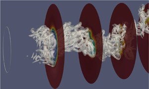
To visualise the vortex shedding structure, in figure 20 we plot the isosurfaces of the  $\lambda _{ci}$ (swirling strength) criterion in the wake (Chakraborty, Balachandar & Adrian Reference Chakraborty, Balachandar and Adrian2005). From figure 20, it can be seen that the vortical motions self-organise into a helical structure, with the packets of high swirling strength passing through the regions of low streamwise velocity, as can be seen from the cross-sectional slices in figure 20.
Helical structure in the wake visualised by  $\lambda _{ci}=5(u_{\infty }/D)^2$. The cross-sectional slices are coloured by streamwise velocity. The first slice is at
 $x=1.6D$, the separation between slices is
 $1.4D$.

To understand the motion of the helical structure in time, following Achenbach (Reference Achenbach1974) and Tomboulides & Orszag (Reference Tomboulides and Orszag2000), we calculate the correlations of fluctuating streamwise velocity among the points on a cross-sectional plane that are located at the same radial distance from the centreline and are separated by a fixed angle of  ${\rm \pi} /2$ in the azimuthal direction. The cross-correlation function is defined as
 \begin{equation} R_{ij}(x,r,\tau)=\langle u'(x,r,\theta_i,t)u'(x,r,\theta_j,t+\tau) \rangle_t, \end{equation}
where  $\theta _i$,
 $\theta _j$,
 $i,j=1,2,3,4$, are the phase angles corresponding to the four chosen probes (see figure 21 for the precise location of the probes). The auto-correlation function is obtained if
 $j=i$. The normalised correlation function is further defined as
 \begin{equation} \rho_{ij}(x,r,\tau)=\frac{R_{ij}(x,r,\tau)}{\left(R_{ii}(x,r,0)R_{jj}(x,r,0)\right)^{1/2}}. \end{equation}
Here the time series of fluctuating velocity at probe  $i$ is called event
 $i$ for brevity. If we look at
 $\rho _{12}$ and
 $\rho _{14}$ plots in figure 21(a) for
 $(x,r)=(1.4D,0.5D)$, we observe the phase angle for the events 2 and 4 being
 $\pm {\rm \pi}/2$ (the time series are shifted by
 $\pm {\rm \pi}/2$ from the event 1), coinciding with their azimuthal separation from the event 1. For
 $\rho _{13}$, the phase angle between events 1 and 3 is correspondingly
 ${\rm \pi}$, being equal to the angular difference as well. A conclusion can be drawn that there is a rotating signal on this cross-sectional plane. Similar rotating signal is also captured in the intermediate wake at
 $(x,r)=(9.8D,0.5D)$ (figure 21b). As shown in figure 17(a), the non-zero cross-sectional moment indicative of the actual rotation of the turbulent structure occurs only in the recirculation region. This rotating process in the near wake leads to a formation of the corkscrew-shaped helical structure. Upon exiting the recirculation region, the helical structure translates to the downstream area without rotation. The rotating signal on a cross-sectional plane is simply a manifestation of this translational motion of the structure, which attains a spiraling shape (see also the corresponding DMD mode in figure 9). The passing frequency of the events based on the temporal separation of the neighbouring peaks,
 $\tau _p$ (figure 21), results in
 $St=D/(\tau _p u_\infty )=0.278$, which confirms the connection of this rotational signal to the vortex shedding.
Normalised auto- and cross-correlation functions among the four probes at (a)  $(x,r)=(1.4D,0.5D)$ and (b)
 $(x,r)=(9.8D,0.5D)$. Location of the four probes is shown in (c). Images in (a,b) correspond to (from top to bottom):
 $\rho _{11}$,
 $\rho _{12}$,
 $\rho _{13}$,
 $\rho _{14}$. Here
 $\tau _p$ denotes the time period between the neighbouring peaks.

We now look at the temporal evolution of the vorticity magnitude on the slices with different azimuthal angles, as illustrated in figure 22 (please, also refer to Movie 1 in the online supplementary material available at https://doi.org/10.1017/jfm.2023.231). We can see that in each plane, the vortex packets detach from the upper and lower shear layers alternatingly. These ‘upper’ and ‘lower’ vortices form the peaks and the troughs, respectively, of the wavy structure, as seen in the streamwise-radial slices; or a skeleton of the helical structure in three dimensions. However, the same alternating pattern exists at any plane of symmetry, characterised by an arbitrary azimuthal angle, at any given time. This conclusion is corroborated by figure 22, which suggests that the same vortical structure can be tracked at equally separated azimuthal slices with a constant time delay (alternatively, constant streamwise separation at a fixed time instance).
Analysis of instantaneous vorticity magnitude  $|\omega |\, D/u_{\infty }$ on selected slices. (a) A three-dimensional position of the slices. Slice 2 is at
 $z=0$. (b) Temporal evolution of the vorticity magnitude on the three selected slices in approximately one vortex shedding cycle. The snapshots between any adjacent columns are
 $\Delta t_{snap}\,u_\infty /D=0.6$ apart. The white and yellow arrows are pointing to the peak and trough of the wavy structure (projection of the helical structure), respectively. The blue dashed line connects the peaks in the same temporal positions.

3.2.5. Discussion of the vortex shedding mode
As discussed in the introduction, the vortex shedding in the RSP mode was predominantly observed for spherical wakes (Sakamoto & Haniu Reference Sakamoto and Haniu1990; Mittal et al. Reference Mittal, Wilson and Najjar2002; Rodriguez et al. Reference Rodriguez, Borell, Lemkuhl and Oliva2011), and also in some cases of axisymmetric wakes (Gentile et al. Reference Gentile, Schrijer, Oudheusden and Scarano2016; Pavia et al. Reference Pavia, Varney, Passmore and Almond2019), although the domain of interrogation in the above two studies was too short to demonstrate the wake development downstream of the vortex shedding location ( $x/D\le 1.6$). In the current study, due to a lack of a planar symmetry in the vortex shedding modes (figure 9) and in the near-wake region (figure 10), it can be concluded that the vortex shedding occurs in the RSB mode. This is not surprising, because the RSB mode is the primary stable mode after the Hopf bifurcation (figure 1) for the blunt-edged bodies, in contrast to the RSP mode for spheres (Fabre et al. Reference Fabre, Auguste and Magnaudet2008; Meliga et al. Reference Meliga, Chomaz and Sipp2009). Vortex shedding in the RSB mode in turbulent wakes has been documented previously for disks (Yang et al. Reference Yang, Liu, Wu, Zhong and Zhang2014) and for axisymmetric bodies (Pavia et al. Reference Pavia, Varney, Passmore and Almond2019). The distinguishing feature of the RSB mode is the twisting of the vortex loops in the near wake of the body (Fabre et al. Reference Fabre, Auguste and Magnaudet2008; Bury & Jardin Reference Bury and Jardin2012), termed as the ‘Yin-Yang’ pattern in Yang et al. (Reference Yang, Liu, Wu, Zhong and Zhang2014). This twisting, or the ‘Yin-Yang’ pattern, is clearly pronounced in the DMD cross-sectional slices in figure 10, and gives the vortex shedding mode its spiraling shape, observed in figure 9.
Analysis of the base pressure on the body trailing edge reveals a strong antisymmetric mode (figures 14 and 15), as in Rigas et al. (Reference Rigas, Oxlade, Morgans and Morrison2014), Gentile et al. (Reference Gentile, Schrijer, Oudheusden and Scarano2016) and Zhu & Morrison (Reference Zhu and Morrison2021), suggesting of a presence of the SS mode in the very near wake in this flow. Given that both the RSP and RSB are the bifurcations from the SS mode, and that both RSP and RSB can be constructed as a superposition of the SS mode and the two least-stable  $m=\pm 1$ unsteady modes (Fabre et al. Reference Fabre, Auguste and Magnaudet2008; Meliga et al. Reference Meliga, Chomaz and Sipp2009), it is reasonable to conjecture that vortex shedding for both modes may originate as the shedding of the vortex loops on each side of the symmetry plane. For the RSB mode, however, the vortex loops do not stay symmetric: either during their formation or the early stages of shedding, they may experience an azimuthal shear that breaks their planar symmetry and gives them their twisted shapes. The signs of the rotational motion are indeed detected in the near wake in the current study (in the flow streamlines in figure 17(b) and in the negative mean cross-sectional moment in figure 17a). They may be an indication of the processes that are potentially triggered by an uneven pressure distribution on the base of the body (Yun et al. Reference Yun, Kim and Choi2006; Rigas et al. Reference Rigas, Oxlade, Morgans and Morrison2014) due to a symmetry breaking. We remark that these rotational processes only occur in the recirculation bubble in the current work. This is in remarkable agreement with the analytical study by Meliga et al. (Reference Meliga, Chomaz and Sipp2009) who showed that the nonlinear interactions between the modes only occur in the recirculation bubble and named this region the ‘effective wavemaker’. In this sense, the near-wake processes shape the coherent structures, which subsequently shed and translate into the intermediate wake, producing the rotating signals in the cross-sectional planes without an actual rotation. Rotating signals on the cross-sectional planes have also been recorded for spheres (Achenbach Reference Achenbach1974; Tomboulides & Orszag Reference Tomboulides and Orszag2000; Yun et al. Reference Yun, Kim and Choi2006), and similar mechanisms may be at play in these cases (Yun et al. Reference Yun, Kim and Choi2006).
The VLF motions are related to a destabilisation of the SS mode by turbulent fluctuations. This is supported by previous studies that demonstrated a good agreement between stochastic diffusive models as applied to a steady bifurcated mode and experimental data of the VLF dynamics in bluff-body wakes (Rigas et al. Reference Rigas, Morgans, Brackston and Morrison2015) and Rayleigh–Bénard convection (Brown & Ahlers Reference Brown and Ahlers2008). The presented data supports this hypothesis. As the VLF dynamics is related to the SS mode, it can occur with both the RSP shedding as documented previously (Rigas et al. Reference Rigas, Oxlade, Morgans and Morrison2014; Gentile et al. Reference Gentile, Schrijer, Oudheusden and Scarano2016), and with the RSB shedding. In the RSB mode, it is responsible for a stochastic azimuthal meandering of the vortex shedding plane with respect to an initial orientation of the Yin-Yang structure, as seen from the near-wake barycentre dynamics (figure 11). Another aspect of the VLF motion is the radial ‘breathing’, or flapping of the shear layer (Wolf et al. Reference Wolf, Klei, Buffo, Hörnschemeyer and Stumpf2012; Gentile et al. Reference Gentile, Schrijer, Oudheusden and Scarano2016), which may be related to a destabilisation of the  $|m|=2$ mode (see modes 4 and 5 of the base pressure in figure 15). This is suggested by the shape of the VLF mode in the intermediate wake, after the rotational effects of the recirculation region are diminished, which has a clear
 $|m|=2$ shape (figures 9 and 10). Future studies are needed to further clarify the mechanisms of azimuthal versus radial VLF motions in bluff-body wakes.
4. Conclusions
The current paper presents the results of a DNS of a turbulent wake past a body of revolution with a blunt trailing edge at Reynolds number  $Re=5000$. The simulations are run for over 1000 vortex shedding cycles, and the statistics is collected for approximately 800 shedding cycles in order to capture the VLF motions.
Three systems of coherent motions are detected and investigated for the current wake flow: VLF motions with  $St\sim 0.002- 0.005$ originating in the near wake, the bubble pumping motion with
 $St=0.02$ in the recirculation region and the vortex shedding motion with
 $St=0.27$ associated with the shedding of large-scale vortex structures in the shear layer and into the wake. The VLF motion is potentially associated with a stochastic destabilisation of the SS mode (Rigas et al. Reference Rigas, Morgans, Brackston and Morrison2015) and displays both azimuthal (
 $St\sim 0.002$) and radial (
 $St\sim 0.005$) dynamics. The bubble pumping motion was found to be localised primarily in the recirculation region and was attributed to the Görtler instability of the curved streamlines in the separation bubble (Wu et al. Reference Wu, Meneveau and Mittal2020; Hu et al. Reference Hu, Hickel and Van Oudheusden2021). Vortex shedding mode is the strongest mode felt both in the near and in the intermediate wake of the flow. Vortex shedding in the RSB mode (Fabre et al. Reference Fabre, Auguste and Magnaudet2008; Bury & Jardin Reference Bury and Jardin2012; Yang et al. Reference Yang, Liu, Wu, Zhong and Zhang2014) was observed in the current flow, which resulted in a twisting of the detaching vortex loops in the backflow region and their subsequent convection into the intermediate wake, giving the vortex shedding mode a characteristic spiraling shape. A double vortex shedding mode, with
 $St=0.55$, in the form of a double helix, was also detected, potentially emerging as a structure that reflects the passing of both positively and negatively oriented vortex loops.
It was found that the critical processes that shape the wake structure occur in the recirculation region, including a low-frequency reorientation of the vortex shedding plane, low-frequency meandering of a radial barycentre position and twisting of the vortex loops. These processes form the vortex shedding structure, which subsequently convects to the intermediate wake and radially diffuses outwards. In this sense, there is a strong connection between the near- and the intermediate-wake motions. Vortex shedding frequency is detectable in the base pressure spectrum and downstream in the near and the intermediate wake, suggesting that the vortex shedding processes start forming upstream of the actual shedding location. VLF motions, although forming in the very near wake, are felt in the intermediate wake as well, as manifested by a persistent VLF mode in a global structure of the flow. It is however noted that only the radial VLF processes may be present in the intermediate wake, whereas the azimuthal VLF processes, associated with the lowest detected frequency of  $St=0.002$, are localised in the near-wake region. In addition, the bubble pumping motion, manifesting as an axisymmetric
 $m=0$ mode, was found to be primarily confined to the recirculation region of the flow.
The presented information of the low-dimensional structure of the turbulent wake behind an axisymmetric bluff body can be useful for developing low-order models of the wake dynamics. It can also help design control interventions to reduce the undesirable effects of the flow separation and the associated unsteady motions, such as a high drag on the body (Beaudoin et al. Reference Beaudoin, Cadot, Aider and Wesfreid2006; Pastoor et al. Reference Pastoor, Henning, Noack, King and Tadmor2008), an increased acoustic noise (Cattafesta et al. Reference Cattafesta III, Song, Williams, Rowley and Alvi2008; Das Gupta & Roy Reference Das Gupta and Roy2015) and aero-optical distortions (Fitzgerald & Jumper Reference Fitzgerald and Jumper2004; Smith, Gordeyev & Jumper Reference Smith, Gordeyev and Jumper2011).
Supplementary movie
Supplementary movie is available at https://doi.org/10.1017/jfm.2023.231.
Funding
This work has been supported by NSF grants CBET-1707075 and CAREER-1944568. The computational time has been provided by NSF XSEDE supercomputing resources.
Declaration of interests
The authors report no conflict of interest.
Appendix A. Grid resolution comparison
In table 2, we compare the grid resolution and the statistical averaging time with the other DNS studies of wake flows at comparable Reynolds numbers. In this table,  $N_{{ptv}}$ is the number of points in the viscous sublayer, averaged along the surface of the body. We also compute the averaged grid-point distances
 $\bar {h}_{nw}/D$,
 $\bar {h}_{iw}/D$, respectively, in the near wake (
 $0\le x\le 1.6D$) and the intermediate wake (
 $x\ge 1.6D$) of the model, where
 $x=0$ corresponds to the trailing edge of the body. More precisely,
 $\bar {h}_{nw}$,
 $\bar {h}_{iw}$ are defined as the averaged grid-point distances over all the elements residing in a cylindrical volume around the grid centreline with a radius of
 $D/2$ and a streamwise length corresponding to a particular region in the wake, such as
 \begin{equation} \left. \begin{aligned} \bar{h}_{nw} & = \frac{\Bigg(\displaystyle\sum_e V_e\Bigg)^{1/3}}{N_{enw}\,N}\big| \{e:[\min x(e),\max x(e)]\subset[0,1.6D], \max r(e)\le D/2\},\\ \bar{h}_{iw} & = \frac{\Bigg(\displaystyle\sum_e V_e\Bigg)^{1/3}}{N_{eiw}\,N}\big| \{e:[\min x(e),\max x(e)]\subset[1.6D,20D], \max r(e)\le D/2\}, \end{aligned} \right\} \end{equation}
where  $N_{enw}$,
 $N_{inw}$ are the corresponding number of elements within the cylindrical volume defined for the near- and intermediate-wake regions, respectively,
 $V_e$ is the element volume. Grid-point distances
 $\bar {h}_{nw}$,
 $\bar {h}_{iw}$ are evaluated based on the velocity grid, so that
 $N=7$ is taken in (A1). While comparing
 $\bar {h}_{nw}/D$,
 $\bar {h}_{iw}/D$ with the finite-grid or finite-volume approaches in table 2, the definition (A1) is adjusted to correspond to the cell volumes instead of the element volumes, and division by
 $N$ is omitted. We should also note that the definitions of the near-wake and the intermediate-wake regions are based on the length of the separation bubble, which is case-dependent. From table 2, the current DNS grid is as fine as or finer than the grids employed in previously published computations, and the current DNS simulation runs for a significantly longer time.
Grid resolution and time-averaging parameters in comparison with other DNS of wake flows. Dashes indicate that the data are not available. The last line in the table corresponds to a statistical averaging time in terms of vortex shedding cycles.

Appendix B. Validation of the numerical methodology
To validate our numerical set-up and the solver capabilities in application to flows over bluff bodies, we performed an auxiliary DNS for a flow over a sphere at  $Re=3700$, which was investigated previously via DNS (Rodriguez et al. Reference Rodriguez, Borell, Lemkuhl and Oliva2011; Bazilevs et al. Reference Bazilevs, Yan, De Stadler and Sarkar2014; Dorschner et al. Reference Dorschner, Frapolli, Chikatamarla and Karlin2016; Pal et al. Reference Pal, Sarkar, Posa and Balaras2017) and via experiments (Kim & Durbin Reference Kim and Durbin1988). Note that we are unable to perform a validation in the context of the original geometry of a cylindrical body of revolution, because all the previous studies [experiments (Jiménez et al. Reference Jiménez, Hultmark and Smits2010; Rigas et al. Reference Rigas, Oxlade, Morgans and Morrison2014; Ashok et al. Reference Ashok, Buren and Smits2015; Gentile et al. Reference Gentile, Schrijer, Oudheusden and Scarano2016; Pavia et al. Reference Pavia, Varney, Passmore and Almond2019) or large eddy simulations (Posa & Balaras Reference Posa and Balaras2016; Kumar & Mahesh Reference Kumar and Mahesh2018; Zhu & Morrison Reference Zhu and Morrison2021)] were performed with significantly higher Reynolds numbers unaccessible by DNS. For a flow over a sphere, a series of four meshes and their resolution parameters used for the validation studies are listed in table 3. The numerical method, initial and boundary conditions remain the same as for the body of revolution. A comparison of the vortex shedding Strouhal number (
 $St$), the length of the separation bubble (
 $L_{sep}/D$), the drag coefficient on the body surface (
 $C_{d}$) and the separation angle (
 $\varphi _{sep}$) with the available data from the literature can be found in table 4. A comparison of the pressure coefficient,
 $C_{p}$, and skin friction coefficient,
 $\tau _{w}/(\rho u_\infty ^2 Re^{-0.5})$,
 $\rho$ is the fluid density, over the sphere surface is illustrated in figure 23. Mean streamwise velocity profiles at several axial locations along the wake are compared in figure 24. The presented data demonstrates that grid convergence is achieved at a resolution level comparable to that of the mesh employed for the DNS of the ogive cylinder, and shows a good agreement with the previously published data.
Validation of DNS with Nek5000 for a flow over a sphere at  $Re=3700$: (a) pressure coefficient,
 $C_{p}$, along the sphere surface; (b) skin-friction coefficient,
 $\tau _{w}/(\rho u_\infty ^2 Re^{-0.5})$, along the sphere surface. Angle
 $\varphi$ is along the circumference of the sphere, counted from the stagnation point, in degrees.

Validation of DNS with Nek5000 for a flow over a sphere at  $Re=3700$. Time-averaged streamwise velocity profiles at (a)
 $x/D=0.2$, (b)
 $x/D=1.6$ and (c)
 $x/D=3$. The centre of the sphere is at (0,0,0).

Grid resolution and time-averaging parameters for a DNS validation case for a flow over a sphere at  $Re=3700$ with Nek5000 (Zhang & Peet Reference Zhang and Peet2022). Near wake for a sphere is defined as
 $0\le x\le 3D$ and intermediate wake is at
 $3D\le x\le 5D$. DOF denotes the total number of degrees of freedom.

Comparison of  $St$,
 $L_{sep}/D$,
 $C_{d}$ and
 $\varphi _{sep}$ for a flow over a sphere at
 $Re=3700$ between Nek5000 and other available data. LBM denotes lattice Boltzmann method. Dashes indicate that the data are not available.


 Open access

