1 Introduction
Circular Couette flow of a viscous Newtonian fluid between two coaxial differentially rotating cylinders is a canonical system for modelling instabilities leading to spatio-temporal patterns and transition to turbulence in many natural and industrial processes. Modern astrophysical applications require understanding of basic instability mechanisms in rotating flows with the Keplerian shear profile in accretion- and protoplanetary disks that are hydrodynamically stable according to the centrifugal Rayleigh criterion. Usually, these instabilities are a consequence of additional factors such as electrical conductivity of the fluid and the magnetic field of the central gravitating object (Chandrasekhar Reference Chandrasekhar1961; Lifshitz Reference Lifshitz1987; Friedlander & Vishik Reference Friedlander and Vishik1995; Urpin & Brandenburg Reference Urpin and Brandenburg1998; Kucherenko & Kryvko Reference Kucherenko and Kryvko2013; Kirillov, Stefani & Fukumoto Reference Kirillov, Stefani and Fukumoto2014; Child, Kersalé & Hollerbach Reference Child, Kersalé and Hollerbach2015; Balbus & Potter Reference Balbus and Potter2016). However, in the so-called ‘dead-zones’ of protoplanetary disks that are characterized by high electrical resistivity due to very low ionization levels, some magnetohydrodynamic (MHD) instabilities become inefficient (e.g. the standard Velikhov–Chandrasekhar magnetorotational instability (MRI) in an axial magnetic field). Alternative mechanisms include MRIs caused by azimuthal or helical magnetic fields that work well also in the inductionless limit at a very low conductivity (Kirillov & Stefani Reference Kirillov and Stefani2013; Kirillov et al. Reference Kirillov, Stefani and Fukumoto2014) as well as pure hydrodynamic finite-amplitude nonlinear instabilities (Marcus et al. Reference Marcus, Pei, Jiang and Hassanzadeh2013). Some recent studies indicated a possibility that Keplerian disks with strong mean radial temperature gradients can support the so-called Goldreich–Schubert–Fricke (GSF) instability, which is the instability of short-radial-wavelength inertial modes (Economides & Moir Reference Economides and Moir1980; Urpin & Brandenburg Reference Urpin and Brandenburg1998; Nelson, Gressel & Umurhan Reference Nelson, Gressel and Umurhan2013; Balbus & Potter Reference Balbus and Potter2016). These astrophysical implications renewed interest in the effect of radial temperature gradients on the stability of circular Couette flow and its observation in the laboratory (Yoshikawa, Nagata & Mutabazi Reference Yoshikawa, Nagata and Mutabazi2013; Meyer, Yoshikawa & Mutabazi Reference Meyer, Yoshikawa and Mutabazi2015).
Typically, instabilities in circular Couette flow are studied numerically, for instance, via normal mode analysis or direct numerical simulations. An alternative technique developed in the literature (Eckhoff Reference Eckhoff1981; Lifshitz Reference Lifshitz1987; Lifschitz Reference Lifschitz1991; Lifschitz & Hameiri Reference Lifschitz and Hameiri1991; Dobrokhotov & Shafarevich Reference Dobrokhotov and Shafarevich1992; Lifschitz & Hameiri Reference Lifschitz and Hameiri1993; Eckhardt & Yao Reference Eckhardt and Yao1995; Friedlander & Vishik Reference Friedlander and Vishik1995) is based on perturbations of a background flow in a small parameter, representing a short wavelength, as in geometric optics (Lifschitz, Suters & Beale Reference Lifschitz, Suters and Beale1996). These perturbations are localized wave envelopes moving along the trajectories of fluid elements. The flow is unstable if the amplitude of the envelope demonstrates an unbounded growth in time along at least one trajectory.
The geometric optics stability analysis requires the representation of the solution to the governing equations linearized about the background flow as a generalized progressive wave expansion (Eckhoff Reference Eckhoff1981). Since the leading-order term in this expansion dominates the solution for a sufficiently long time, provided that the short-wavelength parameter is small enough, it is sufficient for detecting instability to determine the growth rate of the lowest-order amplitude (Eckhoff Reference Eckhoff1981; Lifschitz Reference Lifschitz1991). The growth rates are given by the real parts of the roots of the dispersion relation of the linear transport equation for the lowest-order amplitude that depends on the wave vector of the perturbation. The wave vector evolves along a stream line of the flow and this evolution is governed by an eikonal equation. The stream line passing through a particular point fulfils a corresponding trajectory equation. Thus, detecting instabilities localized near a particular fluid element location, moving with the flow, reduces to solving a system of ordinary differential equations for the wave vector and amplitude, along particle paths in the underlying flow, with coefficients depending on the unperturbed velocity field (Lifschitz et al. Reference Lifschitz, Suters and Beale1996).
The geometric optics stability analysis has proved successful in solving problems of ideal hydrodynamics and magnetohydrodynamics related to the stability of rotating flows of an incompressible fluid (Eckhoff Reference Eckhoff1981; Lifshitz Reference Lifshitz1987; Lifschitz Reference Lifschitz1991; Lifschitz & Hameiri Reference Lifschitz and Hameiri1991, Reference Lifschitz and Hameiri1993; Friedlander & Vishik Reference Friedlander and Vishik1995; Lifschitz et al. Reference Lifschitz, Suters and Beale1996; Kucherenko & Kryvko Reference Kucherenko and Kryvko2013). It was extended to the viscous and resistive cases in Lifschitz (Reference Lifschitz1991), Dobrokhotov & Shafarevich (Reference Dobrokhotov and Shafarevich1992), Eckhardt & Yao (Reference Eckhardt and Yao1995), Kirillov (Reference Kirillov2013), Kirillov et al. (Reference Kirillov, Stefani and Fukumoto2014), Allilueva & Shafarevich (Reference Allilueva and Shafarevich2015). In particular, this technique allowed one to find analytically neutral stability surfaces in the parameter space, the frequencies of the unstable modes and their growth rates, that agreed well with the numerical simulations (Eckhardt & Yao Reference Eckhardt and Yao1995; Lifschitz et al. Reference Lifschitz, Suters and Beale1996; Kirillov et al. Reference Kirillov, Stefani and Fukumoto2014; Child et al. Reference Child, Kersalé and Hollerbach2015; Stefani & Kirillov Reference Stefani and Kirillov2015).
In this paper we apply the geometric optics stability analysis to circular Couette flow of a viscous Newtonian fluid with a temperature gradient in the absence of gravity, but retaining the term of the centrifugal buoyancy. We derive a system of characteristic equations that includes the transport equations for the lowest-order amplitude of the envelope of the localized perturbation and find a dispersion relation that takes into account the radial variation of the angular velocity and the temperature as well as the kinematic viscosity and the thermal diffusivity.
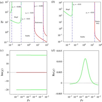
Using algebraic stability criteria for localization of the roots of polynomials in the left half of the complex plane, we obtain two stability conditions in compact and explicit form; one of them generalizes the Rayleigh discriminant for stationary axisymmetric instabilities to include viscosity effects, and the other provides a marginal stability curve in the parameter plane for oscillatory instabilities. Codimension-2 points on the marginal stability thresholds are identified and the growth rates and frequencies of the instabilities are found analytically. The theoretical results are applied to cylindrical Couette flow with the parameters evaluated at the geometric mean radius both in the Rayleigh unstable and in the Rayleigh stable regimes. In the case of a sole inner cylinder rotating we confirm and extend the numerical results of Meyer et al. (Reference Meyer, Yoshikawa and Mutabazi2015) and provide analytical expressions for the onset of oscillatory and stationary instabilities, the coordinates of the codimension-2 points, and the Hopf frequency. In the case of a sole outer cylinder rotation, solid body rotation, and rotating flow with Keplerian shear we find a destabilizing effect of the inward temperature gradient that leads to oscillatory instability at small values of the Prandtl number (
 $Pr<1$
) and to stationary instability at
 $Pr>1$
.
2 Equations of motion
We consider the flow of an incompressible viscous fluid of density
 $\unicode[STIX]{x1D70C}$
, kinematic viscosity
 $\unicode[STIX]{x1D708}$
and thermal diffusivity
 $\unicode[STIX]{x1D705}$
in the presence of a radial temperature gradient applied to a differentially rotating cylindrical annulus. The ratio
 $Pr=\unicode[STIX]{x1D708}/\unicode[STIX]{x1D705}$
constitutes the Prandtl number.
The governing equations written in the inertial frame of reference read (Yoshikawa et al. Reference Yoshikawa, Nagata and Mutabazi2013; Meyer et al. Reference Meyer, Yoshikawa and Mutabazi2015):
 $$\begin{eqnarray}\displaystyle & \displaystyle \unicode[STIX]{x1D735}\boldsymbol{\cdot }\boldsymbol{u}=0, & \displaystyle\end{eqnarray}$$
 $$\begin{eqnarray}\displaystyle & \displaystyle \frac{\unicode[STIX]{x2202}\boldsymbol{u}}{\unicode[STIX]{x2202}t}+\boldsymbol{u}\boldsymbol{\cdot }\unicode[STIX]{x1D735}\boldsymbol{u}+\frac{1}{\unicode[STIX]{x1D70C}}\unicode[STIX]{x1D735}p-\unicode[STIX]{x1D708}\unicode[STIX]{x0394}\boldsymbol{u}+\unicode[STIX]{x1D6FC}\unicode[STIX]{x1D703}\boldsymbol{g}_{c}=0, & \displaystyle\end{eqnarray}$$
 $$\begin{eqnarray}\displaystyle & \displaystyle \frac{\unicode[STIX]{x2202}\unicode[STIX]{x1D703}}{\unicode[STIX]{x2202}t}+\boldsymbol{u}\boldsymbol{\cdot }\unicode[STIX]{x1D735}\unicode[STIX]{x1D703}-\unicode[STIX]{x1D705}\unicode[STIX]{x0394}\unicode[STIX]{x1D703}=0, & \displaystyle\end{eqnarray}$$
where
 $p$
is the pressure and
 $\unicode[STIX]{x1D703}$
is the temperature deviation from a reference temperature. The parameter
 $\unicode[STIX]{x1D6FC}$
is the coefficient of thermal expansion.
The flow equations are written in cylindrical coordinates
 $(r,\unicode[STIX]{x1D711},z)$
in which the velocity field
 $\boldsymbol{u}=(u,v,w)^{\text{T}}$
, where the superscript
 $T$
denotes transposition. The term
 $\boldsymbol{u}\boldsymbol{\cdot }\unicode[STIX]{x1D735}\boldsymbol{u}$
contains the centrifugal-like acceleration
 $\boldsymbol{g}_{c}=(v^{2}/r,0,0)^{\text{T}}$
and the Coriolis-like acceleration
 $(0,uv/r,0)^{\text{T}}$
coming from the geometry. The Oberbeck–Boussinesq approximation (Chandrasekhar Reference Chandrasekhar1961) is used, i.e. we assume small variations of the density with temperature only in the centrifugal force term leading to the centrifugal buoyancy while the other fluid properties (
 $\unicode[STIX]{x1D708},\unicode[STIX]{x1D705},\unicode[STIX]{x1D6FC}$
) are kept constant. This approximation allows one to keep the flow incompressibility condition and eliminates the acoustic modes from the problem analysis. The application of the Oberbeck–Boussinesq approximation to rotating flows can be found in Lopez, Marques & Avila (Reference Lopez, Marques and Avila2013). The gravity
 $g$
is neglected in order to focus only on the destabilization effects of the centrifugal buoyancy
 $\unicode[STIX]{x1D6FC}\unicode[STIX]{x1D703}\boldsymbol{g}_{c}$
.
We assume that the cylindrical annulus has an infinite length. The system (2.1)–(2.3) possesses a stationary axisymmetric solution describing the base flow state:
 $\boldsymbol{u}_{B}=(0,V(r)=r\unicode[STIX]{x1D6FA}(r),0)^{\text{T}}$
,
 $p_{B}=P(r)$
, and
 $\unicode[STIX]{x1D703}_{B}=\unicode[STIX]{x1D6E9}(r)$
. Consider a perturbation of this base flow state:
 $\boldsymbol{u}=\boldsymbol{u}_{B}+\widetilde{\boldsymbol{u}}$
,
 $p=p_{B}+\widetilde{p}$
, and
 $\unicode[STIX]{x1D703}=\unicode[STIX]{x1D703}_{B}+\widetilde{\unicode[STIX]{x1D703}}$
. Then the equations of the flow perturbations linearized around the base flow state read
 $$\begin{eqnarray}\displaystyle & \displaystyle \unicode[STIX]{x1D735}\boldsymbol{\cdot }\widetilde{\boldsymbol{u}}=0, & \displaystyle\end{eqnarray}$$
 $$\begin{eqnarray}\displaystyle & \displaystyle \frac{\unicode[STIX]{x2202}\widetilde{\boldsymbol{u}}}{\unicode[STIX]{x2202}t}+\boldsymbol{u}_{B}\boldsymbol{\cdot }\unicode[STIX]{x1D735}\widetilde{\boldsymbol{u}}+\widetilde{\boldsymbol{u}}\boldsymbol{\cdot }\unicode[STIX]{x1D735}\boldsymbol{u}_{B}-\unicode[STIX]{x1D708}\unicode[STIX]{x0394}\widetilde{\boldsymbol{u}}+\frac{1}{\unicode[STIX]{x1D70C}}\unicode[STIX]{x1D735}\widetilde{p}+\unicode[STIX]{x1D6FC}\unicode[STIX]{x1D703}_{B}\widetilde{\boldsymbol{g}}_{c}+\unicode[STIX]{x1D6FC}\widetilde{\unicode[STIX]{x1D703}}\boldsymbol{g}_{cB}=0, & \displaystyle\end{eqnarray}$$
 $$\begin{eqnarray}\displaystyle & \displaystyle \frac{\unicode[STIX]{x2202}\widetilde{\unicode[STIX]{x1D703}}}{\unicode[STIX]{x2202}t}+\boldsymbol{u}_{B}\boldsymbol{\cdot }\unicode[STIX]{x1D735}\widetilde{\unicode[STIX]{x1D703}}+\widetilde{\boldsymbol{u}}\boldsymbol{\cdot }\unicode[STIX]{x1D735}\unicode[STIX]{x1D703}_{B}-\unicode[STIX]{x1D705}\unicode[STIX]{x0394}\widetilde{\unicode[STIX]{x1D703}}=0, & \displaystyle\end{eqnarray}$$
with the basic centrifugal gravity
 $\boldsymbol{g}_{cB}=(r\unicode[STIX]{x1D6FA}^{2},0,0)^{\text{T}}$
and the perturbative centrifugal gravity
 $\widetilde{\boldsymbol{g}}_{c}=(2\unicode[STIX]{x1D6FA}\widetilde{v},0,0)^{\text{T}}$
so that we can write the centrifugal buoyancy terms as follows
 $$\begin{eqnarray}\displaystyle & \displaystyle \unicode[STIX]{x1D6FC}\unicode[STIX]{x1D703}_{B}\widetilde{\boldsymbol{g}}_{c}=2\unicode[STIX]{x1D6FA}\unicode[STIX]{x1D6FC}\unicode[STIX]{x1D703}_{B}\boldsymbol{e}_{r}\boldsymbol{e}_{\unicode[STIX]{x1D711}}^{\text{T}}\widetilde{\boldsymbol{u}}, & \displaystyle\end{eqnarray}$$
 $$\begin{eqnarray}\displaystyle & \displaystyle \unicode[STIX]{x1D6FC}\widetilde{\unicode[STIX]{x1D703}}\boldsymbol{g}_{cB}=\unicode[STIX]{x1D6FC}\widetilde{\unicode[STIX]{x1D703}}r\unicode[STIX]{x1D6FA}^{2}\boldsymbol{e}_{r}, & \displaystyle\end{eqnarray}$$
where
 $\boldsymbol{e}_{r}$
and
 $\boldsymbol{e}_{\unicode[STIX]{x1D711}}$
are radial and azimuthal unit vectors, respectively.
The gradients of the background fields are
 $$\begin{eqnarray}\unicode[STIX]{x1D735}\boldsymbol{u}_{B}=\unicode[STIX]{x1D6FA}\left(\begin{array}{@{}ccc@{}}0 & -1 & 0\\ 1+2Ro & 0 & 0\\ 0 & 0 & 0\end{array}\right),\quad \unicode[STIX]{x1D735}\unicode[STIX]{x1D703}_{B}=\left(\begin{array}{@{}c@{}}D\unicode[STIX]{x1D6E9}\\ 0\\ 0\end{array}\right),\end{eqnarray}$$
where
 $$\begin{eqnarray}Ro=\frac{rD\unicode[STIX]{x1D6FA}}{2\unicode[STIX]{x1D6FA}}\end{eqnarray}$$
is the Rossby number and
 $D=\text{d}/\text{d}r$
. Denoting
 ${\mathcal{U}}=\unicode[STIX]{x1D735}\boldsymbol{u}_{B}$
, we formulate the linearized equations of motion in the final form:
 $$\begin{eqnarray}\displaystyle & \displaystyle \unicode[STIX]{x1D735}\boldsymbol{\cdot }\widetilde{\boldsymbol{u}}=0, & \displaystyle\end{eqnarray}$$
 $$\begin{eqnarray}\displaystyle & \displaystyle \left(\frac{\unicode[STIX]{x2202}}{\unicode[STIX]{x2202}t}+{\mathcal{U}}+2\unicode[STIX]{x1D6FA}\unicode[STIX]{x1D6FC}\unicode[STIX]{x1D703}_{B}\boldsymbol{e}_{r}\boldsymbol{e}_{\unicode[STIX]{x1D711}}^{\text{T}}+\boldsymbol{u}_{B}\boldsymbol{\cdot }\unicode[STIX]{x1D735}\right)\widetilde{\boldsymbol{u}}-\unicode[STIX]{x1D708}\unicode[STIX]{x0394}\widetilde{\boldsymbol{u}}+\frac{1}{\unicode[STIX]{x1D70C}}\unicode[STIX]{x1D735}\widetilde{p}+\unicode[STIX]{x1D6FC}r\unicode[STIX]{x1D6FA}^{2}\boldsymbol{e}_{r}\widetilde{\unicode[STIX]{x1D703}}=0, & \displaystyle\end{eqnarray}$$
 $$\begin{eqnarray}\displaystyle & \displaystyle \left(\frac{\unicode[STIX]{x2202}}{\unicode[STIX]{x2202}t}+\boldsymbol{u}_{B}\boldsymbol{\cdot }\unicode[STIX]{x1D735}\right)\widetilde{\unicode[STIX]{x1D703}}+\widetilde{\boldsymbol{u}}\boldsymbol{\cdot }\unicode[STIX]{x1D735}\unicode[STIX]{x1D703}_{B}-\unicode[STIX]{x1D705}\unicode[STIX]{x0394}\widetilde{\unicode[STIX]{x1D703}}=0. & \displaystyle\end{eqnarray}$$
3 Evolution of the localized perturbations
Let
 $\unicode[STIX]{x1D716}$
be a small parameter (
 $0<\unicode[STIX]{x1D716}\ll 1$
). We are looking for a solution of the linearized equations (2.11)–(2.13) in the form of the generalized progressive wave expansions (Eckhoff Reference Eckhoff1981)
 $$\begin{eqnarray}\displaystyle & \displaystyle \widetilde{\boldsymbol{u}}=\left(\boldsymbol{u}^{(0)}(\boldsymbol{x},t)+\unicode[STIX]{x1D716}\boldsymbol{u}^{(1)}(\boldsymbol{x},t)\right)\exp \left(\text{i}\unicode[STIX]{x1D716}^{-1}\unicode[STIX]{x1D6F7}(\boldsymbol{x},t)\right)+\unicode[STIX]{x1D716}\boldsymbol{u}^{(r)}(\boldsymbol{x},t,\unicode[STIX]{x1D716}), & \displaystyle\end{eqnarray}$$
 $$\begin{eqnarray}\displaystyle & \displaystyle \widetilde{\unicode[STIX]{x1D703}}=\left(\unicode[STIX]{x1D703}^{(0)}(\boldsymbol{x},t)+\unicode[STIX]{x1D716}\unicode[STIX]{x1D703}^{(1)}(\boldsymbol{x},t)\right)\exp \left(\text{i}\unicode[STIX]{x1D716}^{-1}\unicode[STIX]{x1D6F7}(\boldsymbol{x},t)\right)+\unicode[STIX]{x1D716}\unicode[STIX]{x1D703}^{(r)}(\boldsymbol{x},t,\unicode[STIX]{x1D716}), & \displaystyle\end{eqnarray}$$
 $$\begin{eqnarray}\displaystyle & \displaystyle \widetilde{p}=\left(p^{(0)}(\boldsymbol{x},t)+\unicode[STIX]{x1D716}p^{(1)}(\boldsymbol{x},t)\right)\exp \left(\text{i}\unicode[STIX]{x1D716}^{-1}\unicode[STIX]{x1D6F7}(\boldsymbol{x},t)\right)+\unicode[STIX]{x1D716}p^{(r)}(\boldsymbol{x},t,\unicode[STIX]{x1D716}), & \displaystyle\end{eqnarray}$$
where
 $\unicode[STIX]{x1D6F7}$
is generally a complex-valued scalar function that represents the phase of the wave or the eikonal and the remainder terms
 $\boldsymbol{u}^{(r)},\unicode[STIX]{x1D703}^{(r)},p^{(r)}$
are assumed to be uniformly bounded in
 $\unicode[STIX]{x1D716}$
on any fixed time interval (Eckhoff Reference Eckhoff1981; Lifschitz Reference Lifschitz1991; Lifschitz & Hameiri Reference Lifschitz and Hameiri1991, Reference Lifschitz and Hameiri1993; Lifschitz et al.
Reference Lifschitz, Suters and Beale1996).
Maslov (Reference Maslov1986) observed that high-frequency oscillations
 $\exp (\text{i}\unicode[STIX]{x1D716}^{-1}\unicode[STIX]{x1D6F7}(\boldsymbol{x},t))$
quickly die out because of viscosity unless one assumes a quadratic dependency of viscosity on the small parameter
 $\unicode[STIX]{x1D716}$
. Hence, following (Maslov Reference Maslov1986; Dobrokhotov & Shafarevich Reference Dobrokhotov and Shafarevich1992; Kirillov et al.
Reference Kirillov, Stefani and Fukumoto2014; Allilueva & Shafarevich Reference Allilueva and Shafarevich2015), we assume that
 $\unicode[STIX]{x1D708}=\unicode[STIX]{x1D716}^{2}\widetilde{\unicode[STIX]{x1D708}}$
and
 $\unicode[STIX]{x1D705}=\unicode[STIX]{x1D716}^{2}\widetilde{\unicode[STIX]{x1D705}}$
.
Substituting the asymptotic series (3.1) into the incompressibility condition (2.11) and collecting terms at
 $\unicode[STIX]{x1D716}^{-1}$
and
 $\unicode[STIX]{x1D716}^{0}$
, we find
 $$\begin{eqnarray}\displaystyle & \displaystyle \unicode[STIX]{x1D716}^{-1}:\quad \boldsymbol{u}^{(0)}\boldsymbol{\cdot }\unicode[STIX]{x1D735}\unicode[STIX]{x1D6F7}=0, & \displaystyle\end{eqnarray}$$
 $$\begin{eqnarray}\displaystyle & \displaystyle \unicode[STIX]{x1D716}^{0}:\quad \unicode[STIX]{x1D735}\boldsymbol{\cdot }\boldsymbol{u}^{(0)}+\text{i}\boldsymbol{u}^{(1)}\boldsymbol{\cdot }\unicode[STIX]{x1D735}\unicode[STIX]{x1D6F7}=0. & \displaystyle\end{eqnarray}$$
A similar procedure applied to (2.12) and (2.13) yields the two systems of equations
 $$\begin{eqnarray}\displaystyle & & \displaystyle \unicode[STIX]{x1D716}^{-1}:\quad \left(\begin{array}{@{}cc@{}}\displaystyle \frac{\unicode[STIX]{x2202}\unicode[STIX]{x1D6F7}}{\unicode[STIX]{x2202}t}+\boldsymbol{u}_{B}\boldsymbol{\cdot }\unicode[STIX]{x1D735}\unicode[STIX]{x1D6F7} & 0\\ 0 & \displaystyle \frac{\unicode[STIX]{x2202}\unicode[STIX]{x1D6F7}}{\unicode[STIX]{x2202}t}+\boldsymbol{u}_{B}\boldsymbol{\cdot }\unicode[STIX]{x1D735}\unicode[STIX]{x1D6F7}\end{array}\right)\left(\begin{array}{@{}c@{}}\boldsymbol{u}^{(0)}\\ \unicode[STIX]{x1D703}^{(0)}\end{array}\right)=-\frac{\unicode[STIX]{x1D735}\unicode[STIX]{x1D6F7}}{\unicode[STIX]{x1D70C}}\left(\begin{array}{@{}c@{}}p^{(0)}\\ 0\end{array}\right),\end{eqnarray}$$
 $$\begin{eqnarray}\displaystyle & & \displaystyle \unicode[STIX]{x1D716}^{0}:\quad \text{i}\left(\begin{array}{@{}cc@{}}\displaystyle \frac{\unicode[STIX]{x2202}\unicode[STIX]{x1D6F7}}{\unicode[STIX]{x2202}t}+\boldsymbol{u}_{B}\boldsymbol{\cdot }\unicode[STIX]{x1D735}\unicode[STIX]{x1D6F7} & 0\\ 0 & \displaystyle \frac{\unicode[STIX]{x2202}\unicode[STIX]{x1D6F7}}{\unicode[STIX]{x2202}t}+\boldsymbol{u}_{B}\boldsymbol{\cdot }\unicode[STIX]{x1D735}\unicode[STIX]{x1D6F7}\end{array}\right)\left(\begin{array}{@{}c@{}}\boldsymbol{u}^{(1)}\\ \unicode[STIX]{x1D703}^{(1)}\end{array}\right)=-\text{i}\frac{\unicode[STIX]{x1D735}\unicode[STIX]{x1D6F7}}{\unicode[STIX]{x1D70C}}\left(\begin{array}{@{}c@{}}p^{(1)}\\ 0\end{array}\right)\nonumber\\ \displaystyle & & \displaystyle \qquad -\,\left(\begin{array}{@{}cc@{}}\displaystyle \frac{\unicode[STIX]{x2202}}{\unicode[STIX]{x2202}t}+\boldsymbol{u}_{B}\boldsymbol{\cdot }\unicode[STIX]{x1D735}+{\mathcal{U}}+\widetilde{\unicode[STIX]{x1D708}}(\unicode[STIX]{x1D735}\unicode[STIX]{x1D6F7})^{2} & 0\\ 0 & \displaystyle \frac{\unicode[STIX]{x2202}}{\unicode[STIX]{x2202}t}+\boldsymbol{u}_{B}\boldsymbol{\cdot }\unicode[STIX]{x1D735}+\widetilde{\unicode[STIX]{x1D705}}(\unicode[STIX]{x1D735}\unicode[STIX]{x1D6F7})^{2}\end{array}\right)\left(\begin{array}{@{}c@{}}\boldsymbol{u}^{(0)}\\ \unicode[STIX]{x1D703}^{(0)}\end{array}\right)\nonumber\\ \displaystyle & & \displaystyle \qquad -\,\left(\begin{array}{@{}cc@{}}2\unicode[STIX]{x1D6FA}\unicode[STIX]{x1D6FC}\unicode[STIX]{x1D703}_{B}\boldsymbol{e}_{r}\boldsymbol{e}_{\unicode[STIX]{x1D711}}^{\text{T}} & \unicode[STIX]{x1D6FC}r\unicode[STIX]{x1D6FA}^{2}\boldsymbol{e}_{r}\\ (\unicode[STIX]{x1D735}\unicode[STIX]{x1D703}_{B})^{\text{T}} & 0\end{array}\right)\left(\begin{array}{@{}c@{}}\boldsymbol{u}^{(0)}\\ \unicode[STIX]{x1D703}^{(0)}\end{array}\right)-\frac{\unicode[STIX]{x1D735}}{\unicode[STIX]{x1D70C}}\left(\begin{array}{@{}c@{}}p^{(0)}\\ 0\end{array}\right).\end{eqnarray}$$
The amplitudes with the superscript
 $(0)$
are contained both in (3.6) corresponding to the lowest degree of
 $\unicode[STIX]{x1D716}$
equal to
 $-1$
and in (3.7) corresponding to the degree
 $0$
. Therefore, finding the lowest-order amplitudes with the superscript
 $(0)$
requires an iterative procedure involving both (3.6) and (3.7).
Taking the dot product of the first of the equations in the system (3.6) with
 $\unicode[STIX]{x1D735}\unicode[STIX]{x1D6F7}$
under the constraint (3.4) we find that for
 $\unicode[STIX]{x1D735}\unicode[STIX]{x1D6F7}\neq 0$
 $$\begin{eqnarray}p^{(0)}=0.\end{eqnarray}$$
Under the condition (3.8) the system (3.6) has a non-trivial solution if the determinant of the
 $4\times 4$
matrix in its left-hand side is vanishing. This gives us a 4-fold characteristic root corresponding to the Hamilton–Jacobi equation
 $$\begin{eqnarray}\frac{\unicode[STIX]{x2202}\unicode[STIX]{x1D6F7}}{\unicode[STIX]{x2202}t}+\boldsymbol{u}_{B}\boldsymbol{\cdot }\unicode[STIX]{x1D735}\unicode[STIX]{x1D6F7}=0,\end{eqnarray}$$
with the initial data:
 $\unicode[STIX]{x1D6F7}(\boldsymbol{x},0)=\unicode[STIX]{x1D6F7}_{0}(\boldsymbol{x})$
.
Taking the gradient of (3.9) yields the eikonal equation (Lifschitz & Hameiri Reference Lifschitz and Hameiri1991)
 $$\begin{eqnarray}\left(\frac{\unicode[STIX]{x2202}}{\unicode[STIX]{x2202}t}+\boldsymbol{u}_{B}\boldsymbol{\cdot }\unicode[STIX]{x1D735}\right)\unicode[STIX]{x1D735}\unicode[STIX]{x1D6F7}+\unicode[STIX]{x1D735}\boldsymbol{u}_{B}\boldsymbol{\cdot }\unicode[STIX]{x1D735}\unicode[STIX]{x1D6F7}=0,\end{eqnarray}$$
with the initial condition
 $\unicode[STIX]{x1D735}\unicode[STIX]{x1D6F7}(\boldsymbol{x},0)=\unicode[STIX]{x1D735}\unicode[STIX]{x1D6F7}_{0}(\boldsymbol{x})$
. In the notation
 $\boldsymbol{k}=\unicode[STIX]{x1D735}\unicode[STIX]{x1D6F7}$
and
 $(\text{d}/\text{d}t)=(\unicode[STIX]{x2202}/\unicode[STIX]{x2202}t)+\boldsymbol{u}_{B}\boldsymbol{\cdot }\unicode[STIX]{x1D735}$
the eikonal equation (3.10) is (Lifschitz Reference Lifschitz1991)
 $$\begin{eqnarray}\frac{\text{d}\boldsymbol{k}}{\text{d}t}=-\unicode[STIX]{x1D735}\boldsymbol{u}_{B}\boldsymbol{\cdot }\boldsymbol{k}=-{\mathcal{U}}^{\text{T}}\boldsymbol{k},\end{eqnarray}$$
where
 ${\mathcal{U}}^{\text{T}}$
denotes the transposed
 $3\times 3$
matrix
 ${\mathcal{U}}$
(Eckhardt & Yao Reference Eckhardt and Yao1995).
Relations (3.8) and (3.9) allow us to reduce the system (3.7) to
 $$\begin{eqnarray}\displaystyle & \displaystyle \left(\frac{\text{d}}{\text{d}t}+{\mathcal{U}}+\widetilde{\unicode[STIX]{x1D708}}(\unicode[STIX]{x1D735}\unicode[STIX]{x1D6F7})^{2}+2\unicode[STIX]{x1D6FC}\unicode[STIX]{x1D6FA}\unicode[STIX]{x1D703}_{B}\boldsymbol{e}_{r}\boldsymbol{e}_{\unicode[STIX]{x1D711}}^{\text{T}}\right)\boldsymbol{u}^{(0)}+\unicode[STIX]{x1D6FC}r\unicode[STIX]{x1D6FA}^{2}\boldsymbol{e}_{r}\unicode[STIX]{x1D703}^{(0)}=-\frac{\text{i}\unicode[STIX]{x1D735}\unicode[STIX]{x1D6F7}}{\unicode[STIX]{x1D70C}}p^{(1)}, & \displaystyle\end{eqnarray}$$
 $$\begin{eqnarray}\displaystyle & \displaystyle (\unicode[STIX]{x1D735}\unicode[STIX]{x1D703}_{B})^{\text{T}}\boldsymbol{u}^{(0)}+\left(\frac{\text{d}}{\text{d}t}+\widetilde{\unicode[STIX]{x1D705}}(\unicode[STIX]{x1D735}\unicode[STIX]{x1D6F7})^{2}\right)\unicode[STIX]{x1D703}^{(0)}=0. & \displaystyle\end{eqnarray}$$
Multiplying (3.12) with
 $\unicode[STIX]{x1D735}\unicode[STIX]{x1D6F7}$
from the left, we isolate the pressure term
 $$\begin{eqnarray}p^{(1)}=\text{i}\unicode[STIX]{x1D70C}\frac{\unicode[STIX]{x1D735}\unicode[STIX]{x1D6F7}}{(\unicode[STIX]{x1D735}\unicode[STIX]{x1D6F7})^{2}}\boldsymbol{\cdot }\left(\left[\frac{\text{d}}{\text{d}t}+{\mathcal{U}}+2\unicode[STIX]{x1D6FC}\unicode[STIX]{x1D6FA}\unicode[STIX]{x1D703}_{B}\boldsymbol{e}_{r}\boldsymbol{e}_{\unicode[STIX]{x1D711}}^{\text{T}}\right]\boldsymbol{u}^{(0)}+\unicode[STIX]{x1D6FC}r\unicode[STIX]{x1D6FA}^{2}\boldsymbol{e}_{r}\unicode[STIX]{x1D703}^{(0)}\right).\end{eqnarray}$$
Taking into account the identity (Lifschitz & Hameiri Reference Lifschitz and Hameiri1991; Kirillov et al. Reference Kirillov, Stefani and Fukumoto2014)
 $$\begin{eqnarray}\frac{\text{d}}{\text{d}t}(\unicode[STIX]{x1D735}\unicode[STIX]{x1D6F7}\boldsymbol{\cdot }\boldsymbol{u}^{(0)})=\frac{\text{d}\unicode[STIX]{x1D735}\unicode[STIX]{x1D6F7}}{\text{d}t}\boldsymbol{\cdot }\boldsymbol{u}^{(0)}+\unicode[STIX]{x1D735}\unicode[STIX]{x1D6F7}\boldsymbol{\cdot }\frac{\text{d}\boldsymbol{u}^{(0)}}{\text{d}t}=0\end{eqnarray}$$
we modify (3.14) in the following way
 $$\begin{eqnarray}p^{(1)}=\text{i}\unicode[STIX]{x1D70C}\frac{\unicode[STIX]{x1D735}\unicode[STIX]{x1D6F7}}{(\unicode[STIX]{x1D735}\unicode[STIX]{x1D6F7})^{2}}\boldsymbol{\cdot }\left(({\mathcal{U}}+2\unicode[STIX]{x1D6FC}\unicode[STIX]{x1D6FA}\unicode[STIX]{x1D703}_{B}\boldsymbol{e}_{r}\boldsymbol{e}_{\unicode[STIX]{x1D711}}^{\text{T}})\boldsymbol{u}^{(0)}+\unicode[STIX]{x1D6FC}r\unicode[STIX]{x1D6FA}^{2}\boldsymbol{e}_{r}\unicode[STIX]{x1D703}^{(0)}\right)-\text{i}\unicode[STIX]{x1D70C}\frac{1}{(\unicode[STIX]{x1D735}\unicode[STIX]{x1D6F7})^{2}}\frac{\text{d}\unicode[STIX]{x1D735}\unicode[STIX]{x1D6F7}}{\text{d}t}\boldsymbol{\cdot }\boldsymbol{u}^{(0)}.\end{eqnarray}$$
Now using (3.11) we re-write (3.16) in terms of the wave vector
 $\boldsymbol{k}$
 $$\begin{eqnarray}p^{(1)}=2\text{i}\unicode[STIX]{x1D70C}\unicode[STIX]{x1D6FC}\unicode[STIX]{x1D6FA}\unicode[STIX]{x1D703}_{B}\frac{\boldsymbol{k}^{\text{T}}\boldsymbol{e}_{r}\boldsymbol{e}_{\unicode[STIX]{x1D711}}^{\text{T}}}{|\boldsymbol{k}|^{2}}\boldsymbol{u}^{(0)}+\text{i}\unicode[STIX]{x1D70C}\unicode[STIX]{x1D6FC}r\unicode[STIX]{x1D6FA}^{2}\frac{\boldsymbol{k}^{\text{T}}\boldsymbol{e}_{r}}{|\boldsymbol{k}|^{2}}\unicode[STIX]{x1D703}^{(0)}+2\text{i}\unicode[STIX]{x1D70C}\frac{\boldsymbol{k}^{\text{T}}{\mathcal{U}}}{|\boldsymbol{k}|^{2}}\boldsymbol{u}^{(0)}.\end{eqnarray}$$
Substituting (3.17) into (3.12) we finally arrive at the transport equations for the leading-order amplitudes
 $\boldsymbol{u}^{(0)}$
and
 $\unicode[STIX]{x1D703}^{(0)}$
in the expansions (3.1) and (3.2):
 $$\begin{eqnarray}\displaystyle \frac{\text{d}\boldsymbol{u}^{(0)}}{\text{d}t} & = & \displaystyle -\widetilde{\unicode[STIX]{x1D708}}|\boldsymbol{k}|^{2}\boldsymbol{u}^{(0)}-\left({\mathcal{I}}-2\frac{\boldsymbol{k}\boldsymbol{k}^{\text{T}}}{|\boldsymbol{k}|^{2}}\right){\mathcal{U}}\boldsymbol{u}^{(0)}-2\unicode[STIX]{x1D6FC}\unicode[STIX]{x1D6FA}\unicode[STIX]{x1D703}_{B}\left({\mathcal{I}}-\frac{\boldsymbol{k}\boldsymbol{k}^{\text{T}}}{|\boldsymbol{k}|^{2}}\right)\boldsymbol{e}_{r}\boldsymbol{e}_{\unicode[STIX]{x1D711}}^{\text{T}}\boldsymbol{u}^{(0)}\nonumber\\ \displaystyle & & \displaystyle -\unicode[STIX]{x1D6FC}r\unicode[STIX]{x1D6FA}^{2}\left({\mathcal{I}}-\frac{\boldsymbol{k}\boldsymbol{k}^{\text{T}}}{|\boldsymbol{k}|^{2}}\right)\boldsymbol{e}_{r}\unicode[STIX]{x1D703}^{(0)},\end{eqnarray}$$
 $$\begin{eqnarray}\displaystyle \frac{\text{d}\unicode[STIX]{x1D703}^{(0)}}{\text{d}t}=-\widetilde{\unicode[STIX]{x1D705}}|\boldsymbol{k}|^{2}\unicode[STIX]{x1D703}^{(0)}-(\unicode[STIX]{x1D735}\unicode[STIX]{x1D703}_{B})^{\text{T}}\boldsymbol{u}^{(0)}, & & \displaystyle\end{eqnarray}$$
with
 ${\mathcal{I}}$
the
 $3\times 3$
identity matrix and the initial data
 $\boldsymbol{u}^{(0)}(\boldsymbol{x},0)=\boldsymbol{u}_{0}^{(0)}(\boldsymbol{x})$
and
 $\unicode[STIX]{x1D703}^{(0)}(\boldsymbol{x},0)=\unicode[STIX]{x1D703}_{0}^{(0)}(\boldsymbol{x})$
.
Note that the leading-order terms dominate the solution (3.1) and (3.2) for a sufficiently long time, provided that
 $\unicode[STIX]{x1D716}$
is small enough (Lifschitz Reference Lifschitz1991; Lifschitz et al.
Reference Lifschitz, Suters and Beale1996), which reduces analysis of instabilities to the investigation of the growth rates of solutions of the transport equations (3.18) and (3.19).
Let us consider a fluid element with the trajectory passing through a point
 $\boldsymbol{x}_{0}$
at the initial moment
 $t=0$
:
 $$\begin{eqnarray}\frac{\text{d}\boldsymbol{x}}{\text{d}t}=\boldsymbol{u}_{B},\quad \boldsymbol{x}(0)=\boldsymbol{x}_{0}.\end{eqnarray}$$
Then, the eikonal equation (3.11) can be interpreted as an ordinary differential equation describing the evolution of the wave vector
 $\boldsymbol{k}(t)=\unicode[STIX]{x1D735}\unicode[STIX]{x1D6F7}(\boldsymbol{x}(t),t)$
along the stream line (3.20) with the initial condition
 $\boldsymbol{k}(0)=\boldsymbol{k}_{0}=\unicode[STIX]{x1D735}\unicode[STIX]{x1D6F7}_{0}(\boldsymbol{x}_{0})$
. Consequently, the transport equations (3.18) and (3.19) can also be treated as a system of ODEs along the stream lines of the flow for the amplitudes
 $\boldsymbol{u}^{(0)}(\boldsymbol{x}(t),t)$
and
 $\unicode[STIX]{x1D703}^{(0)}(\boldsymbol{x}(t),t)$
with the initial data
 $\boldsymbol{u}^{(0)}(0)=\boldsymbol{u}_{0}^{(0)}(\boldsymbol{x}_{0})$
and
 $\unicode[STIX]{x1D703}^{(0)}(0)=\unicode[STIX]{x1D703}_{0}^{(0)}(\boldsymbol{x}_{0})$
. Therefore, the characteristic equations (3.20), (3.11), (3.18) and (3.19) describe motion of the envelope of a perturbation localized at the initial moment of time at
 $\boldsymbol{x}_{0}$
along with the particles in the fluid flow that pass through
 $\boldsymbol{x}_{0}$
at
 $t=0$
.
4 Dispersion relation and its parameterizations
Following the procedure described in Friedlander & Vishik (Reference Friedlander and Vishik1995) we write the eikonal equation (3.11) in cylindrical coordinates
 $r,\unicode[STIX]{x1D711},z$
 $$\begin{eqnarray}\frac{\unicode[STIX]{x2202}\boldsymbol{k}}{\unicode[STIX]{x2202}t}=\left(\begin{array}{@{}ccc@{}}0 & -2\unicode[STIX]{x1D6FA}Ro & 0\\ 0 & 0 & 0\\ 0 & 0 & 0\end{array}\right)\boldsymbol{ k}(t)\end{eqnarray}$$
and consider the bounded, and asymptotically non-decaying and non-diverging solution of (4.1) with
 $k_{r}=\text{const.}$
,
 $k_{\unicode[STIX]{x1D711}}=0$
, and
 $k_{z}=\text{const.}$
(Eckhardt & Yao Reference Eckhardt and Yao1995; Friedlander & Vishik Reference Friedlander and Vishik1995). With this, we can write the amplitude transport equations (3.18) in coordinate form as
 $$\begin{eqnarray}\displaystyle & \displaystyle \left[\frac{\unicode[STIX]{x2202}}{\unicode[STIX]{x2202}t}+\unicode[STIX]{x1D6FA}\frac{\unicode[STIX]{x2202}}{\unicode[STIX]{x2202}\unicode[STIX]{x1D711}}+\widetilde{\unicode[STIX]{x1D708}}|\boldsymbol{k}|^{2}\right]u_{r}^{(0)}=\unicode[STIX]{x1D6FD}^{2}\left[2\unicode[STIX]{x1D6FA}(1-\unicode[STIX]{x1D6FC}\unicode[STIX]{x1D703}_{B})u_{\unicode[STIX]{x1D711}}^{(0)}-\unicode[STIX]{x1D6FC}r\unicode[STIX]{x1D6FA}^{2}\unicode[STIX]{x1D703}^{(0)}\right], & \displaystyle\end{eqnarray}$$
 $$\begin{eqnarray}\displaystyle & \displaystyle \left[\frac{\unicode[STIX]{x2202}}{\unicode[STIX]{x2202}t}+\unicode[STIX]{x1D6FA}\frac{\unicode[STIX]{x2202}}{\unicode[STIX]{x2202}\unicode[STIX]{x1D711}}+\widetilde{\unicode[STIX]{x1D708}}|\boldsymbol{k}|^{2}\right]u_{\unicode[STIX]{x1D711}}^{(0)}=-2\unicode[STIX]{x1D6FA}(1+Ro)u_{r}^{(0)}, & \displaystyle\end{eqnarray}$$
 $$\begin{eqnarray}\displaystyle & \displaystyle \left[\frac{\unicode[STIX]{x2202}}{\unicode[STIX]{x2202}t}+\unicode[STIX]{x1D6FA}\frac{\unicode[STIX]{x2202}}{\unicode[STIX]{x2202}\unicode[STIX]{x1D711}}+\widetilde{\unicode[STIX]{x1D705}}|\boldsymbol{k}|^{2}\right]\unicode[STIX]{x1D703}^{(0)}=-D\unicode[STIX]{x1D6E9}u_{r}^{(0)}, & \displaystyle\end{eqnarray}$$
 $$\begin{eqnarray}\displaystyle & \displaystyle \left[\frac{\unicode[STIX]{x2202}}{\unicode[STIX]{x2202}t}+\unicode[STIX]{x1D6FA}\frac{\unicode[STIX]{x2202}}{\unicode[STIX]{x2202}\unicode[STIX]{x1D711}}+\widetilde{\unicode[STIX]{x1D708}}|\boldsymbol{k}|^{2}\right]u_{z}^{(0)}=-\unicode[STIX]{x1D6FD}^{2}\frac{k_{r}}{k_{z}}\left[2\unicode[STIX]{x1D6FA}(1-\unicode[STIX]{x1D6FC}\unicode[STIX]{x1D703}_{B})u_{\unicode[STIX]{x1D711}}^{(0)}-\unicode[STIX]{x1D6FC}r\unicode[STIX]{x1D6FA}^{2}\unicode[STIX]{x1D703}^{(0)}\right], & \displaystyle\end{eqnarray}$$
where
 $\unicode[STIX]{x1D6FD}=k_{z}|\boldsymbol{k}|^{-1}$
and
 $|\boldsymbol{k}|=\sqrt{k_{r}^{2}+k_{z}^{2}}$
.
We see that (4.2)–(4.4) form a closed sub-system with respect to
 $u_{r}^{(0)}$
,
 $u_{\unicode[STIX]{x1D711}}^{(0)}$
and
 $\unicode[STIX]{x1D703}^{(0)}$
. Indeed, the transformation
 $u_{z}^{(0)}\rightarrow (-k_{r}/k_{z})u_{r}^{(0)}$
makes (4.5) equivalent to (4.2). Following (Friedlander & Vishik Reference Friedlander and Vishik1995) we will look for a solution to this sub-system in the modal form as
 $\unicode[STIX]{x1D703}^{(0)}=\hat{\unicode[STIX]{x1D703}}\text{e}^{\unicode[STIX]{x1D706}t+\text{i}m\unicode[STIX]{x1D711}}$
, and write the amplitude equations in the matrix form
 $\unicode[STIX]{x1D643}\unicode[STIX]{x1D709}=\unicode[STIX]{x1D706}\unicode[STIX]{x1D709}$
, where
 $\unicode[STIX]{x1D709}=(\hat{u} _{r},\hat{u} _{\unicode[STIX]{x1D711}},\hat{\unicode[STIX]{x1D703}})^{\text{T}}$
is the eigenvector associated with the eigenvalue
 $\unicode[STIX]{x1D706}$
of the matrix (cf. (A 19) that is obtained in the narrow-gap approximation)
 $$\begin{eqnarray}\displaystyle \unicode[STIX]{x1D643}=\left(\begin{array}{@{}ccc@{}}-\text{i}m\unicode[STIX]{x1D6FA}-\widetilde{\unicode[STIX]{x1D708}}|\boldsymbol{k}|^{2} & 2\unicode[STIX]{x1D6FA}\unicode[STIX]{x1D6FD}^{2}(1-\unicode[STIX]{x1D6FC}\unicode[STIX]{x1D6E9}) & -\unicode[STIX]{x1D6FC}r\unicode[STIX]{x1D6FA}^{2}\unicode[STIX]{x1D6FD}^{2}\\ -2\unicode[STIX]{x1D6FA}(1+Ro) & -\text{i}m\unicode[STIX]{x1D6FA}-\widetilde{\unicode[STIX]{x1D708}}|\boldsymbol{k}|^{2} & 0\\ -D\unicode[STIX]{x1D6E9} & 0 & -\text{i}m\unicode[STIX]{x1D6FA}-\widetilde{\unicode[STIX]{x1D705}}|\boldsymbol{k}|^{2}\end{array}\right). & & \displaystyle\end{eqnarray}$$
The solvability condition for a non-trivial solution yields the dispersion relation
 $$\begin{eqnarray}p(\unicode[STIX]{x1D706})=\det (\unicode[STIX]{x1D643}-\unicode[STIX]{x1D706}\unicode[STIX]{x1D644})=0,\end{eqnarray}$$
where
 $\unicode[STIX]{x1D644}$
is the
 $3\times 3$
-unit matrix. (Note that a similar dispersion relation was derived also in Economides & Moir (Reference Economides and Moir1980) in the case when the radial acceleration
 $\boldsymbol{g}$
does not depend on
 $r$
(see appendix A). In our case
 $\boldsymbol{g}(r)=\boldsymbol{g}_{cB}=(r\unicode[STIX]{x1D6FA}^{2},0,0)^{\text{T}}$
.)
Let us introduce the non-dimensional parameters
 $$\begin{eqnarray}Ta=\frac{\unicode[STIX]{x1D6FD}\unicode[STIX]{x1D6FA}}{\widetilde{\unicode[STIX]{x1D708}}|\boldsymbol{k}|^{2}},\quad \hat{\unicode[STIX]{x1D6E9}}=\frac{\unicode[STIX]{x1D6E9}}{\unicode[STIX]{x0394}T},\quad \unicode[STIX]{x1D6FE}_{a}=\unicode[STIX]{x1D6FC}\unicode[STIX]{x0394}T,\quad Rt=\frac{rD\unicode[STIX]{x1D6E9}}{2\unicode[STIX]{x1D6E9}},\quad n=\frac{m}{\unicode[STIX]{x1D6FD}},\quad s=\frac{\unicode[STIX]{x1D706}}{\unicode[STIX]{x1D6FD}\unicode[STIX]{x1D6FA}},\end{eqnarray}$$
where
 $Ta$
is the Taylor number,
 $Rt$
is the thermal analogue of the Rossby number and measures the local slope of the temperature profile (not to be confused with the thermal Rossby number used in atmospheric physics (Lappa Reference Lappa2012)),
 $\unicode[STIX]{x0394}T$
is the temperature difference imposed at the cylindrical surfaces bounding the flow,
 $\hat{\unicode[STIX]{x1D6E9}}$
represents the dimensionless temperature,
 $n$
is a modified azimuthal wavenumber, and
 $s$
is a dimensionless eigenvalue. Introducing the diagonal matrix
 $\unicode[STIX]{x1D64D}=\text{diag}(1,1,\unicode[STIX]{x0394}T/r)$
, we transform (4.6) into
 $$\begin{eqnarray}\unicode[STIX]{x1D64D}^{-1}\unicode[STIX]{x1D643}\unicode[STIX]{x1D64D}=\unicode[STIX]{x1D6FD}\unicode[STIX]{x1D6FA}\left(\begin{array}{@{}ccc@{}}-\text{i}n-\displaystyle \frac{1}{Ta} & 2\unicode[STIX]{x1D6FD}(1-\unicode[STIX]{x1D6FE}_{a}\hat{\unicode[STIX]{x1D6E9}}) & -\unicode[STIX]{x1D6FE}_{a}\unicode[STIX]{x1D6FD}\unicode[STIX]{x1D6FA}\\ -\displaystyle \frac{2}{\unicode[STIX]{x1D6FD}}(1+Ro) & -\text{i}n-\displaystyle \frac{1}{Ta} & 0\\ -2\hat{\unicode[STIX]{x1D6E9}}Rt\displaystyle \frac{1}{\unicode[STIX]{x1D6FD}\unicode[STIX]{x1D6FA}} & 0 & -\text{i}n-\displaystyle \frac{1}{TaPr}\end{array}\right)\end{eqnarray}$$
and re-write the dispersion relation (4.7) in the equivalent form
 $$\begin{eqnarray}\det (\unicode[STIX]{x1D64D}^{-1}\unicode[STIX]{x1D643}\unicode[STIX]{x1D64D}-s\unicode[STIX]{x1D6FD}\unicode[STIX]{x1D6FA}\unicode[STIX]{x1D644})=-\unicode[STIX]{x1D6FD}^{3}\unicode[STIX]{x1D6FA}^{3}q(s)=0,\end{eqnarray}$$
where
 $q(s)$
is a third-degree polynomial with complex coefficients that does not contain the parameters
 $\unicode[STIX]{x1D6FD}$
and
 $\unicode[STIX]{x1D6FA}$
and depends entirely on the dimensionless control parameters
 $Ta$
,
 $Pr$
,
 $\hat{\unicode[STIX]{x1D6E9}}$
,
 $\unicode[STIX]{x1D6FE}_{a}$
,
 $n$
and on the logarithmic derivatives of the velocity and temperature profiles of the base flow represented by the dimensionless hydrodynamic and thermal Rossby numbers
 $Ro$
and
 $Rt$
, respectively.
Introducing the new spectral variable
 $\unicode[STIX]{x1D712}=s+\text{i}n$
into the complex dispersion relation
 $q(s)=0$
, we transform it into a real third-degree polynomial equation in
 $\unicode[STIX]{x1D712}$
:
 $$\begin{eqnarray}\unicode[STIX]{x1D712}^{3}+a_{2}\unicode[STIX]{x1D712}^{2}+a_{1}\unicode[STIX]{x1D712}+a_{0}=0.\end{eqnarray}$$
The real coefficients
 $a_{i}$
of the characteristic polynomial (4.11) depend on the dimensionless flow parameters as follows:
 $$\begin{eqnarray}\displaystyle & \displaystyle a_{0}=\frac{1}{Ta}\left[\frac{1}{PrTa^{2}}+\frac{4(1+Ro)(1-\unicode[STIX]{x1D6FE}_{a}\hat{\unicode[STIX]{x1D6E9}})}{Pr}-2\unicode[STIX]{x1D6FE}_{a}\hat{\unicode[STIX]{x1D6E9}}Rt\right], & \displaystyle\end{eqnarray}$$
 $$\begin{eqnarray}\displaystyle & \displaystyle a_{1}=4(1+Ro)(1-\unicode[STIX]{x1D6FE}_{a}\hat{\unicode[STIX]{x1D6E9}})-2\unicode[STIX]{x1D6FE}_{a}\hat{\unicode[STIX]{x1D6E9}}Rt+\frac{Pr+2}{PrTa^{2}}, & \displaystyle\end{eqnarray}$$
 $$\begin{eqnarray}\displaystyle & \displaystyle a_{2}=\frac{2Pr+1}{TaPr}. & \displaystyle\end{eqnarray}$$


The set of dimensionless parameters (4.8) is convenient for applications in astrophysical gasdynamics (Acheson & Gibbons Reference Acheson and Gibbons1978; Balbus & Potter Reference Balbus and Potter2016). In order to facilitate comparison with the experimental data we need to express these parameters in terms of the realistic Taylor–Couette system. In this case, the base flow state confined in the gap between two coaxial cylinders of radii
 $a$
and
 $b$
rotating with the angular frequencies
 $\unicode[STIX]{x1D6FA}_{a}$
and
 $\unicode[STIX]{x1D6FA}_{b}$
, respectively, is given by (Chandrasekhar Reference Chandrasekhar1961; Ali & Weidman Reference Ali and Weidman1990; Meyer et al.
Reference Meyer, Yoshikawa and Mutabazi2015)
 $$\begin{eqnarray}\unicode[STIX]{x1D6FA}=\frac{\unicode[STIX]{x1D707}-\unicode[STIX]{x1D702}^{2}}{1-\unicode[STIX]{x1D702}^{2}}+\frac{1-\unicode[STIX]{x1D707}}{1-\unicode[STIX]{x1D702}^{2}}\frac{\unicode[STIX]{x1D702}^{2}}{(1-\unicode[STIX]{x1D702})^{2}}\frac{1}{r^{2}},\quad \hat{\unicode[STIX]{x1D6E9}}=\frac{\ln (1-\unicode[STIX]{x1D702})r}{\ln \unicode[STIX]{x1D702}},\end{eqnarray}$$
where
 $\unicode[STIX]{x1D702}=a/b<1$
is the radius ratio and
 $\unicode[STIX]{x1D707}=\unicode[STIX]{x1D6FA}_{b}/\unicode[STIX]{x1D6FA}_{a}$
is the rotation ratio. The angular velocity is measured in units of
 $\unicode[STIX]{x1D6FA}_{a}$
and the radial distance in units of
 $d=b-a$
.
Evaluating the parameters (2.10), (4.8) and (4.15) at the geometric mean radius
 $r_{g}=\sqrt{\unicode[STIX]{x1D702}}/(1-\unicode[STIX]{x1D702})$
(as proposed by Dubrulle et al. (Reference Dubrulle, Dauchot, Daviaud, Longaretti, Richard and Zahn2005)), we find (in the case of counter-rotating cylinders, the hydrodynamic Rossby number diverges at
 $\unicode[STIX]{x1D707}=-\unicode[STIX]{x1D702}$
; for
 $\unicode[STIX]{x1D707}\leqslant -\unicode[STIX]{x1D702}$
, one may choose the geometric mean radius of the potentially unstable zone)
 $$\begin{eqnarray}\hat{\unicode[STIX]{x1D6E9}}=\frac{1}{2},\quad Rt=\frac{1}{\ln \unicode[STIX]{x1D702}},\quad Ro=-1+\frac{\unicode[STIX]{x1D707}-\unicode[STIX]{x1D702}^{2}}{(1-\unicode[STIX]{x1D702})(\unicode[STIX]{x1D702}+\unicode[STIX]{x1D707})}.\end{eqnarray}$$
Relations (4.16) allow us to interpret the local Rossby numbers
 $Ro$
and
 $Rt$
in terms of the radius and velocity ratios
 $\unicode[STIX]{x1D702}$
and
 $\unicode[STIX]{x1D707}$
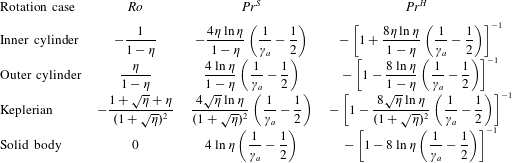
of the realistic Taylor–Couette cell, see table 1 containing the four different rotation cases: sole rotation of the inner cylinder (
 $\unicode[STIX]{x1D707}=0$
), Keplerian rotation (
 $\unicode[STIX]{x1D707}=\unicode[STIX]{x1D702}^{3/2}$
), sole rotation of the outer cylinder (
 $\unicode[STIX]{x1D707}\rightarrow \infty$
), and solid body rotation
 $(\unicode[STIX]{x1D707}=1)$
. In particular,
 $Rt<0$
for the Taylor–Couette system due to the geometric constraint
 $0<\unicode[STIX]{x1D702}<1$
and the temperature variation is such that
 $0\leqslant \hat{\unicode[STIX]{x1D6E9}}\leqslant 1$
.
5 Local instabilities
5.1 Diffusionless instabilities
In the case when the viscosity and thermal diffusivity are both set to zero in (4.6) or, equivalently,
 $Ta\rightarrow \infty$
in (4.9), the dispersion relation (4.11) factorizes to
 $$\begin{eqnarray}\unicode[STIX]{x1D712}(\unicode[STIX]{x1D712}^{2}+4(1+Ro)(1-\unicode[STIX]{x1D6FE}_{a}\hat{\unicode[STIX]{x1D6E9}})-2\unicode[STIX]{x1D6FE}_{a}\hat{\unicode[STIX]{x1D6E9}}Rt)=0.\end{eqnarray}$$
The root
 $\unicode[STIX]{x1D712}=0$
corresponds to the pure imaginary eigenvalue
 $\unicode[STIX]{x1D706}=\unicode[STIX]{x1D6FD}\unicode[STIX]{x1D6FA}s=-\text{i}m\unicode[STIX]{x1D6FA}$
describing a stable rotating wave with the local frequency
 $\unicode[STIX]{x1D6FA}$
. Similarly, the flow admits stable inertial waves with frequencies given by
 $$\begin{eqnarray}\frac{\unicode[STIX]{x1D714}}{\unicode[STIX]{x1D6FA}}=-m\pm \unicode[STIX]{x1D6FD}\sqrt{4(1+Ro)(1-\unicode[STIX]{x1D6FE}_{a}\hat{\unicode[STIX]{x1D6E9}})-2\unicode[STIX]{x1D6FE}_{a}\hat{\unicode[STIX]{x1D6E9}}Rt},\end{eqnarray}$$
if the radicand in (5.2) is positive:
 $$\begin{eqnarray}4(1+Ro)(1-\unicode[STIX]{x1D6FE}_{a}\hat{\unicode[STIX]{x1D6E9}})-2\unicode[STIX]{x1D6FE}_{a}\hat{\unicode[STIX]{x1D6E9}}Rt>0.\end{eqnarray}$$
These inertial waves result from the combined effects of the rotation and the temperature gradient. While the term
 $\unicode[STIX]{x1D6FE}_{a}\hat{\unicode[STIX]{x1D6E9}}$
is very weak in the Boussinesq approximation, the term
 $\unicode[STIX]{x1D6FE}_{a}\hat{\unicode[STIX]{x1D6E9}}Rt$
can become significant depending on the steepness of the temperature profile. In the isothermal case (
 $\unicode[STIX]{x1D6FE}_{a}=0$
), we retrieve the frequency of the Kelvin waves in rotating flows.
The inequality (5.3) contains the generalized Rayleigh criterion derived in Mutabazi & Bahloul (Reference Mutabazi and Bahloul2002) and Meyer et al. (Reference Meyer, Yoshikawa and Mutabazi2015) for the stability of inviscid flow with curved streamlines and a radial temperature gradient. Indeed, Mutabazi & Bahloul (Reference Mutabazi and Bahloul2002) and Meyer et al. (Reference Meyer, Yoshikawa and Mutabazi2015) found the criterion for stability against axisymmetric perturbations in the diffusionless case in terms of the generalized Rayleigh discriminant
 $\unicode[STIX]{x1D6F9}(r)$
:
 $$\begin{eqnarray}\unicode[STIX]{x1D6F9}(r)>0,\quad \unicode[STIX]{x1D6F9}(r)=\unicode[STIX]{x1D6F7}-\unicode[STIX]{x1D6FE}_{a}\left(\hat{\unicode[STIX]{x1D6E9}}\unicode[STIX]{x1D6F7}+\frac{\text{d}\hat{\unicode[STIX]{x1D6E9}}}{\text{d}r}\frac{V^{2}}{r}\right),\quad \unicode[STIX]{x1D6F7}(r)=\frac{1}{r^{3}}\frac{\text{d}(rV)^{2}}{\text{d}r}.\end{eqnarray}$$
Expressing the classical hydrodynamic Rayleigh discriminant
 $\unicode[STIX]{x1D6F7}(r)$
via the hydrodynamic Rossby number as
 $\unicode[STIX]{x1D6F7}=4\unicode[STIX]{x1D6FA}^{2}(1+Ro)$
, we obtain
 $$\begin{eqnarray}\unicode[STIX]{x1D6F9}=\unicode[STIX]{x1D6FA}^{2}\{4(1+Ro)-2\unicode[STIX]{x1D6FE}_{a}\hat{\unicode[STIX]{x1D6E9}}[Rt+2(1+Ro)]\}.\end{eqnarray}$$
Requiring
 $\unicode[STIX]{x1D6F9}>0$
we arrive exactly at the criterion (5.3). The opposite inequality
 $\unicode[STIX]{x1D6F9}<0$
or
 $4(1+Ro)(1-\unicode[STIX]{x1D6FE}_{a}\hat{\unicode[STIX]{x1D6E9}})-2\unicode[STIX]{x1D6FE}_{a}\hat{\unicode[STIX]{x1D6E9}}Rt<0$
coincides with the condition for instability to stationary axisymmetric perturbations known as the diffusionless Goldreich–Schubert–Fricke (GSF) instability (Acheson & Gibbons Reference Acheson and Gibbons1978).
5.2 Enhancement of stability by viscosity and thermal diffusivity at
 $Pr=1$

In the case when
 $Pr=1$
(i.e. when the viscous and thermal diffusion timescales are equal) the dispersion relation (4.11) can also be factorized:
 $$\begin{eqnarray}\left(\unicode[STIX]{x1D712}+\frac{1}{Ta}\right)\left[\left(\unicode[STIX]{x1D712}+\frac{1}{Ta}\right)^{2}+4(1-\unicode[STIX]{x1D6FE}_{a}\hat{\unicode[STIX]{x1D6E9}})(1+Ro)-2\unicode[STIX]{x1D6FE}_{a}\hat{\unicode[STIX]{x1D6E9}}Rt\right]=0.\end{eqnarray}$$
By this reasoning, the roots of the dispersion relation (5.6) can be found explicitly:
 $$\begin{eqnarray}\displaystyle & \displaystyle s_{1,2}=-\frac{1}{Ta}-\text{i}n\pm \text{i}\sqrt{4(1+Ro)(1-\unicode[STIX]{x1D6FE}_{a}\hat{\unicode[STIX]{x1D6E9}})-2\unicode[STIX]{x1D6FE}_{a}\hat{\unicode[STIX]{x1D6E9}}Rt}, & \displaystyle\end{eqnarray}$$
 $$\begin{eqnarray}\displaystyle & \displaystyle s_{3}=-\frac{1}{Ta}-\text{i}n. & \displaystyle\end{eqnarray}$$
The mode with the eigenvalue
 $s_{3}$
is a pure hydrodynamic mode as it does not contain the temperature gradient, it is damped by the viscosity. The modes corresponding to the eigenvalue
 $s_{1,2}$
contain both the hydrodynamic and thermal effects. One of the modes is always damped, the other one should be excited when its growth rate vanishes, i.e. when
 $$\begin{eqnarray}4(1+Ro)(1-\unicode[STIX]{x1D6FE}_{a}\hat{\unicode[STIX]{x1D6E9}})-2\unicode[STIX]{x1D6FE}_{a}\hat{\unicode[STIX]{x1D6E9}}Rt+\frac{1}{Ta^{2}}=0.\end{eqnarray}$$
The double-diffusive stability criterion given by the requirement for the left-hand side of (5.9) to be positive suggests that at
 $Pr=1$
the viscosity and thermal diffusivity enlarge the stability domain of the diffusionless system. Furthermore, in the limit
 $Ta\rightarrow \infty$
the roots (5.7) and (5.8) reduce to the roots of the diffusionless dispersion relation (5.1), whereas the double-diffusive stability criterion reduces to the diffusionless criterion (5.3).
Note that the limiting procedure that first makes the diffusion coefficients of a dissipative system with two diffusion mechanisms equal and then tends them to zero typically yields a correct diffusionless stability criterion in many double-diffusive systems of hydrodynamics and magnetohydrodynamics (Kirillov et al. Reference Kirillov, Stefani and Fukumoto2014; Kirillov Reference Kirillov2016). In general, the limit of zero dissipation of the double-diffusive stability criteria should not necessarily coincide with the diffusionless stability criteria (Acheson & Gibbons Reference Acheson and Gibbons1978; Kirillov & Verhulst Reference Kirillov and Verhulst2010; Kirillov Reference Kirillov2013).
5.3 Double-diffusive flow stability criteria at arbitrary
$Pr$

We derive stability conditions of the base flow at arbitrary
 $Pr$
by applying the Lienard–Chipart stability criterion (Kirillov Reference Kirillov2013) to the real polynomial (4.11) of degree 3 in
 $\unicode[STIX]{x1D712}$
:
 $$\begin{eqnarray}a_{0}>0,\quad a_{2}>0,\quad -a_{0}(a_{0}-a_{1}a_{2})>0.\end{eqnarray}$$
The second inequality is always fulfilled whereas the first one yields:
 $$\begin{eqnarray}4(1+Ro)(1-\unicode[STIX]{x1D6FE}_{a}\hat{\unicode[STIX]{x1D6E9}})-2\unicode[STIX]{x1D6FE}_{a}\hat{\unicode[STIX]{x1D6E9}}RtPr+\frac{1}{Ta^{2}}>0.\end{eqnarray}$$
The condition (5.11) is a modified Rayleigh criterion that takes into account both the kinematic viscosity and the thermal diffusion. Writing it as
 $$\begin{eqnarray}\displaystyle 1+Ro>\frac{2\unicode[STIX]{x1D6FE}_{a}\hat{\unicode[STIX]{x1D6E9}}\,RtPr}{4(1-\unicode[STIX]{x1D6FE}_{a}\hat{\unicode[STIX]{x1D6E9}})}-\frac{1}{4Ta^{2}(1-\unicode[STIX]{x1D6FE}_{a}\hat{\unicode[STIX]{x1D6E9}})}, & & \displaystyle\end{eqnarray}$$
we conclude that, for
 $Rt<0$
and
 $0\leqslant \hat{\unicode[STIX]{x1D6E9}}\leqslant 1$
, the kinematic viscosity and outward heating
 $(\unicode[STIX]{x1D6FE}_{a}>0)$
are stabilizing and inward heating
 $(\unicode[STIX]{x1D6FE}_{a}<0)$
is destabilizing with respect to the Rayleigh criterion (
 $1+Ro>0$
) for an ideal incompressible fluid.
At
 $Pr=1$
the condition (5.11) reduces to the criterion (5.9). Furthermore, the limit
 $Ta\rightarrow \infty$
applied to (5.11) yields the diffusionless criterion (5.3) only if
 $Pr=1$
.
The condition
 $a_{0}=0$
yields the control parameter
 $Ta$
as a function of the other control parameters:
 $$\begin{eqnarray}Ta_{c}^{S}=\frac{1}{\sqrt{2\unicode[STIX]{x1D6FE}_{a}\hat{\unicode[STIX]{x1D6E9}}RtPr-4(1+Ro)(1-\unicode[STIX]{x1D6FE}_{a}\hat{\unicode[STIX]{x1D6E9}})}}.\end{eqnarray}$$
Since at
 $a_{0}=0$
the dispersion equation (4.11) has the root
 $\unicode[STIX]{x1D712}=0$
, corresponding to
 $s=-\text{i}n$
, the relation (5.13) is the threshold of the double-diffusive Goldreich–Schubert–Fricke instability (Acheson & Gibbons Reference Acheson and Gibbons1978), which is a stationary axisymmetric instability in the case when
 $n=0$
.
The third inequality of (5.10) yields
 $$\begin{eqnarray}\displaystyle -\left(\unicode[STIX]{x1D6FE}_{a}\hat{\unicode[STIX]{x1D6E9}}(Pr+1)Rt-4Pr(1-\unicode[STIX]{x1D6FE}_{a}\hat{\unicode[STIX]{x1D6E9}})(1+Ro)-\frac{(Pr+1)^{2}}{PrTa^{2}}\right)>0, & & \displaystyle\end{eqnarray}$$
from which the threshold of the oscillatory instability through a Hopf bifurcation naturally follows:
 $$\begin{eqnarray}Ta_{c}^{H}=\frac{Pr+1}{\sqrt{Pr(Pr+1)\unicode[STIX]{x1D6FE}_{a}\hat{\unicode[STIX]{x1D6E9}}Rt-4Pr^{2}(1-\unicode[STIX]{x1D6FE}_{a}\hat{\unicode[STIX]{x1D6E9}})(1+Ro)}}.\end{eqnarray}$$
Indeed, from the Vieta’s formulas (Vinberg Reference Vinberg2003)
 $$\begin{eqnarray}\unicode[STIX]{x1D712}_{1}+\unicode[STIX]{x1D712}_{2}+\unicode[STIX]{x1D712}_{3}=-a_{2},\quad \unicode[STIX]{x1D712}_{1}\unicode[STIX]{x1D712}_{2}+\unicode[STIX]{x1D712}_{2}\unicode[STIX]{x1D712}_{3}+\unicode[STIX]{x1D712}_{3}\unicode[STIX]{x1D712}_{1}=a_{1},\quad \unicode[STIX]{x1D712}_{1}\unicode[STIX]{x1D712}_{2}\unicode[STIX]{x1D712}_{3}=-a_{0}\end{eqnarray}$$
it follows that at
 $Ta=Ta_{c}^{H}$
the characteristic equation (4.11) admits two imaginary roots
 $\unicode[STIX]{x1D712}_{1,2}=\pm \text{i}\bar{\unicode[STIX]{x1D714}}_{c}$
, corresponding to
 $s=-\text{i}n\pm \text{i}\bar{\unicode[STIX]{x1D714}}_{c}$
, where
 $n$
can be either zero or not, and one real root
 $\unicode[STIX]{x1D712}_{3}=-a_{2}$
. The real root corresponds to a damped mode while the imaginary roots yield the Hopf frequency
 $\bar{\unicode[STIX]{x1D714}}_{c}$
given by
 $$\begin{eqnarray}\bar{\unicode[STIX]{x1D714}}_{c}=\frac{\sqrt{4(1+Ro)(1-\unicode[STIX]{x1D6FE}_{a}\hat{\unicode[STIX]{x1D6E9}})-\unicode[STIX]{x1D6FE}_{a}\hat{\unicode[STIX]{x1D6E9}}RtPr(Pr+1)}}{Pr+1}\end{eqnarray}$$
and describe a marginal oscillatory mode. The total frequency of this marginal mode is given by
 $\unicode[STIX]{x1D714}_{c}=-\unicode[STIX]{x1D6FD}\unicode[STIX]{x1D6FA}(n\pm \bar{\unicode[STIX]{x1D714}}_{c})$
. The marginal value
 $Ta_{c}^{H}$
corresponds to a Hopf bifurcation of the base flow to a state oscillating with a Hopf frequency
 $\bar{\unicode[STIX]{x1D714}}_{c}$
. For
 $n=0$
, the marginal mode is an oscillatory axisymmetric mode, while for
 $n\neq 0$
, the marginal mode is an oscillatory non-axisymmetric mode.
5.4 Codimension-2 points in the case of the Rayleigh-unstable flows
In the parameter space, the boundary of the stationary instability (5.13), corresponding to a simple zero root, and the boundary of the Hopf bifurcation (5.15), corresponding to a pair of imaginary roots, may have common codimension-2 points with the coordinates
 $(Pr^{\ast },Ta^{\ast })$
given for
 $Ro+1<0$
and
 $\unicode[STIX]{x1D6FE}_{a}>0$
by
 $$\begin{eqnarray}\displaystyle & \displaystyle Pr^{\ast }=-\frac{1}{2}+\frac{1}{2}\sqrt{1+16\frac{(1-\unicode[STIX]{x1D6FE}_{a}\hat{\unicode[STIX]{x1D6E9}})}{\unicode[STIX]{x1D6FE}_{a}\hat{\unicode[STIX]{x1D6E9}}}\frac{(1+Ro)}{Rt}}, & \displaystyle\end{eqnarray}$$
 $$\begin{eqnarray}\displaystyle & \displaystyle Ta^{\ast }=\frac{1}{\sqrt{2\unicode[STIX]{x1D6FE}_{a}\hat{\unicode[STIX]{x1D6E9}}RtPr^{\ast }-4(1-\unicode[STIX]{x1D6FE}_{a}\hat{\unicode[STIX]{x1D6E9}})(1+Ro)}}. & \displaystyle\end{eqnarray}$$
5.5 The Rayleigh line
In the particular case
 $Ro=-1$
, corresponding to the Rayleigh line, the roots of the dispersion relation are found explicitly for an arbitrary
 $Pr$
:
 $$\begin{eqnarray}\displaystyle \unicode[STIX]{x1D712}_{1,2}=-\frac{Pr+1}{2TaPr}\pm \sqrt{2Rt\hat{\unicode[STIX]{x1D6E9}}\unicode[STIX]{x1D6FE}_{a}+\frac{(Pr-1)^{2}}{4Ta^{2}Pr^{2}}},\quad \unicode[STIX]{x1D712}_{3}=-\frac{1}{Ta}. & & \displaystyle\end{eqnarray}$$
One of the first two roots vanishes at the threshold of stationary instability
 $Ta=Ta_{c}^{S}$
, where
 $(\unicode[STIX]{x1D6FE}_{a}<0,Rt<0)$
 $$\begin{eqnarray}\displaystyle Ta_{c}^{S}=\frac{1}{\sqrt{2\unicode[STIX]{x1D6FE}_{a}\hat{\unicode[STIX]{x1D6E9}}RtPr}}. & & \displaystyle\end{eqnarray}$$
Thus, at the Rayleigh line, stationary instability is possible for inward heating only. When the heating is outward and
 $Rt<0$
, both the criteria (5.11) and (5.14) are fulfilled and the flow is stable.
6 Stationary and oscillatory modes
The relations (5.13) and (5.15) contain, besides
 $Pr$
, the group of parameters
 $Ro$
,
 $\unicode[STIX]{x1D6FE}_{a}\hat{\unicode[STIX]{x1D6E9}}$
and
 $\unicode[STIX]{x1D6FE}_{a}\hat{\unicode[STIX]{x1D6E9}}Rt$
,
 $Rt<0$
. Therefore, the conditions for the occurrence of stationary or oscillatory modes can be analysed in terms of these parameters.
Let us define the Brunt–Väisälä frequency
 $N$
as Meyer et al. (Reference Meyer, Yoshikawa and Mutabazi2015) (these authors have defined
 $N^{2}$
with the opposite sign)
 $$\begin{eqnarray}\displaystyle N^{2}=\frac{1}{\unicode[STIX]{x1D70C}_{0}}\unicode[STIX]{x1D735}\unicode[STIX]{x1D70C}\boldsymbol{\cdot }\boldsymbol{g}_{cB}=\frac{1}{\unicode[STIX]{x1D70C}_{0}}\frac{\text{d}\unicode[STIX]{x1D70C}}{\text{d}r}\frac{V^{2}}{r}. & & \displaystyle\end{eqnarray}$$
Taking into account that
 $\unicode[STIX]{x1D70C}(r)=\unicode[STIX]{x1D70C}_{0}(1-\unicode[STIX]{x1D6FC}\unicode[STIX]{x1D703}(r))$
in the Boussinesq approximation, we conclude that
 $N^{2}=-2\unicode[STIX]{x1D6FE}_{a}\hat{\unicode[STIX]{x1D6E9}}Rt\,\unicode[STIX]{x1D6FA}^{2}$
.
In the diffusionless case, for
 $Ro<-1$
, the flow is Rayleigh unstable, i.e. the radial stratification of the square of the angular momentum is negative; for
 $Ro>-1$
, the flow is Rayleigh stable (Chandrasekhar Reference Chandrasekhar1961). The centrifugal acceleration is oriented away from the rotation axis, implying that outward heating (
 $\unicode[STIX]{x1D6FE}_{a}>0$
) corresponds to a stable stratification of the density (
 $N^{2}>0$
) while inward heating (
 $\unicode[STIX]{x1D6FE}_{a}<0$
) corresponds to an unstable density stratification, characterized by the negative sign of the squared Brunt–Väisälä frequency
 $(N^{2}<0)$
.
For Rayleigh-stable flow configurations, negative stratification of the density yields a thermal instability analogue to Rayleigh–Bénard convection, which might lead to stationary modes at the onset. For Rayleigh-unstable configurations, negative density stratification enforces the centrifugal instability and decreases the threshold compared to the isothermal flow; while positive density stratification will delay the threshold and inertial waves may be excited by the rotation when
 $N^{2}$
becomes significant. These inertial waves, observed in numerical simulations, have been recently reported in Meyer et al. (Reference Meyer, Yoshikawa and Mutabazi2015).
6.1 Stationary modes
Taking into account the relations (4.16) we write the threshold for the onset of stationary instability (5.13) in terms of the parameters of Couette–Taylor flow
 $$\begin{eqnarray}r_{S}=\frac{Ta_{c}^{S}}{Ta_{0}}=\left[1-\frac{\unicode[STIX]{x1D6FE}_{a}}{2}+\frac{\unicode[STIX]{x1D6FE}_{a}Pr}{\ln \unicode[STIX]{x1D702}}\left(Ta_{0}\right)^{2}\right]^{-1/2},\end{eqnarray}$$
where we have introduced the threshold for the isothermal flow as follows
 $$\begin{eqnarray}Ta_{c}^{S}(\unicode[STIX]{x1D6FE}_{a}=0)=\frac{1}{2}\sqrt{\frac{-1}{Ro+1}}\equiv Ta_{0}.\end{eqnarray}$$
For circular Couette flow, the quantity
 $(Ta_{0})^{2}$
is positive when
 $Ro+1<0$
(or
 $\unicode[STIX]{x1D707}<\unicode[STIX]{x1D702}^{2}$
), i.e. in the Rayleigh-unstable zone, and
 $(Ta_{0})^{2}<0$
when
 $Ro+1>0$
, i.e. in the Rayleigh-stable zone (Chandrasekhar Reference Chandrasekhar1961). The explicit expressions for
 $Ta_{c}^{S}$
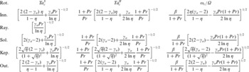
calculated for different rotating regimes of Couette–Taylor flow are given in table 2.
Thresholds of the critical modes and the critical Hopf frequency for different rotation regimes in the Couette–Taylor system: (Inn.) inner cylinder rotating, (Ray.) Rayleigh line, (Sol.) solid body rotation, (Kep.) Keplerian rotation, (Out.) outer cylinder rotating.

Rotating inner cylinder with
 $\unicode[STIX]{x1D707}=0$
,
 $\unicode[STIX]{x1D702}=0.99$
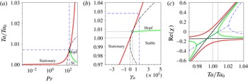
. (a) Stability diagram at
 $\unicode[STIX]{x1D6FE}_{a}=0.0004$
showing the boundaries of stationary instability (6.2) and Hopf bifurcation (6.6) that have a common codimension-2 point
 $(Pr^{\ast }\approx 140.55,Ta^{\ast }/Ta_{0}\approx 1.0072)$
given by (6.8) and (6.9). The black dashed line corresponds to double real roots
 $\unicode[STIX]{x1D712}$
:
 $\unicode[STIX]{x1D712}<0$
in the stability domain,
 $\unicode[STIX]{x1D712}>0$
in the instability domain, and
 $\unicode[STIX]{x1D712}=0$
at the codimension-2 point. (b) The critical values of
 $Ta/Ta_{0}$
versus
 $\unicode[STIX]{x1D6FE}_{a}$
at
 $Pr\approx 140.55$
with the codimension-2 point
 $(\unicode[STIX]{x1D6FE}_{a}=0.0004,Ta/Ta_{0}\approx 1.0072)$
and the (black dashed) line of real eigenvalues. (c) Growth rates (
 $\text{Re}\unicode[STIX]{x1D712}$
) at
 $Pr\approx 140.55$
and (red)
 $\unicode[STIX]{x1D6FE}_{a}=-0.0004$
, (black)
 $\unicode[STIX]{x1D6FE}_{a}=0$
, (green)
 $\unicode[STIX]{x1D6FE}_{a}=0.0004$
, (dashdot blue)
 $\unicode[STIX]{x1D6FE}_{a}=0.0015$
.

In figure 1 we plot the threshold (6.2) in the Rayleigh-unstable case of the inner cylinder rotation with
 $\unicode[STIX]{x1D707}=0$
and
 $Ro+1=-\unicode[STIX]{x1D702}/(1-\unicode[STIX]{x1D702})<0$
, see table 1. We see that the ratio
 $r_{S}<1$
, i.e. there is a destabilization, for inward heating
 $(\unicode[STIX]{x1D6FE}_{a}<0)$
, and
 $r_{S}>1$
for outward heating
 $(\unicode[STIX]{x1D6FE}_{a}>0)$
. Note that the threshold of the stationary modes (6.2) is a function of the parameter
 $\widehat{S}=-\unicode[STIX]{x1D6FE}_{a}Pr/\ln \unicode[STIX]{x1D702}$
, where
 $|\unicode[STIX]{x1D6FE}_{a}|\ll 1$
in the Boussinesq approximation. This result theoretically justifies the numerical analysis of Meyer et al. (Reference Meyer, Yoshikawa and Mutabazi2015), where it was shown that the stationary critical modes almost scaled with the temperature drop coefficient
 $S=\widehat{S}\unicode[STIX]{x1D702}/(1-\unicode[STIX]{x1D702})$
.
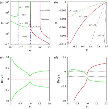
Keplerian case with
 $\unicode[STIX]{x1D707}=\unicode[STIX]{x1D702}^{3/2}$
and
 $\unicode[STIX]{x1D702}=0.99$
. (a) Variation of the threshold of the stationary instability and Hopf bifurcation with
 $Pr$
at
 $\unicode[STIX]{x1D6FE}_{a}<0$
(an inward temperature gradient). The asymptotic values of
 $Pr$
marked by dot-dashed lines are, respectively:
 $Pr^{H}\approx 0.0523$
,
 $Pr^{H}\approx 0.98$
,
 $Pr^{S}\approx 1.01$
and
 $Pr^{S}\approx 10.055$
. (b) Lines
 $Pr^{S}=\text{const.}$
in the
 $(\unicode[STIX]{x1D702},\unicode[STIX]{x1D6FE}_{a})$
-plane. (c,d) Variation of the frequencies
 $\text{Im}(\unicode[STIX]{x1D712})$
and the growth rates
 $\text{Re}(\unicode[STIX]{x1D712})$
with
 $Pr$
at
 $Ta=6$
and
 $\unicode[STIX]{x1D6FE}_{a}=-0.01$
(an inward temperature gradient). The green lines correspond to oscillatory modes, and the red lines to stationary modes.

Stationary modes can exist if the radicand in (5.13) is positive, this yields a condition on
 $Pr$
to be satisfied. In the case of Rayleigh-unstable flow, i.e. when
 $1+Ro<0$
, the stationary modes exist for any value of
 $Pr$
when
 $\unicode[STIX]{x1D6FE}_{a}<0$
and for
 $0\leqslant Pr<Pr^{S}$
when
 $\unicode[STIX]{x1D6FE}_{a}>0$
, where the critical value of the Prandtl number is
 $$\begin{eqnarray}Pr^{S}=\frac{2(1+Ro)(1-\unicode[STIX]{x1D6FE}_{a}\hat{\unicode[STIX]{x1D6E9}})}{\unicode[STIX]{x1D6FE}_{a}\hat{\unicode[STIX]{x1D6E9}}Rt}.\end{eqnarray}$$
The values of
 $Pr^{S}$
calculated in terms of the parameters (4.16) for different rotating cases of the Couette–Taylor system are given in table 1. In the case of the rotating inner cylinder shown in figure 1(a) the asymptotic value (6.4) for the threshold (6.2) is
 $Pr^{S}\approx 9948$
.
(a) Solid body rotation with
 $\unicode[STIX]{x1D707}=1$
and
 $\unicode[STIX]{x1D702}=0.99$
. Thresholds of the stationary instability and Hopf bifurcation with the asymptotic values of
 $Pr$
marked by dot-dashed lines:
 $Pr^{H}\approx 0.0126$
,
 $Pr^{H}\approx 0.1412$
,
 $Pr^{S}\approx 4.0402$
, and
 $Pr^{S}\approx 40.221$
. (b) Outer cylinder rotation with
 $\unicode[STIX]{x1D707}=\infty$
and
 $\unicode[STIX]{x1D702}=0.99$
. Thresholds of the stationary instability and Hopf bifurcation with the asymptotic values of the Prandtl number:
 $Pr^{H}\approx 0.0012$
and
 $Pr^{S}\approx 404.02$
. (c,d) Variation of the (c) frequencies and (d) growth rates with
 $Pr$
for outer cylinder rotation (
 $\unicode[STIX]{x1D707}=\infty$
,
 $\unicode[STIX]{x1D702}=0.99$
) at given
 $Ta=1000$
and
 $\unicode[STIX]{x1D6FE}_{a}=-0.01$
. The green lines correspond to the oscillatory modes and the red line corresponds to a (damped) stationary mode.

In the case of Rayleigh-stable flows
 $(1+Ro>0)$
, the stationary modes are expected only for inward heating (
 $\unicode[STIX]{x1D6FE}_{a}<0$
) at
 $Pr>Pr^{S}$
. Figure 2 shows the variation of the threshold with
 $Pr$
for Keplerian rotation in the small gap case
 $\unicode[STIX]{x1D702}=0.99$
; the corresponding stability diagrams for the cases of solid body rotation and outer cylinder rotation are shown in figure 3.
Note that for the Rayleigh-unstable flows the stationary modes exist even in the limit of vanishing Prandtl number (
 $Pr\rightarrow 0$
), i.e. for highly thermally conducting liquids with low kinematic viscosity. In this limit, the threshold (5.13) reduces to the expression
 $$\begin{eqnarray}Ta_{c}^{S}=\frac{1}{\sqrt{-4(1+Ro)(1-\unicode[STIX]{x1D6FE}_{a}\hat{\unicode[STIX]{x1D6E9}})}}.\end{eqnarray}$$
For Rayleigh-stable flows
 $(1+Ro>0)$
the threshold of the stationary modes (5.13) decreases towards zero at
 $\unicode[STIX]{x1D6FE}_{a}<0$
in the limit of large values of the Prandtl number (
 $Pr\rightarrow \infty$
), i.e. for highly viscous and poorly heat-conducting fluids, see figures 2 and 3.
6.2 Hopf bifurcation
In terms of the parameters (4.16) and (6.3) the threshold for the onset of oscillatory instability (5.15) becomes
 $$\begin{eqnarray}\displaystyle r_{H}=\frac{Ta_{c}^{H}}{Ta_{0}}=\frac{Pr+1}{Pr}\left[1-\frac{\unicode[STIX]{x1D6FE}_{a}}{2}+\frac{\unicode[STIX]{x1D6FE}_{a}}{2\ln \unicode[STIX]{x1D702}}\frac{Pr+1}{Pr}\left(Ta_{0}\right)^{2}\right]^{-1/2} & & \displaystyle\end{eqnarray}$$
and the Hopf frequency of the oscillatory modes (5.17) acquires the form
 $$\begin{eqnarray}\frac{\unicode[STIX]{x1D714}_{c}}{\unicode[STIX]{x1D6FA}}=\frac{\unicode[STIX]{x1D6FD}}{Pr+1}\frac{1}{Ta_{0}}\sqrt{-1+\frac{\unicode[STIX]{x1D6FE}_{a}}{2}-\frac{\unicode[STIX]{x1D6FE}_{a}Pr(Pr+1)}{2\ln \unicode[STIX]{x1D702}}\left(Ta_{0}\right)^{2}}.\end{eqnarray}$$
Rotating inner cylinder with
 $\unicode[STIX]{x1D707}=0$
and
 $\unicode[STIX]{x1D702}=0.99$
. The critical frequency
 $\unicode[STIX]{x1D714}_{c}$
at the onset of (red) stationary instability and (green) Hopf bifurcation in units of
 $\unicode[STIX]{x1D6FD}\unicode[STIX]{x1D6FA}$
(a) versus
 $Pr$
at
 $\unicode[STIX]{x1D6FE}_{a}=0.0004$
and (b) versus
 $\unicode[STIX]{x1D6FE}_{a}$
according to (6.7). The limiting frequency (6.12) at
 $\unicode[STIX]{x1D6FE}_{a}=0.0004$
is
 $(\unicode[STIX]{x1D714}_{\infty }/\unicode[STIX]{x1D6FD}\unicode[STIX]{x1D6FA})\approx 0.1411$
. (c) The critical Hopf frequency
 $\unicode[STIX]{x1D714}_{c}$
as a function of the Brunt–Väisälä frequency
 $N$
according to (6.11) and (6.13). The critical frequency vanishes at
 $N_{c}/\unicode[STIX]{x1D6FA}\approx 0.5572$
for
 $Pr=50$
, at
 $N_{c}/\unicode[STIX]{x1D6FA}\approx 0.28$
for
 $Pr=100$
, and at
 $N_{c}/\unicode[STIX]{x1D6FA}\approx 0.0281$
for
 $Pr=1000$
calculated by means of (6.14) and (4.16).

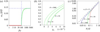
Figure 1(a,b) illustrates the variation of the threshold of Hopf bifurcation with
 $Pr$
and
 $\unicode[STIX]{x1D6FE}_{a}$
for circular Couette flow with the inner cylinder rotating alone. The variation of the Hopf frequency with
 $Pr$
and
 $\unicode[STIX]{x1D6FE}_{a}$
in this rotating case is shown in figure 4. Similarly to stationary instability, both the threshold (6.6) and the frequency (6.7) of the oscillatory modes depend explicitly on the Prandtl number
 $Pr$
and on the temperature drop parameter
 $\widehat{S}$
, in agreement with the numerical calculations of (Meyer et al.
Reference Meyer, Yoshikawa and Mutabazi2015).
We see that at
 $\unicode[STIX]{x1D6FE}_{a}>0$
both
 $r_{H}>1$
and
 $r_{S}>1$
, i.e. outward heating is stabilizing for both stationary and oscillatory modes with respect to isothermal flow. The growth rates shown in figure 1(c) demonstrate that the complex roots do not exist at
 $\unicode[STIX]{x1D6FE}_{a}\leqslant 0$
; they appear at
 $\unicode[STIX]{x1D6FE}_{a}>0$
due to splitting of a double real eigenvalue. When this eigenvalue is negative the complex roots are stable. They acquire a positive growth rate only after a double real eigenvalue passes through zero with the change of parameters, which happens exactly at a codimension-2 point, cf. Tuckerman (Reference Tuckerman2001).
Indeed, since this flow is Rayleigh-unstable in the absence of diffusion, the branches of the stationary and oscillatory modes have a common codimension-2 point with the coordinates (5.18) and (5.19) that in the parametric representation, (4.16) and (6.3) can be written as follows:
 $$\begin{eqnarray}\displaystyle & \displaystyle Pr^{\ast }=-\frac{1}{2}+\frac{1}{2}\sqrt{1-4\frac{2-\unicode[STIX]{x1D6FE}_{a}}{\unicode[STIX]{x1D6FE}_{a}}\frac{\ln \unicode[STIX]{x1D702}}{(Ta_{0})^{2}}}, & \displaystyle\end{eqnarray}$$
 $$\begin{eqnarray}\displaystyle & \displaystyle Ta^{\ast }=Ta_{0}\left[1-\frac{\unicode[STIX]{x1D6FE}_{a}}{2}+\unicode[STIX]{x1D6FE}_{a}Pr^{\ast }\frac{\left(Ta_{0}\right)^{2}}{\ln \unicode[STIX]{x1D702}}\right]^{-1/2}. & \displaystyle\end{eqnarray}$$
At the codimension-2 point one of the roots of the dispersion relation is double zero and the other one is simple real and negative, corresponding to a damped mode, as the growth rates demonstrate in figure 1(c).
The threshold for the excitation of oscillatory modes and the corresponding critical frequency of the oscillatory modes for both the Rayleigh-stable and the Rayleigh-unstable rotation regimes in the Couette–Taylor system are summarized in table 2. For the Rayleigh-unstable flows with outward heating the oscillatory instability actually occurs at
 $Pr>Pr^{\ast }$
, where
 $Pr^{\ast }$
is given by (5.18) or (6.8), see figure 1.
Figures 2 and 3 show the boundaries of stationary instability and Hopf bifurcation in the
 $(Pr,Ta)$
-plane for Rayleigh-stable flows such as Keplerian rotation, solid-body rotation and the case of the outer cylinder rotating. We see also that the frequency of the oscillatory instability is increasing while approaching the outer cylinder rotating case, whereas the growth rate of the oscillatory instability at low
 $Pr$
is decreasing.
All these Rayleigh-stable flows (
 $1+Ro>0$
or
 $\unicode[STIX]{x1D707}\geqslant \unicode[STIX]{x1D702}^{2}$
) with inward heating
 $(\unicode[STIX]{x1D6FE}_{a}<0)$
share the same property. Namely, the oscillatory modes are excited when thermal diffusion dominates over the fluid viscosity
 $$\begin{eqnarray}0<Pr<Pr^{H}=\frac{\unicode[STIX]{x1D6FE}_{a}\hat{\unicode[STIX]{x1D6E9}}Rt}{\unicode[STIX]{x1D6FE}_{a}\hat{\unicode[STIX]{x1D6E9}}Rt-4(1+Ro)(1-\unicode[STIX]{x1D6FE}_{a}\hat{\unicode[STIX]{x1D6E9}})}<1.\end{eqnarray}$$
This result follows from the observation that the Hopf bifurcation from the base flow can occur if the radicand in (5.15) is positive. In contrast, the stationary modes are excited in the Rayleigh-stable flow by inward heating when
 $Pr>Pr^{S}>1$
, where
 $Pr^{S}$
is given in (6.4) and table 1.
Therefore, for Rayleigh-stable flows an inward radial temperature gradient destabilizes the flow depending on the value of
 $Pr$
. The oscillatory instability occurs at
 $0<Pr<1$
while the stationary instability takes place at
 $Pr>1$
. At
 $Pr=1$
the flows remain stable, becoming unstable only when
 $Pr\neq 1$
, which is a characteristic feature of double-diffusive instabilities (Acheson & Gibbons Reference Acheson and Gibbons1978; Kirillov & Verhulst Reference Kirillov and Verhulst2010; Kirillov Reference Kirillov2013).
As figures 2 and 3 demonstrate, when
 $Pr\rightarrow 0$
, the threshold of the oscillatory modes (5.15) occurring in the Rayleigh-stable flows becomes infinite
 $(Ta_{c}^{H}\rightarrow \infty )$
while their frequency
 $\bar{\unicode[STIX]{x1D714}}_{c}\rightarrow 2\sqrt{(1+Ro)(1-\unicode[STIX]{x1D6FE}_{a}\hat{\unicode[STIX]{x1D6E9}})}$
depends weakly on the heating parameter
 $\unicode[STIX]{x1D6FE}_{a}$
.
The opposite limit, when
 $Pr\rightarrow \infty$
, is applicable to the threshold of Hopf bifurcation in Rayleigh-unstable flows with outward heating
 $(\unicode[STIX]{x1D6FE}_{a}>0)$
, yielding
 $Ta_{c}^{H}\rightarrow [\unicode[STIX]{x1D6FE}_{a}\hat{\unicode[STIX]{x1D6E9}}Rt-4(1-\unicode[STIX]{x1D6FE}_{a}\hat{\unicode[STIX]{x1D6E9}})(1+Ro)]^{-1/2}$
. The corresponding Hopf frequency becomes independent of the rotation rate:
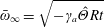 $\bar{\unicode[STIX]{x1D714}}_{\infty }=\sqrt{-\unicode[STIX]{x1D6FE}_{a}\hat{\unicode[STIX]{x1D6E9}}Rt}$
, as is visible in figure 4(a). Figure 4(b) shows that the Hopf frequency is bounded
 $(0<\bar{\unicode[STIX]{x1D714}}_{c}<\bar{\unicode[STIX]{x1D714}}_{\infty })$
at any fixed
 $Pr^{\ast }<Pr<\infty$
.
The frequency
 $\bar{\unicode[STIX]{x1D714}}_{\infty }$
is fixed by the Brunt–Väisälä frequency
 $N$
in the case of stable stratification of the fluid density (
 $\unicode[STIX]{x1D6FE}_{a}>0$
,
 $Rt<0$
), as is evident in figure 4(c). Indeed, for a fixed value of
 $Pr$
, the Hopf frequency (5.17) can be expressed via the Brunt–Väisälä frequency as
 $$\begin{eqnarray}\bar{\unicode[STIX]{x1D714}}_{c}=\sqrt{\frac{N^{2}}{2\unicode[STIX]{x1D6FA}^{2}}\frac{Pr}{Pr+1}+\frac{4(1+Ro)(1-\unicode[STIX]{x1D6FE}_{a}\hat{\unicode[STIX]{x1D6E9}})}{(Pr+1)^{2}}}.\end{eqnarray}$$
Hence, in the limit of
 $Pr\rightarrow \infty$
we have
 $$\begin{eqnarray}\bar{\unicode[STIX]{x1D714}}_{\infty }=\frac{1}{\sqrt{2}}\frac{N}{\unicode[STIX]{x1D6FA}}=\sqrt{-\frac{\unicode[STIX]{x1D6FE}_{a}}{2\ln \unicode[STIX]{x1D702}}},\end{eqnarray}$$
which, in particular, yields another expression for the Brunt–Väisälä frequency in the case of Rayleigh-unstable flows with outward heating
 $(\unicode[STIX]{x1D6FE}_{a}>0)$
:
 $$\begin{eqnarray}N^{2}=-\frac{\unicode[STIX]{x1D6FE}_{a}}{\ln \unicode[STIX]{x1D702}}\unicode[STIX]{x1D6FA}^{2}.\end{eqnarray}$$
Figure 4(c) shows that all the critical frequencies tend asymptotically to the line (6.12) as
 $N/\unicode[STIX]{x1D6FA}\rightarrow \infty$
. With a decrease in the ratio
 $N/\unicode[STIX]{x1D6FA}$
the critical frequency vanishes at the characteristic value of the Brunt–Väisälä frequency
 $N_{c}$
given by
 $$\begin{eqnarray}\frac{N_{c}^{2}}{\unicode[STIX]{x1D6FA}^{2}}=-\frac{8(1+Ro)(1-\unicode[STIX]{x1D6FE}_{a}\hat{\unicode[STIX]{x1D6E9}})}{Pr(Pr+1)}.\end{eqnarray}$$
The characteristic Brunt–Väisälä frequency
 $N_{c}$
determines the stratification that is required to excite inertial waves by the rotation. Since
 $N_{c}$
decreases with an increase in
 $Pr$
(figure 4), we conclude that the inertial waves are easier to excite in Rayleigh-unstable flow by an outward radial temperature gradient in the case of highly viscous fluids than in the case of weakly viscous fluids.
7 Discussion
The short-wavelength approximation has been used to investigate the stability of Taylor–Couette flow with a radial buoyancy force induced by coupling between a radial temperature gradient and the centrifugal force in the Boussinesq approximation. A characteristic polynomial equation has been analysed and marginal stability branches of stationary and oscillatory modes have been found analytically. The present method allows one to find the explicit dependence of the marginal state with the main control parameters:
 $Pr$
,
 $Ro$
,
 $\unicode[STIX]{x1D6FE}_{a}$
and
 $Rt$
.
The reader should be aware that for the validity of the Boussinesq approximation, the thermal expansion parameter must be very small (i.e.
 $|\unicode[STIX]{x1D6FE}_{a}|\ll 1$
) so that it is possible to neglect
 $\unicode[STIX]{x1D6FE}_{a}$
before
 $1$
in all expressions containing
 $1-\unicode[STIX]{x1D6FE}_{a}/2$
. In fact, in our computations, the largest value of
 $|\unicode[STIX]{x1D6FE}_{a}|$
was
 $|\unicode[STIX]{x1D6FE}_{a}|=0.01$
for fluids with the largest expansion coefficient found in the literature, to which a maximum of temperature difference applied should not exceed
 $\unicode[STIX]{x0394}T_{max}=5\,^{\circ }\text{C}$
.
From the above results computed at the geometric mean radius, for each value of rotating case in circular Couette flow (i.e. for a given value of
 $\unicode[STIX]{x1D707}$
), it is possible to determine the critical modes and their threshold
 $Ta_{c}$
as a function of different flow parameters
 $\unicode[STIX]{x1D702},\unicode[STIX]{x1D6FE}_{a}$
and
 $Pr$
together with the critical frequency for oscillatory modes. We have determined the critical parameters for the particular case of specific interest: sole inner cylinder rotation (
 $\unicode[STIX]{x1D707}=0$
), sole outer cylinder rotation (
 $\unicode[STIX]{x1D707}\rightarrow \infty$
), solid body rotation (
 $\unicode[STIX]{x1D707}=1$
) and Keplerian rotation (
 $\unicode[STIX]{x1D707}=\unicode[STIX]{x1D702}^{3/2}$
).
For the inner cylinder sole rotation, we have retrieved and extended the results of linear stability analysis (Meyer et al.
Reference Meyer, Yoshikawa and Mutabazi2015). For example, we have proved easily that the slope of the branch of stationary modes at the origin (
 $\unicode[STIX]{x1D6FE}_{a}=0$
) is increasing with both
 $Pr$
and
 $\unicode[STIX]{x1D702}$
. In fact, one gets
 $$\begin{eqnarray}\frac{\text{d}Ta}{\text{d}\unicode[STIX]{x1D6FE}_{a}}(\unicode[STIX]{x1D6FE}_{a}=0)=\frac{Ta_{0}}{4}\left(1-\frac{2Pr(Ta_{0})^{2}}{\ln \unicode[STIX]{x1D702}}\right).\end{eqnarray}$$
To our best knowledge, Rayleigh-stable flows (except solid body rotation) with a radial temperature gradient have never been treated analytically in such detail so far and the results presented in this work offer new predictions of convective instabilities. In the case of sole outer cylinder rotation, in the case of solid body rotation, and in the Keplerian regime, inward heating is destabilizing and leads to the oscillatory instability via Hopf bifurcation at
 $0<Pr<Pr^{H}<1$
and to stationary instability for any value
 $Pr>Pr^{S}>1$
, where the thresholds depend on
 $\unicode[STIX]{x1D6FE}_{a}$
and
 $\unicode[STIX]{x1D702}$
(table 1). The values of
 $Pr$
for which the oscillatory instability is observed are comparable to those of the astrophysical flows for which
 $Pr\approx 0.02$
. At the Rayleigh line the flow is unstable for inward heating. The present model is based on the short-wavelength approximation in the axial direction, so, strictly speaking, it cannot be applied as such to the case of solid body rotation, where it is known (Auer, Busse & Clever Reference Auer, Busse and Clever1995) that the critical modes are columnar vortices (
 $n\neq 0,k=0$
).
In appendix A we have compared the present results with those derived by Economides and Moir (Economides & Moir Reference Economides and Moir1980) for Taylor–Couette flow with a centripetal acceleration and a radial temperature gradient. Lopez et al. (Reference Lopez, Marques and Avila2013) have investigated the stability of a rotating cylindrical annulus with a negative radial temperature gradient and in the presence of gravity
 $g$
. While these authors suggested that quasi-Keplerian flows may be stable for weak stratification in the radial direction, our results show that laminar quasi-Keplerian flows may be destabilized by the centrifugal buoyancy, leading to oscillatory modes for values of
 $Pr$
relevant to accretion-disc problem, although we have considered a model that has solid radial boundaries.
8 Conclusion
The short-wavelength approximation method has been applied to the linear stability of circular Couette flow with a centrifugal buoyancy induced by a radial temperature gradient in the absence of natural gravity. The marginal states (stationary and oscillatory modes) have been determined analytically and the effects of the different parameters of the problem on flow stability have been analysed in detail. The centrifugal buoyancy enhances the instability of Rayleigh-unstable flows in inward heating, and in outward heating it induces oscillatory modes, the frequency of which can be compared with the Brunt–Väisäla frequency in the limit of large
 $Pr$
values. In inward heating it also induces instability in Rayleigh-stable flows in the form of stationary modes for large values of
 $Pr$
or oscillatory modes for small values of
 $Pr$
. The present study may serve as a theoretical guideline to linear stability analysis and to direct numerical simulations (DNS) of the flow.
Acknowledgements
O.N.K. has benefited from the CNRS grant for visiting senior scholars and acknowledges financial support from the ERC Advanced Grant ‘Instabilities and nonlocal multiscale modelling of materials’ FP7-PEOPLE-IDEAS-ERC-2013-AdG (2014-2019). I.M. is grateful to A. Meyer and Y. Harunori and O.N.K. is grateful to L. Tuckerman for fruitful exchanges on this work. I.M. acknowledges support from the French National Research Agency (ANR) through the program Investissements d’Avenir (No. ANR-10 LABX-09-01), LABEX
 $\text{EMC}^{3}$
(project TUVECO) and from the CPER Normandie.
Appendix A. Link to Economides & Moir (Reference Economides and Moir1980)
In the appendix we would like to compare our short-wavelength equations with the matrix (4.6) to the results by Economides and Moir (Economides & Moir Reference Economides and Moir1980) derived in the narrow-gap approximation.
Let
 $d=R_{2}-R_{1}\ll R_{1}$
be the size of the gap between the cylinders in the Couette cell. Then, we can write
 $$\begin{eqnarray}x=(r-R_{1})/d,\quad \unicode[STIX]{x1D707}=\unicode[STIX]{x1D6FA}_{2}/\unicode[STIX]{x1D6FA}_{1},\quad \unicode[STIX]{x1D6FA}(x)=1-(1-\unicode[STIX]{x1D707})x,\quad x\in [0,1].\end{eqnarray}$$
Denoting
 $D=\text{d}/\text{d}x$
so that
 $\text{d}/\text{d}r=d^{-1}\text{d}/\text{d}x$
we define the operators
 $$\begin{eqnarray}\displaystyle \left.\begin{array}{@{}c@{}}L=D^{2}-(k_{z}d)^{2}-\unicode[STIX]{x1D70E}-\text{i}k\sqrt{T}\unicode[STIX]{x1D6FA}(x),\\ M=D^{2}-(k_{z}d)^{2}-\unicode[STIX]{x1D70E}Pr-\text{i}kPr\sqrt{T}\unicode[STIX]{x1D6FA}(x),\end{array}\right\} & & \displaystyle\end{eqnarray}$$
where
 $Pr=\unicode[STIX]{x1D708}/\unicode[STIX]{x1D705}$
is the Prandtl number and
 $$\begin{eqnarray}\unicode[STIX]{x1D70E}=\frac{\unicode[STIX]{x1D714}d^{2}}{\unicode[STIX]{x1D708}},\quad k=m\sqrt{-\frac{\unicode[STIX]{x1D6FA}_{1}}{4A}},\quad T=-\frac{4A\unicode[STIX]{x1D6FA}_{1}d^{4}}{\unicode[STIX]{x1D708}^{2}},\quad \bar{\unicode[STIX]{x1D6FD}}=\frac{T_{2}-T_{1}}{R_{2}-R_{1}}.\end{eqnarray}$$
The temporal eigenvalue is denoted by
 $\unicode[STIX]{x1D714}$
and the azimuthal wavenumber by
 $m$
. The parameter
 $A$
is a coefficient in the expression for the background circular Couette flow
 $$\begin{eqnarray}r\unicode[STIX]{x1D6FA}(r)=Ar+\frac{B}{r}\end{eqnarray}$$
and can be expressed via the Rossby number
 $Ro$
as Kirillov et al. (Reference Kirillov, Stefani and Fukumoto2014):
 $$\begin{eqnarray}A=\unicode[STIX]{x1D6FA}(1+Ro).\end{eqnarray}$$
Then, the system of the narrow-gap equations derived in Economides & Moir (Reference Economides and Moir1980) is
 $$\begin{eqnarray}\displaystyle \left.\begin{array}{@{}c@{}}L(D^{2}-(k_{z}d)^{2})u^{\prime }=-(k_{z}d)^{2}T\unicode[STIX]{x1D6FA}(x)v^{\prime }+(k_{z}d)^{2}R\unicode[STIX]{x1D703}^{\prime },\\ Lv^{\prime }=u^{\prime },\\ M\unicode[STIX]{x1D703}^{\prime }=u^{\prime },\end{array}\right\} & & \displaystyle\end{eqnarray}$$
where (with
 $g$
denoting constant gravitational acceleration and
 $\unicode[STIX]{x1D6FC}$
the coefficient of thermal expansion)
 $$\begin{eqnarray}R=\frac{g\unicode[STIX]{x1D6FC}\bar{\unicode[STIX]{x1D6FD}}d^{4}}{\unicode[STIX]{x1D708}\unicode[STIX]{x1D705}},\quad u^{\prime }=\frac{2Ad\unicode[STIX]{x1D6FF}}{\unicode[STIX]{x1D708}\unicode[STIX]{x1D6FA}_{1}}u,\quad v^{\prime }=\frac{v}{R_{1}\unicode[STIX]{x1D6FA}_{1}},\quad \unicode[STIX]{x1D703}^{\prime }=\frac{2A\unicode[STIX]{x1D705}\unicode[STIX]{x1D703}}{\bar{\unicode[STIX]{x1D6FD}}\unicode[STIX]{x1D708}\unicode[STIX]{x1D6FA}_{1}R_{1}},\quad \unicode[STIX]{x1D6FF}=\frac{d}{R_{1}}.\end{eqnarray}$$
For any
 $w\sim \exp (\text{i}k_{r}r)$
, we have
 $$\begin{eqnarray}\displaystyle Lw & = & \displaystyle -\frac{d^{2}}{\unicode[STIX]{x1D708}}[\unicode[STIX]{x1D708}(k_{r}^{2}+k_{z}^{2})+\unicode[STIX]{x1D714}+\text{i}m\unicode[STIX]{x1D6FA}_{1}\unicode[STIX]{x1D6FA}(x)]w\nonumber\\ \displaystyle & = & \displaystyle -\frac{d^{2}}{\unicode[STIX]{x1D708}}[\unicode[STIX]{x1D708}|\boldsymbol{k}|^{2}+\unicode[STIX]{x1D714}+\text{i}m\unicode[STIX]{x1D6FA}_{1}\unicode[STIX]{x1D6FA}(x)]w\nonumber\\ \displaystyle & = & \displaystyle -\frac{d^{2}}{\unicode[STIX]{x1D708}}[\unicode[STIX]{x1D714}_{\unicode[STIX]{x1D708}}+\unicode[STIX]{x1D714}+\text{i}m\unicode[STIX]{x1D6FA}_{1}\unicode[STIX]{x1D6FA}(x)]w.\end{eqnarray}$$
Hence, if
 $u,v\sim \exp (\text{i}k_{r}r)$
the first of (A 6) becomes
 $$\begin{eqnarray}\displaystyle & & \displaystyle -\frac{d^{2}}{\unicode[STIX]{x1D708}}\left[\unicode[STIX]{x1D714}_{\unicode[STIX]{x1D708}}+\unicode[STIX]{x1D714}+\text{i}m\unicode[STIX]{x1D6FA}_{1}\unicode[STIX]{x1D6FA}(x)\right](-d^{2}|\boldsymbol{k}|^{2})\frac{2Ad\unicode[STIX]{x1D6FF}}{\unicode[STIX]{x1D708}\unicode[STIX]{x1D6FA}_{1}}u\nonumber\\ \displaystyle & & \displaystyle \qquad =-(k_{z}d)^{2}(-4A\unicode[STIX]{x1D6FA}_{1}d^{4})\frac{\unicode[STIX]{x1D6FA}(x)}{\unicode[STIX]{x1D708}^{2}R_{1}\unicode[STIX]{x1D6FA}_{1}}v+\,(k_{z}d)^{2}\frac{2Ag\unicode[STIX]{x1D6FC}d^{4}}{\unicode[STIX]{x1D708}^{2}\unicode[STIX]{x1D6FA}_{1}R_{1}}\unicode[STIX]{x1D703}.\end{eqnarray}$$
Simplifying the above expression, we find
 $$\begin{eqnarray}\displaystyle \left[\unicode[STIX]{x1D714}_{\unicode[STIX]{x1D708}}+\unicode[STIX]{x1D714}+\text{i}m\unicode[STIX]{x1D6FA}_{1}\unicode[STIX]{x1D6FA}(x)\right]u=\frac{k_{z}^{2}}{|\boldsymbol{k}|^{2}}2\unicode[STIX]{x1D6FA}_{1}\unicode[STIX]{x1D6FA}(x)\frac{d}{\unicode[STIX]{x1D6FF}R_{1}}v+\frac{k_{z}^{2}}{|\boldsymbol{k}|^{2}}\frac{d}{\unicode[STIX]{x1D6FF}R_{1}}g\unicode[STIX]{x1D6FC}\unicode[STIX]{x1D703} & & \displaystyle\end{eqnarray}$$
and finally
 $$\begin{eqnarray}\displaystyle \left[\unicode[STIX]{x1D714}_{\unicode[STIX]{x1D708}}+\unicode[STIX]{x1D714}+\text{i}m\unicode[STIX]{x1D6FA}_{1}\unicode[STIX]{x1D6FA}(x)\right]u=\frac{k_{z}^{2}}{|\boldsymbol{k}|^{2}}2\unicode[STIX]{x1D6FA}_{1}\unicode[STIX]{x1D6FA}(x)v+\frac{k_{z}^{2}}{|\boldsymbol{k}|^{2}}g\unicode[STIX]{x1D6FC}\unicode[STIX]{x1D703}, & & \displaystyle\end{eqnarray}$$
where
 $\unicode[STIX]{x1D714}_{\unicode[STIX]{x1D708}}=\unicode[STIX]{x1D708}|\boldsymbol{k}|^{2}$
.
Analogously, the second of (A 6) becomes
 $$\begin{eqnarray}-\frac{d^{2}}{\unicode[STIX]{x1D708}R_{1}\unicode[STIX]{x1D6FA}_{1}}\left[\unicode[STIX]{x1D714}_{\unicode[STIX]{x1D708}}+\unicode[STIX]{x1D714}+\text{i}m\unicode[STIX]{x1D6FA}_{1}\unicode[STIX]{x1D6FA}(x)\right]v=\frac{2Ad\unicode[STIX]{x1D6FF}}{\unicode[STIX]{x1D708}\unicode[STIX]{x1D6FA}_{1}}u.\end{eqnarray}$$
Simplifying it, we get
 $$\begin{eqnarray}\left[\unicode[STIX]{x1D714}_{\unicode[STIX]{x1D708}}+\unicode[STIX]{x1D714}+\text{i}m\unicode[STIX]{x1D6FA}_{1}\unicode[STIX]{x1D6FA}(x)\right]v=-2Au\end{eqnarray}$$
and, finally
 $$\begin{eqnarray}\left[\unicode[STIX]{x1D714}_{\unicode[STIX]{x1D708}}+\unicode[STIX]{x1D714}+\text{i}m\unicode[STIX]{x1D6FA}_{1}\unicode[STIX]{x1D6FA}(x)\right]v=-2\unicode[STIX]{x1D6FA}(1+Ro)u.\end{eqnarray}$$
Now, for the third of (A 6) we find
 $$\begin{eqnarray}\left[-k_{r}^{2}d^{2}-(k_{z}d)^{2}-\unicode[STIX]{x1D70E}Pr-\text{i}kPr\sqrt{T}\unicode[STIX]{x1D6FA}(x)\right]\frac{2A\unicode[STIX]{x1D705}}{\bar{\unicode[STIX]{x1D6FD}}\unicode[STIX]{x1D708}\unicode[STIX]{x1D6FA}_{1}R_{1}}\unicode[STIX]{x1D703}=\frac{2Ad\unicode[STIX]{x1D6FF}}{\unicode[STIX]{x1D708}\unicode[STIX]{x1D6FA}_{1}}u,\end{eqnarray}$$
and equivalently,
 $$\begin{eqnarray}\left[-\unicode[STIX]{x1D705}k_{r}^{2}-\unicode[STIX]{x1D705}k_{z}^{2}-\unicode[STIX]{x1D714}-\text{i}m\unicode[STIX]{x1D6FA}_{1}\unicode[STIX]{x1D6FA}(x)\right]\frac{d}{\bar{\unicode[STIX]{x1D6FD}}\unicode[STIX]{x1D708}R_{1}}\unicode[STIX]{x1D703}=\frac{\unicode[STIX]{x1D6FF}}{\unicode[STIX]{x1D708}}u,\end{eqnarray}$$
so that finally
 $$\begin{eqnarray}\left[\unicode[STIX]{x1D714}_{\unicode[STIX]{x1D705}}+\unicode[STIX]{x1D714}+\text{i}m\unicode[STIX]{x1D6FA}_{1}\unicode[STIX]{x1D6FA}(x)\right]\unicode[STIX]{x1D703}=-\bar{\unicode[STIX]{x1D6FD}}u,\end{eqnarray}$$
where
 $\unicode[STIX]{x1D714}_{\unicode[STIX]{x1D705}}=\unicode[STIX]{x1D705}|\boldsymbol{k}|^{2}$
.
We can denote
 $\unicode[STIX]{x1D6FA}=\unicode[STIX]{x1D6FA}_{1}\unicode[STIX]{x1D6FA}(x)$
and write the three equations in the matrix form
 $$\begin{eqnarray}\left(\begin{array}{@{}ccc@{}}\unicode[STIX]{x1D714}_{\unicode[STIX]{x1D708}}+\unicode[STIX]{x1D714}+\text{i}m\unicode[STIX]{x1D6FA} & -\displaystyle \frac{k_{z}^{2}}{|\boldsymbol{k}|^{2}}2\unicode[STIX]{x1D6FA} & -\displaystyle \frac{k_{z}^{2}}{|\boldsymbol{k}|^{2}}g\unicode[STIX]{x1D6FC}\\ 2\unicode[STIX]{x1D6FA}(1+Ro) & \unicode[STIX]{x1D714}_{\unicode[STIX]{x1D708}}+\unicode[STIX]{x1D714}+\text{i}m\unicode[STIX]{x1D6FA} & 0\\ \bar{\unicode[STIX]{x1D6FD}} & 0 & \unicode[STIX]{x1D714}_{\unicode[STIX]{x1D705}}+\unicode[STIX]{x1D714}+\text{i}m\unicode[STIX]{x1D6FA}\end{array}\right)\left(\begin{array}{@{}c@{}}u\\ v\\ \unicode[STIX]{x1D703}\end{array}\right)=0.\end{eqnarray}$$
In fact,
 $\bar{\unicode[STIX]{x1D6FD}}=(T_{2}-T_{1})/(R_{2}-R_{1})$
is a ‘derivative’ of the temperature with respect to radius and in the local approximation we can replace it with
 $\unicode[STIX]{x1D6E9}^{\prime }=\text{d}\unicode[STIX]{x1D703}_{0}/\text{d}r$
. Then, we can denote
 $\unicode[STIX]{x1D6FD}=(k_{z}/|\boldsymbol{k}|)$
and write
 $$\begin{eqnarray}\left(\begin{array}{@{}ccc@{}}\unicode[STIX]{x1D714}_{\unicode[STIX]{x1D708}}+\unicode[STIX]{x1D714}+\text{i}m\unicode[STIX]{x1D6FA} & -2\unicode[STIX]{x1D6FA}\unicode[STIX]{x1D6FD}^{2} & -\unicode[STIX]{x1D6FC}g\unicode[STIX]{x1D6FD}^{2}\\ 2\unicode[STIX]{x1D6FA}(1+Ro) & \unicode[STIX]{x1D714}_{\unicode[STIX]{x1D708}}+\unicode[STIX]{x1D714}+\text{i}m\unicode[STIX]{x1D6FA} & 0\\ \unicode[STIX]{x1D6E9}^{\prime } & 0 & \unicode[STIX]{x1D714}_{\unicode[STIX]{x1D705}}+\unicode[STIX]{x1D714}+\text{i}m\unicode[STIX]{x1D6FA}\end{array}\right)\left(\begin{array}{@{}c@{}}u\\ v\\ \unicode[STIX]{x1D703}\end{array}\right)=0.\end{eqnarray}$$
For the stationary axisymmetric instability the Bilharz criterion (Bilharz Reference Bilharz1944) applied to the characteristic polynomial of the matrix on the left-hand side of (A 19) yields:
 $$\begin{eqnarray}4(Ro+1)+Pr\frac{g}{\unicode[STIX]{x1D6FA}^{2}}\frac{2Rt\unicode[STIX]{x1D6E9}\unicode[STIX]{x1D6FC}}{r}+\frac{1}{Ta^{2}}>0\end{eqnarray}$$
With
 $g=\unicode[STIX]{x1D6FA}^{2}r$
, and taking into account that the sign of
 $\unicode[STIX]{x1D6FC}$
in Economides & Moir (Reference Economides and Moir1980) is opposite to the sign of
 $\unicode[STIX]{x1D6FC}$
in (2.1), we reduce the above equation to the form
 $$\begin{eqnarray}4(Ro+1)-2PrRt\hat{\unicode[STIX]{x1D6E9}}\unicode[STIX]{x1D6FE}_{a}+\frac{1}{Ta^{2}}>0,\end{eqnarray}$$
which differs from the condition (5.11) only by the factor
 $1-\unicode[STIX]{x1D6FE}_{a}\hat{\unicode[STIX]{x1D6E9}}$
at the first term. The reason for this discrepancy is that in Economides & Moir (Reference Economides and Moir1980)
 $g$
is assumed to be a constant radial gravitational acceleration whereas in Meyer et al. (Reference Meyer, Yoshikawa and Mutabazi2015) it is the centrifugal acceleration that depends on radius. Hence, substitution of
 $g=\unicode[STIX]{x1D6FA}^{2}r$
into (A 20) is not justified. On the other hand, the factor
 $1-\unicode[STIX]{x1D6FE}_{a}\hat{\unicode[STIX]{x1D6E9}}$
is small in the Boussinesq approximation, and consequently (5.11) and (A 21) can be considered as equivalent.
Taking into account that in the Boussinesq approximation the squared Brunt–Väisälä frequency is
 $N^{2}=-2\unicode[STIX]{x1D6FE}_{a}\hat{\unicode[STIX]{x1D6E9}}Rt\unicode[STIX]{x1D6FA}^{2}$
, we transform (A 21) as
 $$\begin{eqnarray}4(Ro+1)+Pr\frac{N^{2}}{\unicode[STIX]{x1D6FA}^{2}}+\frac{1}{Ta^{2}}>0.\end{eqnarray}$$
With the opposite sign the inequality (A 22) is the onset of the double-diffusive Goldreich–Schubert–Fricke instability in the form derived in Acheson & Gibbons (Reference Acheson and Gibbons1978).