2.1 Sears and Atassi formulations

Both transfer functions relate the unsteady lift $L_{dyn}$ from the gust–airfoil interaction to the quasi-steady lift $L_{qs}$ , or the lift amplitude that would result from the same range of gust angles of attack in steady flow. They take the form

(2.1) $$\begin{eqnarray}\displaystyle h_{L}={\displaystyle \frac{L_{dyn}}{L_{qs}}}={\displaystyle \frac{\hat{L}_{dyn}}{\hat{L}_{qs}}}\text{e}^{\text{i}\unicode[STIX]{x1D719}}, & & \displaystyle\end{eqnarray}$$

where hats denote amplitudes and $\unicode[STIX]{x1D719}$ represents the phase shift between the dynamic and quasi-steady lift-force signals. The time phase of the gust is taken to be positive, in accordance with Atassi (Reference Atassi1984). The dynamic lift in the Sears function is computed as a combination of quasi-steady, apparent-mass and wake-circulation lift components. The Atassi function adds contributions from distortions of the flow field due to camber and mean angle of attack to the dynamic lift from the Sears function. Thus, the two theories are quite similar; the Atassi function is simply an extension of the Sears function.

2.2 Influence of the streamwise reduced frequency $k_{2}$

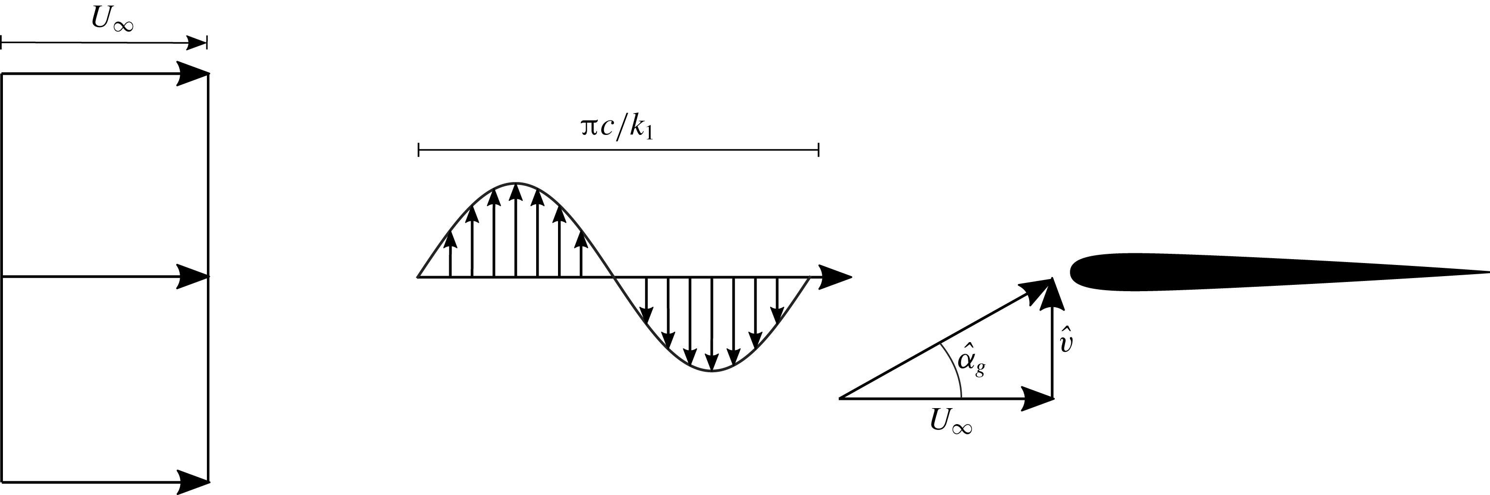
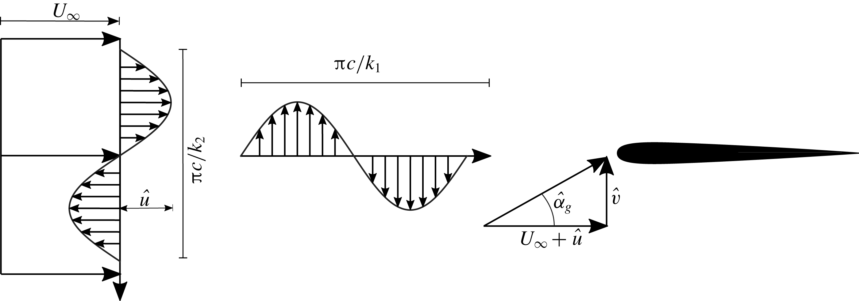
The most obvious difference between the theories of Sears and Atassi lies in the set-up of the problem to be modelled. The Sears function involves only periodic velocity fluctuations in the component normal to the airfoil ( $v$ ), as shown in figure 1. The theory of Atassi, in contrast, also includes periodic velocity fluctuations in the streamwise velocity component $u$ . These fluctuations, shown in figure 2, are characterized according to Atassi’s notation by the reduced frequency $k_{2}$ , and the vertical-velocity oscillations corresponding to those of the theory of Sears by the reduced frequency $k_{1}$ . The waveform of these streamwise fluctuations runs normal to the airfoil at a velocity of $u=\unicode[STIX]{x03C0}(fc/k_{2})$ ( $\text{m}~\text{s}^{-1}$ ), so that the streamwise velocity at any height in the flow fluctuates about the free-stream velocity with an amplitude of $\hat{u}$ . When $k_{2}$ is zero, the streamwise velocity fluctuations are not present, and the Atassi problem reduces to that of Sears.

Figure 1.

Inflow conditions according to Sears. Fluctuations in the normal velocity component $\hat{v}$ with reduced frequency $k_{1}$ impinge on the airfoil. The resulting angle-of-attack variations are represented by $\hat{\unicode[STIX]{x1D6FC}}_{g}$ .

Figure 2.

Inflow conditions according to Atassi. In addition to the normal-velocity fluctuations from the Sears problem, streamwise-velocity fluctuations with amplitude $\hat{u}$ and reduced frequency $k_{2}$ are also present. This extra gust profile is mathematically coupled with the Sears-problem gust.

This is made explicit in the mathematical definition of the Atassi function. If the Sears function is denoted as $S(k_{1})$ , the Atassi function can be written as

(2.2) $$\begin{eqnarray}\displaystyle h_{L}(k_{1},k_{2})={\displaystyle \frac{k_{1}}{|k|}}S(k_{1})+\unicode[STIX]{x1D6FC}_{\unicode[STIX]{x1D6FD}}h_{\unicode[STIX]{x1D6FD}}(k_{1},k_{2})+\unicode[STIX]{x1D6FC}_{m}h_{m}(k_{1},k_{2}), & & \displaystyle\end{eqnarray}$$

where $|k|=\sqrt{{k_{1}}^{2}+{k_{2}}^{2}}$ , $\unicode[STIX]{x1D6FC}_{\unicode[STIX]{x1D6FD}}$ is the mean angle of attack of the airfoil and $\unicode[STIX]{x1D6FC}_{m}$ is the airfoil camber, representing the deviation of the camber line from the symmetric case. $h_{\unicode[STIX]{x1D6FD}}$ and $h_{m}$ are both relatively complicated functions of $k_{1}$ and $k_{2}$ and are defined in Atassi (Reference Atassi1984). Both functions become zero when $k_{2}$ is zero. Additionally, for the purposes of this work, only unloaded airfoils, i.e. at zero mean angle of attack ( $\unicode[STIX]{x1D6FC}_{\unicode[STIX]{x1D6FD}}=0$ ) and with zero camber ( $\unicode[STIX]{x1D6FC}_{m}=0$ ) are considered, so that these terms do not contribute to the Atassi function $h_{L}$ . From this definition, it is evident that the Atassi function is distinct from the Sears function if and only if $k_{2}\neq 0$ . Furthermore, for a symmetric airfoil at zero mean angle of attack, the Atassi function is directly related to the Sears function,

(2.3) $$\begin{eqnarray}\displaystyle A(k_{1},k_{2})={\displaystyle \frac{k_{1}}{|k|}}S(k_{1}). & & \displaystyle\end{eqnarray}$$

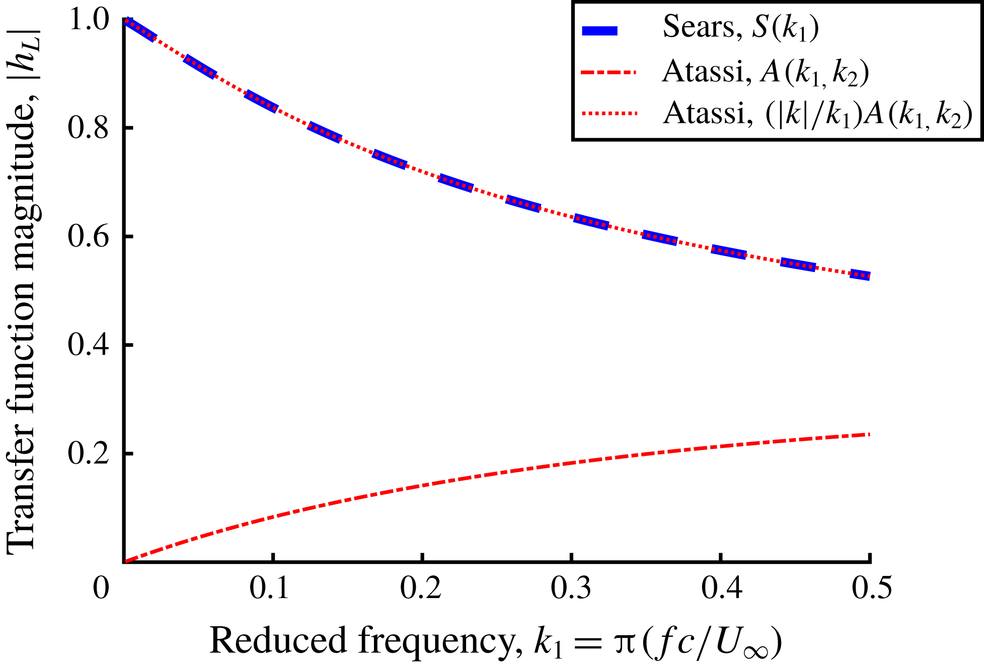
Thus, the factor $k_{1}/|k|$ allows the Atassi and Sears functions to be directly compared. The profiles of these two functions are shown in figure 3. Without this adjustment factor, the Atassi function starts from zero at $k_{1}=0$ and increases monotonically. When $A(k_{1},k_{2})$ is multiplied by the adjustment factor, the Sears function is retrieved. Neither the camber correction term $h_{m}$ nor the angle-of-attack correction term $h_{\unicode[STIX]{x1D6FD}}$ factors into this comparison. This emphasizes the point that the fundamental difference between the theories of Sears and Atassi lies not in the corrections for flow-field distortion in the presence of the airfoil, as Cordes et al. (Reference Cordes, Kampers, Meißner, Tropea, Peinke and Hölling2017) hypothesized, but rather in the additional gust parameter $k_{2}$ .

Figure 3.

Profiles of the Sears and Atassi functions. The Atassi curve is given for $k_{2}=1$ . When $k_{2}$ is zero, or when $A(k_{1},k_{2})$ is multiplied by $|k|/k_{1}$ , the Atassi function collapses onto the Sears function. The phase remains the same irrespective of the value of $k_{2}$ .

2.3 Transfer-function normalization

The importance of the $k_{2}$ parameter becomes more evident when the normalizations of the two transfer functions are scrutinized. These factors are not used to compute the transfer functions themselves, but rather to normalize the unsteady lift-force data obtained from gust-response experiments ( $\hat{L}_{dyn}$ ). They are therefore measures of the quasi-steady lift ( $\hat{L}_{qs}$ ), which by definition must include a parameter to represent the strength of the unsteady gust fluctuations. For the Sears function, the factor is given by the relation

(2.4) $$\begin{eqnarray}\displaystyle \hat{L}_{qs}=\unicode[STIX]{x03C0}\unicode[STIX]{x1D70C}cU_{\infty }\hat{v}\approx \unicode[STIX]{x03C0}\unicode[STIX]{x1D70C}cU_{\infty }^{2}\hat{\unicode[STIX]{x1D6FC}}_{g}, & & \displaystyle\end{eqnarray}$$

where $\hat{v}$ is the amplitude of the velocity fluctuations normal to the airfoil. Since $\hat{v}\ll U_{\infty }$ , $\hat{v}$ can be approximated as being directly proportional to $\hat{\unicode[STIX]{x1D6FC}}_{g}$ , the amplitude of the inflow angles of attack created by the gust. From this normalization, it is clear that the Sears function should be independent of the gust strength $\hat{v}$ and thus also independent of the gust-angle amplitude $\hat{\unicode[STIX]{x1D6FC}}_{g}$ .

Defining a gust strength is made more difficult when the streamwise gust defined by $k_{2}$ is introduced. In Atassi’s theory, a single parameter $\unicode[STIX]{x1D716}$ represents simultaneously the gust strength of the normal and streamwise-velocity fluctuations. The amplitudes of the gusts in the streamwise and normal-velocity components are given respectively as $\hat{u} =U_{\infty }\unicode[STIX]{x1D716}k_{2}/|k|$ and $\hat{v}=U_{\infty }\unicode[STIX]{x1D716}k_{1}/|k|$ (cf. figure 2). The gust strength is defined such that $\unicode[STIX]{x1D716}\ll 1$ , implying that $\hat{u} \ll U_{\infty }$ and $\hat{v}\ll U_{\infty }$ . This allows the gust strengths from the theories of Sears and Atassi to be compared via the physical quantity $\hat{\unicode[STIX]{x1D6FC}}_{g}$ . The gust-angle amplitude can thus be represented as

(2.5) $$\begin{eqnarray}\displaystyle \hat{\unicode[STIX]{x1D6FC}}_{g}=\arctan \left({\displaystyle \frac{\hat{v}}{U_{\infty }+\hat{u} }}\right)\approx \arctan \left({\displaystyle \frac{\hat{v}}{U_{\infty }}}\right)\approx \unicode[STIX]{x1D716}{\displaystyle \frac{k_{1}}{|k|}}. & & \displaystyle\end{eqnarray}$$

When $k_{2}$ is zero, the gust strength $\unicode[STIX]{x1D716}$ is simply $\hat{\unicode[STIX]{x1D6FC}}_{g}$ , as for the Sears function. When $k_{2}$ takes a non-zero value, a constant value of $\unicode[STIX]{x1D716}$ means that $\hat{\unicode[STIX]{x1D6FC}}_{g}$ becomes a monotonically increasing function of $k_{1}$ . Thus, the gust strength in the Atassi problem is not strictly tied to the physical quantity $\hat{\unicode[STIX]{x1D6FC}}_{g}$ . This is important for the normalization of the Atassi function, given by

(2.6) $$\begin{eqnarray}\displaystyle \hat{L}_{qs}=\unicode[STIX]{x03C0}\unicode[STIX]{x1D70C}c{U_{\infty }}^{2}\unicode[STIX]{x1D716}. & & \displaystyle\end{eqnarray}$$

Since the factor $|k|/k_{1}$ appears in (2.5), exchanging $\unicode[STIX]{x1D716}$ for $\hat{\unicode[STIX]{x1D6FC}}_{g}$ in this normalization is mathematically equivalent to applying the adjustment factor from (2.3). This confirms that the Sears and Atassi functions are related by a factor of $|k|/k_{1}$ , which is already evident from (2.2). In this work, both normalizations for the Atassi function are considered, in order to demonstrate that they are both valid.

The normalizations of the transfer functions thus allow a wide range of experimental conditions to be captured by a single curve defined only by $k_{2}$ , provided that the parameters $k_{2}$ , $\hat{\unicode[STIX]{x1D6FC}}_{g}$ and by extension $\unicode[STIX]{x1D716}$ , can be controlled and measured accurately.

2.4 Significance for experiments

The mathematical details outlined above are important considerations for the set-up of experiments investigating the Sears and Atassi problems. They show that control over the fluctuations in the streamwise velocity is required for the comparison of the transfer functions. Thus, to reproduce the conditions of the Sears problem, $\hat{u}$ must be kept as small as possible so that $k_{2}$ can be set to zero. If this condition is not taken into account, then the resulting conditions will be those of the Atassi problem and not strictly those of Sears. No previous study has considered systematically controlling the oscillations in $u$ while performing Sears measurements, and therefore a central goal of this study is to demonstrate the importance of this distinction in an experimental context.

In addition, in order to compute experimental transfer-function values from unsteady lift-force data, the parameter $\hat{\unicode[STIX]{x1D6FC}}_{g}$ must be accurately determined, and the correct normalizations for the transfer functions in question must be employed. In previous studies (e.g. Cordes et al. Reference Cordes, Kampers, Meißner, Tropea, Peinke and Hölling2017), the proper normalization for the transfer functions had not been clarified, and $\hat{\unicode[STIX]{x1D6FC}}_{g}$ was not characterized over the entire range of experimental gust conditions. If data are to be compared directly with the Atassi function, values for the parameters $k_{2}$ and $\unicode[STIX]{x1D716}$ must also be known. These can be difficult to quantify accurately in experiments. All of these considerations must be accounted for in experiments seeking to compare the two transfer functions.

The transfer-function phase profiles for the Sears and Atassi functions are identical when camber and mean angle of attack are both zero, irrespective of the values of $k_{2}$ , $\unicode[STIX]{x1D716}$ , and $\hat{\unicode[STIX]{x1D6FC}}_{g}$ . Therefore, the phase is not considered in detail here.

3.1 Wind tunnel and grid

The experiments reported in this study were carried out in a closed-loop wind tunnel at the University of Oldenburg, details of which are given in Knebel, Kittel & Peinke (Reference Knebel, Kittel and Peinke2011). The test section had a cross-sectional profile of $1.00\times 0.80~\text{m}^{2}$ . An active grid was installed in the tunnel at the front of the test section, 1.1 m upstream from the quarter-chord point of the airfoil. It was composed of nine three-dimensionally printed vanes, each with a NACA 0016 cross-sectional profile with 71 mm chord and $0.8~\text{m}$ span. The turbulence intensity in the middle of the tunnel, computed from data from hot-wire anemometers, was less than $0.3\,\%$ . 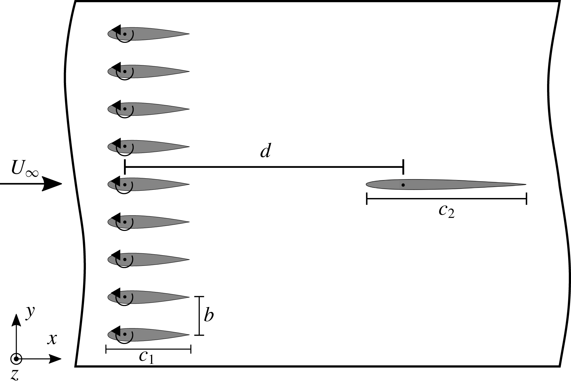The vanes were pitched about their quarter-chord point in sinusoidal profiles. The precise details of the motion protocols employed in this study are given below in § 4.2. A schematic of the wind tunnel and active grid is provided in figure 4.

Figure 4.

Schematic showing the set-up of the wind tunnel and active grid (illustration not to scale). The distance between the grid and the quarter-chord point of the test airfoil is $d=1.1~\text{m}$ . The vanes of the active grid have a chord length of $c_{1}=71~\text{mm}$ .

A NACA 0006 airfoil with a $202~\text{mm}$ chord and $800~\text{mm}$ span was constructed at the TU Darmstadt and served as a test airfoil. It was composed of two carbon-fibre shells attached to an aluminium spine, so that the airfoil was both smooth and rigid against torsion. This profile was selected to conform to the thin-airfoil assumption of Sears, based on predictions from the XFOIL software (cf. Drela Reference Drela1989) for the range of angles of attack the airfoil could encounter without incurring flow separation on the surface. A thin strip of fluorescent foil at the location of the laser sheet reduced surface reflections when particle image velocimetry (PIV) measurements were performed.

3.2 Hot-wire measurements

To obtain empirical relations between the grid amplitude $\hat{\unicode[STIX]{x1D703}}$ and gust-angle amplitude $\hat{\unicode[STIX]{x1D6FC}}$ over the range of potential experimental flow conditions, as well as estimates for the Atassi gust parameters $\unicode[STIX]{x1D716}$ and $k_{2}$ , a large parameter space of grid amplitudes and reduced frequencies was traversed for two distinct grid configurations (detailed in § 4.2). Data were collected using a CTA System from DANTEC DYNAMICS, consisting of a StreamLine Automatic Calibrator for X-wire calibration, a StreamLine frame with two CTA modules, a $6~\text{mm}$ short support of type 55H24 and an X-wire of type 55P51.

During the characterization of the inflow the calibrated X-wire was placed in at the centreline of the empty wind tunnel at the intended leading edge position of the airfoil 1 m downstream of the active grid. For each frequency and amplitude 40 000 values were taken at a sampling frequency of 20 kHz resulting in a duration of 20 s per grid protocol. To cover a broad range of possible reduced frequencies and gust amplitudes, the grid was characterized for frequencies from 1 to 10 Hz with grid amplitudes from $2.5^{\circ }$ up to $20^{\circ }$ for free-stream velocities between $15$ and $25~\text{m}~\text{s}^{-1}$ .

3.3 Force measurements

A pair of K3D120 3-axis force balances and a TS110 moment sensor from ME-Messsysteme allowed forces and moments to be measured at the airfoil’s quarter-chord point. Thirty seconds of force data were collected for each measurement. All measurements, including measurements with the PIV system, were started simultaneously via a trigger provided two seconds after the active-grid protocol was started.

To compute transfer functions from experimental data, the force data were first shifted from the airfoil frame of reference to that of the wind tunnel. The first two seconds of each data set were discarded in order to remove start-up effects. A Fourier transform of the signal yielded the magnitude of the lift-force fluctuations, corresponding to $\hat{L}_{dyn}$ from (2.1). For the Sears function, the quasi-steady lift amplitude $\hat{L}_{qs}$ was interpolated from steady lift curves $L_{U_{\infty }}$ using the relation

(3.1) $$\begin{eqnarray}\displaystyle \hat{L}_{qs}=f(U_{\infty },\hat{\unicode[STIX]{x1D6FC}}_{g},\unicode[STIX]{x1D6FC}_{m})={\textstyle \frac{1}{2}}(L_{U_{\infty }}(\unicode[STIX]{x1D6FC}_{m}+\hat{\unicode[STIX]{x1D6FC}}_{g})-L_{U_{\infty }}(\unicode[STIX]{x1D6FC}_{m}-\hat{\unicode[STIX]{x1D6FC}}_{g})). & & \displaystyle\end{eqnarray}$$

Because $\unicode[STIX]{x1D6FC}_{m}$ in these experiments was always zero, this was approximately equivalent to

(3.2) $$\begin{eqnarray}\displaystyle \hat{L}_{qs}={\displaystyle \frac{\unicode[STIX]{x2202}L_{U_{\infty }}}{\unicode[STIX]{x2202}\unicode[STIX]{x1D6FC}}}\hat{\unicode[STIX]{x1D6FC}}_{g}, & & \displaystyle\end{eqnarray}$$

where $\unicode[STIX]{x2202}L_{U_{\infty }}/\unicode[STIX]{x2202}\unicode[STIX]{x1D6FC}$ represents the lift slope of the airfoil as computed from a fit of the linear portion of the steady lift curve. This is the experimental equivalent of the ideal quasi-steady lift factor given in (2.4), since a value for the lift slope that reflected the test airfoil used in experiments was preferable to the theoretical lift slope $\unicode[STIX]{x03C0}\unicode[STIX]{x1D70C}c{U_{\infty }}^{2}$ . This modified form was used to compute $\hat{L}_{qs}$ for the Atassi function, with $\unicode[STIX]{x1D716}$ substituted for $\hat{\unicode[STIX]{x1D6FC}}_{g}$ . Here $\unicode[STIX]{x1D716}$ was computed from (2.5). To compare the Atassi function directly with the Sears function, the quasi-steady lift expression given in (3.2) was used instead of relying on values of $\unicode[STIX]{x1D716}$ and $k_{2}$ , which were not measured directly.

The data points were validated using both force-balance data and, for the six cases in which stereo PIV was employed, phase-averaged velocity vector fields. Error bars were computed from the standard deviation of the phase-averaged lift-force signal and the standard deviation of the gust-angle amplitudes from hot-wire data. For data taken at $U_{\infty }=10~\text{m}~\text{s}^{-1}$ , no hot-wire data were available, and therefore gust-angle amplitudes were extracted from the stereo PIV vector fields and errors were estimated.

3.4 PIV set-up

To investigate the spatial and temporal structures occurring in the flow, PIV measurements were additionally performed. The PIV set-up was a stereoscopic set-up from LaVision, composed of two Phantom Miro 320S high-speed cameras operated at a frame rate of 500 Hz. This reduced temporal resolution and a RAM size of the cameras of 12 GB enabled a total measurement time of 5.5 s. The cameras were mounted above and below the test section. A Litron LDY-303HE Nd:YLF dual-cavity high-speed pulsed laser illuminated the suction side of the airfoil from the rear of the tunnel. Images were recorded and evaluated with LaVision’s DaVis 8.4 software with $16\times 16$ pixel interrogation areas, 50 % overlap, and outlier interpolation.

3.5 Numerical set-up

Numerical simulations of the flow field in the wind tunnel were performed with the aim of complementing the experimental measurements. Two configurations were studied, corresponding to two different inflow conditions. The first configuration corresponded to conditions specified by Sears (see figure 1) and simulated the flow past a NACA 0006 airfoil with chord length $c_{2}=0.2~\text{m}$ . The second simulation involved only the nine oscillatory vanes without an airfoil model and was aimed at reproducing the tunnel unsteadiness as encountered in the experiments (see figure 4).

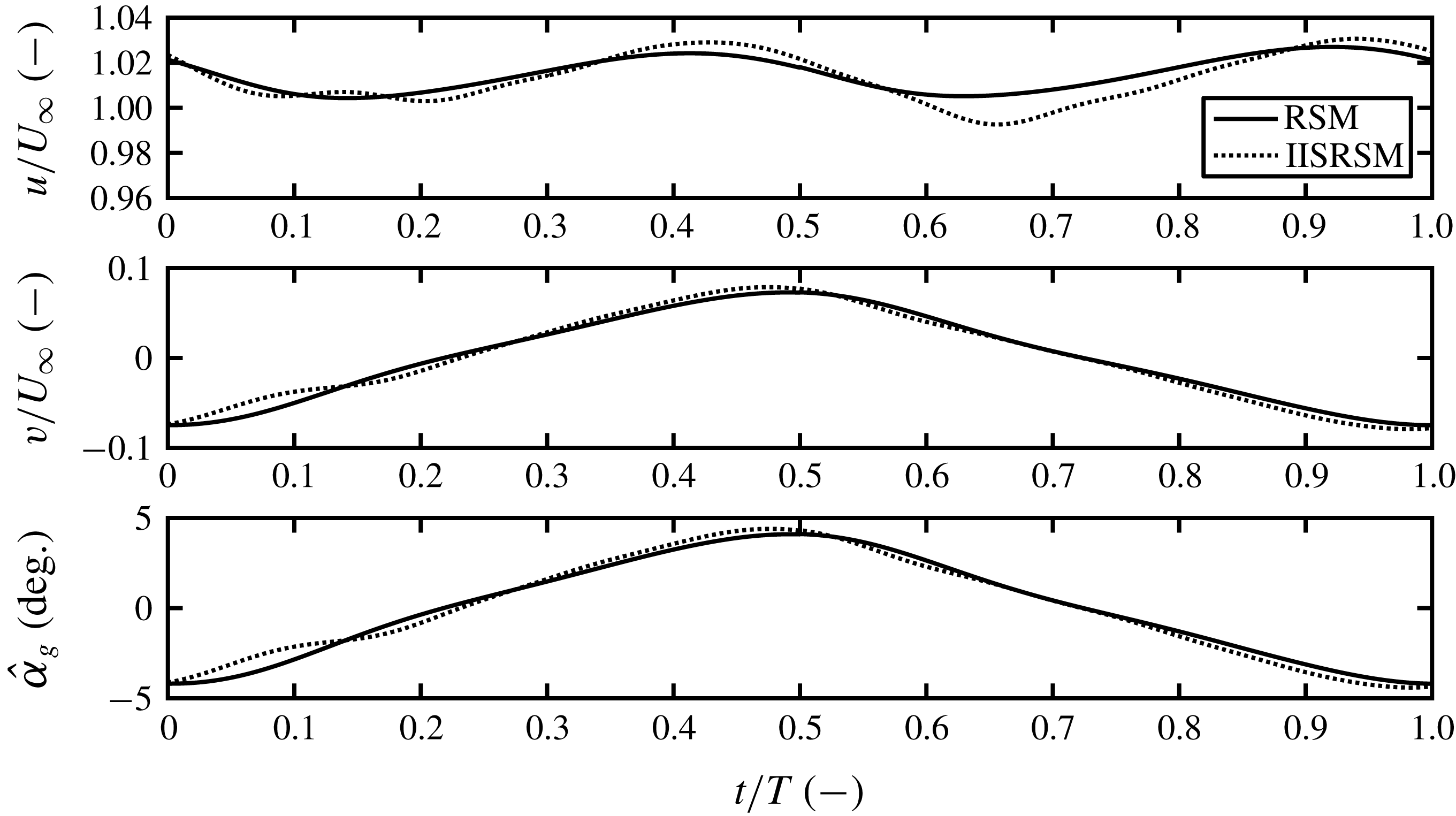
The computations were performed within the unsteady RANS (Reynolds-averaged Navier–Stokes) computational framework employing the baseline and eddy-resolving versions of the near-wall Reynolds-stress model (RSM) by Jakirlic & Hanjalic (Reference Jakirlic and Hanjalic2002). The model is capable of asymptotically capturing both the strengthened viscosity effects and the kinematic wall blocking. The latter model property is expressed in terms of both Reynolds-stress and stress-dissipation anisotropies coping with correct asymptotic behaviour of all turbulence quantities when approaching the wall. Unlike the baseline model, its eddy-resolving formulation (denoted improved instability sensitive RSM – IISRSM) is capable of resolving the fluctuating turbulence. This model feature, created in line with the scale-adaptive simulation (SAS) methodology proposed originally by Menter & Egorov (Reference Menter and Egorov2010) in conjunction with their shear-stress transport (SST) eddy-viscosity model of turbulence, is achieved by suppressing the modelled turbulence towards a corresponding sub-scale level. The characteristic size of the unresolved sub-scale turbulent eddies is proportional to the von Kármán length scale (comprising the second derivative of the velocity field: $\unicode[STIX]{x1D6FB}^{2}\boldsymbol{U}$ ), which mimics, analogously to the grid spacing $\unicode[STIX]{x1D6E5}$ in large-eddy simulation (LES), the relevant length scale of the SAS-related residual turbulence. The turbulence suppression in the SAS modelling framework is achieved by introducing an additional production term ( $P_{SAS}$ ) into the scale-supplying equation governing the $\unicode[STIX]{x1D714}$ -quantity (with $\unicode[STIX]{x1D714}\propto \unicode[STIX]{x1D700}/k$ representing inverse turbulent time scale). Herewith, an appropriate enhancement of the turbulence activity originating from the resolved motion, especially within the shear layer regions, is ensured; interested readers are referred to Jakirlić & Maduta (Reference Jakirlić and Maduta2015) and Maduta, Ullrich & Jakirlic (Reference Maduta, Ullrich and Jakirlic2017) for more details.

The model equations are implemented into the open source toolbox OpenFOAM^® with which all present simulations were performed. The code employs a finite-volume discretization method based on the integral form of the general conservation law applied in conjunction with block-structured grid arrangements. The flow domains considered are meshed by the OpenFOAM^® relevant utility denoted as ‘blockMesh’. The temporal resolution adopted guarantees a Courant number smaller than one in the entire solution domain. The discretization of the convection terms is achieved using a blended central differencing scheme implemented in the differed-correction approach manner. This methodology is considered adequate in view of a fine grid used in the regions with high gradients.

The first computational set-up is concerned with the flow past a NACA 0006 airfoil. The inflow cross-section is positioned immediately downstream of the active grid. The incoming gusty flow conditions are represented by a time-dependent sinusoidal velocity condition at the inlet (compare with figure 1). The two-dimensional solution domain (not shown here) with the inflow plane located at 1.1 m upstream of the test airfoils quarter-chord point (figure 4) and the outlet plane located at 1.5 m downstream of the airfoils quarter-chord point, is meshed with 59 300 hexahedral grid cells. The grid is squeezed with an adequate grading towards the airfoil surface. The governing equations are integrated to the walls; the wall-adjacent computational node at the airfoil is situated deep within the viscous sublayer, ensuring the value of the dimensionless wall distance $y^{+}\leqslant 1$ . Such a fine grid resolution is necessary for applying the exact wall boundary conditions, formulated in relation to the physically correct behaviour of the mean flow and turbulent quantities. The upper and lower bounding of the solution domain is represented by symmetry planes positioned equidistantly at 0.5 m from the airfoil’s chord line. Application of the symmetry conditions is justified as they do not influence the flow around the airfoil. These computations were performed employing the baseline RSM. The credibility of performing two-dimensional computations is based on the experience gained by computing the flow in the empty plenum (the second configuration). These results, obtained for both two-dimensional and three-dimensional computations, exhibit no noticeable difference (see figure 5 and associated discussion).

Figure 5.

Computationally obtained time variation of the streamwise and normal component of the mean velocity field and gust-angle amplitude by using baseline and eddy-resolving Reynolds-stress models.

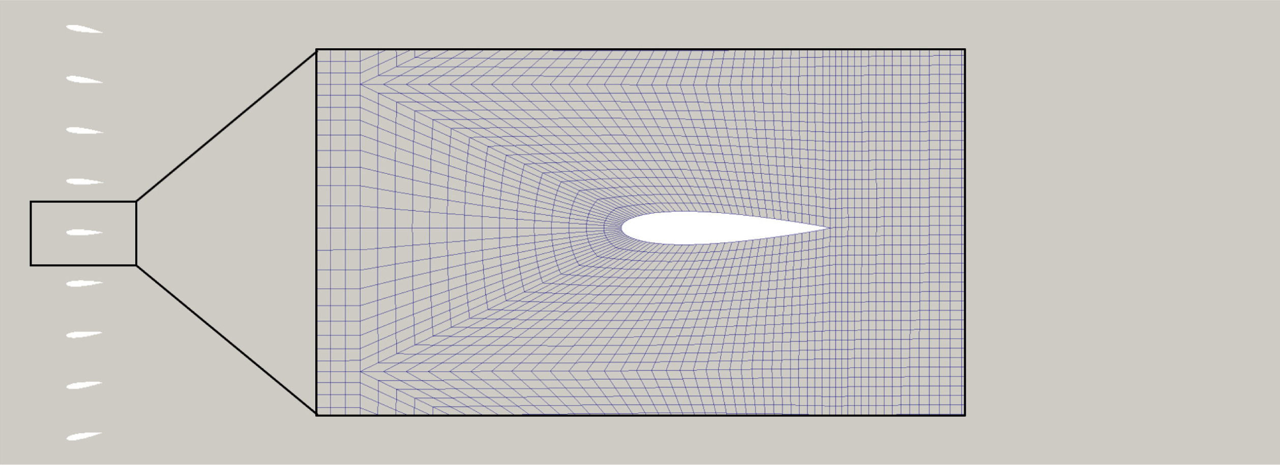
The second configuration deals with the entire plenum (accounting also for the plenum walls) without the NACA 0006 airfoil, but including the active grid consisting of nine symmetric airfoil-like vanes, (figure 6). The corresponding inflow conditions are realized by the oscillatory motion of the vanes using a dynamic meshing utility. This utility is based on the so-called ‘space conservation law’, implying the conservation of the grid cell number during the oscillatory vane motion. Accordingly, an additional equation describing the conservation of space is solved simultaneously with the continuity and momentum equations as well as with equations governing the turbulence quantities. The length of the solution domain accommodating the nine vanes is 2.8 m (see figure 6), where the zero-gradient outflow boundary conditions were applied. The spanwise extent of the solution domain amounts to 50 % of the NACA 0006 airfoil chord. The fully hexahedral grid consisted of 112 736 cells in the central vertical plane. The three-dimensional computational domain was meshed by ten grid cells covering the spanwise extent leading to the total number of cells corresponding to 1 127 360.

Whereas the grid resolution at the plenum walls enables the use of exact boundary conditions, the grid resolution at the vane surface is somewhat coarser. Depending on the value of the wall-shear stress, the dimensionless wall distance $y^{+}$ of the next-to-wall grid node can cover the entire boundary-layer span from viscous sublayer and buffer transition zone up to the logarithmic region. Here, the so-called hybrid wall functions proposed originally by Popovac & Hanjalic (Reference Popovac and Hanjalic2007) are adopted and used in conjunction with a differential Reynolds stress model. This wall boundary condition, depending on the value of $y^{+}$ , utilizes a functional blending between the exact boundary conditions corresponding to a fully resolved boundary layer and the logarithmic law.

Both two-dimensional and three-dimensional computations were performed using the baseline RSM and its eddy-resolving counterpart. The flow conditions corresponding to wake regions generated by the active grid are characterized by intensive bulk flow unsteadiness indicating high turbulent activity. The results obtained by both turbulence models, illustrating the time variation of the streamwise and vertical mean velocity components as well as the gust-angle amplitude, are displayed in figure 5. The results show no significant difference between two-dimensional and three-dimensional computations. Accordingly, all consequent computations are performed two-dimensionally.

Figure 6.

Computational domain accommodating the active grid and a blow-up of the numerical grid meshing the region immediately surrounding a vane.

4.1 Active-grid set-up

Because the parameters $k_{2}$ and $\hat{\unicode[STIX]{x1D6FC}}_{g}$ are important for the experimental validation of and comparison between the Sears and Atassi functions, careful attention must be paid to the construction of an apparatus to produce and control gusts with the required character. The flows produced should be as two-dimensional as possible to avoid the influence of three-dimensional unsteady effects on the experimental data. To this end, nine two-dimensional vanes, shown in figure 4, replaced the arrays of diamond-shaped paddles used in the experiments of Cordes et al. (Reference Cordes, Kampers, Meißner, Tropea, Peinke and Hölling2017). In addition, relations had to be defined so that the gust-angle amplitude $\hat{\unicode[STIX]{x1D6FC}}_{g}$ could be controlled for any given combination of a grid motion frequency and free-stream velocity.

The Sears formulation of the gust-response problem requires gusts composed purely of sinusoidal fluctuations in $v$ , normal to the airfoil. This implies that in the area above and below the airfoil, fluctuations in $u$ need to be minimized across the height of the wind tunnel. Formulated in the terminology of Atassi’s theory, this means that $k_{2}$ effectively has to be zero.

The Atassi formulation of the problem, on the other hand, is distinguished from the Sears function by the presence of these $u$ -fluctuations. For these experiments, the theory of Atassi was interpreted such that the $u$ - and $v$ -velocities fluctuate with the same frequency, so that both could be controlled by the active grid while keeping $k_{1}$ and $k_{2}$ independent from each other.

4.2 Active-grid protocols

In order to achieve these two gust scenarios using the new active-grid set-up, two different grid motion protocols and two different grid configurations were developed. The two motion protocols were defined for the full set of nine vanes. The first protocol, called the focused protocol, involved setting the nine vanes so that their chord lines were all focused to a single point on the test airfoil. As the vanes oscillated, the focal point of the vanes moved across the height of the wind tunnel. This moving focal point directed the flow in a sweep across the height of the tunnel, producing significant fluctuations in $u$ around the test airfoil. This also allowed relatively high gust amplitudes to be maintained for lower grid frequencies and higher free-stream velocities. The second protocol, termed the limited protocol, was simpler, involving basic sinusoidal motions for all vanes. The top and bottom two vanes were, however, limited in their motions so that they would not direct flow into the tunnel walls and create unwanted fluctuations. The full range of the vane motions (i.e. twice the amplitude) is defined as $\hat{\unicode[STIX]{x1D703}}$ .

In addition to these two grid protocols, the central three vanes of the active grid could be removed, leaving the grid in a six-vane configuration. This construction removed the influence of the wakes of the grid vanes on the test airfoil, which were in part responsible for the fluctuations in $u$ in the nine-vane grid configuration. Similar configurations have been used by Ham, Bauer & Lawrence (Reference Ham, Bauer and Lawrence1974) and Lancelot et al. (Reference Lancelot, Sodja, Werter and De Breuker2015) to produce pure sinusoidal fluctuations in $v$ without disturbing the regularity of $u$ . This helped minimize fluctuations in $u$ , in accordance with the assumptions of the Sears function; thus it was only used with the limited protocol. Because of this, in combination with the lack of influence from the central three vanes, the gust amplitudes achievable in this configuration were smaller than those from the nine-vane configuration. Conversely, the nine-vane grid configuration was only used with the focused protocol, so that the fluctuations in $u$ could be maximized, according to the prescriptions of the Atassi function.

Therefore, when the six-vane grid configuration is referenced in this work, it will be assumed that limited protocols were utilized. Similarly, the nine-vane grid configuration will imply that focused protocols were employed.

5.1 Inflow characterization for the Atassi problem

In order to verify that distinct inflow conditions for the Sears and Atassi problems could be produced with the active-grid configurations detailed above, the flow in the wind tunnel was characterized using hot-wire anemometers and stereo PIV, and additionally with numerical simulations of the wind tunnel.

For each combination of reduced frequencies $k_{1}$ and grid amplitude $\hat{\unicode[STIX]{x1D703}}$ , a gust-angle amplitude $\hat{\unicode[STIX]{x1D6FC}}_{g}$ was computed from the phase-averaged velocity data. An example data set for $\hat{\unicode[STIX]{x1D703}}=10^{\circ }$ with the nine-vane grid configuration is shown in figure 7. For every combination of frequency and free-stream velocity, $\hat{\unicode[STIX]{x1D6FC}}_{g}$ was plotted against $\hat{\unicode[STIX]{x1D703}}$ , and a power-law fit was applied to the data. The standard deviation of $\hat{\unicode[STIX]{x1D6FC}}_{g}$ was used to demarcate the region of the parameter space where the grid produces gusts with the quality required by the stringent constraints of the Sears and Atassi theories. Using these fits and limits, given desired values for $\hat{\unicode[STIX]{x1D6FC}}_{g}$ and $k_{1}$ , a corresponding grid amplitude could be selected so that gusts with the right character would be produced.

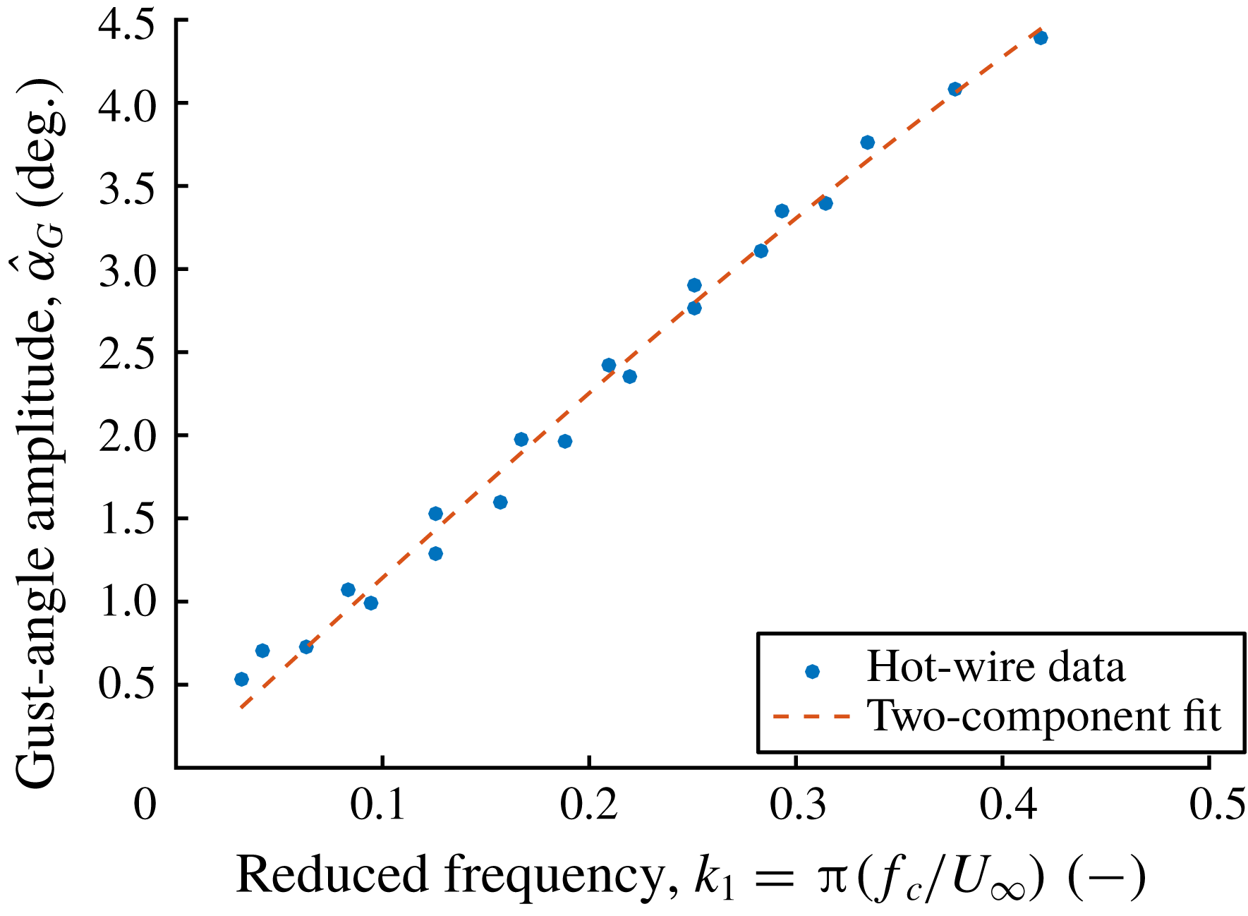
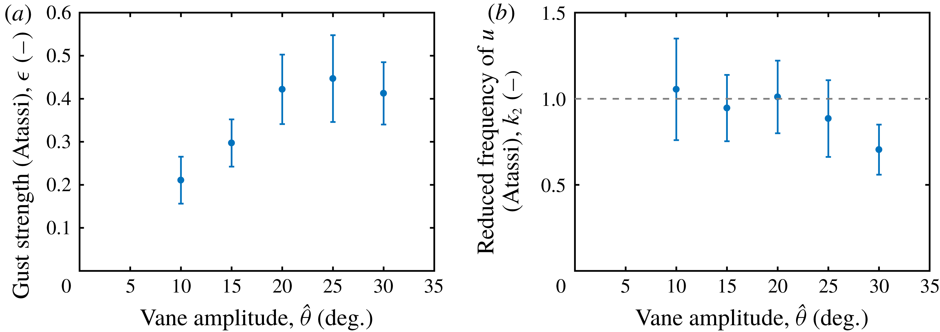
Additionally, for the data sets taken behind the nine-vane grid configuration, a two-parameter nonlinear regression fit based on (2.5) was employed to model the data. Through this type of fit, estimates for $\unicode[STIX]{x1D716}$ and $k_{2}$ were computed. As shown in figures 8(a) and 8(b), between $\hat{\unicode[STIX]{x1D703}}=10^{\circ }$ and $\hat{\unicode[STIX]{x1D703}}=25^{\circ }$ , $\unicode[STIX]{x1D716}$ increased linearly with $\hat{\unicode[STIX]{x1D703}}$ , and $k_{2}$ remained approximately constant within confidence intervals. From $\hat{\unicode[STIX]{x1D703}}=25^{\circ }$ on, the effects of full stall on the grid vanes caused these trends to break down. For the nine-vane grid configuration, the grid amplitude could be correlated to the Atassi definition of gust strength as long as stall effects were not considerable. More importantly, the data provided an estimate for $k_{2}$ – the distinguishing factor between the Sears and Atassi theories – that remained at a constant non-zero value across the range of grid amplitudes employed in the experiments. The average of the estimates below $\hat{\unicode[STIX]{x1D703}}=25^{\circ }$ , $k_{2}=1.0$ , was used to compute Atassi function values for all experiments using the nine-vane grid configuration, since most of the amplitudes used in this study were within the range $5^{\circ }<\hat{\unicode[STIX]{x1D703}}<25^{\circ }$ .

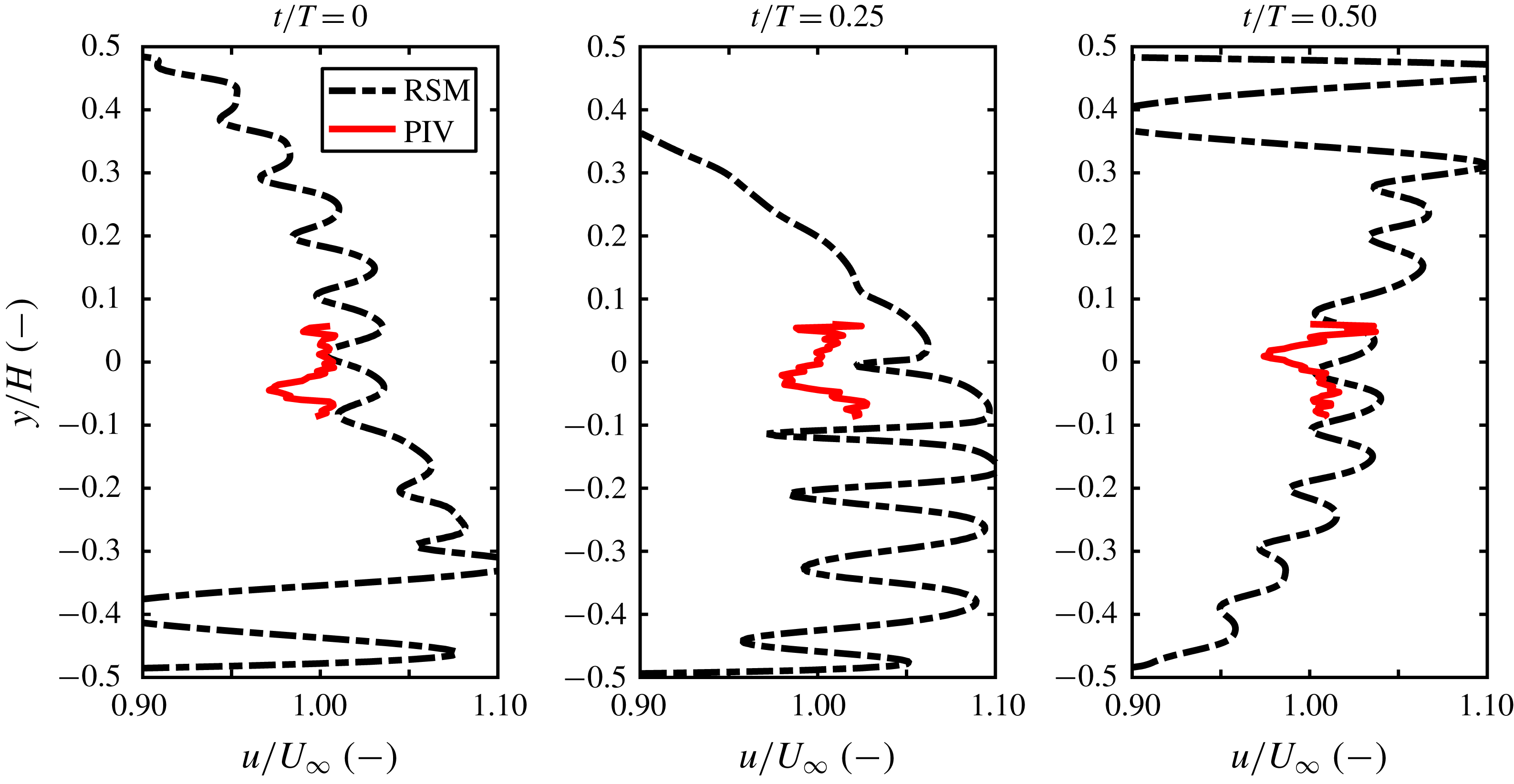
These results were confirmed in experiments and simulations of the active grid without the test airfoil installed. The $u$ component of the flow velocity is shown to fluctuate significantly in time and across the height of the wind tunnel in figure 9, which compares PIV data taken in experiments with data from corresponding numerical simulations. The experimental data were limited in scope by the width of the laser sheet, whereas the simulations resolved the entire cross-section of the wind tunnel. The numerical results suggest further that the likely cause of these fluctuations lies in the combination of the wake profiles of the vanes in the centre region of the tunnel and the use of focused protocols, which are responsible for the large-scale undulations in velocity across the height of the tunnel. These results confirmed that the value of $k_{2}$ for the Atassi function is significantly greater than zero for the nine-vane configuration.

Figure 7.

Two-parameter fit (based on (2.5)) of hot-wire data taken behind the nine-vane active-grid configuration at the location of the leading edge of the test airfoil, for ten grid frequencies and three free-stream velocities. The grid vanes oscillated through $\hat{\unicode[STIX]{x1D703}}=10^{\circ }$ .

Figure 8.

Estimated values for the parameters $k_{2}$ and $\unicode[STIX]{x1D716}$ for various vane amplitudes in the grid’s nine-vane configuration, computed using the type of fit shown in figure 7. At most vane amplitudes, $\unicode[STIX]{x1D716}$ increased monotonically and $k_{2}$ remained relatively constant. The value of $k_{2}$ used in these experiments is represented as a dashed line.

Figure 9.

Variation of the normalized velocity fluctuations in $u$ across the height of the wind tunnel with the active grid running a focused protocol in its nine-vane configuration, from simulations and experiments. The plots represent different dimensionless time instants $t/T$ within one gust period, and $y/H=0$ represents the location of the leading edge of the airfoil. It is clear that $u$ varies significantly in space and time, implying that $k_{2}$ is non-zero.

5.2 Inflow characterization for the Sears problem

The hot-wire data were also used to determine relationships between $\hat{\unicode[STIX]{x1D6FC}}_{g}$ and $\hat{\unicode[STIX]{x1D703}}$ for the six-vane grid configuration. Since the goal of using this grid configuration was to achieve $k_{2}\approx 0$ , it was not necessary to estimate $k_{2}$ and $\unicode[STIX]{x1D716}$ using the two-parameter fits discussed above. 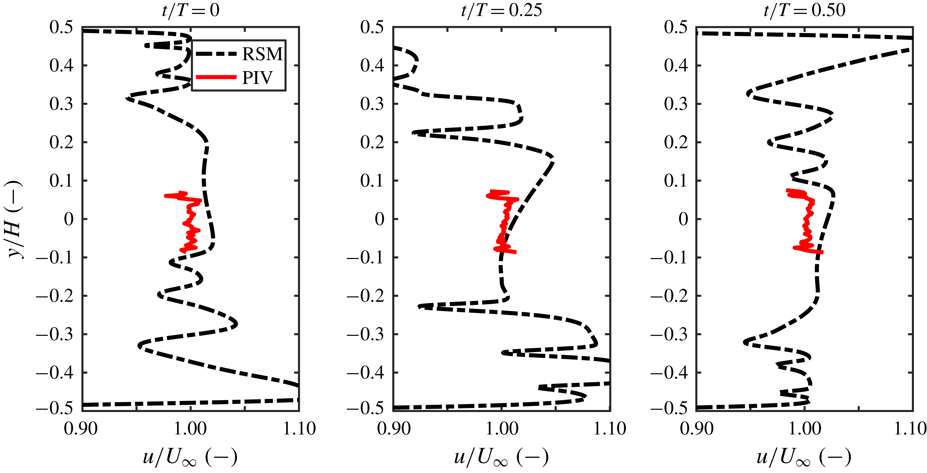Thus, the fluctuations in the $u$ -component of the flow velocity were observed as an indicator of the presence of a significant $k_{2}$ -fluctuation in the same manner as described in the section above. To this end, results from both stereo PIV experiments in the empty tunnel and numerical simulations of the set-up were compared. Figures 10 and 11 show the experimental and simulated properties of the flow field from grid motions at $f=10~\text{Hz}$ , $U_{\infty }=15~\text{m}~\text{s}^{-1}$ and $\hat{\unicode[STIX]{x1D703}}=11.73^{\circ }$ . The $u$ -profile across the height of the tunnel, shown in figure 10, remained relatively uniform across the central region of the tunnel in both simulations and experiments, with no evidence of the temporal and spatial fluctuations present in figure 9 that signified a non-zero $k_{2}$ . 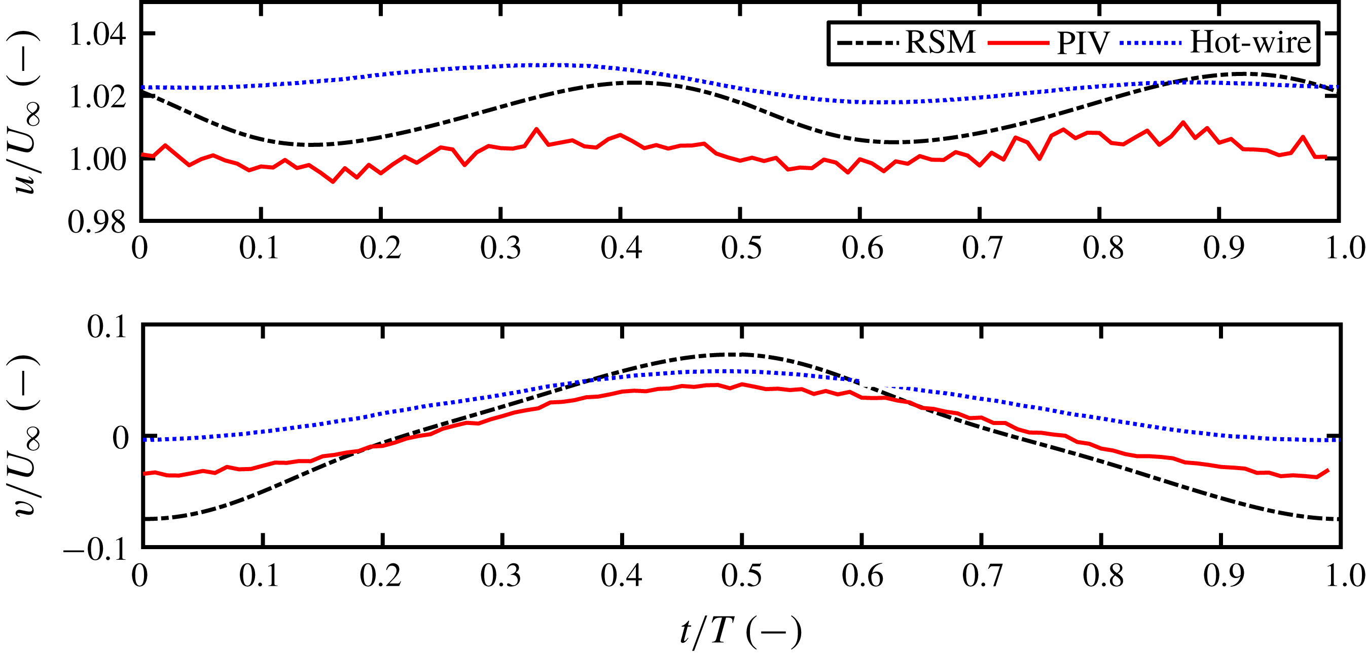Additionally, the fluctuations of $u$ in time were very small (of the order of 1 % of $U_{\infty }$ ), further suggesting that $k_{2}$ for the six-vane grid configuration was effectively zero. The fact that the PIV data and data from the numerical simulations exhibited such strong agreement suggests that the simulations can be used reliably to characterize the inflow conditions in the tunnel in the region of the test airfoil.

Figure 10.

Variation of the normalized velocity fluctuations in $u$ across the height of the wind tunnel with the active grid running a limited protocol in its six-vane configuration, from simulations and experiments. Three dimensionless time instants $t/T$ within one gust period are given. Here, $u$ remains effectively constant in the region of the test airfoil, implying $k_{2}=0$ .

Figure 11.

Evolution of the normalized velocity fluctuations in $u$ and $v$ over a single gust period with the six-vane configuration and limited protocols, from simulations and experiments (PIV and hot-wire probe data). The data agree remarkably well in magnitude and trend, showing that the variations in $u$ are small and thus that $k_{2}\approx 0$ .

5.3 Measurements of the Sears problem

After the flows produced by the active grid had been characterized, the two grid configurations were used to investigate the Sears and Atassi functions in their respective flow situations. The Sears function was tested using the six-vane grid configuration and limited grid protocols. Tests were conducted using two free-stream velocities of $U_{\infty }=15$ and $20~\text{m}~\text{s}^{-1}$ (corresponding to Reynolds numbers of $200\,000$ and $260\,000$ ) over a range of gust frequencies, with vane amplitudes tuned to produce gusts with $\hat{\unicode[STIX]{x1D6FC}}_{g}=2^{\circ }$ . 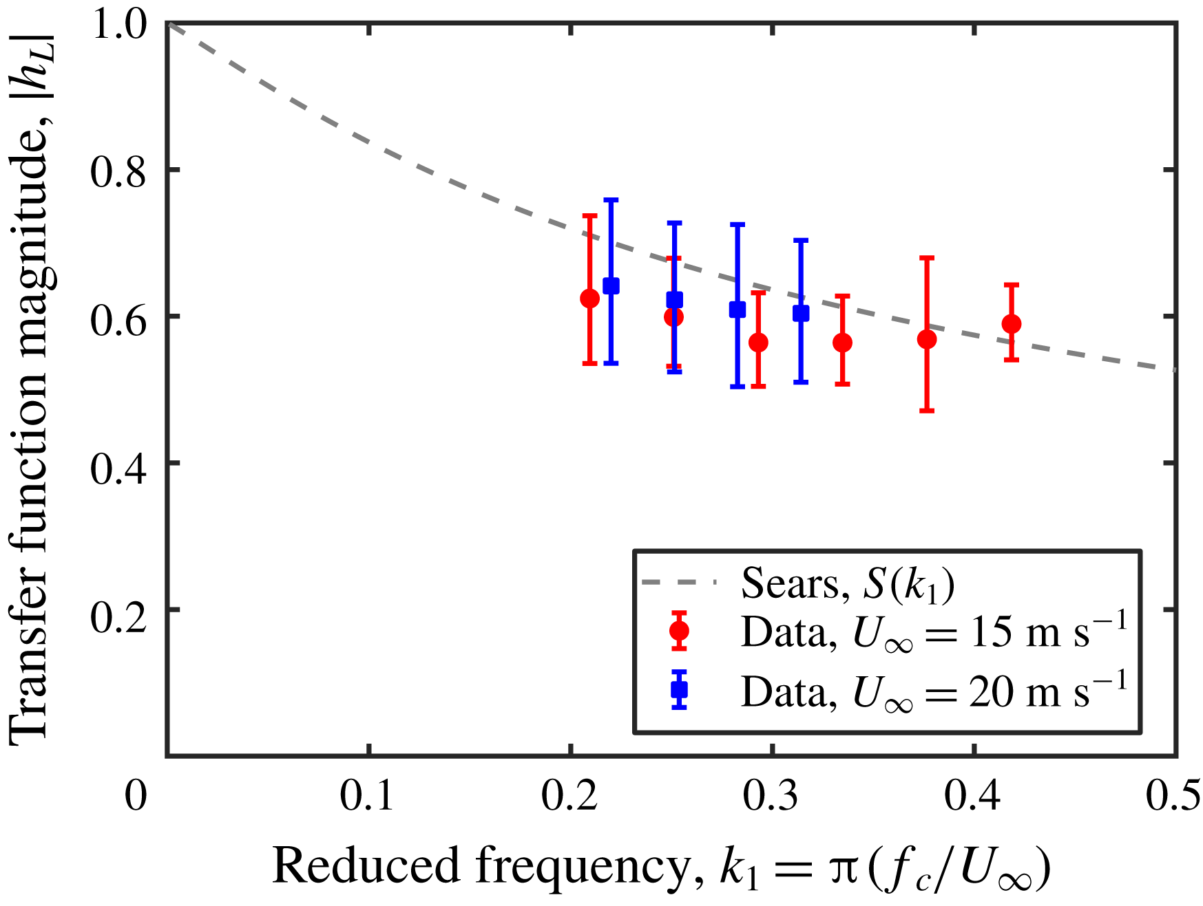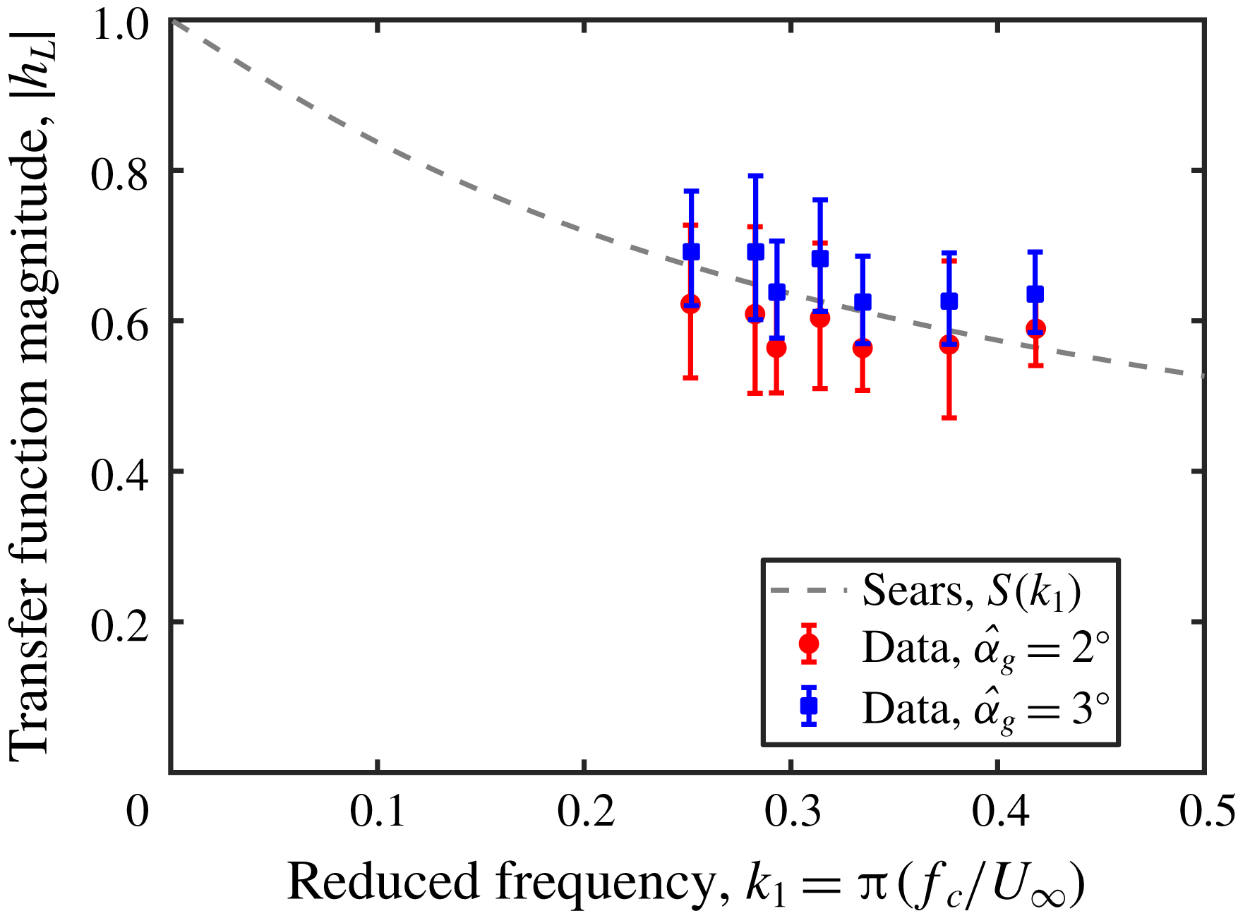This amplitude was chosen to avoid dynamic effects and flow separation on the thin airfoil while maintaining a high enough signal-to-noise ratio from the force balances. The experimental data from this investigation are shown in figure 12. These data follow the trend of the Sears function reasonably well within one standard error.

To verify that $\hat{\unicode[STIX]{x1D6FC}}_{g}$ does not affect experimental correspondence with the Sears function, a series of gusts with $\hat{\unicode[STIX]{x1D6FC}}_{g}=3^{\circ }$ was also tested. These data, shown in figure 13, lie slightly above the $\hat{\unicode[STIX]{x1D6FC}}_{g}=2^{\circ }$ data, likely because of the dynamic effects that would have enhanced the amplitude of the lift fluctuations at this relatively high angle of attack. However, the data still follow the Sears trend within one standard error, thus confirming that the shape of the Sears function holds irrespective of gust strength, as long as flow separation does not occur. Values of $\hat{\unicode[STIX]{x1D6FC}}_{g}$ smaller than $2^{\circ }$ were also tested, but these did not exhibit a clear trend due to the influence of noise.

Figure 12.

Gust response of a NACA 0006 airfoil under Sears inflow conditions for a variation of the reduced frequency $k_{1}$ and a gust-angle amplitude of $\hat{\unicode[STIX]{x1D6FC}}_{g}=2^{\circ }$ . Aside from the single outlier, the data follow the general trend of the Sears function.

Figure 13.

Gust response of a NACA 0006 airfoil under Sears inflow conditions for a variation of the reduced frequency $k_{1}$ . Two gust-angle amplitudes ( $\hat{\unicode[STIX]{x1D6FC}}_{g}=2^{\circ }$ and $\hat{\unicode[STIX]{x1D6FC}}_{g}=3^{\circ }$ ) are shown. As predicted by the theory, there is little difference between the two cases. The slight offset in the $3^{\circ }$ case could be due to the onset of dynamic-stall effects on the thin airfoil.

In order to improve the convergence of the experimental data onto the Sears function, further measures were taken to ensure that the experimental flow conditions conformed to the stipulations of the Sears problem. Because of the thin profile of the NACA 0006 airfoil, flow separation was predicted by XFOIL to occur on the airfoil even at low angles of attack. To hinder these deviations from the theory, thin strips of tape were applied to the airfoil in order to trip transition to turbulence in the boundary layer. The strips of tripping tape used were 3.5 mm wide and 0.1 mm thick, and were placed symmetrically on both sides of the airfoil. Three separate locations along the chord of the airfoil were tested: $x=0.05c$ , $0.10c$ , and $0.40c$ . Static lift-drag measurements at zero angle of attack showed an increase in the total drag over the case of the airfoil without tape for free-stream velocities between 10 and $25~\text{m}~\text{s}^{-1}$ , implying higher skin friction on the airfoil’s surfaces due to turbulence in the boundary layer. Additionally, the linear regime of the lift slope was extended when tape was present, especially at higher free-stream velocities. These observations strongly suggested that the tripping tape was effective in inducing transition to turbulence in the boundary layers on the airfoil.

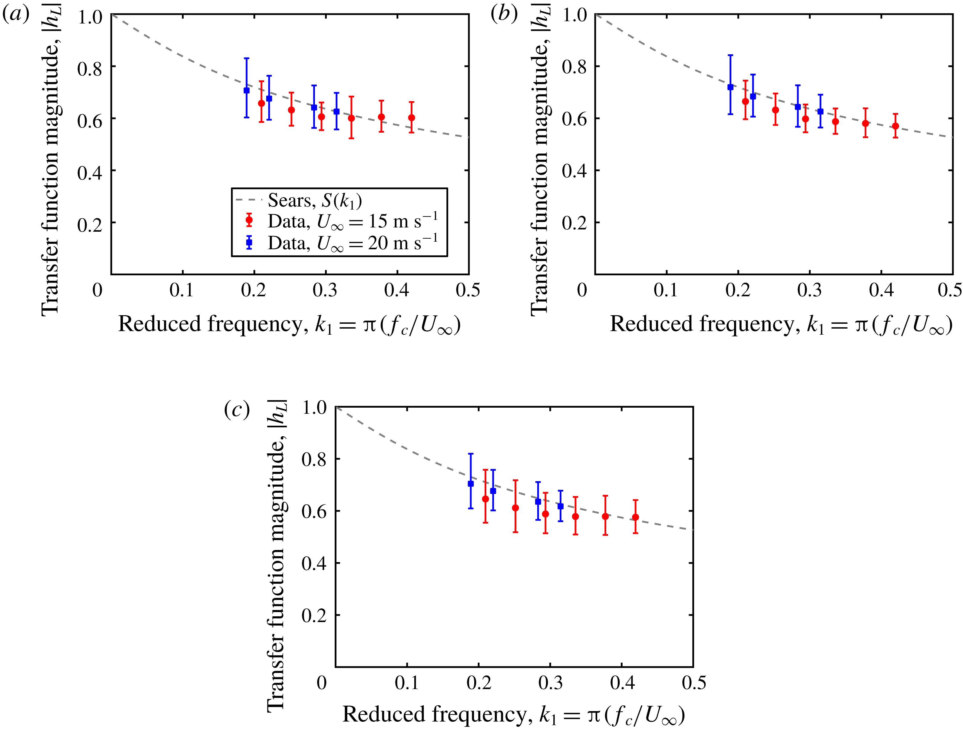
Each of the three tape locations was tested over the set of reduced frequencies and free-stream velocities from the original Sears function series. The data from these series of experiments are shown in figure 14(a–c). In all three cases, the correspondence with the Sears function is significantly improved compared to the case without tape given in figure 12. This result itself confirms in retrospect that the tripping tape did indeed affect the character of the boundary layer, as all other experimental parameters remained the same between the series. The degree of correspondence can be quantified by comparing the mean square error between each data set and the Sears function: for the tape locations of $x=0.05c$ , $0.10c$ and $0.40c$ , the mean square errors were $8.79\times 10^{-4}$ , $6.62\times 10^{-4}$ and $1.36\times 10^{-3}$ . These values are significantly lower than the case without tripping tape, which had a mean square error of $3.04\times 10^{-3}$ . The best convergence was observed in the case where the tripping tape was located nearest to the point of greatest curvature on the airfoil.

Figure 14.

Gust response of a NACA 0006 airfoil under Sears inflow conditions for a variation of the reduced frequency $k_{1}$ at $\hat{\unicode[STIX]{x1D6FC}}_{g}=2^{\circ }$ , with the addition of tripping tape at (a) 5 %, (b) 10 % and (c) 40 % of the chord length behind the leading edge. The convergence to the Sears function was significantly improved from the clean airfoil configuration, with the best agreement observed in case (b).

Jancauskas and Melbourne speculated that the physical cause of the improved convergence with increasing turbulence intensity lay in the fact that turbulent flows generally follow the shapes of profiles better than laminar flows. According to this line of reasoning, flows with high levels of background turbulence would reduce separation and boundary-layer thickness effects, thereby making the overall flow field fit the assumptions of Sears more closely. The ambiguity with their experiments, however, was that the incoming gusts themselves were turbulent, and therefore the root cause of the effect could not be localized to the surface of the test profile itself. In this study, the gusts produced had very low levels of background turbulence, and therefore the cause of the improved convergence could be isolated to the surface of the airfoil. The character of the boundary layer on the airfoil is thus a critical parameter for determining how well the Sears function matches experimental data. The mechanism by which this occurs remains unclear. The hypothesis of Jancauskas and Melbourne is still a feasible explanation; another explanation could stem from the argument that the transport of momentum from the gust to the airfoil is more effective in turbulent rather than laminar boundary layers. The latter hypothesis would explain why no clear trend was found when gusts with $\hat{\unicode[STIX]{x1D6FC}}_{g}=1^{\circ }$ were used. In either case, the results presented here demonstrate that the presence of turbulent boundary layers on an airfoil leads to better correspondence with the Sears function. This finding is rather counterintuitive in light of the potential-flow assumptions of the Sears theory, and suggests that the Sears function may be far more applicable in real-world flow situations than its first-order origins would make it appear. This particular hypothesis will be addressed in future studies.

5.4 Measurements of the Atassi problem

In order to validate the Atassi function in experiments, the nine-vane grid configuration was employed. As for the Sears function, an initial range of reduced frequencies was tested with a constant gust-angle amplitude of $\hat{\unicode[STIX]{x1D6FC}}_{g}=2^{\circ }$ . It has been shown that though the Atassi function is normalized by the gust-strength parameter $\unicode[STIX]{x1D716}$ , multiplying the function by the adjustment factor $|k|/k_{1}$ is equivalent to normalizing the function by $\hat{\unicode[STIX]{x1D6FC}}_{g}$ . 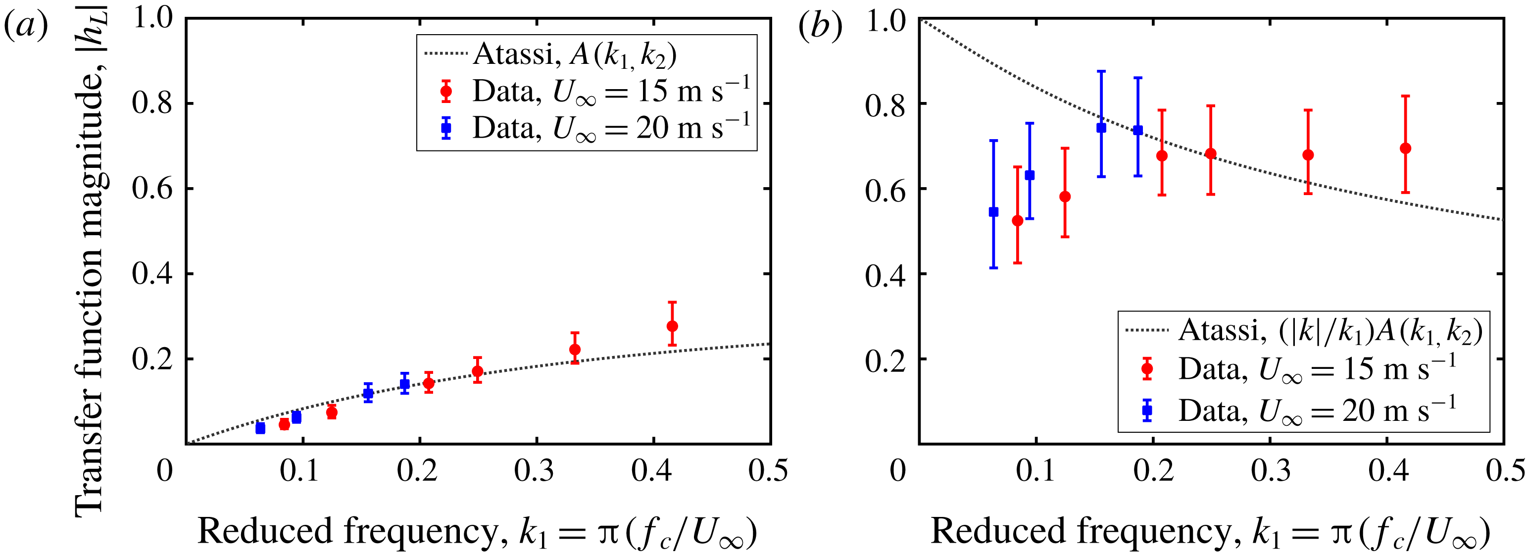To demonstrate this fact experimentally, the same set of data is shown in figures 15(a) and 15(b), normalized by $\unicode[STIX]{x1D716}$ and $\hat{\unicode[STIX]{x1D6FC}}_{g}$ and compared against $A(k_{1},k_{2})$ and $(|k|/k_{1})A(k_{1},k_{2})$ , respectively. For the former case, the value of $k_{2}$ was fixed at $k_{2}=1$ , taken from the analysis of the hot-wire probe data detailed previously. Under both normalizations, the data generally follow the theoretical predictions within error for $k_{1}>0.15$ . The difference in the sizes of the error bars is due to the differences in the magnitudes of the values of the transfer function. The error bounds are significantly larger than those observed in equivalent Sears-function experiments. Furthermore, what appear to be slight deviations from $A(k_{1},k_{2})$ for $k_{1}<0.15$ are shown to be significant departures from the adjusted function $(|k|/k_{1})A(k_{1},k_{2})$ . The reason for these departures will be discussed below. For the purposes of comparison with the Sears function, the data presented in all subsequent plots will be normalized by $\hat{\unicode[STIX]{x1D6FC}}_{g}$ and plotted with the adjusted Atassi function.

Figure 15.

Gust response of a NACA 0006 airfoil under Atassi inflow conditions for a variation of the reduced frequency $k_{1}$ with $k_{2}=1$ and $\hat{\unicode[STIX]{x1D6FC}}_{g}=2^{\circ }$ , with the data normalized by the gust strengths $\unicode[STIX]{x1D716}$ (a) and $\hat{\unicode[STIX]{x1D6FC}}_{g}$ (b). Reasonable agreement with theory is observed for $k_{1}\gtrsim 0.15$ .

Since the Atassi function, like the Sears function, does not depend on the gust strength, changes in the gust-strength parameters $\unicode[STIX]{x1D716}$ and $\hat{\unicode[STIX]{x1D6FC}}_{g}$ should not affect the trends observed in the properly normalized experimental data. Since these parameters are related through (2.5), either one can be held constant over a given range of reduced frequencies by setting the vane amplitude $\hat{\unicode[STIX]{x1D703}}$ of the active grid accordingly. As outlined for the six-vane grid configuration used to validate the Sears function, changing $\hat{\unicode[STIX]{x1D703}}$ allows $\hat{\unicode[STIX]{x1D6FC}}_{g}$ to be controlled for a given value of $k_{1}$ . $\unicode[STIX]{x1D716}$ , on the other hand, scales proportionally with $\hat{\unicode[STIX]{x1D703}}$ without depending on $k_{1}$ (cf. figure 8 a), thus implying that a constant $\hat{\unicode[STIX]{x1D703}}$ yields a constant value of $\unicode[STIX]{x1D716}$ irrespective of $k_{1}$ and $\hat{\unicode[STIX]{x1D6FC}}_{g}$ . The latter variant was employed by Cordes et al. (Reference Cordes, Kampers, Meißner, Tropea, Peinke and Hölling2017) using the older, three-dimensional configuration of the Oldenburg active grid.

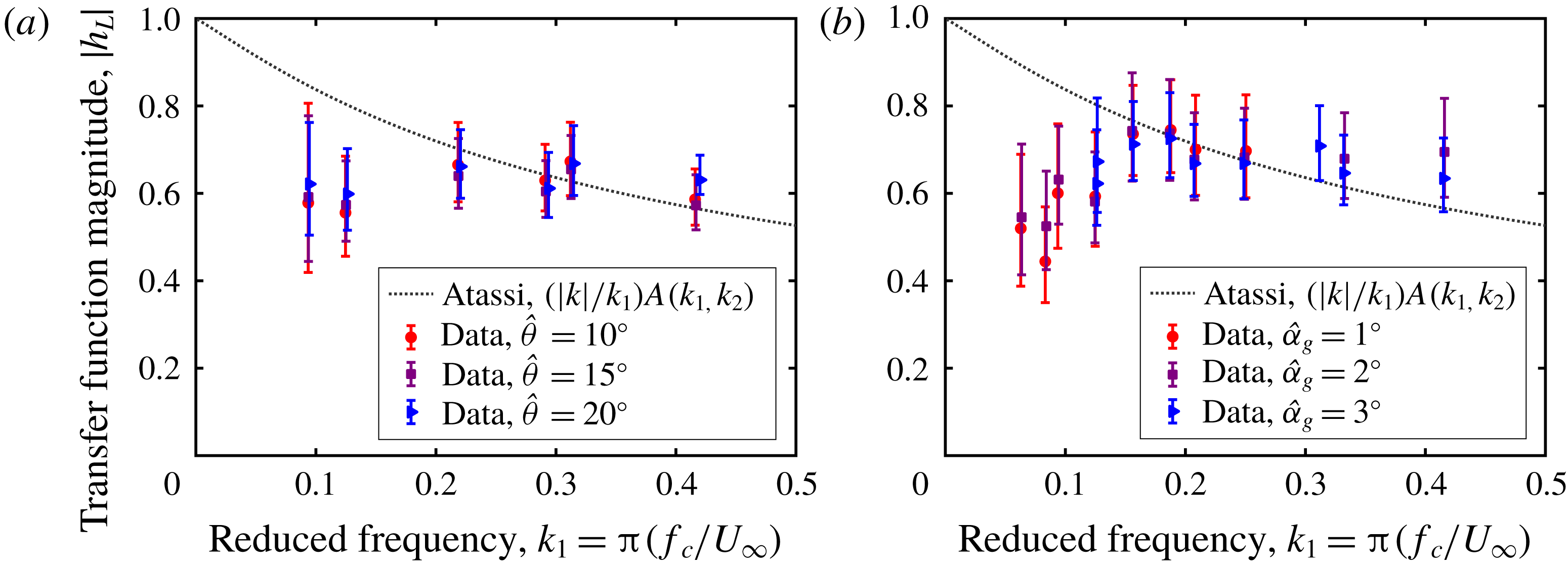
A range of grid amplitudes and gust-angle amplitudes was therefore tested in order to demonstrate that the Atassi function is independent of both $\hat{\unicode[STIX]{x1D6FC}}_{g}$ and $\unicode[STIX]{x1D716}$ . The results for $10^{\circ }\leqslant \hat{\unicode[STIX]{x1D703}}\leqslant 20^{\circ }$ and $1^{\circ }\leqslant \hat{\unicode[STIX]{x1D6FC}}_{g}\leqslant 3^{\circ }$ are shown in figures 16(a) and 16(b), respectively. As expected, the trend of the data remained unchanged, including the deviation of the data from theoretical predictions for $k_{1}<0.15$ . This confirmed that both definitions of gust strength worked in practice to collapse the data, further supporting the idea that the Atassi function is simply an extension of the Sears function.

Figure 16.

Gust response of a NACA 0006 airfoil under Atassi inflow conditions for a variation of the reduced frequency $k_{1}$ , across variations in (a) the vane amplitude $\hat{\unicode[STIX]{x1D703}}$ and (b) the gust-angle amplitude $\hat{\unicode[STIX]{x1D6FC}}_{g}$ . In both cases, the data follow the trend of the Atassi function for $k_{1}\gtrsim 0.15$ .

Numerical simulations of a similar problem confirmed these results. These simulations were carried out to model the experiment of Cordes et al. (Reference Cordes, Kampers, Meißner, Tropea, Peinke and Hölling2017), which had obtained a general Atassi trend despite the use of an incorrect normalization. A Clark-Y profile (11.7 % thickness) with a chord length of $c=0.18~\text{m}$ and at zero angle of attack was used as the test airfoil, and two-dimensional RSM simulations were carried out at three free-stream velocities and a range of grid frequencies. The grid was modelled with focused protocols and amplitudes of $\hat{\unicode[STIX]{x1D703}}=30^{\circ }$ , thus producing gusts with non-negligible fluctuations in $u$ . 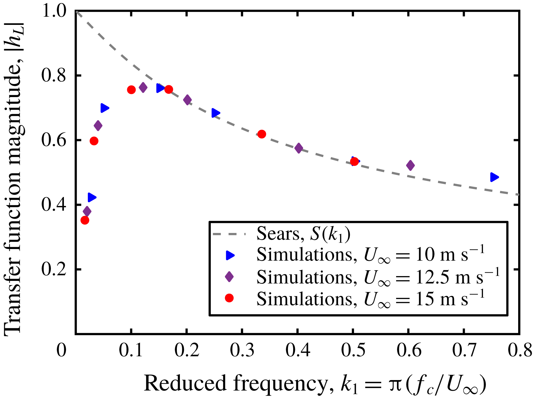The forces on the airfoil were computed from the flow field. More information regarding the set-up of these simulations is given in Wegt (Reference Wegt2017), and the resulting transfer-function values are shown in figure 17. In spite of the use of different airfoil profiles, the same trend as that observed in the experiments detailed above was retrieved in the numerical data. Most strikingly, the deviation from the Sears and adjusted Atassi functions occurred in the simulations at around the same reduced frequency of $k_{1}\approx 0.15$ .

Figure 17.

Two-dimensional RSM simulations of the set-up of Cordes et al. (Reference Cordes, Kampers, Meißner, Tropea, Peinke and Hölling2017) with a Clark-Y airfoil and using a nine-vane active-grid configuration. Despite the use of a different type of airfoil, there is very good agreement between these simulations and the experiments shown in figure 16(a,b).

All of the data presented thus far align well with the Atassi function for $k_{1}>0.15$ , but deviate from theoretical predictions for $k_{1}<0.15$ . This deviation is systematic across the range of free-stream velocities, grid frequencies and gust strengths $\hat{\unicode[STIX]{x1D6FC}}_{g}$ and $\unicode[STIX]{x1D716}$ tested in these experiments, and will be shown in the next section to be a consequence of the experimental apparatus and not of any failings of the theory of Atassi. The data for $k_{1}>0.15$ for both the Sears and Atassi functions demonstrate quite clearly that the adjusted Atassi function is identical to the Sears function irrespective of the value of $k_{2}$ . This confirms the analysis of the two models presented in § 2, and suggests that the Sears function can be used to model the behaviour of a thin symmetric airfoil subjected to streamwise and normal gusts at zero mean angle of attack. Mathematically, this is not a novel result. The experiments presented here, however, provide a helpful framework for past and future experimental investigations. For example, these observations offer an explanation for the trends seen in previous experiments involving gusts generated by a turbulence grid (e.g. Larose Reference Larose1999; Hatanaka & Tanaka Reference Hatanaka and Tanaka2002; Lysak et al. Reference Lysak, Capone and Jonson2016). The gusts in these studies would have had significant $k_{2}$ gust components, and therefore would have been better represented by the Atassi function. However, since all of these data were normalized by the Sears gust strength $\hat{\unicode[STIX]{x1D6FC}}_{g}$ instead of the Atassi gust strength $\unicode[STIX]{x1D716}$ , each was able to retrieve a clear Sears trend.

5.5 Influence of inflow turbulence level

It has been noted that the convergence of the data around the Atassi function appears to be worse than that observed in the Sears function experiments, and that the data fail to follow the Atassi function for $k_{1}<0.15$ . These idiosyncrasies are effects of the turbulent wakes of the central vanes in the nine-vane grid configuration.

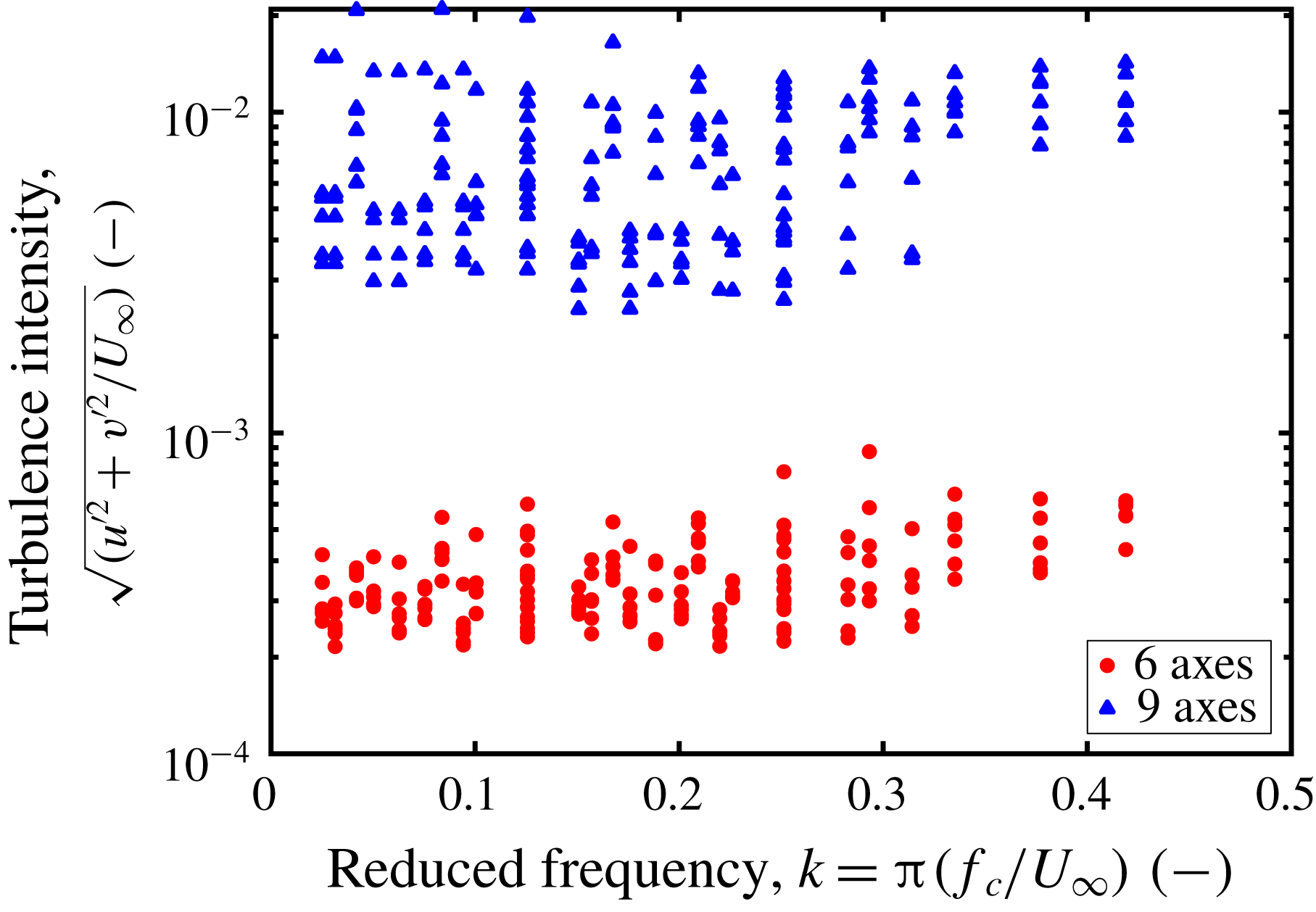
Jancauskas & Melbourne (Reference Jancauskas and Melbourne1983) showed that increasing the background turbulence intensity in gusty flows on bridge-deck sections leads to better correspondence with the Sears function. In the nine-vane grid configuration, the wakes of the central vanes were responsible for higher turbulence intensities in the flows impinging on the airfoil than in the six-vane grid configuration where the middle section of the tunnel was free from disturbances. This was determined using the hot-wire probe data from the tunnel characterization experiments. A centred moving average over 200 data samples was applied to each velocity component in order to extract the turbulent velocity fluctuations from the generally sinusoidal velocity profile of the gust. A turbulence intensity was then computed from these two velocity fluctuation components for every combination of $k_{1}$ and $\hat{\unicode[STIX]{x1D703}}$ tested. The distribution of these turbulence intensity values is represented in figure 18. From these data, it is clear that the central three axes in the nine-vane grid configuration generated uniformly higher background turbulence levels than were observed in the six-vane grid configuration.

Figure 18.

Turbulence intensities of the fluctuation velocities from the six- and nine-vane grid configurations, computed from hot-wire measurements at the position of the leading edge of the test airfoil. The turbulence intensities behind the nine-vane grid were consistently higher than those behind the six-vane grid.

One would expect, then, that the Atassi data would converge to the theoretical predictions more cleanly than the Sears data. This, however, was not the case. Here, it is necessary to distinguish between background turbulence and turbulent fluctuations within the gust itself. The experimental apparatus of Jancauskas and Melbourne used a turbulence-generating screen to produce nominally homogeneous turbulence, on top of which a fluctuating velocity signal was overlaid by their gust-generation apparatus. In the present study, by contrast, the source of the turbulence intensity was the wakes of the central vanes of the active grid. The test airfoil would pass in and out of these turbulent wakes, leading to alternating smooth and turbulent flow conditions within a single gust period. This intermittent turbulent effect was not captured by the values of $\hat{\unicode[STIX]{x1D6FC}}_{g}$ used to normalize the experimental data, since these were computed from phase-averaged velocity signals. To quantify the extent of this effect, in addition to computing the gust-angle amplitude from the phase-averaged velocity signals, the peak velocity values within each gust period were isolated, and an average amplitude and corresponding angle of attack, $\hat{\unicode[STIX]{x1D6FC}}_{peak}$ , was computed from these local maxima. 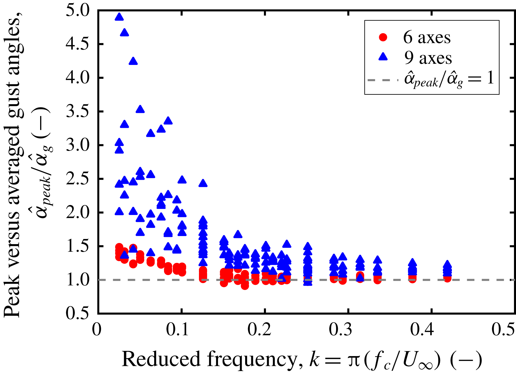The ratio of $\hat{\unicode[STIX]{x1D6FC}}_{peak}$ to $\hat{\unicode[STIX]{x1D6FC}}_{g}$ for a range of grid protocols with $10^{\circ }\leqslant \hat{\unicode[STIX]{x1D703}}\leqslant 30^{\circ }$ is plotted in figure 19. The plot shows that the peak velocity fluctuations were significantly larger than unity for $k_{1}\lesssim 0.15$ , and remained close to unity for $k_{1}\gtrsim 0.15$ . These results demonstrate that the intermittent turbulent fluctuations caused by the wakes of the central vanes had a significant effect on the quality of the gusts produced by the active grid precisely in the reduced frequency regime in which a deviation from theory was observed in the data. The large instantaneous angles of attack from the turbulence in the gust, combined with the high frequencies of these forcings, contributed to a diminished gust response of the airfoil in this regime. These turbulent peaks were much less significant for $k_{1}\gtrsim 0.15$ , implying that the data for these higher reduced frequencies are free from the influence of the vane wakes. Preliminary simulations using oscillating inflow conditions instead of simulated vanes to produce gusts confirmed that data at low reduced frequencies follow the Sears and adjusted-Atassi trend when the influence of the grid is removed (cf. Wegt Reference Wegt2017).

The effect of turbulence on the gust response of airfoils thus depends heavily on the character of the turbulence in question. Jancauskas & Melbourne (Reference Jancauskas and Melbourne1983) showed that homogeneous background turbulence can improve correspondence with the Sears function. The experiments with tripping tape presented in this work have demonstrated that inducing turbulence in the boundary layer of an airfoil can similarly improve convergence. This suggests that small-scale homogeneous turbulence enhances the ability of the flow to interact with the airfoil, by facilitating momentum transport through the boundary layer or by hindering separation on surfaces with an adverse pressure gradient. Large-scale intermittent turbulent fluctuations, on the other hand, have been shown to increase experimental uncertainty and cause significant deviations from theoretical predictions at low reduced frequencies. Because these turbulent fluctuations are large in magnitude and frequency content compared to the baseline sinusoidal gust signal, reconciling their effects with the predictions of the Sears and Atassi functions is a non-trivial problem that lies beyond the scope of this work. This problem, however, is similar to the interaction of an airfoil with a periodic vortical gust disturbance, and could be of interest to several applications in aerodynamics, such as formation flight in flocks.

Figure 19.

The ratio of peak gust-angle amplitude $\hat{\unicode[STIX]{x1D6FC}}_{peak}$ to phase-averaged gust-angle amplitude $\hat{\unicode[STIX]{x1D6FC}}_{g}$ from the six- and nine-vane grid configurations, computed from hot-wire measurements. Values of $(\hat{\unicode[STIX]{x1D6FC}}_{peak}/\hat{\unicode[STIX]{x1D6FC}}_{g})\gtrsim 2$ represent a strong influence of the wakes of the central vanes on the character of the gust.