1. Introduction
Swimming micro-organisms are ubiquitous in nature in the form of biological cells. Examples of biological swimmers that have been studied experimentally include bacteria (Porter Reference Porter1976; Berg Reference Berg2004), algae (Polin et al. Reference Polin, Tuval, Drescher, Gollub and Goldstein2009; Witman Reference Witman2009) and spermatozoa (Suarez & Pacey Reference Suarez and Pacey2006). More recently it has been possible to fabricate artificial micro-swimmers such as catalytic nanorods (Paxton et al. Reference Paxton, Kistler, Olmeda, Sen, St. Angelo, Cao, Mallouk, Lammert and Crespi2004), a three-sphere swimmer realised with optical tweezers (Najafi & Golestanian Reference Najafi and Golestanian2004; Leoni et al. Reference Leoni, Kotar, Bassetti, Cicuta and Lagomarsino2009), or a chain of colloidal magnetic particles (Dreyfus et al. Reference Dreyfus, Baudry, Roper, Fermigier, Stone and Bibette2005). Interest in the propulsion and behaviour of micro-swimmers has lead to extensive early theoretical work (Taylor Reference Taylor1951; Lighthill Reference Lighthill1952; Hancock Reference Hancock1953; Gray & Hancock Reference Gray and Hancock1955; Blake Reference Blake1971b ; Purcell Reference Purcell1977; Lauga & Powers Reference Lauga and Powers2009) and more recently a number of theoretical models of swimmers have also proved useful in helping to understand their motility (Avron, Kenneth & Oaknin Reference Avron, Kenneth and Oaknin2005; Ishikawa, Simmonds & Pedley Reference Ishikawa, Simmonds and Pedley2006; Tam & Hosoi Reference Tam and Hosoi2007; Alexander & Yeomans Reference Alexander and Yeomans2008; Golestanian & Ajdari Reference Golestanian and Ajdari2008).
Because of their size, micro-organisms swim at low Reynolds number,
 $\mathit{Re}\approx 10^{-4}$
(Purcell Reference Purcell1977). Hence the fluid motion is governed by the Stokes equations. As micro-organisms move they set up velocity fields which stir the surrounding fluid. Recently, these flow fields have been measured experimentally in a bulk fluid and near a solid surface (Drescher et al.
Reference Drescher, Goldstein, Michel, Polin and Tuval2010, Reference Drescher, Dunkel, Cisneros, Ganguly and Goldstein2011).
The displacement of tracer particles in the flow leads to enhanced diffusion, or stirring. This is thought to confer a biological advantage by increasing nutrient supply (Sokolov et al. Reference Sokolov, Goldstein, Feldchtein and Aranson2009; Katija Reference Katija2012; Jepson et al. Reference Jepson, Martinez, Schwarz-Linek, Morozov and Poon2013), and may have an application to enhancement of mixing in microfluidic channels (Kim & Breuer Reference Kim and Breuer2007). Stirring was first measured experimentally in concentrated suspensions (Wu & Libchaber Reference Wu and Libchaber2000) and later in dilute suspensions in various geometries (Leptos et al. Reference Leptos, Guasto, Gollub, Pesci and Goldstein2009; Kurtuldu et al. Reference Kurtuldu, Guasto, Johnson and Gollub2011; Mino et al. Reference Mino, Mallouk, Darnige, Hoyos, Dauchet, Dunstan, Soto, Wang, Rousselet and Clement2011). Simulations of micro-swimmer suspensions also shows enhanced diffusivities (Underhill, Hernandez-Ortiz & Graham Reference Underhill, Hernandez-Ortiz and Graham2008; Ishikawa, Locsei & Pedley Reference Ishikawa, Locsei and Pedley2010; Thiffeault & Childress Reference Thiffeault and Childress2010; Lin, Thiffeault & Childress Reference Lin, Thiffeault and Childress2011; Thiffeault Reference Thiffeault2014).
To understand enhanced diffusion in a dilute swimmer suspension it is helpful to first consider the motion of a single tracer particle in the flow field of a passing swimmer. Conversely, understanding the features of tracer trajectories obtained in experiments may help the analysis of propulsion and flows created by micro-swimmers. The main purpose of this paper is the analysis of typical tracer trajectories. It has recently been shown that, for a swimmer that moves along an infinite straight trajectory, tracer particles far from the swimmer move in closed loops, whereas those close to the swimmer are entrained by its motion (Darwin Reference Darwin1953; Pushkin, Shum & Yeomans Reference Pushkin, Shum and Yeomans2013). However, in reality bacterial paths are not infinite but often can be approximated by straight lines interspersed with random reorientation phases, called runs and tumbles respectively (Berg & Brown Reference Berg and Brown1972). The effect of random reorientations on tracer diffusion has been considered in Dunkel et al. (Reference Dunkel, Putz, Zaid and Yeomans2010), Miño et al. (Reference Miño, Dunstan, Rousselet, Clément and Soto2013), Pushkin & Yeomans (Reference Pushkin and Yeomans2013) and Morozov & Marenduzzo (Reference Morozov and Marenduzzo2014). Here we will discuss the effect of finite swimmer paths on individual tracer trajectories.
Most experiments on micro-swimmers are performed in finite geometries, such as on microscope slides. Moreover, in biological systems micro-organisms often tend to accumulate near surfaces, as observed experimentally (Rothschild Reference Rothschild1963; Frymier et al. Reference Frymier, Ford, Berg and Cummings1995; Berke et al. Reference Berke, Turner, Berg and Lauga2008; Li & Tang Reference Li and Tang2009; Li et al. Reference Li, Bensson, Nisimova, Munger, Mahautmr, Tang, Maxey and Brun2011; Molaei et al. Reference Molaei, Barry, Stocker and Sheng2014; Vladescu et al. Reference Vladescu, Marsden, Schwarz-Linek, Martinez, Arlt, Morozov, Marenduzzo, Cates and Poon2014) and explained theoretically in terms of long-range hydrodynamic interactions (Berke et al. Reference Berke, Turner, Berg and Lauga2008; Spagnolie & Lauga Reference Spagnolie and Lauga2012) and collisions of cells with the surface (Li et al. Reference Li, Bensson, Nisimova, Munger, Mahautmr, Tang, Maxey and Brun2011). Moreover, interfaces are understood to influence microbial motility, which could lead to the formation of antibiotic-resistant biofilms (Van Loosdrecht et al. Reference Van Loosdrecht, Lyklema, Norde and Zehnder1990; Costerton et al. Reference Costerton, Lewandowski, Caldwell, Korber and Lappin-Scott1995). Therefore, here we extend the research on tracer trajectories near an individual swimmer to the cases where the swimmer is close to a no-slip or free-slip boundary.
In § 2 we summarise the multipole expansion, writing the flow field of a generic micro-swimmer as an expansion in
 $r^{-1}$
, where
 $r$
is the distance from the swimmer. We specialise to the most common physical case of an axisymmetric swimmer, for which many terms of the expansion vanish, and hence obtain a more tractable set of swimmer parameters. This allows us to set up a perturbation theory in
 $r^{-1}$
for the tracer displacement and, using this framework, we obtain the trajectories of tracer particles as a swimmer moves along a straight path of finite length, considering the cases of a boundary absent or present.
We show in particular how a suitable choice of dipolar and quadrupolar coefficients in the multipole expansion can be used to account for flows created by swimmers having finite effective size. Therefore, the multipole expansion can be employed to study features of tracer trajectories both in the far-field and the near-field of micro-swimmers. An example is the entrainment of tracer particles as the swimmer passes close by.
In § 3 we present results for a swimmer in an unbounded fluid. These are based both on numerical solutions of the tracer equation of motion and the perturbation expansion. We compute terms up to sixth order in
 $r^{-1}$
to collect enough information to study the transition from an infinite to a finite swimming path. The tracer paths have a loop-like structure with a size that scales as
 $r^{-1}$
. The loops are almost closed with a final displacement of order
 $r^{-3}$
for an infinite swimming path. For a finite swimming path the loops open up further, giving rise to substantial tracer displacements. We also show that another significant contribution to tracer displacements stems from spiralling of particles about the swimmer axis when micro-swimmers propel by rotating their flagella.
In § 4 we present results for a swimmer moving along a path parallel to a no-slip boundary. We show that even though fluid motion is inhibited near the boundary, tracer particles are pulled along the swimming direction, for pushers and pullers alike, and even more so for swimmers that produce quadrupolar flow fields. Moreover, for swimmers close to the boundary the tracer particles are displaced in the plane perpendicular to the swimming direction, even for non-rotating micro-swimmers. We repeat our calculations for a swimmer near a free-slip boundary, and describe the main similarities and differences.
In § 5 our results are summarised and discussed.
2. Mathematical model
Consider a micro-swimmer moving in the direction
 $\hat{\boldsymbol{e}}_{z}$
along a line a distance
 $H$
above and parallel to a plane boundary located at
 $x=0$
. We assume the swimmer moves with constant velocity
 $V$
so that it is located at position
 $\boldsymbol{R}(t)=(R_{z}^{int}+Vt)\hat{\boldsymbol{e}}_{z}+H\hat{\boldsymbol{e}}_{x}$
at time
 $t$
. We aim to study a tracer particle initially located at position
 $\boldsymbol{r}_{T}^{int}=x_{T}^{int}\hat{\boldsymbol{e}}_{x}+y_{T}^{int}\hat{\boldsymbol{e}}_{y}+z_{T}^{int}\hat{\boldsymbol{e}}_{z}$
at
 $t=0$
, and after time
 $t$
at position
 $\boldsymbol{r}_{T}(t)$
. In the case of a swimmer in an unbounded fluid, in the limit
 $H\rightarrow \infty$
, it is easier to switch to a cylindrical coordinate system so that
 $\boldsymbol{R}(t)=(R_{z}^{int}+Vt)\hat{\boldsymbol{e}}_{z}$
and
 $\boldsymbol{r}_{T}^{int}={\it\rho}_{T}^{int}\hat{\boldsymbol{e}}_{{\it\rho}}+z_{T}^{int}\hat{\boldsymbol{e}}_{z}$
. For brevity, we will write
 ${\it\rho}={\it\rho}_{T}^{int}$
from now onwards.
The tracer displacement is defined as
 ${\rm\Delta}\boldsymbol{r}_{T}(t)=\boldsymbol{r}_{T}(t)-\boldsymbol{r}_{T}^{int}$
, and the final tracer displacement after the swimmer has passed is
 ${\rm\Delta}\boldsymbol{r}_{T}^{\infty }=\lim _{t\rightarrow \infty }{\rm\Delta}\boldsymbol{r}_{T}(t)$
. The relative position vectors of the tracer particle with respect to the swimmer and its image system are written as
 $\boldsymbol{r}=\boldsymbol{r}_{T}^{int}-\boldsymbol{R}(t)$
and
 $\boldsymbol{r}^{\ast }=\boldsymbol{r}_{T}^{int}-\boldsymbol{R}^{\ast }(t)$
respectively, where
 $\boldsymbol{R}^{\ast }=\unicode[STIX]{x1D648}\boldsymbol{R}$
with
 $\unicode[STIX]{x1D648}=\text{diag}(-1,1,1)$
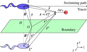
. This geometry is depicted in figure 1.
Geometry diagram for a micro-swimmer moving along a path parallel to a boundary. The unit vector normal to the boundary is
 $\hat{\boldsymbol{n}}=\hat{\boldsymbol{e}}_{x}$
and the swimmer moves at a distance
 $H$
from the boundary with velocity
 $V$
in the
 $z$
direction. Note that the axes are displayed in the bottom-right corner, not at the origin
 $O$
, for clarity.

2.1. Flow field produced by a micro-swimmer
By changing their shape, swimmers exert forces and torques on the fluid they move in. We model these as a distribution of point forces,
 $\boldsymbol{f}({\bf\xi})$
, summed over the swimmer’s surface
 $S$
located at position
 $\boldsymbol{R}+{\bf\xi}$
. The force distribution produces flows around the swimmer
 $$\begin{eqnarray}u_{i}^{sw}(\boldsymbol{r})=\int _{S}f_{j}\unicode[STIX]{x1D611}_{ij}(\boldsymbol{r}-{\bf\xi})\,\text{d}S,\end{eqnarray}$$
where
 $\unicode[STIX]{x1D611}_{ij}(\boldsymbol{r})$
is the appropriate Green’s function of the Stokes equations. For an unbounded fluid, this Green’s function is the Oseen tensor
 $\unicode[STIX]{x1D60E}_{ij}(\boldsymbol{r})=({\it\delta}_{ij}/r+r_{i}r_{j}/r^{3})/(8{\rm\pi}{\it\mu})$
where
 ${\it\delta}_{ij}$
is the Kronecker delta and
 $r=|\boldsymbol{r}|$
. When a no-slip boundary is present, the Green’s function is the Blake tensor (Blake Reference Blake1971a
)
 $$\begin{eqnarray}\unicode[STIX]{x1D609}_{ij}(\boldsymbol{r},\boldsymbol{r}^{\ast })=\unicode[STIX]{x1D60E}_{ij}(\boldsymbol{r})+(-{\it\delta}_{jk}-2H{\it\delta}_{kx}\partial _{j}+H^{2}\unicode[STIX]{x1D614}_{jk}{\rm\nabla}^{2})\unicode[STIX]{x1D60E}_{ik}(\boldsymbol{r}^{\ast }),\end{eqnarray}$$
where
 $H=\boldsymbol{R}\boldsymbol{\cdot }\hat{\boldsymbol{e}}_{x}>0$
and where the derivatives
 $\partial _{j}^{\ast }=\unicode[STIX]{x1D614}_{jl}\partial _{l}$
and
 ${\rm\nabla}^{\ast 2}={\rm\nabla}^{2}$
. For a free-slip interface the Green’s function is
 $\unicode[STIX]{x1D60D}_{ij}(\boldsymbol{r},\boldsymbol{r}^{\ast })=\unicode[STIX]{x1D60E}_{ij}(\boldsymbol{r})+\unicode[STIX]{x1D614}_{jk}\unicode[STIX]{x1D60E}_{ik}(\boldsymbol{r}^{\ast })$
.
We expand (2.1) in a multipole expansion to write the fluid flow generated by a micro-swimmer moving in the
 $z$
direction as
 $$\begin{eqnarray}\boldsymbol{u}^{sw}(\boldsymbol{r};\hat{\boldsymbol{e}}_{z})=\boldsymbol{u}^{D}(\boldsymbol{r},\hat{\boldsymbol{e}}_{z})+\boldsymbol{u}^{Q}(\boldsymbol{r},\hat{\boldsymbol{e}}_{z})+\boldsymbol{u}^{O}(\boldsymbol{r},\hat{\boldsymbol{e}}_{z})+\boldsymbol{u}^{H}(\boldsymbol{r},\hat{\boldsymbol{e}}_{z})+\cdots \,,\end{eqnarray}$$
which contains Stokes dipole
 $\boldsymbol{u}^{D}\sim O(r^{-2})$
, quadrupole
 $\boldsymbol{u}^{Q}\sim O(r^{-3})$
, octupole
 $\boldsymbol{u}^{O}\sim O(r^{-4})$
and higher-order terms. A detailed explanation of the multipole expansion can be found in the work by Jeffrey & Onishi (Reference Jeffrey and Onishi1984) or Kim & Karilla (Reference Kim and Karilla1991, p. 27), or more explicitly in the context of micro-swimmers in the work by Yeomans, Pushkin & Shum (Reference Yeomans, Pushkin and Shum2014).
Many micro-swimmers have, to a good approximation, a shape that is cylindrically symmetric about the swimming direction. This helpfully restricts the number of non-zero components of the swimmer multipole moments. In the supplementary data (available at http://dx.doi.org/10.1017/jfm.2015.269) we compute the residual flow fields in terms of a substantially reduced number of coefficients, the dipole moment
 ${\it\kappa}$
, the quadrupolar moments
 $Q_{\Vert ,\bot ,r}$
, etc., which are experimental observables for a particular individual organism. In the following paragraphs we list the flow fields up to octupolar order, and describe their physical significance.
An autonomous swimmer cannot rely on external forces to move forwards. Therefore there are no Stokeslet terms in (2.3), assuming that the effects of gravity are negligible. This assumption is true for swimmers that are neutrally buoyant, or if their sedimentation velocity is negligible compared to their swimming speed (Ishikawa et al. Reference Ishikawa, Simmonds and Pedley2006). Therefore the leading-order term in (2.3) is the dipolar flow field
 $$\begin{eqnarray}\boldsymbol{u}^{D}(\boldsymbol{r},\hat{\boldsymbol{e}}_{z})=-{\it\kappa}(\hat{\boldsymbol{e}}_{z}\boldsymbol{\cdot }\boldsymbol{{\rm\nabla}})\boldsymbol{u}^{S}(\boldsymbol{r},\hat{\boldsymbol{e}}_{z}),\end{eqnarray}$$
where
 $u_{i}^{S}(\boldsymbol{r},\hat{\boldsymbol{e}}_{j})=\hat{\boldsymbol{e}}_{j}\boldsymbol{\cdot }\unicode[STIX]{x1D611}_{ij}(\boldsymbol{r})$
is the Stokeslet, the flow generated by a point force along
 $\hat{\boldsymbol{e}}_{j}$
, and
 $\partial _{z}=(\hat{\boldsymbol{e}}_{z}\boldsymbol{\cdot }\boldsymbol{{\rm\nabla}})$
is the derivative with respect to the relative position
 $\boldsymbol{r}$
in the swimming direction. The dipolar term describes the balancing forces of propulsion and drag. If
 ${\it\kappa}>0$
the swimmer is known as a pusher, with an extensile flow field (e.g. a sperm cell or Escherichia coli bacterium), where the organism is propelled from behind. If
 ${\it\kappa}<0$
the swimmer is termed a puller, with a contractile flow field (e.g. the Chlamydomonas reinhardtii alga, which performs a breast stroke). The dipole moment
 ${\it\kappa}$
has been measured in experiment and time-averaged for the microphytes Volvox carteri and C. reinhardtii (Drescher et al.
Reference Drescher, Goldstein, Michel, Polin and Tuval2010) and for E. coli (Drescher et al.
Reference Drescher, Dunkel, Cisneros, Ganguly and Goldstein2011).
The quadrupolar flow field of a cylindrically symmetric swimmer can be written as
 $$\begin{eqnarray}\boldsymbol{u}^{Q}(\boldsymbol{r},\hat{\boldsymbol{e}}_{z})=-{\textstyle \frac{1}{2}}(Q_{\Vert }{\rm\nabla}_{\Vert }^{2}+Q_{\bot }{\rm\nabla}_{\bot }^{2}-2Q_{r}\partial _{z}\boldsymbol{{\rm\nabla}}\times )\boldsymbol{u}^{S}(\boldsymbol{r},\hat{\boldsymbol{e}}_{z}),\end{eqnarray}$$
where
 ${\rm\nabla}_{\Vert }^{2}=(\hat{\boldsymbol{e}}_{z}\boldsymbol{\cdot }\boldsymbol{{\rm\nabla}})^{2}$
and
 ${\rm\nabla}_{\bot }^{2}={\rm\nabla}^{2}-{\rm\nabla}_{\Vert }^{2}$
are the Laplace operators parallel to, and in the plane perpendicular to, the swimming direction
 $\hat{\boldsymbol{e}}_{z}$
. The source doublet flow field, a particular combination of the quadrupole terms with
 $Q_{\Vert }=Q_{\bot }$
, allows us to describe the flow around the swimmer’s body, which can help the tracer particles avoid encountering the singularity centre and hence account for the finite size of the cell. This will be discussed further in § 2.2. Another combination,
 $Q_{\Vert }=-Q_{\bot }$
, describes fore–aft asymmetries of the Stokeslet density along the swimmer’s surface, such as the size difference of the flagella compared to the smaller head. Finally, the term with coefficient
 $Q_{r}$
is a rotlet doublet that represents the rotation of the flagella and counter-rotation of the head. If
 $Q_{r}>0$
, looking from tail to head, the flagella (resp. head) rotate in the clockwise (resp. anticlockwise) direction. There are currently no experimental results in the literature for quadrupolar or higher-order multipoles.
The octupolar velocity field for a cylindrically symmetric swimmer is
 $$\begin{eqnarray}\boldsymbol{u}^{O}(\boldsymbol{r},\hat{\boldsymbol{e}}_{z})=-(\hat{\boldsymbol{e}}_{z}\boldsymbol{\cdot }\boldsymbol{{\rm\nabla}})\left[\frac{O_{\Vert }}{6}{\rm\nabla}_{\Vert }^{2}+\frac{O_{\bot }}{2}{\rm\nabla}_{\bot }^{2}+\frac{O_{r}}{2}(\hat{\boldsymbol{e}}_{z}\boldsymbol{\cdot }\boldsymbol{{\rm\nabla}})\boldsymbol{{\rm\nabla}}\times \right]\boldsymbol{u}^{S}(\boldsymbol{r},\hat{\boldsymbol{e}}_{z}).\end{eqnarray}$$
These terms are fore–aft symmetric, and hence describe more detailed near-field features of the swimmer in the radial and azimuthal directions. The hexadecapolar flow field also has three coefficients,
 $H_{\Vert }$
,
 $H_{\bot }$
and
 $H_{r}$
, and may be obtained by acting on the expression (2.6) with
 $(\hat{\boldsymbol{e}}_{z}\boldsymbol{\cdot }\boldsymbol{{\rm\nabla}})$
. These terms are fore–aft anti-symmetric and hence describe more detailed near-field features of the swimmer in the longitudinal direction. Higher-order flow fields may be derived in the same fashion. Figure S2 in the supplementary data gives a pictorial summary of flow fields up to octupolar order.
In the presence of a surface, additional boundary conditions have to be satisfied so that the flow fields given by (2.4)–(2.6) are transformed by replacing the Stokeslets
 $\boldsymbol{u}^{S}(\boldsymbol{r},\hat{\boldsymbol{e}}_{j})$
with the effective Stokeslets
 $\overline{\boldsymbol{u}}^{S}(\boldsymbol{r},\hat{\boldsymbol{e}}_{j})=\hat{\boldsymbol{e}}_{j}\unicode[STIX]{x1D609}_{ij}$
or
 $\hat{\boldsymbol{e}}_{j}\unicode[STIX]{x1D60D}_{ij}$
for a no-slip or free-slip boundary respectively. More details are given in § S2 of the supplementary data.
In general, the multipole moments are time-dependent quantities that relate to details of the swimming stroke. If the stroke period
 ${\it\tau}_{s}$
is small compared to a typical swimming time scale, say the time taken to swim one body length,
 ${\it\tau}_{a}$
, then the swimming parameters may be approximated by constants obtained through time-averaging over the swimming stroke. A non-zero stroke period, however, may give rise to additional average drift of tracer particles, analogous to Stokes drift. To first order, the magnitude of this effect is proportional to
 ${\it\tau}_{s}/{\it\tau}_{a}$
. For E. coli, for example, we have
 $V\sim 20~{\rm\mu}\text{m}~\text{s}^{-1}$
and body length
 $l_{sw}\sim 5~{\rm\mu}\text{m}$
, so that
 ${\it\tau}_{a}^{-1}\sim 4~\text{Hz}$
compared to the stroke frequency
 ${\it\tau}_{s}^{-1}\sim 100~\text{Hz}$
(Turner, Ryu & Berg Reference Turner, Ryu and Berg2000), which gives a good separation of time scales with corrections of
 $\mathit{O}(10^{-2})$
. For C. reinhardtii we have
 ${\it\tau}_{a}^{-1}\sim 100/8=13~\text{Hz}$
and
 ${\it\tau}_{s}^{-1}\sim 50~\text{Hz}$
(Kamiya & Hasegawa Reference Kamiya and Hasegawa1987).
Flow fields corresponding to the given multipoles in the rest frame of a micro-swimmer moving with velocity
 $V=20~{\rm\mu}\text{m}~\text{s}^{-1}$
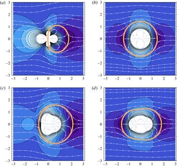
. Inclusion of quadrupole terms results in formation of a closed surface of streamlines separating the flow into the internal and external regions: see (b–d). The external region is singularity-free and can model the flow field of a finite-size swimmer. The separatrix shape can be adjusted by tuning the quadrupole parameters. It can, for example, produce elongated shapes characteristic of the head of a mammalian spermatozoon: see (d). Here colours portray the velocity magnitude, ranging from zero (dark blue) to
 $2V$
(light blue), and white denotes the singularity centre. Arrows indicate the velocity direction in the
 $(z,{\it\rho})$
plane. The thick orange line is the separatrix. (a) Pure dipole:
 ${\it\kappa}=30~{\rm\mu}\text{m}^{3}~\text{s}^{-1}$
,
 $Q_{\Vert }=0~{\rm\mu}\text{m}^{4}~\text{s}^{-1}$
,
 $Q_{\bot }=0~{\rm\mu}\text{m}^{4}~\text{s}^{-1}$
. (b) Source doublet:
 ${\it\kappa}=0$
,
 $Q_{\Vert }=30~{\rm\mu}\text{m}^{4}~\text{s}^{-1}$
,
 $Q_{\bot }=30~{\rm\mu}\text{m}^{4}~\text{s}^{-1}$
. (c) Combined:
 ${\it\kappa}=30~{\rm\mu}\text{m}^{3}~\text{s}^{-1}$
,
 $Q_{\Vert }=30~{\rm\mu}\text{m}^{4}~\text{s}^{-1}$
,
 $Q_{\bot }=30~{\rm\mu}\text{m}^{4}~\text{s}^{-1}$
. (d) Combined:
 ${\it\kappa}=5~{\rm\mu}\text{m}^{3}~\text{s}^{-1}$
,
 $Q_{\Vert }=10~{\rm\mu}\text{m}^{4}~\text{s}^{-1}$
,
 $Q_{\bot }=30~{\rm\mu}\text{m}^{4}~\text{s}^{-1}$
.

2.2. Modelling the swimmer’s near-field
Including quadrupole terms in the expansion of the swimmer velocity field allows us to model the swimmer body and hence avoid the singularities of the multipole expansion at the origin (Stokes Reference Stokes1846). Consider the flow field in the rest frame of the swimmer,
 $\boldsymbol{u}^{rest}=\boldsymbol{u}^{lab}-V\hat{\boldsymbol{e}}_{z}$
, where the laboratory frame flow fields are listed in § 2.1. The flow field of a purely dipolar pusher, given by (2.4) with
 ${\it\kappa}>0$
, is shown in the swimmer rest frame in figure 2(a). Notice a stagnation point a distance
 $z^{\ast }$
directly in front of the swimmer. This point corresponds to
 $u^{D,rest}(z^{\ast })=0$
, which can be inverted to give
 $z^{\ast }=\sqrt{2{\it\kappa}/V}$
. The incoming fluid moves around the stagnation point and the streamlines join again at the singularity. However, the near-field behaviour is unphysical because of the singularity – as expected for a far-field expansion.
Next we consider the source doublet flow given by (2.5) for
 $Q_{sd}\equiv Q_{\Vert }=Q_{\bot }$
and
 $Q_{r}=0$
, and shown in the swimmer rest frame in figure 2(b). For this multipole there is a surface of streamlines connecting two stagnation points in front and behind the swimmer. There is no flow crossing this surface, the separatrix, and hence the singularity region is separated from the rest of the flow. Therefore we can argue that, even though the swimmer is described by point singularities, it has an effective finite size. For a pure source doublet the position of the separatrix can be calculated exactly. Details of this calculations are given in § S3 of the supplementary data. The result is a spherical shell with radius
 $$\begin{eqnarray}a_{sw}=\left(\frac{2Q_{sd}}{V}\right)^{1/3}.\end{eqnarray}$$
Figure 2(c) shows the case when a dipole term is added to the flow field, in addition to the source doublet. If
 $|{\it\kappa}|\ll |Q_{sd}|/a_{sw}$
the separatrix remains approximately spherical with radius
 $a_{sw}$
given by (2.7). If
 $|{\it\kappa}|$
takes larger values, the separatrix changes shape. Indeed, the shape can be adjusted by tuning the dipole and quadrupole parameters. For instance, figure 2(d) shows a separatrix with an elongated shape, approximately
 $4~{\rm\mu}\text{m}$
long and
 $2~{\rm\mu}\text{m}$
wide, characteristic of rod-shaped bacteria or the head of a mammalian spermatozoon (Katz et al.
Reference Katz, Overstreet, Samuels, Niswander, Bloom and Lewis1986). In § S3 of the supplementary data we show that the separatrix exists for all finite values of
 ${\it\kappa}$
provided
 $Q_{\bot }>0$
and
 $-1<Q_{\Vert }/Q_{\bot }<2$
, and we derive an explicit expression for its position.
We shall use this result throughout the paper when numerically integrating tracer displacements, as it provides a useful and physically reasonable way of accounting for the near-field structure of flows created by micro-organisms.
2.3. Expansion of the tracer equation of motion
We aim to generate an expression for the tracer displacement as a power series in
 $1/r$
. The tracer particle is advected directly by the fluid, and its equation of motion is
 $$\begin{eqnarray}\frac{\text{d}\boldsymbol{r}_{T}}{\text{d}t}=\boldsymbol{u}^{sw}(\boldsymbol{r}_{T}-\boldsymbol{R};\hat{\boldsymbol{e}}_{z})+\boldsymbol{u}^{im}(\boldsymbol{r}_{T}-\boldsymbol{R}^{\ast };\hat{\boldsymbol{e}}_{z}),\end{eqnarray}$$
which is an implicit equation subject to the initial condition
 $\boldsymbol{r}_{T}^{int}$
, and where we explicitly write
 $\boldsymbol{u}^{im}$
, the velocity field of the image system, needed when a boundary is present. Equation (2.8) can either be solved numerically or one can proceed analytically if the tracer displacement is small compared to the distance to the swimmer,
 $|{\rm\Delta}\boldsymbol{r}_{T}|\ll |\boldsymbol{r}|~\forall t$
. If the swimming motion is with a constant speed
 $V$
, then taking the time-derivative of this condition yields the equivalent condition
 $\left|\partial _{t}\boldsymbol{r}_{T}(t)\right|=\left|\boldsymbol{u}^{sw}\right|\ll V~\forall t$
.
We change variables in (2.8) to write
 $(\text{d}\boldsymbol{r}_{T}/\text{d}t)=(\text{d}{\rm\Delta}\boldsymbol{r}_{T})/(\text{d}t)=\boldsymbol{u}^{sw}\left(\boldsymbol{r}+{\rm\Delta}\boldsymbol{r}_{T}\right)+\boldsymbol{u}^{im}\left(\boldsymbol{r}^{\ast }+{\rm\Delta}\boldsymbol{r}_{T}\right)$
and expand for small values of
 ${\rm\Delta}\boldsymbol{r}_{T}$
, to give
 $$\begin{eqnarray}\displaystyle \frac{\text{d}{\rm\Delta}\boldsymbol{r}_{T}}{\text{d}t} & = & \displaystyle \left\{\boldsymbol{u}^{sw}[\boldsymbol{r}]+\boldsymbol{u}^{im}[\boldsymbol{r}^{\ast }]\right\}+({\rm\Delta}\boldsymbol{r}_{T}\boldsymbol{\cdot }\boldsymbol{{\rm\nabla}})\left\{\boldsymbol{u}^{sw}[\boldsymbol{r}]+\boldsymbol{u}^{im}[\boldsymbol{r}^{\ast }]\right\}\nonumber\\ \displaystyle & & \displaystyle +\,\frac{1}{2}({\rm\Delta}\boldsymbol{r}_{T}\boldsymbol{\cdot }\boldsymbol{{\rm\nabla}})^{2}\left\{\boldsymbol{u}^{sw}[\boldsymbol{r}]+\boldsymbol{u}^{im}[\boldsymbol{r}^{\ast }]\right\}+O\left(\frac{|{\rm\Delta}\boldsymbol{r}_{T}|}{r}\right)^{3}.\end{eqnarray}$$
To solve for
 ${\rm\Delta}\boldsymbol{r}_{T}$
as a power series in
 $1/r$
we write
 $$\begin{eqnarray}{\rm\Delta}\boldsymbol{r}_{T}(t)={\rm\Delta}\boldsymbol{r}_{T}^{(1)}+{\rm\Delta}\boldsymbol{r}_{T}^{(2)}+{\rm\Delta}\boldsymbol{r}_{T}^{(3)}+\cdots \,,\end{eqnarray}$$
where the terms
 ${\rm\Delta}\boldsymbol{r}_{T}^{(n)}$
scale as
 $r^{-n}$
. Since the swimmer moves with a constant speed
 $V$
along
 $z$
we may write
 $(\text{d}/\text{d}t)=V(\text{d}/\text{d}R_{z})=-V(\text{d}/\text{d}r_{z})=-V(\partial r/\partial z)(\text{d}/\text{d}r)$
. Therefore, the time derivatives
 $\partial _{t}{\rm\Delta}\boldsymbol{r}_{T}^{(n)}$
scale as
 $r^{-n-1}$
. Hence, substituting (2.10) into (2.9), using (2.3) and equating successive powers of
 $1/r$
yields
 $$\begin{eqnarray}\displaystyle & \partial _{t}{\rm\Delta}\boldsymbol{r}_{T}^{(1)}=\boldsymbol{u}^{D}, & \displaystyle\end{eqnarray}$$
 $$\begin{eqnarray}\displaystyle & \partial _{t}{\rm\Delta}\boldsymbol{r}_{T}^{(2)}=\boldsymbol{u}^{Q}, & \displaystyle\end{eqnarray}$$
 $$\begin{eqnarray}\displaystyle & \partial _{t}{\rm\Delta}\boldsymbol{r}_{T}^{(3)}=\boldsymbol{u}^{O}+({\rm\Delta}\boldsymbol{r}_{T}^{(1)}\boldsymbol{\cdot }\boldsymbol{{\rm\nabla}})\boldsymbol{u}^{D}, & \displaystyle\end{eqnarray}$$
 $$\begin{eqnarray}\displaystyle & \partial _{t}{\rm\Delta}\boldsymbol{r}_{T}^{(4)}=\boldsymbol{u}^{H}+({\rm\Delta}\boldsymbol{r}_{T}^{(2)}\boldsymbol{\cdot }\boldsymbol{{\rm\nabla}})\boldsymbol{u}^{D}+({\rm\Delta}\boldsymbol{r}_{T}^{(1)}\boldsymbol{\cdot }\boldsymbol{{\rm\nabla}})\boldsymbol{u}^{Q},\dots , & \displaystyle\end{eqnarray}$$
 $\boldsymbol{u}^{D}=\boldsymbol{u}^{D}(\boldsymbol{r}(t),~\hat{\boldsymbol{e}}_{z})$
and similarly for
 $\boldsymbol{u}^{Q}$
,
 $\boldsymbol{u}^{O}$
etc., into which the image system flow fields are incorporated.
The tracer trajectory can be found by integrating equations (2.11)–(2.14) successively, and substituting the resulting expressions into the higher-order equations of motion. In § S4.1 of the supplementary data we describe this procedure for a swimmer in an unbounded fluid, and in § S4.2 and § S4.3 we repeat the calculations for a swimmer near a no-slip and free-slip boundary respectively.
3. Results: swimmer in an unbounded fluid
We now present results for the trajectory of a tracer particle when a micro-swimmer moves along a straight path of finite length. In § 3.1 we discuss tracer displacements in the radial and swimming direction in the
 $({\it\rho},z)$
plane and in § 3.2 we examine spiralling of tracers in the
 $(x,y)$
plane. In § 3.3 we address the limit of infinite swimming path lengths.
3.1. Tracer loops in the
 $({\it\rho},z)$
plane

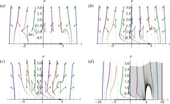
Figure 3 shows the tracer displacements. The values of the swimming speed and the dipole strength were chosen to correspond to an E. coli bacterium (Drescher et al.
Reference Drescher, Dunkel, Cisneros, Ganguly and Goldstein2011). As the run length
 $2L$
between two tumbling events of E. coli varies from 5 to
 $30~{\rm\mu}\text{m}$
(Berg & Brown Reference Berg and Brown1972), we have chosen
 $2L=10~{\rm\mu}\text{m}$
to emphasise the effects of a finite-length swimming path. Different initial tracer positions are depicted by planes of small black dots at
 $z_{T}^{int}=-8,-6,\dots ,6,8~{\rm\mu}\text{m}$
. Coloured dots show the final tracer positions after the swimmer has completed its run. In several cases trajectories are also shown, running from the open circles to the black dots. These results were obtained from a numerical solution of (2.8).
Tracer trajectories and final displacements due to a micro-swimmer in an unbounded fluid. The swimming speed and the dipole strength characteristic for the E. coli bacterium have been used:
 ${\it\kappa}=30~{\rm\mu}\text{m}^{3}~\text{s}^{-1}$
and
 $V=20~{\rm\mu}\text{m}~\text{s}^{-1}$
. Quadrupole strengths
 $Q_{\Vert }=Q_{\bot }=5~{\rm\mu}\text{m}^{4}~\text{s}^{-1}$
were chosen in (b–d) to represent a swimmer with a characteristic size
 $a_{sw}\approx 1~{\rm\mu}\text{m}$
. All higher-order multipole coefficients set to zero. The trajectories are computed using numerical integration of (2.8). Figures (a–c) are in the laboratory frame, where the swimmer moves along a finite line from
 $-5~{\rm\mu}\text{m}$
to
 $L=5~{\rm\mu}\text{m}$
. Initially, tracers are located in planar sheets perpendicular to the
 $z$
-axis at
 $z_{T}^{int}=-8,-6,\dots ,6,8~{\rm\mu}\text{m}$
, uniformly distributed between
 ${\it\rho}=0$
and
 ${\it\rho}=3~{\rm\mu}\text{m}$
, and shown by solid black dots. The final positions of the tracer sheets are depicted by coloured (online) dots. Several trajectories of individual tracers are also shown as thin black lines, running from starting points denoted by open circles to ending points denoted by solid dots. (a) Purely dipolar pusher:
 ${\it\kappa}=30$
,
 $Q_{sd}=0$
. (b) Regularised pusher with finite size:
 ${\it\kappa}=30$
,
 $Q_{sd}=5$
. (c) The equivalent puller with finite size:
 ${\it\kappa}=-30$
,
 $Q_{sd}=5$
. Figure (d) is equivalent to (b) in the rest frame of the micro-swimmer, which itself is located at
 $z=5~{\rm\mu}\text{m}$
; tracers were initially located
 $z_{T}^{int}=2,4,\dots ,16,18~{\rm\mu}\text{m}$
, and final tracer positions are shown after a time
 ${\rm\Delta}t=2L/V$
has passed. Full tracer trajectories are shown for the planar sheet
 $z_{T}^{int}=10~{\rm\mu}\text{m}$
.

Results for a purely dipolar pusher (
 ${\it\kappa}>0$
) are shown in figure 3(a). The tracer trajectories form loops in the region adjacent to the swimming path, where
 $|z_{T}^{int}|\ll L$
, as previously shown by Dunkel et al. (Reference Dunkel, Putz, Zaid and Yeomans2010). The shape of the trajectory is triangular for a dipolar swimmer and is a smaller three-loop structure for a purely quadrupolar swimmer. Notice that the tracer trajectories almost close on themselves, but there is a finite opening of the loop that defines the final tracer displacement
 ${\rm\Delta}\boldsymbol{r}_{T}$
.
Far away from the swimming path, where
 $|\boldsymbol{r}_{T}^{int}|\gg L$
, the final displacement scales as
 $1/r$
and reflects the dipolar flow field because the swimming path approximates a point source,
 $\lim _{r\gg L}{\rm\Delta}\boldsymbol{r}_{T}=\boldsymbol{u}^{sw}{\rm\Delta}t$
, where
 ${\rm\Delta}t=2L/V$
. Additional quadrupole moments do not affect the far-field displacement, as shown in figure 3(b), since these terms decay as
 $1/r^{2}$
. Tracers in front of a pusher are moved forwards, while those behind the swimmer are moved backwards. Displacement along the radial direction is towards the swimming path for
 $|z_{T}^{int}|<L$
and away from the swimming path for
 $|z_{T}^{int}|>L$
. For the equivalent puller (
 ${\it\kappa}\rightarrow -{\it\kappa}$
) the tracers move over the loops in the opposite direction and the displacement in the far-field reverses sign, as shown in figure 3(c).
Closer to the swimming path the tracer displacement does not simply reflect the flow field as the higher-order advective terms in (2.9) become significant. In other words, there is interference between the tracer displacements caused by different multipole components of the swimmer’s velocity field, as seen in the second term of (2.13). We observe that, predominantly, tracer trajectories are larger as the initial distance to the swimming path
 ${\it\rho}_{T}^{int}$
decreases. For tracers that start adjacent to the swimming path, where
 $|\boldsymbol{r}_{T}^{int}|\ll L$
, the final tracer displacement vanishes along the
 ${\it\rho}$
direction. Along the
 $z$
direction it becomes increasingly negative as
 ${\it\rho}$
decreases, for purely dipolar pushers and pullers alike (Pushkin et al.
Reference Pushkin, Shum and Yeomans2013). However, as shown in figure 3(a), it becomes unphysical to use the pure dipolar swimmer model for tracers close to the swimmer where we expect entrainment in the forward direction. Furthermore, the pure dipole model neglects the effects of finite body size important for tracers close to the swimmer, as discussed in § 2.2.
Therefore, we present results in figure 3(b,c) for tracer trajectories near a finite-size swimmer obtained by taking
 $Q_{\Vert }=Q_{\bot }=5~{\rm\mu}\text{m}^{4}~\text{s}^{-1}$
, corresponding to a swimmer with a characteristic size
 $a_{sw}\approx 1~{\rm\mu}\text{m}$
. The effect of the finite swimmer body size is clearly seen in the transition from backward displacement to forward entrainment for tracers with an initial position in the middle of the swimming path, at
 $z_{T}^{int}=0$
, around
 ${\it\rho}_{T}^{int}\approx 0.4~{\rm\mu}\text{m}$
. This transition can be calculated analytically for particles initially located close to the swimming path, i.e. in the limit
 $|\boldsymbol{r}_{T}^{int}|\ll L$
. In § 3.3 we present a detailed calculation and discussion of entrainment effects due to quadrupolar and higher-order terms.
The finite swimmer body size is also responsible for the shape of the tracer trajectories around
 $z_{T}^{int}=5$
. This becomes apparent in figure 3(d), where the trajectories are plotted in the rest frame of the swimmer. Here the tracer trajectories are explicitly shown for
 $z_{T}^{int,rest}=10~{\rm\mu}\text{m}$
and final displacements are shown for
 $z_{T}^{int,rest}=2,4,\dots ,18~{\rm\mu}\text{m}=z_{T}^{int,lab}+10~{\rm\mu}\text{m}$
compared to the laboratory frame. The tracers are advected by the flow, following a trajectory around the swimmer located at
 $z=5~{\rm\mu}\text{m}$
, and ending up in the same positions as the tracers in figure 3(b). The trajectories do not cross the separatrix around the swimmer, as discussed in § 2.2.
3.2. Azimuthal tracer displacements
Swimmers that rotate as they swim, such as numerous biological cells that propel by rotating their flagella, will also displace tracers in the azimuthal direction. Hence, a tracer trajectory will spiral about the direction of the swimmer. Since swimmers are torque-free as well as force-free, their heads and tails rotate in the opposite directions and may cause the tracer spiral trajectories to change chirality as the swimmer passes by. The resulting net azimuthal tracer displacement is far from obvious and will depend on the distance between the tracer and the swimmer path. We describe it using analytical results for tracers far from the swimmer path and numerical results for tracers closer to the swimmer path.
Far from the swimming path an analytic expression showing the contributions of the different multipoles to the tracer displacements follows from equations (S4.3)–(S4.8) of the supplementary data. Let us consider swimmers with a finite path from
 $-L$
to
 $L$
and tracers located initially in the mid-plane
 $z_{T}^{int}=0$
. To the lowest orders in
 ${\it\rho}^{-1}$
, where
 ${\it\rho}\gg L$
and noting that we use the shorthand notation
 ${\it\rho}\equiv {\it\rho}_{T}^{int}$
, the tracer displacement is
 $$\begin{eqnarray}{\rm\Delta}\boldsymbol{r}_{T}^{L}=-\frac{{\it\kappa}}{V}\frac{2{\it\rho}L}{r_{L}^{3}}\hat{\boldsymbol{e}}_{{\it\rho}}+\frac{2L^{3}(Q_{\Vert }-2Q_{\bot })-(Q_{\Vert }+Q_{\bot })L{\it\rho}^{2}}{Vr_{L}^{5}}\hat{\boldsymbol{e}}_{z}+\frac{O_{r}}{V}\frac{6{\it\rho}L}{r_{L}^{5}}\hat{\boldsymbol{e}}_{{\it\phi}}+O\left(\frac{1}{{\it\rho}^{3}}\right),\end{eqnarray}$$
where
 $r_{L}^{2}=L^{2}+{\it\rho}^{2}$
. The first, dipolar, term confirms our conclusion that for a pusher (puller) the tracer is attracted to (repelled from) the swimming path. The second, quadrupolar, term corresponds to displacement along the swimming direction. The third term in (3.1), leading to azimuthal tracer displacement, is the octupolar rotlet. It is notable that the lower-order quadrupolar rotlet term does not appear here because, due to the forward–backward symmetry of the quadrupole rotlet velocity field component, the tracer is rotated in one direction by the head but then in the opposite direction by the tail through an equal angle. This angle, which may be relevant to fluid stirring, is
 $$\begin{eqnarray}{\rm\Delta}{\it\phi}_{T}=\frac{{\rm\Delta}r_{T}^{{\it\phi}}}{{\it\rho}}=-\frac{2Q_{r}}{V}\left(\frac{1}{{\it\rho}^{3}}-\frac{1}{r_{L}^{3}}\right)+O\left(\frac{1}{{\it\rho}^{4}}\right),\end{eqnarray}$$
using equation (S4.8) of the supplementary data. For long swimming path lengths
 ${\rm\Delta}{\it\phi}_{T}$
tends to a finite value for a given value of
 ${\it\rho}$
.
Close to the swimmer path the expression (3.1) is invalid as the higher-order terms become important. Physically, these terms correspond to interference between the tracer displacements. In particular, the tracer displacement due to the dipole and the quadrupole rotlet components interfere in (2.14). Hence, the cancellation of the net azimuthal tracer displacement due to the forward–backward symmetry of the quadrupole rotlet velocity field does not occur even for tracers initially placed in the mid-plane. Therefore we should expect enhanced fluid stirring in the azimuthal direction near the swimmer. In the limit
 $|\boldsymbol{r}_{T}^{int}|\ll L$
this effect can be quantified analytically and we will present these results in § 3.3. Here we analyse the enhancement of azimuthal stirring close to the swimmer for a finite swimming path using numerical calculations.
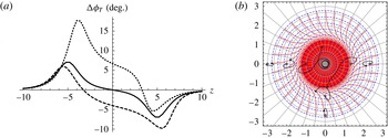
Figure 4 shows the net tracer displacement in the azimuthal direction for a finite-size swimmer having the quadrupole rotlet strength
 $Q_{r}=10~{\rm\mu}\text{m}^{4}~\text{s}^{-1}$
. The enhancement of azimuthal stirring due to interference of the dipole and quadrupole rotlet terms is highlighted in figure 4(a). When
 ${\it\kappa}=0$
, tracers starting at
 $z_{T}^{int}=0$
have the net azimuthal displacement
 ${\rm\Delta}{\it\phi}_{T}=0$
. However, addition of a positive (pusher) dipole term leads to a significant increase of the displacement. A negative (puller) dipole term would also result in a significant displacement, though of a lesser magnitude than for a pusher of the same absolute dipole strength. At the two extrema
 $z_{T}^{int}=\pm L$
tracers are only rotated in one direction by the head (or tail). Inserting the parameters of figure 4(a) and
 $L\rightarrow 2L$
into (3.2) gives
 ${\rm\Delta}{\it\phi}_{T}=\mp 7.1^{\circ }$
at
 $z_{T}=\pm 5~{\rm\mu}\text{m}$
, in good agreement with the numerical results. At larger
 $z$
the interference effect becomes negligible and the
 ${\rm\Delta}{\it\phi}_{T}$
corresponding to different
 ${\it\kappa}$
values converge on the same curve.
Azimuthal tracer displacement due to a rotating micro-swimmer moving along a finite path, from
 $-5$
to
 $5~{\rm\mu}\text{m}$
. Parameters used are
 ${\it\kappa}$
variable,
 $Q_{r}=10~{\rm\mu}\text{m}^{4}~\text{s}^{-1}$
,
 $Q_{\Vert }=Q_{\bot }=1~{\rm\mu}\text{m}^{4}~\text{s}^{-1}$
,
 $V=20~{\rm\mu}\text{m}~\text{s}^{-1}$
, and all other multipole coefficients are set to zero. (a) Dependence of the azimuthal displacement on
 ${\it\kappa}$
. Initially, tracers are located along a line with
 ${\it\rho}=2~{\rm\mu}\text{m}$
and
 $z_{T}^{int}\in [-10,10]~{\rm\mu}\text{m}$
. Final tracer positions are found numerically for
 ${\it\kappa}=0$
(solid),
 ${\it\kappa}=+30$
(dotted), and
 ${\it\kappa}=-30~{\rm\mu}\text{m}^{3}~\text{s}^{-1}$
(dashed). (b) Displacements projected on the
 $(x,y)$
plane, with
 $\hat{\boldsymbol{e}}_{z}$
pointing into the paper;
 ${\it\kappa}=30~{\rm\mu}\text{m}^{3}~\text{s}^{-1}$
. Tracers are initially located in the plane
 $z_{T}^{int}=0$
, distributed on a grid, shown in light grey, with
 ${\it\rho}_{T}^{int}\in [0,3]~{\rm\mu}\text{m}$
with spacing
 $h_{{\it\rho}}=1/3~{\rm\mu}\text{m}$
and
 ${\it\phi}_{T}^{int}\in [-{\rm\pi},{\rm\pi}]$
with spacing
 $h_{{\it\phi}}=2{\rm\pi}/36=10^{\circ }$
. The final tracer displacement is shown by means of the transformed grid. Examples of tracer trajectories, initially located at
 ${\it\rho}_{T}^{int}=1,4/3,\dots ,3~{\rm\mu}\text{m}$
, run from open circles to black dots.

Figure 4(a) shows that overall pushers are more efficient at stirring fluid in the azimuthal direction than pullers of the same absolute dipole strength. This observation has a simple explanation: in (3.1) we have shown for a finite straight swimming path that tracers are attracted to the path if the swimmer is a pusher and repelled from it if the swimmer is a puller. Consequently, tracers spend more time closer to the path of a pusher and the interference effect is stronger. As the attraction/repulsion effect decays with the swimming path length
 $L$
, this difference between pushers and pullers wanes accordingly. Indeed, we will show in § 3.3 that for an infinite swimmer path the azimuthal tracer displacement is dominated by a term proportional to
 ${\it\kappa}Q_{r}/V^{2}$
that has the same magnitude for pushers and pullers of equal absolute dipole strength.
In figure 4(b) the tracer displacement is shown in the
 $(x,y)$
plane for tracers initially located at
 $z_{T}^{int}=0$
for
 ${\it\kappa}>0$
. Far away from the swimming path, whilst being attracted to the swimming path, the tracers are first rotated in the negative (anticlockwise)
 ${\it\phi}$
direction as the swimmer moves from
 $-L$
to 0, then back in the positive
 ${\it\phi}$
direction as the swimmer moves from 0 to
 $L$
. For example, the tracer trajectories starting between
 ${\it\rho}_{T}^{int}=2~{\rm\mu}\text{m}$
and
 $3~{\rm\mu}\text{m}$
show this well. The magnitude of the rotation is again predicted by (3.2). Close to the swimming path there is a strong rotation of tracer particles in the positive (clockwise)
 ${\it\phi}$
direction. This positive angular displacement corresponds to the dotted line in figure 4(a). In particular, the tracer trajectory starting at
 ${\it\rho}_{T}^{int}=1~{\rm\mu}\text{m}$
illustrates that a pusher first attracts the tracer particle towards the swimming path, rotates it several times about the
 $z$
-axis, and then repels it back to a
 ${\it\rho}$
value close to the initial value
 ${\it\rho}_{T}^{int}$
.
3.3. Tracer motion in the limit
$|\boldsymbol{r}_{T}^{int}|\ll L$

We now consider tracer particles which are located near a long swimming path, so that
 $|\boldsymbol{r}_{T}^{int}|\ll L$
. For
 $L\rightarrow \infty$
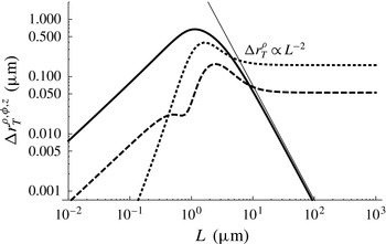
the lowest-order expression for the net tracer displacement (3.1) vanishes. Physically this means that tracer trajectories become, generally, almost closed loops. Indeed, numerical results for the tracer displacement as a function of the swimming path length
 $L$
, presented in figure 5, show that the
 ${\it\rho}$
component of the displacement decays as
 ${\rm\Delta}\boldsymbol{r}_{T}^{{\it\rho}}\sim L^{-2}$
. This dependence follows directly from the first term in (3.1). The
 $z$
and
 ${\it\phi}$
components, however, remain finite for large swimming path lengths. In order to describe this behaviour analytically we need to take into account higher-order terms in the expansion for the tracer displacement (2.10).
Dependence of the tracer displacement
 ${\rm\Delta}\boldsymbol{r}_{T}$
on the swimming path length
 $2L$
. Initially, the tracer is located at
 $z_{T}^{int}={\it\phi}_{T}^{int}=0$
and
 ${\it\rho}_{T}^{int}=2~{\rm\mu}\text{m}$
. Final displacements, obtained numerically, in the
 ${\it\rho},{\it\phi},z$
directions are denoted by the solid, dotted and dashed lines respectively. Parameters used are
 $V=20~{\rm\mu}\text{m}~\text{s}^{-1}$
,
 ${\it\kappa}=30~{\rm\mu}\text{m}^{3}~\text{s}^{-1}$
,
 $Q_{\Vert }=Q_{\bot }=5~{\rm\mu}\text{m}^{4}~\text{s}^{-1}$
and
 $Q_{r}=1~{\rm\mu}\text{m}^{4}~\text{s}^{-1}$
. All other multipole coefficients are set to zero.

In § S4.1 of the supplementary data we compute contributions up to the sixth order inclusive, which gives us enough information to study both a short swimming path (3.1) and also the two leading-order contributions in powers of
 $1/{\it\rho}$
along each of the directions
 $z$
,
 ${\it\rho}$
and
 ${\it\phi}$
in the limit
 $L\rightarrow \infty$
. Hence, writing terms up to
 $O(1/{\it\rho}^{6})$
, we obtain the final tracer displacement
 $$\begin{eqnarray}\displaystyle {\rm\Delta}\boldsymbol{r}_{T}^{\infty } & = & \displaystyle \left(-\frac{{\rm\pi}{\it\kappa}^{2}}{16V^{2}}\frac{1}{{\it\rho}^{3}}+\frac{9{\rm\pi}(9Q_{\Vert }^{2}+14Q_{\Vert }Q_{\bot }+41Q_{\bot }^{2})}{1024V^{2}}\frac{1}{{\it\rho}^{5}}-\frac{9{\rm\pi}{\it\kappa}(3O_{\Vert }+7O_{\bot })}{256V^{2}}\frac{1}{{\it\rho}^{5}}\right)\hat{\boldsymbol{e}}_{z}\nonumber\\ \displaystyle & & \displaystyle +\,\left(\frac{9{\rm\pi}{\it\kappa}Q_{r}}{8V^{2}}\frac{1}{{\it\rho}^{4}}-\frac{225{\rm\pi}(2Q_{r}(O_{\bot }+O_{\Vert })+O_{r}(Q_{\bot }+3Q_{\Vert })+2{\it\kappa}H_{r})}{512V^{2}}\frac{1}{{\it\rho}^{6}}\right)\hat{\boldsymbol{e}}_{{\it\phi}}.\nonumber\\ \displaystyle & & \displaystyle\end{eqnarray}$$
First, consider the final tracer displacement in the swimming direction,
 $\hat{\boldsymbol{e}}_{z}$
. Far from the swimmer, for large
 ${\it\rho}$
values, the
 ${\it\kappa}^{2}$
dipole term dictates a tracer displacement along the negative
 $z$
direction that scales as
 ${\rm\Delta}r_{z}\propto {\it\rho}^{-3}$
. This far-field result is the same for both pushers and pullers, since it is proportional to
 ${\it\kappa}^{2}$
. Closer to the swimming path, the negative displacement is countered by a forward entrainment due to the quadrupole term, which is positive for all values of
 $Q_{\Vert }$
and
 $Q_{\bot }$
. We have already seen this behaviour for tracers that start close to the middle of a finite swimming path in figure 3(b). In principle the octupole and higher-order terms, which will depend on individual swimmer details, could contribute to a backward displacement, although eventually a forward entrainment is expected very close to the swimmer due to the no-slip boundary condition at its surface. So, in general, although the expression (3.3) is only guaranteed to be exact in the limit of large
 ${\it\rho}$
, it gives a qualitatively correct picture of tracer displacements even for tracers initially located close to the swimmer. In particular, there is a characteristic critical radius
 ${\it\rho}={\it\rho}_{c}$
where the displacement in the swimmer direction changes sign:
 $$\begin{eqnarray}{\it\rho}_{c}=\frac{3\sqrt{9Q_{\Vert }^{2}+14Q_{\Vert }Q_{\bot }+41Q_{\bot }^{2}-4{\it\kappa}(3O_{\Vert }+7O_{\bot })}}{8{\it\kappa}}.\end{eqnarray}$$
For
 ${\it\rho}\gg {\it\rho}_{c}$
the far-field dipole approximation holds, whereas for
 ${\it\rho}\ll {\it\rho}_{c}$
the near-field dominates the tracer displacement. Notice that substituting the parameters of figure 3(b) into (3.4) gives
 ${\it\rho}_{c}=0.5~{\rm\mu}\text{m}$
, in reasonable agreement with the numerical results, given the small value
 $L=5$
chosen to emphasise the effects of a finite swimming path.
In the angular direction,
 $\hat{\boldsymbol{e}}_{{\it\phi}}$
, (3.3) shows that the displacement of tracer particles about the
 $z$
-axis scales as
 ${\rm\Delta}r^{{\it\phi}}\propto {\it\kappa}Q_{r}{\it\rho}^{-4}$
far from the swimming path. Therefore a micro-swimmer with a head (tail) rotating in the (anti-) clockwise direction will stir particles in the anticlockwise direction in the far-field. Dividing by the trajectory circumference
 $2{\rm\pi}{\it\rho}$
, the number of revolutions made by a tracer scales as
 ${\it\rho}^{-5}$
. Inserting the parameters of figure 4(b) into (3.3) gives
 ${\sim}2.7$
revolutions for a tracer particle with
 ${\it\rho}_{T}^{int}=1~{\rm\mu}\text{m}$
, which is in reasonable quantitative agreement with the figure where the particle is rotated
 ${\sim}3.2$
times around the swimming path.
Along the radial direction,
 $\hat{\boldsymbol{e}}_{{\it\rho}}$
, our calculations show that all contributions to the final tracer displacement vanish up to order
 $O({\it\rho}^{-7})$
and numerical integration of the implicit differential equation (2.8) also shows no resultant displacement to within machine precision. Although for
 $L=\infty$
the tracer does move along
 $\hat{\boldsymbol{e}}_{{\it\rho}}$
, it returns to its original distance from the swimming path
 ${\it\rho}_{int}$
once the swimmer has moved past. Physically, this is reasonable as we are assuming the fluid to be incompressible. That is, if
 ${\rm\Delta}r_{T}^{{\it\rho}}$
had a finite negative (positive) value, constant for all initial tracer positions
 $z_{T}^{int}$
along the infinite swimming path, then this would lead to a singular accumulation (depletion) of particles at the
 $z$
-axis, which would violate incompressibility. The final tracer displacement must be divergence-free and hence the radial displacement vanishes for a long swimming path.
4. Results: swimmer moving parallel to a boundary
In experiments, micro-swimmers are often observed in the presence of boundaries and in biological systems micro-organisms often tend to accumulate near surfaces, as described by Berke et al. (Reference Berke, Turner, Berg and Lauga2008), Li et al. (Reference Li, Bensson, Nisimova, Munger, Mahautmr, Tang, Maxey and Brun2011) and Spagnolie & Lauga (Reference Spagnolie and Lauga2012). Therefore, we next present results for tracer trajectories and final displacements due to a micro-swimmer moving parallel to a planar surface. Compared to a swimmer moving in an unbounded fluid with swimming path length
 $L$
, the swimmer body size
 $a_{sw}$
(equations (S3.5) and (S3.9) of the supplementary data) and the entrainment radius
 ${\it\rho}_{c}$
(3.4), there is an additional length scale in this system, the distance
 $H$
between the swimmer and the boundary.
As in § 3, we start by describing numerical results for the tracer trajectories, where parameters were chosen to represent a typical E. coli bacterium near a no-slip boundary in figure 6. We also show analogous results for a free-slip boundary in figure 7 and summarise similarities and differences between the two boundary types. In analogy to § 3, in the supplementary data we aim to develop a more quantitative understanding of tracer motion, particularly in terms of the distance
 $H$
. In § S4.2 and § S4.3 of the supplementary data we compute tracer displacements up to fourth order, for the no-slip and free-slip boundaries respectively, and in § S6 and § S7 we discuss these in the limit of an infinite swimming path.
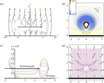
Numerical results for tracer displacements and trajectories due to a micro-swimmer moving along a finite path parallel to a no-slip boundary. The units of length and time are
 ${\rm\mu}\text{m}$
and s. The swimming path is from
 $-5$
to 5. The boundary is denoted by a thick black line. Several tracer trajectories are shown as thin black curves, running from starting points denoted by open circles to ending points denoted by solid red dots. The trajectories were computed using numerical integration of (2.8). Parameters used are
 ${\it\kappa}=30$
,
 $Q_{\Vert }=Q_{\bot }=1$
,
 $V=20$
. All other multipoles are set to zero. (a) Tracer displacements in the
 $x{-}z$
plane for
 $H=1.5$
. Initially, tracers are located in sheets perpendicular to the boundary at
 $y_{T}^{int}=0$
and
 $z_{T}^{int}=-8,-6,\dots ,6,8$
, uniformly distributed between
 $x_{T}^{int}=0$
and 4.5, as shown by black dots. The final positions are shown by dots in various colours (online). (b) An
 $x{-}y$
cross-section showing the displacement along the
 $z$
-axis of tracers which start in the plane
 $z_{T}^{int}=0$
for
 $H=1.5$
. Colours indicate the magnitude of the displacement. White indicates strong forward entrainment (displacements
 ${>}1.5$
). (c) Dependence of tracer trajectories in the
 $x{-}z$
plane on distance from the boundary
 $H$
. The
 $x$
-axis is scaled with respect to
 $H$
but the
 $z$
-axis is not scaled. Initially, tracers are located along the line
 $y_{T}^{int}=z_{T}^{int}=0$
. The final positions are shown by continuous lines in red, orange, green, blue and purple for
 $H=1,1.2,1.4,2,4$
respectively. (d) An
 $x{-}y$
cross-section showing the in-plane displacement of tracers which start in the plane
 $z_{T}^{int}=0$
. The swimmer rotation strength
 $Q_{r}=0$
. Tracers are initially uniformly distributed on a grid with
 $0\leqslant x_{T}^{int}\leqslant 4$
and
 $-2\leqslant y_{T}^{int}\leqslant 2$
with spacing
 $h=1/5$
. The final displacement is depicted by means of the transformed grid.

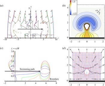
Numerical results for tracer displacements and trajectories due to a micro-swimmer moving along a finite path parallel to a free-slip boundary. Apart from the boundary type, this figure is identical to figure 6.

In figures 6 and 7 we show tracer displacements and several trajectories for a swimmer moving from
 $-L$
to
 $+L$
parallel to the boundary. These results were obtained by numerically integrating equation (2.8) including the appropriate image term. The image system of a swimmer near a free-slip boundary is simply a mirror swimmer. Near a no-slip boundary, however, the image of a dipolar pusher (puller) is the equivalent puller (pusher) plus more complex terms of quadrupolar and octupolar structure (see § S2.6 of the supplementary data). To see the effect of the boundary it is useful to compare with figures 3 and 4 for swimming in an infinite fluid,
 $H=\infty$
. Close to the swimming path the tracer displacements are almost independent of
 $H$
and the results of § 3.3 hold. However, far from the swimmer, and also between the swimmer and the surface, there are boundary effects because here the distances to the swimmer and to the image are comparable.
Figures 6(a) and 7(a) show the tracer displacement in the
 $(x,z)$
plane. Far away from the swimmer and the free-slip boundary the trajectories are doubled in size, since the swimmer and its mirror image cooperate. For the no-slip boundary, however, the dipolar terms of the swimmer and image cancel (in equation (S4.21) of the supplementary data), so that the tracer trajectories are no longer triangular loops as for a dipolar swimmer but instead the dominant quadrupolar terms give a smaller three-loop trajectory.
Consider now what happens close to the boundary. Our first observation is that despite a no-slip boundary condition, there is a significant forward displacement of tracer particles between the swimming path and the boundary. Also, for a finite swimming path, tracers that start at
 $z>0$
tend to be displaced forwards. For the free-slip boundary this effect is about three times larger with the absence of the no-slip constraint.
This is emphasised in figures 6(b) and 7(b), which show the longitudinal displacement in the
 $x{-}y$
plane for tracers initially at
 $z=0$
. The maximum forward displacement between swimmer and boundary is about
 $0.3~{\rm\mu}\text{m}$
in the no-slip case compared to
 $1~{\rm\mu}\text{m}$
for the free-slip boundary. Comparison of figures 6(b) and 7(b) shows that the longitudinal displacement is positive in the far-field for the no-slip boundary but negative for the free-slip boundary.
Figures 6(c) and 7(c) show the dependence of the tracer displacements on
 $H$
. Note that in this figure the
 $x$
-axis is scaled with respect to
 $H$
but the
 $z$
-axis is not scaled. The purple curve for
 $H=4~{\rm\mu}\text{m}$
approaches the unbounded swimmer case. As
 $H$
decreases, the forward displacement between the swimmer and the boundary increases as
 ${\it\kappa}^{2}/V^{2}H^{3}$
, and is maximum at
 ${\it\zeta}=0$
and
 ${\it\zeta}_{m}=0.3$
for the free-slip and no-slip boundary respectively. For small
 $H$
values, compared to the other system length scales, the near-field entrainment interferes with the forward displacement at the boundary. For the no-slip boundary this shifts the maximum to lower
 ${\it\zeta}$
values and for the free-slip boundary this merges the entrainment of the boundary and near-field, so that at
 $H=a_{sw}$
the swimmer acts like a little bulldozer.
In figures 6(d) and 7(d) the tracer displacements in the transverse directions, along
 $x$
and
 $y$
, are shown in the
 $(x,y)$
plane for
 $z=0$
. Despite the fact that
 $Q_{r}=0$
, representing a non-rotating swimmer, we find significant mixing of tracer particles in the transverse directions, up to
 $0.8~{\rm\mu}\text{m}$
close to the swimming path for a no-slip boundary. With decreasing
 $H$
, the strength of this effect increases as
 ${\it\kappa}Q_{\bot }/V^{2}H^{4}$
, independently of
 $Q_{\Vert }$
. Furthermore, tracers near a free-slip boundary are not attracted towards the swimming path, as is the case in the limit
 $H\rightarrow \infty$
given by (3.1), but towards the boundary instead.
In § S6 and § S7 of the supplementary data we describe the tracer motion near a free-slip and no-slip surface respectively in terms of a perturbative expansion analogous to that in § 3.3. Hence, we find analytic expressions in terms of the experimental parameters
 $H,V,L,{\it\kappa}$
, etc., for the additional boundary-induced entrainment and transverse stirring of tracer particles.
5. Discussion
We have studied the way in which an axisymmetric swimmer moves tracer particles as it swims through a fluid, concentrating on straight swimming trajectories of finite and infinite length, in an unbounded fluid and parallel to a surface, considering both slip and no-slip boundary conditions. Numerical results were obtained by integrating the equations of tracer motion. Analytical results followed from expanding the tracer displacement in powers of
 $r^{-1}$
, the inverse distance between swimmer and tracer.
We started by considering a finite swimming path from
 $z=-L$
to
 $L$
. Far from the swimmer the tracer particles move in loop-like trajectories with a size that scales as
 ${\it\kappa}/{\it\rho}$
, where
 ${\it\kappa}$
is the strength of the swimmer dipole moment and
 ${\it\rho}=\min r(t)$
, the distance between tracer and swimming path. As the swimmer trajectory becomes infinitely long the tracer trajectories tend to almost closed loops, but a finite final net displacement remains that is backwards relative to the swimming direction and scales as
 $-{\it\kappa}^{2}/{\it\rho}^{3}$
. The introduction of a slip surface doubles the loops in size, and for an infinite swimming path enhances the final tracer displacement by a factor four. For a no-slip boundary, however, the far-field tracer loops are much smaller, with a final radial displacement that scales as
 ${\it\kappa}/{\it\rho}^{3}$
for a finite swimmer trajectory crossing over to a scaling
 $+{\it\kappa}^{2}/{\it\rho}^{5}$
in the swimming direction for an infinite swimming path.
Closer to the swimmer the tracer particles still move in loop-like trajectories. However, they are now entrained by the swimmer, showing a significant net forward displacement. We show that this can usefully be modelled by including quadrupolar terms in the flow field. These lead to a surface around the singularity across which there is no flow, mimicking a finite swimmer size and removing the problem of the singularities in the multipole expansion of the flow field. A proper combination of the quadrupole coefficients can model the near-field of swimmers of the elongated shapes typical of many micro-organisms.
Along the surface itself tracer particles are displaced forwards along the swimming direction, both for slip and for no-slip boundaries, for pushers and for pullers. As the distance
 $H$
between the boundary and the swimming path increases, the forward displacement wanes as
 ${\it\kappa}^{2}/H^{3}$
.
To quantify these effects consider a typical swimmer with parameters chosen to represent an E. coli bacterium,
 ${\it\kappa}=30~{\rm\mu}\text{m}^{3}~\text{s}^{-1},V=20~{\rm\mu}\text{m}~\text{s}^{-1}$
and
 $L=5~{\rm\mu}\text{m}$
. A tracer particle initially located at
 $z_{T}^{int}=0$
and
 ${\it\rho}_{T}^{int}=1.5~{\rm\mu}\text{m}$
follows a triangular loop-like trajectory of size
 ${\sim}1~{\rm\mu}\text{m}$
. Its final displacement is
 ${\sim}0.25~{\rm\mu}\text{m}$
against the swimming direction. The crossover from final backward displacement to forward entrainment, if we take the quadrupole strengths
 $Q_{\Vert ,\bot }=5~{\rm\mu}\text{m}^{4}~\text{s}^{-1}$
, occurs at a distance
 ${\it\rho}_{c}\sim 3Q_{\Vert ,\bot }/{\it\kappa}\sim 0.5~{\rm\mu}\text{m}$
from the swimming path. Close to a slip boundary, if the swimmer moves at a distance
 $H=1.5~{\rm\mu}\text{m}$
, the tracer particle is displaced
 ${\sim}0.9~{\rm\mu}\text{m}$
along the swimming direction, compared to
 ${\sim}0.3~{\rm\mu}\text{m}$
for a no-slip boundary.
Non-rotating swimmers do not displace tracers in the azimuthal direction when they swim far from the boundaries. A rotating swimmer with the head rotating in the clockwise direction (and the tail rotating in the anticlockwise direction) rotates tracer particles in the anticlockwise direction. For example, for a swimmer with rotation strength
 $Q_{r}=10~{\rm\mu}\text{m}^{4}~\text{s}^{-1}$
, a tracer particle initially located a distance
 ${\it\rho}=1~{\rm\mu}\text{m}$
from the swimming path can be rotated up to
 ${\sim}3$
times around it. For a pusher this stirring effect is larger than for a puller, as it first attracts a tracer towards the swimming path, where the azimuthal flow is stronger, before repelling it back to its initial radius
 ${\it\rho}_{T}^{int}$
.
Close to a boundary even non-rotating swimmers create fluid flows in the plane perpendicular to the swimming direction. This may be ecologically significant as a mechanism for resuspension of small sedimented particles. The strength of this effect scales as the product
 ${\it\kappa}Q_{\bot }$
.
Loop-like tracer trajectories have been observed in several experiments with biological (Kurtuldu et al. Reference Kurtuldu, Guasto, Johnson and Gollub2011) and non-biological swimmers (Thutupalli Reference Thutupalli2014), but quantitative matching of our results to experiment at this point is difficult due to the unpredictability of swimmer trajectories and insufficient quality of experimental data. Currently, however, new experimental techniques are being developed that could allow simultaneous observation of multiple trajectories of tracer particles (Molaei et al. Reference Molaei, Barry, Stocker and Sheng2014). Also, development of artificial micro-swimmers that are more easily controllable could provide the data for a quantitative match between theory and experiment.
Throughout the paper we neglect the smearing effect of Brownian fluctuations on the tracer trajectories. Its relative importance depends on the physical size of advected particles and is typically weak for particles larger than one micron (Leptos et al. Reference Leptos, Guasto, Gollub, Pesci and Goldstein2009). Moreover, the effect of Brownian fluctuations on mixing can be accounted for by adding the Brownian and the biogenic contributions to the effective tracer diffusion coefficient (Pushkin & Yeomans Reference Pushkin and Yeomans2014).
Our results connect well to recent works (Pushkin & Yeomans Reference Pushkin and Yeomans2013; Morozov & Marenduzzo Reference Morozov and Marenduzzo2014; Thiffeault Reference Thiffeault2014) that address recent observations of non-Gaussian tracer displacement (Leptos et al.
Reference Leptos, Guasto, Gollub, Pesci and Goldstein2009; Kurtuldu et al.
Reference Kurtuldu, Guasto, Johnson and Gollub2011; Jepson et al.
Reference Jepson, Martinez, Schwarz-Linek, Morozov and Poon2013; Miño et al.
Reference Miño, Dunstan, Rousselet, Clément and Soto2013). Our expressions could input into a more accurate calculation of the displacements distribution and of the diffusion coefficient by accounting for a finite swimmer size. This latter provides a cut-off for large particle displacements. Hence, in the long run the distribution will converge to a Gaussian. Furthermore, we expect enhanced biomixing in fluid layers near boundaries since tracers are entrained farther. This prediction is in agreement with the experiments by Mino et al. (Reference Mino, Mallouk, Darnige, Hoyos, Dauchet, Dunstan, Soto, Wang, Rousselet and Clement2011), but it provides an alternative explanation for this effect. Our expressions could allow for a first approximation of the effective, anisotropic, tracer diffusion coefficients near an interface as a function of
 $H$
.
This paper has only considered swimming paths oriented parallel to the boundary, motivated by experiments by Molaei et al. (Reference Molaei, Barry, Stocker and Sheng2014) that show that the tumbling of wild-type E. coli is suppressed up to distances
 $20~{\rm\mu}\text{m}$
from a no-slip surface, and when they tumble the reorientations are largely skewed towards the surface-parallel directions. Nevertheless, the analysis may easily be extended for swimmers approaching or leaving the boundary at a given angle or along a defined trajectory (Spagnolie & Lauga Reference Spagnolie and Lauga2012; Zöttl & Stark Reference Zöttl and Stark2012) or moving in, say, a circular trajectory (Lauga et al.
Reference Lauga, DiLuzio, Whitesides and Stone2006; Di Leonardo et al.
Reference Di Leonardo, Dell’Arciprete, Angelani and Iebba2011). Moreover, it would be of interest to understand the effect of other types of confinement, such as between two parallel flat plates or inside a thin liquid film on tracer trajectories. The single swimmer problem provides a step towards estimating the tracer motion and the increase in tracer diffusion due to a suspension or beam of swimmers, and how this is altered by the presence of a boundary.
Acknowledgement
We acknowledge funding from the ERC Advanced Grant MiCE.
Supplementary data
Supplementary data are available at http://dx.doi.org/10.1017/jfm.2015.269.