
1 Introduction
All algebraic varieties considered in the paper are over
 $\mathbb {C}$
. A sextic (surface) is a degree six
 $K3$
-surface in
 $\mathbb {P}^{4}$
; it is the intersection of a cubic and a quadric.
1.1 The principal result
Counting rational curves in projective surfaces is a long standing classical problem in algebraic geometry. Each smooth cubic surface
 $X\subset \mathbb {P}^{3}$
contains exactly
 $27$
lines [Reference Cayley3], whereas a typical quartic surface has no lines at all, and the question changes to bounding the number of lines that a special surface may have. In 1882, Schur [Reference Schur26] constructed a quartic with
 $64$
lines, but the problem was not settled until 1943, when Segre [Reference Segre28] proved that
 $64$
is indeed the maximum. A minor gap in Segre’s proof was discovered and bridged by Rams and Schütt [Reference Rams and Schütt22], and a partial classification of large configurations of lines was given by Degtyarev et al. [Reference Degtyarev, Itenberg and Sertöz9].
Little is known about surfaces
 $X\subset \mathbb {P}^{3}$
of higher degree: in spite of considerable efforts (see recent papers [Reference Elkies10] or [Reference Rams and Schütt23] and references therein), the known bounds are still too far from the known examples. On the other hand, smooth quartics being
 $K3$
-surfaces, one can change the paradigm and consider other polarizations, that is, smooth
 $K3$
-surfaces
 $X\subset \mathbb {P}^{d+1}$
of degree
 $2d$
. In this direction, we do obtain sharp upper bounds and a plethora of examples (see [Reference Degtyarev5], [Reference Degtyarev7]).
Even less is known about rational curves of other degree, even in
 $K3$
-surfaces
 $X\subset \mathbb {P}^{d+1}$
. For conics in quartic surfaces, the best examples have
 $352$
or
 $432$
conics (see [Reference Barth and Bauer1], [Reference Bauer2]), whereas the best known upper bound is
 $5016$
(see [Reference Bauer2] with a reference to Strømme). There also are some asymptotic bounds as
 $d\to \infty $
(see [Reference Miyaoka17], [Reference Rams and Schütt24]). In this paper, we suggest to attack the conic problem using a modification of an approach that already proved useful in two similar counting problems (cf. [Reference Degtyarev7], [Reference Degtyarev, Itenberg and Ottem8]). We expect it to work for the “interesting” degrees
 $2\leqslant 2d\leqslant 8$
, where the surfaces are complete intersections, and we test it in the case
 $2d=6$
, sextic surfaces in
 $\mathbb {P}^{4}$
, mainly because we can partially reuse some results of [Reference Degtyarev, Itenberg and Ottem8] in the computation. It is worth emphasizing that, in our approach, we intentionally cut off the lines and work with an abstract combinatorial configuration (dual adjacency graph) of conics, counting both irreducible and reducible ones. Lines are recovered at the very end, when the lattice is embedded to
 $H_2(X)$
, and it is at this point that reducible conics can be told apart. The combinatorial configuration does not always know which of the conics are reducible, see the remark after Theorem 1.1 and Examples 8.4 and 8.6.
The principal result of the paper is proved in §8.1: it is the following sharp upper bound on the number of conics in a smooth sextic surface
 $X\subset \mathbb {P}^{4}$
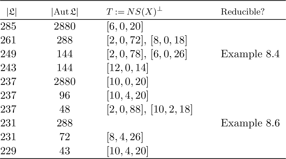
, including a partial classification of large combinatorial configurations of conics. Surprisingly, the extremal surfaces contain no lines, so that all their conics are irreducible.
Theorem 1.1. Up to projective transformation, there are but three smooth sextic
 $K3$
-surfaces
 $X\subset \mathbb {P}^{4}$
with more than
 $260$
conics (irreducible or reducible):
-
1. one real surface
 $X_{285}$
with
$285$
conics, all irreducible, see (8.1), and
-
2. two real surfaces
$X_{261}$
,
$Y_{261}$
, which share the same combinatorial configuration of
$261$
conics, all irreducible, see (8.2) and (8.3), respectively.


The surface
 $Y_{261}$
admits a real form in which all conics are real (moreover, have real points), thus maximizing the number of real conics in a real sextic surface.
In view of [Reference Schütt27], [Reference Shimada29], it seems plausible that the polarized surfaces
 $X_{261}$
and
 $Y_{261}$
should be Galois conjugate; that would explain the fact that they share the same configuration.
Conjecturally, the next value taken by the number of conics in a smooth sextic surface
 $X\subset \mathbb {P}^{4}$
is
 $249$
(see Example 8.4). The known combinatorial configuration of
 $249$
conics is realized by four distinct surfaces; in two of these surfaces, all conics are irreducible, whereas in the two others, there are
 $60$
irreducible conics and
 $189$
reducible ones, composed of the
 $42$
lines contained in the surface. In fact,
 $189$
is the maximal possible number of reducible conics, see Remark 8.5.
1.2 Contents of the paper
In §2, we introduce the arithmetical reduction of the problem, consisting in modifying the Néron–Severi lattice of the surface and replanting the result to an appropriate Niemeier lattice. With future applications in mind, we treat arbitrary smooth
 $2d$
-polarized
 $K3$
-surfaces
 $X\to \mathbb {P}^{d+1}$
. In §3, we describe the principal technical tools used in the computation. We switch to degree
 $2d=6$
, even though most tools should apply to other degrees as well. §§4–7 deal with the computation per se, which was done using GAP [11]; we outline just enough details for the interested reader to be able to reproduce the result. Finally, in §8, we combine our findings to present a formal proof of Theorem 1.1. We also discuss a few interesting examples of large configurations of conics which were discovered in our study of individual Niemeier lattices.
2 The reduction
Throughout the paper, we fix the notation
 $\mathbf {L}$
for a fixed even unimodular lattice of signature
 $(3,19)$
; in other words,
 $\mathbf {L}\cong -2\mathbf {E}_8\oplus 3\mathbf {U}$
is the
 $2$
-homology of a
 $K3$
-surface. All lattices considered are even, and a root is a vector of square
 $\pm 2$
.
2.1 Conics as homology classes
Let
 $\varphi \colon X\hookrightarrow \mathbb {P}^{d+1}$
be a smooth
 $2d$
-polarized
 $K3$
-surface. (If
 $d=1$
, the “smoothness” refers to the ramification locus of
 $\varphi $
, which is two-to-one; otherwise, we assume
 $\varphi $
injective.) The map
 $\varphi $
gives rise to the triple
 $$ \begin{align*} \mathbf{L}\cong H_2(X)\supset NS(X)\ni h_X:=\varphi^*\mathcal{O}_{\mathbb{P}^{d+1}}(1),\quad h_X^2=2d, \end{align*} $$
called the homological type of
 $X\hookrightarrow \mathbb {P}^{d+1}$
. The period
 $\omega _X\in H_2(X;\mathbb {C})$
(the class of a holomorphic two-form on X) defines an orientation on
 $\mathbb {R} h\oplus \mathbb {R}(\mathrm {Re}\,\omega _X)\oplus \mathbb {R}(\mathrm {Im}\,\omega _X)$
and, hence, on any other positive definite three-space in
 $H_2(X;\mathbb {R})$
; this coherent choice of orientations is called the canonical orientation of the homological type. Letting
 $$ \begin{align*} (\mathbf {L}\supset NS\ni h):=(H_2(X)\supset NS(X)\ni h_X), \end{align*} $$
the homological type has the following properties:
-
1. the lattice
$NS$
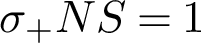
is hyperbolic, that is,
$\sigma _+ NS=1$
; -
2. the sublattice
$NS\subset \mathbf {L}$
is primitive, that is,
$\mathrm {Tors}(\mathbf {L}/\!NS)=0$
; -
3. there is no vector
$e\in NS$
such that
$e^2=-2$
and
$e\cdot h=0$
; -
4. there is no vector
$e\in NS$
such that
$e^2=0$
and
$e\cdot h=2$
; and -
5. if
$d=4$
, then
$h\notin 2 NS$
.



Here, (4) implies that there is no
 $e\in NS$
such that
 $e^2=0$
and
 $e\cdot h=1$
and, hence, the linear system
 $|h|$
is fixed point free, see [Reference Nikulin20], [Reference Saint-Donat25]. Then, by [Reference Saint-Donat25], conditions (4) and (5) are equivalent to the statement that the map
 $X\to \mathbb {P}^{d+1}$
given by
 $|h|$
is birational onto its image. (Strictly speaking, [Reference Saint-Donat25] uses a genus
 $1$
curve rather than class
 $e\in NS$
; however, assuming (3), one of
 $\pm e$
is necessarily nef.)
Due to the global Torelli theorem for
 $K3$
-surfaces [Reference Pjateckiĭ-Šapiro and Šafarevič21], surjectivity of the period map [Reference Kulikov14], and Saint-Donat’s results on projective models of
 $K3$
-surfaces [Reference Saint-Donat25], the converse also holds. The following statement is well known, and various versions thereof appear in virtually any paper on the subject (cf. [Reference Degtyarev, Itenberg and Sertöz9, Th. 3.11] or [Reference Degtyarev6, Th. 7.3]).
Theorem 2.1. An oriented abstract triple
 $\mathbf {L}\supset NS\ni h$
,
 $h^2=2d$
, is isomorphic to the oriented homological type of a smooth
 $2d$
-polarized
 $K3$
-surface X if and only if
 $\mathbf {L}\supset NS\ni h$
has properties (1)–(5). Then, X is a generic member of a connected
 $(20-\mathrm {rk}\,NS)$
-parameter, modulo the group
 $PGL(d+2,\mathbb {C})$
, family of
 $2d$
-polarized
 $K3$
-surfaces.
Given a line
 $L\subset X$
or a conic
 $C\subset X$
(not necessarily irreducible), the homology classes
 $l:=[L]\in NS(X)$
and
 $c:=[C]\in NS(X)$
have the property that
 $$ \begin{align} l^2=c^2=-2,\qquad l\cdot h=1,\quad c\cdot h=2. \end{align} $$
In particular, since the self-intersection is negative, a line or a conic is unique in its class and can be identified with the latter. By the Riemann–Roch theorem, conversely, any class l or
 $c\in NS(X)$
satisfying (2.2) is represented by a unique line or conic, respectively. It follows from the description of the nef cone of X (see, e.g., [Reference Huybrechts13, Cor. 8.2.11]) that irreducible conics are characterized by the property
 $$ \begin{align} \text{a conic }c\in NS(X)\text{ is irreducible iff }c\cdot l\geqslant0\text{ for each line } l\in NS(X). \end{align} $$
2.2 The lattice
$S( NS,h)$

A
 $2d$
-polarized lattice is a lattice
 $NS$
equipped with a distinguished vector
 $h\in NS$
of square
 $2d>0$
. We say that
 $NS\ni h$
is of type I if
 $h\in 2 NS^\vee $
; otherwise,
 $NS\ni h$
is said to be of type II. The graph of lines (
 $n=1$
), conics (
 $n=2$
), and so on of a hyperbolic polarized lattice
 $ NS\ni h$
is the graph
 $$ \begin{align*} \mathrm{Fn}_n(NS,h):=\bigl\{c\in NS\bigm| c^2=-2 \text{ and } c\cdot h=n\bigr\}, \end{align*} $$
where two vertices
 $c_1$
and
 $c_2$
are connected by an edge of multiplicity
 $c_1\cdot c_2$
. Since
 $NS$
is assumed hyperbolic, each set
 $\mathrm {Fn}_n$
is finite; the vertices of
 $\mathrm {Fn}_1$
and
 $\mathrm {Fn}_2$
are called lines and conics, respectively. Obviously, if there is at least one conic, the extension
 $NS\supset h^\perp \oplus \mathbb {Z} h$
is of index d (type
 $\mathrm {I}$
) or
 $2d$
(type
 $\mathrm {II}$
), and it is these two cases that we are considering below. If there is at least one line, the extension is of index
 $2d$
and, hence,
 $NS\ni h$
is of type
 $\mathrm {II}$
.
Fix a hyperbolic polarized lattice
 $NS\ni h$
and assume that
 $\mathrm {Fn}_2(NS,h)\ne \varnothing $
. Consider the orthogonal complement
 $h^\perp $
and project each conic
 $c\in NS$
to
 $$ \begin{align*} c\mapsto c^{\prime}:=c-d^{-1}h\in(h^\perp)^\vee,\quad c^{\prime2}=-2(d+1)d^{-1}. \end{align*} $$
Then, consider the lattice
 $$ \begin{align*} S:=-(h^\perp\oplus\mathbb{Z}\hbar)_d^\sim,\quad \hbar^2=2d(1-d); \end{align*} $$
here,
 $^\sim $
stands for the cyclic index d extension generated by
 $c^{\prime }+d^{-1}\hbar $
, where
 $c^{\prime }$
is the image of any conic
 $c\in NS$
. (In the exceptional case
 $d=1$
, we merely let
 $\hbar =0$
and
 $S:=-h^\perp $
.) The result is a polarized positive definite lattice
 $$ \begin{align*} S:=S( NS,h)\ni\hbar,\quad \hbar^2=2d(d-1),\quad \hbar\in2(d-1)S^\vee. \end{align*} $$
Furthermore, there are bijections between the following sets:
-
1. conics
$c\in NS$
$\longleftrightarrow $
vectors
$l\in S$
such that
$l^2=4$
,
$l\cdot \hbar =2(d-1)$
; -
2. exceptional divisors
$e\in h^\perp $
,
$e^2=-2$
$\longleftrightarrow $
roots
$r\in \hbar ^\perp \subset S$
, cf. §2.1(3); and -
3.
$2$
-isotropic vectors
$e\in NS$
, see §2.1(4)
$\longleftrightarrow $
roots
$r\in S$
such that
$r\cdot \hbar =2(d-1)$
.


The bijection in (2) is the “identity,” and in (1) and (3), it is
 $v\mapsto v-d^{-1}h+d^{-1}\hbar $
. In particular, we have the following statement.
Lemma 2.4. A polarized hyperbolic lattice
 $NS\ni h$
has no vectors as in §2.1(3) or (4) if and only if the corresponding lattice
 $S( NS,h)$
is root free.
Proof. The statement is obvious in the case
 $d=1$
, where all three sets (exceptional divisors, two-isotropic vectors, and roots in S) are in a bijection with one another.
If
 $d\geqslant 2$
, since S is positive definite, we have
 $r\cdot \hbar \leqslant 2\sqrt {d(d-1)}<4(d-1)$
for each root
 $r\in S$
. Since also
 $\hbar \in 2(d-1)S^\vee $
, the product
 $r\cdot \hbar $
can take but three values
 $0,\pm 2(d-1)$
, and the statement follows from (2) and (3).
2.3 Intersection of conics
Let
 $S\ni \hbar $
be a positive definite
 $2d(d-1)$
-polarized lattice. Assuming S root free, we define its Fano graph
 $$ \begin{align*} \mathrm{Fn}(S,\hbar):=\bigl\{l\in S\bigm| l^2=4 \text{ and } l\cdot\hbar=2(d-1)\bigr\}, \end{align*} $$
where two vertices
 $l_1$
and
 $l_2$
are connected by an edge of multiplicity
 $2-(l_1\cdot l_2)$
. This graph appears in a number of geometric problems (cf. [Reference Degtyarev7], [Reference Degtyarev, Itenberg and Ottem8]), yielding a number of names for its vertices; in this paper, in view of the canonical graph isomorphism
 $\mathrm {Fn}(S,\hbar )=\mathrm {Fn}_2( NS,h)$
constructed in §2.2, we are compelled to call them conics. However, we retain the notation l for a “typical” vertex.
In view of the next lemma (reflecting the obvious geometry of a pair of conics in a
 $K3$
-surface), all edges of
 $\mathrm {Fn}(S,\hbar )$
have non-negative multiplicity.
Lemma 2.5. If S as above is root free and
 $\hbar \in S$
is a primitive vector, then, for any pair
 $l_1\ne l_2\in \mathrm {Fn}(S,\hbar )$
, one has
-
• if
$d=1$
, then
$l_1\cdot l_2\in \{-4,-2,-1,0,1,2\}$
; -
• if
$d=2$
, then
$l_1\cdot l_2\in \{-2,0,1,2\}$
; and -
• in all other cases,
$l_1\cdot l_2\in \{0,1,2\}$
.


One has
 $l_1\cdot l_2=-4$
(if
 $d=1$
) or
 $-2$
(if
 $d=2$
) if and only if
 $l_1+l_2=\hbar $
.
Proof. Since S is positive definite, one has
 $|l_1\cdot l_2|\leqslant 4$
. The possibility
 $l_1\cdot l_2=\pm 3$
is ruled out since otherwise
 $l_1\mp l_2$
would be a root. If
 $d=1$
, there are no further restrictions. Otherwise, the obvious inequality
 $\det (\mathbb {Z}\hbar +\mathbb {Z} l_1+\mathbb {Z} l_2)\geqslant 0$
implies
 $l_1\cdot l_2\geqslant -4d^{-1}\geqslant -2$
, and there remains to rule out the possibility
 $l_1\cdot l_2=-1$
for the values
 $d=2,3,4$
.
If
 $d=2$
or
 $3$
, then
 $\hbar -(l_1+l_2)$
is a root. If
 $d=4$
, then
 $\hbar -2(l_1+l_2)$
annihilates all three vectors and, hence,
 $\hbar =2(l_1+l_2)$
is not primitive. (Recall that any sublattice of a definite lattice is nondegenerate.)
2.4 The discriminant
$\mathrm {discr} S$

Recall that the discriminant of a nondegenerate even lattice L is the finite abelian group
 $\mathcal {L}:=\mathrm {discr}\,L:=L^\vee \!/L$
equipped with the nondegenerate quadratic form
 $$ \begin{align*} \mathcal{L}\to\mathbb{Q}/2\mathbb{Z},\quad x\bmod L\mapsto x^2\bmod2\mathbb{Z}. \end{align*} $$
The associated symmetric bilinear form takes values in
 $\mathbb {Q}/\mathbb {Z}$
. For details, see [Reference Nikulin19], where the notation is
 $q_L$
. For a prime p, we abbreviate
 $$ \begin{align*} \mathcal{L}_p:=\mathrm{discr}_pL:=\mathcal{L}\otimes\mathbb{Z}_p\quad\text{and}\quad \ell_p(\mathcal{L}):=\ell(\mathcal{L}_p), \end{align*} $$
where
 $\ell (A)$
stands for the minimal number of generators of an abelian group A. The determinant of
 $\mathcal {L}_p$
(see [Reference Nikulin19]) is denoted by
 $\mathrm {det}_p\mathcal {L}=\mathrm {det}_p\mathcal {L}_p$
; it has the form
 $\varepsilon _p/|\mathcal {L}_p|$
, where the class
 $\varepsilon _p\in \mathbb {Z}_p^{\times }/(\mathbb {Z}_p^{\times })^2$
is well defined (and used) unless
 $p=2$
and
 $\mathcal {L}_2$
is odd, that is, contains an order
 $2$
vector x with
 $x^2\ne 0\bmod \mathbb {Z}$
. A vector
 $v\in \mathcal {L}_2$
is called characteristic if
 $x^2=x\cdot v\bmod \mathbb {Z}$
for any order
 $2$
vector
 $x\in \mathcal {L}_2$
.
In this section, we describe the relation between
 $$ \begin{align*} \mathcal{S}_p:=\mathrm{discr}_pS,\quad \mathcal{N}_p:=\mathrm{discr}_p{ NS},\quad\text{and}\quad \mathcal{H}_p:=\mathrm{discr}_ph^\perp \end{align*} $$
for each prime p. As above, we assume that there is at least one conic
 $c\in NS$
. To begin with, we observe that
 $$ \begin{align} |\mathcal{S}|=d^{\prime}|\mathcal{N}|\bmod(\mathbb{Q}\times)^2, \end{align} $$
where
 $d^{\prime }=2$
if
 $d=1$
and
 $d^{\prime }=d-1$
otherwise.
Given p, we denote by
 $q:=p^r$
the maximal power of p that divides
 $2d(d-1)$
; in the special case
 $d=1$
, we let
 $q=1$
for all
 $p\ne 2$
and
 $q=2$
for
 $p=2$
.
2.4.1 The case of p prime to
$2(d-1)$
(including
$d=1$
and
$p\ne 2$
)


If
 $q=1$
, we have an obvious canonical isomorphism
 $$ \begin{align} -\mathcal{S}_p=\mathcal{N}_p. \end{align} $$
The same holds for
 $q>1$
. Indeed, put
 $d=q\bar {q}$
and let
 $c^{\prime }\in (h^\perp )^\vee $
be the projection of a conic
 $c\in NS$
. Then, it is obvious from the construction and Nikulin’s theory [Reference Nikulin19] applied to the finite index extensions
 ${NS}\supset h^\perp \oplus \mathbb {Z} h$
and
 ${-S}\supset h^\perp \oplus \mathbb {Z}\hbar $
that the class
 $(\bar {q}c^{\prime }\bmod h^\perp )\in \mathcal {H}_p$
, which has order q and square
 $-2\bar {q}q^{-1}\bmod 2\mathbb {Z}$
, generates a nondegenerate subgroup (hence, orthogonal summand)
 $\mathbb {Z}/q\subset \mathcal {H}_p$
and there are isomorphisms
 $\mathcal {N}_p=\bigl [(\bar {q}c^{\prime })^\perp \subset \mathcal {H}_p\bigr ]=-\mathcal {S}_p$
.
2.4.2 The case of
$q>1$
and p prime to
$2d$


Let
 $d-1=\bar {q}q$
. Then,
 $d=\bar {q}q+1$
and there is an obvious canonical isomorphism
 $$ \begin{align*} -\mathcal{S}_p=\mathcal{N}_p\oplus\bigl\langle q^{-1}\hbar\bigr\rangle ,\qquad \bigl(q^{-1}\hbar\bigr)^2=-2d\bar{q}q^{-1}\bmod2\mathbb{Z}. \end{align*} $$
In particular, in view of (2.6),
 $$ \begin{align} \ell_p(\mathcal{S})=\ell_p(\mathcal{N})+1,\qquad |\mathcal{S}|\mathop{\mathrm{det}}\nolimits_p(-\mathcal{S})=-2|\mathcal{N}|\mathop{\mathrm{det}}\nolimits_p\mathcal{N}\bmod(\mathbb{Z}_p^{\times}S)^2. \end{align} $$
2.4.3 The case of
$p=2$
and
$d>1$
odd


Letting
 $2(d-1)=q\bar {q}$
, we have
 $$ \begin{align*} -\mathcal{S}_2= \mathcal{H}_2\oplus\bigl<q^{-1}\hbar\bigr\rangle , \qquad (q^{-1}\hbar)^2=-d\bar{q}q^{-1}\bmod2\mathbb{Z}. \end{align*} $$
If
 $NS$
is of type
 $\mathrm {I}$
, the class
 $\frac 12h\bmod {NS}$
of order
 $2$
and square
 $\frac {1}{2}d\bmod 2\mathbb {Z}$
generates an orthogonal summand
 $\mathbb {Z}/2$
in
 $\mathcal {N}_2$
and we have
 $$ \begin{align*} \mathcal{H}_2=\bigl\langle\tfrac{1}{2}h\bigr\rangle^\perp\subset\mathcal{N}_2,\quad\text{or}\quad \mathcal{N}_2=\mathcal{H}_2\oplus\bigl\langle\tfrac{1}{2}h\bigr\rangle. \end{align*} $$
It follows that
 $$ \begin{align*} \ell_2(\mathcal{S})=\ell_2(\mathcal{N})\quad\text{and}\quad \mathcal{N}_2 \text{ is odd}. \end{align*} $$
Otherwise, if
 $ NS$
is of type
 $\mathrm {II}$
, then there is a class
 $\kappa \in \mathcal {H}_2$
of order
 $2$
and square
 $-\frac {1}{2}d\bmod 2\mathbb {Z}$
such that
 $$ \begin{align*} \mathcal{N}_2=\langle\kappa\rangle ^\perp\subset\mathcal{H}_2. \end{align*} $$
Hence,
 $$ \begin{align*} \ell_2(\mathcal{S})=\ell_2(\mathcal{N})+2\quad\text{and}\quad \mathcal{S}_2 \text{ is odd}. \end{align*} $$
2.4.4 The case of
$p=2$
and
$d=1$


This case is straightforward:
 $\mathcal {S}_2=\mathcal {H}_2$
and
 $$ \begin{align*} \mathcal{N}_2=\mathcal{H}_2\oplus\bigl\langle\tfrac{1}{2}h\bigr\rangle \quad\text{(type I)} \quad\text{or}\quad \mathcal{H}_2=\mathcal{N}_2\oplus\langle \kappa\rangle \quad\text{(type II)}, \end{align*} $$
where
 $\kappa $
has order
 $2$
and
 $\kappa ^2=-\frac {1}{2}\bmod 2\mathbb {Z}$
.
2.4.5 The case of
$p=2$
and d even

Denote
 $2d=q\bar {q}$
and let
 $\tilde \kappa \in \mathcal {H}_2$
be the class of the vector
 $\bar {q}c-2q^{-1}h$
, where
 $c\in NS$
is any conic. Then
 $$ \begin{align*} \mathcal{S}_2=\bigl\langle \tilde{\kappa}+2q^{-1}\hbar\bigr\rangle^\perp\!/\bigl\langle \tilde{\kappa}+2q^{-1}\hbar\bigr\rangle \quad\text{in}\quad\mathcal{N}_2\oplus\bigl\langle q^{-1}\hbar\bigr\rangle. \end{align*} $$
If
 $NS$
is of type
 $\mathrm {I}$
, then also
 $$ \begin{align*} \mathcal{N}_2=\bigl\langle\tilde{\kappa}+2q^{-1}h\bigr\rangle^\perp\!/\bigl\langle\tilde{\kappa}+2q^{-1}h\bigr\rangle \quad\text{in}\quad\mathcal{N}_2\oplus\bigl\langle q^{-1}h\bigr\rangle \end{align*} $$
and, trying one by one the few possibilities for
 $\tilde \kappa \in \mathcal {H}_2$
(cf. [Reference Güneş Aktaş12]), we conclude that
 $$ \begin{align*} \mathcal{N}_2\cong\mathcal{S}_2\ \text{as groups; hence},\ \ell(\mathcal{N}_2)=\ell(\mathcal{S}_2). \end{align*} $$
There is no universal relation between the determinants of
 $\mathcal {N}_2$
and
 $\mathcal {S}_2$
or even their parity.) If
 $ NS$
is of type
 $\mathrm {II}$
, then there is a class
 $\kappa \in \mathcal {H}_2$
such that
 $2\kappa =\tilde {\kappa }$
,
 $\kappa ^2=-(\bar {q}/q)\bmod 2\mathbb {Z}$
, and
 $$ \begin{align*} \mathcal{N}_2=\langle \kappa\rangle ^\perp\subset\mathcal{H}_2. \end{align*} $$
Hence,
 $$ \begin{align*} -\mathcal{S}_2=\mathcal{N}_2\oplus\bigl(\langle \alpha\rangle +\langle \beta\rangle \bigr),\quad\text{where}\quad \alpha:=\tfrac{1}{2}q\kappa,\quad\beta:=\kappa+q^{-1}\hbar \end{align*} $$
generate a subgroup
 $\mathbb {Z}/2\oplus \mathbb {Z}/2\subset \mathcal {S}_2$
and
 $$ \begin{align*} \alpha^2=-\tfrac{1}{2}d\bmod2\mathbb{Z},\quad \alpha\cdot\beta=\tfrac{1}{2}\bmod\mathbb{Z},\quad \beta^2=-\tfrac{1}{2}\bmod2\mathbb{Z}. \end{align*} $$
It follows that
 $$ \begin{align*} \mathcal{S}_2 \text{ is odd}\quad\text{and}\quad \ell_2(\mathcal{S})=\ell_2(\mathcal{N})+2. \end{align*} $$
2.5 Embeddings to Niemeier lattices
An embedding
 $S\hookrightarrow N$
of free abelian groups is called p-primitive for a prime p if
 $\mathrm {Tors}_p(N/S)=0$
. The embedding is called primitive if it is p-primitive for each prime p.
Lemma 2.9. Any nondegenerate lattice S admits a finite index extension
 $S^{\prime }\supset S$
such that, for each prime p, either
-
•
$\ell (\mathrm {discr}_pS^{\prime })\leqslant 3$
and
$\mathrm {discr}_pS^{\prime }$
odd (for
$p=2$
only) or -
•
$\ell (\mathrm {discr}_pS^{\prime })\leqslant 2$
.


Proof. It follows immediately from the classification of finite quadratic forms (see, e.g., [Reference Nikulin19]) that any form on a p-group
 $\mathcal {S}$
that does not satisfy the bounds in the statement has a nontrivial isotropic subgroup
 $\mathcal {K}\subset \mathcal {S}$
; then, for the extension
 $S^{\prime }\supset S$
defined by
 $\mathcal {K}$
, one has
 $$ \begin{align*} |\mathrm{discr}_pS^{\prime}|=|\mathcal{K}^\perp\!/\mathcal{K}|<|\mathcal{S}|. \end{align*} $$
Arguing by induction, one reduces the group
 $\mathrm {discr}_pS^{\prime }$
to the bounds stated.
Proposition 2.10. Assume that
 $NS\ni h$
is a primitive sublattice of
 $\mathbf {L}$
and denote
 $S:=S( NS,h)$
. Then:
-
1. S admits a primitive isometric embedding to a Niemeier lattice N and
-
2. the lattice
$S\oplus \mathbf {A}_1$
admits an embedding to a Niemeier lattice N which is p-primitive for all odd primes p other than
$p=(4k-1)|(d-1)$
.


If
 $NS\ni h$
is of type
 $\mathrm {I}$
, then
-
3. there is an embedding
$S\oplus \mathbf {A}_1\hookrightarrow N$
as in (2) which is also
$2$
-primitive.


Proof. The statement follows from [Reference Nikulin19, Th. 1.12.2], the computation of
 $\mathcal {S}$
in §2.4, and the fact that
 $\mathrm {rk}\, N=24=\mathrm {rk}\,\mathbf {L}+2$
. Indeed, for all primes p,
 $$ \begin{align*} \ell(\mathcal{N}_p)+\mathrm{rk}\,{NS}\leqslant22,\quad\text{and, hence},\quad \ell(\mathcal{S}_p)+\mathrm{rk}\,{S}\leqslant24, \end{align*} $$
with the latter inequality strict unless
 $p=2$
and
 $\mathcal {S}_p$
is odd. Hence, there is no obstruction to a primitive embedding
 $S\hookrightarrow N$
. Furthermore, letting
 $\bar S:=S\oplus \mathbf {A}_1$
, for
 $p>2$
, we have
 $$ \begin{align*} \ell(\bar{\mathcal{S}}_p)+\mathrm{rk}\,{\bar S}\leqslant24,\quad |\bar{\mathcal{S}}|\mathop{\mathrm{det}}\nolimits_p(-\bar{\mathcal{S}})=-|\mathcal{N}|\mathop{\mathrm{det}}\nolimits_p\mathcal{N} \bmod(\mathbb{Z}_p^{\times})^2, \end{align*} $$
cf. (2.8). The equality
 $\ell (\bar {\mathcal {S}}_p)+\mathrm {rk}\,{\bar S}=24$
may hold only if
 $d>1$
,
 $p|(d-1)$
, and
 $$ \begin{align*} \ell(\mathcal{N}_p)+\mathrm{rk}\,{ NS}=22,\quad\text{and hence}\quad |\mathcal{N}|\mathop{\mathrm{det}}\nolimits_p\mathcal{N}\in(\mathbb{Z}_p^{\times})^2. \end{align*} $$
This creates an obstruction to a primitive embedding
 $\bar S\hookrightarrow N$
only if
 $-1\notin (\mathbb {Z}_p^{\times })^2$
, that is,
 $p=3\bmod 4$
. In this case, since
 $\ell (\bar {\mathcal {S}}_p)=\mathrm {rk}\,N-\mathrm {rk}\,\bar S\geqslant 3$
, we use Lemma 2.9 and pass to a finite index extension
 $\bar S^{\prime }\supset \bar S$
with
 $\ell (\bar {\mathcal {S}}^{\prime }_p)\leqslant 2$
. Similarly, if
 $p=2$
and
 $NS$
is of type
 $\mathrm {II}$
, it may happen that
 $$ \begin{align*} \ell(\bar{\mathcal{S}}_2)>\mathrm{rk}\, N-\mathrm{rk}\,\bar S\geqslant3, \end{align*} $$
in which case Lemma 2.9 needs to be used for
 $p=2$
.
3 The computation
From now on, we confine ourselves to the case
 $d=3$
, that is, we consider conics in smooth sextic
 $K3$
-surfaces
 $X\subset \mathbb {P}^{4}$
.
3.1 Admissible and geometric sets
Following the idea outlined in §2.2, we are interested in finding root-free
 $12$
-polarized lattices
 $S\ni \hbar $
, admitting an embedding to a Niemeier lattice N (and satisfying a few extra conditions), with a large Fano graph
 $|\mathrm {Fn}(S,\hbar )|>260$
. In this paper, we choose to employ Proposition 2.10(1), insisting that the embedding
 $S\hookrightarrow N$
should be primitive. Since we can also assume that
 $S\otimes \mathbb {Q}$
is generated by
 $\hbar $
and the conics, we can build this lattice directly inside
 $ N$
.
More precisely, we fix a Niemeier lattice N and a class
 $\hbar \in N$
,
 $\hbar ^2=12$
, and consider the set
 $$ \begin{align*} \mathfrak{F}:=\mathfrak{F}(N,\hbar):=\bigl\{l\in N\bigm| l^2=4 \text{ and }l\cdot\hbar=2(d-1)\bigr\} \end{align*} $$
of “prospective conics.” (Since N is not assumed root free, we do not regard this set as a graph and use a different notation.) For a subset
 $\mathfrak {L}\subset \mathfrak {F}$
, we introduce the following terminology and notation:
-
• the span
$\mathrm {span}\,\mathfrak {L}:=(\mathbb {Q}\mathfrak {L}+\mathbb {Q}\hbar )\cap N$
and rank
$\mathrm {rk}\,\mathfrak {L}:=\mathrm {rk}\,\mathrm {span}\,\mathfrak {L}$
; -
• occasionally, we use the integral span
$\mathrm {span}\,_{\mathbb {Z}}\mathfrak {L}:=(\mathbb {Z}\mathfrak {L}+\mathbb {Z}\hbar )\subset N$
; -
• a set
$\mathfrak {L}$
is generated by a subset
$\mathfrak {L}^{\prime }\subset \mathfrak {L}$
if
$\mathrm {span}\,\mathfrak {L}^{\prime }=\mathrm {span}\,\mathfrak {L}$
; -
• the saturation of
$\mathfrak {L}$
is the set
$\mathrm {sat}\,\mathfrak {L}:=\mathfrak {F}\cap \mathrm {span}\,\mathfrak {L}\subset \mathfrak {F}$
; -
• a set
$\mathfrak {L}$
is saturated if
$\mathfrak {L}=\mathrm {sat}\,\mathfrak {L}$
; -
• similarly, via
$\mathrm {span}_{\mathbb {Z}}$
, we define
$\mathbb {Z}$
-saturation
$\mathrm {sat}_{\mathbb {Z}}$
and
$\mathbb {Z}$
-saturated sets; and -
• a saturated set
$\mathfrak {L}$
is admissible if
$\mathrm {span}\,\mathfrak {L}$
is root free and
$\hbar \in 4(\mathrm {span}\,\mathfrak {L})^\vee $
.


Recall that the last condition implies that
-
•
$l_1\cdot l_2\in \{0,1,2\}$
for any two conics
$l_1\ne l_2\in \mathfrak {L}$


(see Lemma 2.5); technically, this condition is usually checked first, and it is this condition alone that rules out most pairs
 $N\ni \hbar $
.
The lattice
 $\mathrm {span}\,\mathfrak {L}\ni \hbar $
plays the rôle of
 $S\ni \hbar $
in §2.2. We denote by
 $\mathrm {hp}_\kappa (\mathfrak {L})$
the result of applying to
 $S:=\mathrm {span}\,\mathfrak {L}\ni \hbar $
the inverse construction of §2.2. It depends on an extra parameter
 $\kappa =0$
(type
 $\mathrm {I}$
) or
 $\kappa \in \mathrm {K}(\mathfrak {L})$
:
 $$ \begin{align} \mathrm{K}(\mathfrak{L}):=\bigl\{\kappa\in\mathrm{discr}_2(\mathrm{span}\,\mathfrak{L})\bigm| \kappa^2=\tfrac{3}{2}\bmod2\mathbb{Z}, \kappa\cdot\hbar=0\bmod4, 2\kappa=0 \bigr\} \end{align} $$
(type
 $\mathrm {II}$
, cf. §2.4.3). The construction of
 $\mathrm {hp}_0(\mathfrak {L})$
is straightforward (cf. §2.2): it is the cyclic index d extension of
 $\hbar ^\perp \oplus \mathbb {Z}h$
containing some (equivalently, any) vector of the form
 $l-d^{-1}\hbar +d^{-1}h$
,
 $l\in \mathfrak {L}$
. Then,
 ${\mathrm {hp}_\kappa (\mathfrak {L})}\supset \mathrm {hp}_0(\mathfrak {L})$
is the index
 $2$
extension defined by
 $\kappa +\frac {1}{2}h$
.
An admissible set
 $\mathfrak {L}$
is called geometric if at least one of the above lattices
 $\mathrm {hp}_\kappa (\mathfrak {L})$
,
 $\kappa \in \mathrm {K}(\mathfrak {L})\cup \{0\}$
, admits a primitive isometric embedding to
 $\mathbf {L}$
. Using Nikulin [Reference Nikulin19], the computation in §2.4 can be recast to the following criterion.
Proposition 3.2. Let
 $\mathfrak {L}\subset \mathfrak {F}$
be an admissible set, and denote
 $\mathcal {S}:=\mathrm {discr}(\mathrm {span}\,\mathfrak {L})$
and
 $r:=\mathrm {rk}\,\mathfrak {L}$
. Then, the type
 $\mathrm {I}$
lattice
 $\mathrm {hp}_0(\mathfrak {L})$
admits a primitive embedding to
 $\mathbf {L}$
if and only if the following statements hold:
-
1.
$r\leqslant 20$
; -
2. for each odd prime p, one has
$\ell (\mathcal {S}_p)\leqslant 20-r$
and, if
$\ell (\mathcal {S}_p)=20-r$
, the congruence
$|\mathcal {S}|\mathrm {det}_p(-\mathcal {S})=2\bmod (\mathbb {Z}_p^{\times })^2$
holds, cf. (2.6) and (2.7); and -
3.
$\ell (\mathcal {S}_2)\leqslant 20-r$
.


The type
 $\mathrm {II}$
lattice
 $\mathrm {hp}_\kappa (\mathfrak {L})$
,
 $\kappa \in \mathrm {K}(\mathfrak {L})$
, admits a primitive embedding to
 $\mathbf {L}$
if and only if statements (1) and (2) above hold and either (3) holds or
-
4.
$\ell (\mathcal {S}_2)=22-r$
and-
•
$\kappa $
is characteristic in
$\mathcal {S}$
and
$\frac {1}{2}|\mathcal {S}|\mathrm {det}_2(\kappa ^\perp )=\pm 3\bmod (\mathbb {Z}_2^{\times })^2$
or -
•
$\kappa $
is not characteristic in
$\mathcal {S}$
.
-


The following simple observation is crucial: it ensures that, when constructing a geometric set inductively, adding a few conics at a time, we can discard immediately all intermediate sets that are not geometric.
Lemma 3.3. Both “admissible” and “geometric” are hereditary properties: if a set
 $\mathfrak {L}\subset \mathfrak {F}$
is admissible/geometric, so is any saturated subset
 $\mathfrak {L}^{\prime }\subset \mathfrak {L}$
.
3.2 Orbits and bounds
Fix
 $N\ni \hbar $
and
 $\mathfrak {F}:=\mathfrak {F}(N,\hbar )$
as above and introduce the groups
-
•
$\mathrm {O}_\hbar (N)$
, the stabilizer of
$\hbar $
in
$\mathrm {O}(N)$
; -
•
$\mathrm {R}_\hbar (N)\subset \mathrm {O}_\hbar (N)$
, the stabilizer of
$\hbar $
in the normal subgroup
$\mathrm {R}(N)\subset \mathrm {O}(N)$
generated by reflections
$\mathrm {tr}_r\:x\mapsto x-(x\cdot r)r$
defined by roots
$r\in N$
; -
• the stabilizers
$\mathrm {O}(\mathfrak {L})\subset \mathrm {O}_\hbar (N)$
and
$\mathrm {R}(\mathfrak {L})\subset \mathrm {R}_\hbar (N)$
of a geometric set
$\mathfrak {L}$
; and -
• the stabilizer
$\mathrm {stab}\,\hbar :=\mathrm {O}_\hbar (N)/\!\mathrm {R}_\hbar (N)$
.


The set
 $\mathfrak {F}$
splits into
 $\mathrm {O}_\hbar (N)$
-orbits,
 $\mathfrak {F}=\bigcup _n\,\bar {\mathfrak {o}}_n$
, and each orbit
 $\bar {\mathfrak {o}}_n$
splits into
 $\mathrm {R}_\hbar (N)$
-orbits, referred to as the combinatorial orbits. The group
 $\mathrm {stab}\,\hbar $
acts on
-
• the set
$\mathfrak {O}:=\mathfrak {O}(N,\hbar )$
of all combinatorial orbits,

and
 $\bar {\mathfrak {o}}_n$
can as well be regarded as the orbits of this action. To simplify the notation, we abuse the language and sometimes treat subsets of
 $\mathfrak {O}$
as sets of conics (subsets of
 $\mathfrak {F}$
); conversely, the orbits
 $\bar {\mathfrak {o}}_n$
are often treated as subsets of
 $\mathfrak {O}$
rather than
 $\mathfrak {F}$
.
A typical combinatorial orbit
 $\mathfrak {o}$
is relatively small, and it is easy to compute
-
• the geometric intersections
$\mathfrak {B}(\mathfrak {o}):= \big \{\mathfrak {L}\cap \mathfrak {o}\big |\mathfrak {L}\subset \mathfrak {F}$
is geometric
$\big \}$
and -
• the set
${\mathfrak {b}(\mathfrak {o})}:=\big \{|\mathfrak {L}|\big |\mathfrak {L}\in \mathfrak {B}(\mathfrak {o})\big \}$
and the bound
$b(\mathfrak {o}):=\max \mathfrak {b}(\mathfrak {o})$
.


Certainly, it suffices to consider geometric sets
 $\mathfrak {L}$
generated by subsets of
 $\mathfrak {o}$
. Then, given a subset
 $\mathfrak {C}\subset \mathfrak {O}$
, we define the naïve a priori bound via
-
•
$b(\mathfrak {C}):=\sum (\mathfrak {o})$
,
$\mathfrak {o}\in \mathfrak {C}$
. Obviously,
$|\mathfrak {L}\cap \mathfrak {C}|\leqslant b(\mathfrak {C})$
for any geometric set
$\mathfrak {L}$
.


At this point, we discard the pair
 $N\ni \hbar $
if
 $b(\mathfrak {O})\leqslant 260$
. (The vast majority of pairs is ruled out by the rough combinatorial estimates found in [Reference Degtyarev, Itenberg and Ottem8].) We define
-
• the defect
$\delta (\mathfrak {L};\mathfrak {C}):=b(\mathfrak {C})-|\mathfrak {L}\cap \mathfrak {C}|$
of a geometric set
$\mathfrak {L}$
and -
• the set
$\mathcal {B}_d(\mathfrak {C}):=\{\mathfrak {L}\subset \mathfrak {F}\,|\, \mathfrak {L} \text { is geometric and }\delta (\mathfrak {L};\mathfrak {C})\leqslant d\}/\!\mathrm {O}_\hbar (N)$
,
$d\in \mathbb {N}$
.


We are interested in large geometric sets satisfying the inequality
 $$ \begin{align} |\mathfrak{L}|\geqslant M:=261. \end{align} $$
Hence, our ultimate goal is the computation of the set
 $\mathcal {B}_{b(\mathfrak {O})-M}(\mathfrak {O})$
. Below, without further reference, we use the following simple observation.
Lemma 3.5. Let
 $d_i\in \mathbb {N}$
and
 $\mathfrak {C}_i\subset \mathfrak {O}$
,
 $1\leqslant i\leqslant n$
, be integers and pairwise disjoint subsets such that
 $$ \begin{align*} d_1+\cdots+d_n+n>b(\mathfrak{O})-M. \end{align*} $$
-
1. If
$\mathcal {B}_{d_i}(\mathfrak {C}_i)=\varnothing $
for all
$1\leqslant i\leqslant n$
, then
$\mathcal {B}_{b(\mathfrak {O})-M}(\mathfrak {O})=\varnothing $
. -
2. If
$\mathcal {B}_{d_i}(\mathfrak {C}_i)=\varnothing $
for all
$2\leqslant i\leqslant n$
and the inequality
$\delta (\mathfrak {L};\mathfrak {C}_2)>d_1+d_2+1$
holds for each set
$\mathfrak {L}\in \mathcal {B}_{d_1}(\mathfrak {C}_1)$
, then
$\mathcal {B}_{b(\mathfrak {O})-M}(\mathfrak {O})=\varnothing $
.


In the rest of this section, we outline, for future reference, a few technical aspects concerning the computation of the bounds
 $b(\mathfrak {o})$
and sets
 $\mathcal {B}_d(\mathfrak {C})$
. Most details are found in [Reference Degtyarev7], [Reference Degtyarev, Itenberg and Ottem8], and the computation itself is contained in §§4–7.
3.3 Combinatorial estimates (see [Reference Degtyarev, Itenberg and Ottem8])
We always start the computation from simple combinatorial estimates
 $b^{\prime }(\mathfrak {o})\geqslant b(\mathfrak {o})$
for each combinatorial orbit
 $\mathfrak {o}$
. They are computed as explained in [Reference Degtyarev, Itenberg and Ottem8]. Alternatively, in more details, this block-by-block techniques is presented in [Reference Degtyarev7, Sec. 4], see
 $b(\mathfrak {o})$
in equation (4.3), to which a few minor adjustments are to be made. First, one should disregard all statements in [Reference Degtyarev7] involving the duality
 $l\leftrightarrow l^*$
. Second, equation
 $(4.1)$
in [Reference Degtyarev7, (4.1)] is to be replaced with
 $$ \begin{align} l^{\prime2}-l^{\prime}\cdot l^{\prime\prime}=0\text{ (iff }l^{\prime}=l^{\prime\prime}\text{)},\ 2,\ 3, \text{ or } 4 \text{ (}\textit{cf}\text{. Lemma~2.5)} \end{align} $$
for any two conics l’ and
 $l^{\prime \prime }$
(or their projections to a block). Finally, in view of the latter change, the combinatorial Lemmas 4.7 and 4.8 in [Reference Degtyarev7] are replaced, respectively, with the following simple rough bounds (see [Reference Degtyarev, Itenberg and Ottem8]), which suffice for our purposes.
Lemma 3.7. Consider a finite set S,
 $|S|=n$
, and let
 $\mathfrak {S}$
be a collection of subsets
 $s\subset S$
with the following properties:
-
1. all subsets
$s\in \mathfrak {S}$
have the same fixed cardinality m and -
2. if
$r,s\in \mathfrak {S}$
, then
$|r\triangle s|\in \{0, 4, 6, 8\}$
(
$\triangle $
being the symmetric difference) .


Then, for small values
 $(n,m)$
, the maximum
 $\mathcal {A}_{m,n}:=\max |\mathfrak {S}|$
is as follows:
 $$ \begin{align*} \begin{array}{lccccccc} (n,m): &(n,1) &(n,2) &(6,3)&(7,3)&(8,3)&(9,3)&(8,4)\\ \mathcal{A}_{m,n} \ : &1&\lfloor n/2\rfloor& 4& 7& 8& 12& 14 \end{array} \end{align*} $$
More generally,
 $$ \begin{align*} \mathcal{A}_{3,n}\leqslant\left\lfloor\frac{n}3\Bigl\lfloor\frac{n-1}2\Bigr\rfloor\right\rfloor;\qquad \mathcal{A}_{m,n}\leqslant\left\lfloor\frac1m\binom{n}{m - 1}\right\rfloor\quad\mbox{for }m\geqslant1. \end{align*} $$
Lemma 3.8. The maximal cardinality of a collection
 $\mathfrak {S}$
of subsets
 $s\subset S$
satisfying condition (2) of Lemma 3.7 is bounded via
 $$ \begin{align*} |\mathfrak{S}|\leqslant\max_{m\geqslant0} \bigl(\mathcal{A}_{m,n}+\mathcal{A}_{m+2,n}+\mathcal{A}_{m+4,n}+\mathcal{A}_{m+6,n}+\mathcal{A}_{m+8,n}\bigr), \end{align*} $$
where
 $\mathcal {A}_{m,n}$
is as in Lemma 3.7 and we let
 $\mathcal {A}_{m,n}=0$
unless
 $0\leqslant m\leqslant n$
.
The estimates on the number of integral vectors in
 $\mathbf {A}$
–
 $\mathbf {D}$
–
 $\mathbf {E}$
lattices also change due to (3.6), but they are quite straightforward. Details will appear in [Reference Degtyarev, Itenberg and Ottem8].
3.4 Patterns (see [Reference Degtyarev7])
Let
 $\mathfrak {C}\subset \mathfrak {O}$
be a subset. Then,
-
• a pattern is a function
$\pi :\mathfrak {C}\to \mathbb {N}$
such that
$\pi (\mathfrak {o})\in \mathfrak {b}(\mathfrak {o})$
for each
$\mathfrak {o}\in \mathfrak {C}$
; -
• a set
$\mathfrak {L}\subset \mathfrak {F}$
is said to fit a pattern
$\pi $
if
$|\mathfrak {L}\cap \mathfrak {o}|=\pi (\mathfrak {o})$
for each
$\mathfrak {o}\in \mathfrak {C}$
; and -
• the stabilizer
$\mathrm {stab}\,\pi $
is the stabilizer of
$\pi $
under the action of the stabilizer
$\mathrm {stab}\,\mathfrak {C}$
of
$\mathfrak {C}$
under
$\mathrm {stab}\,\hbar $
.


We use patterns to compute the sets
 $\mathcal {B}_d(\mathfrak {C})$
. We start with computing the
 $(\mathrm {stab}\,\mathfrak {C})$
-orbits of the set of all patterns
 $\pi $
satisfying the inequality
 $\sum \pi (\mathfrak {o})\geqslant b(\mathfrak {C})-d$
. Then we pick a representative
 $\pi $
and sort the combinatorial orbits
 $\mathfrak {o}_1,\ldots ,\mathfrak {o}_N\in \mathfrak {C}$
by the decreasing of the value of
 $\pi $
. A set
 $\mathfrak {L}$
fitting
 $\pi $
is constructed orbit-by-orbit,
 $\varnothing =\mathfrak {L}_0\subset \mathfrak {L}_1\subset \cdots \subset \mathfrak {L}_N$
. At each step k, we proceed as follows:
-
• compute the
$R[\mathfrak {L}_{k-1}]$
-orbits of sets
$\mathfrak {L}^{\prime }\in \mathfrak {B}(\mathfrak {o}_k)$
of size
$|\mathfrak {L}^{\prime }|=\pi (\mathfrak {o}_k)$
; -
• pick a representative
$\mathfrak {L}^{\prime }$
of each orbit and let
$\mathfrak {L}_k:=\mathrm {sat}(\mathfrak {L}_{k-1}\cup \mathfrak {L}^{\prime })$
; and -
• check that
$\mathfrak {L}_k$
is geometric and that
$|\mathfrak {L}_k\cap \mathfrak {o}_i|=\pi (\mathfrak {o}_i)$
for
$i\leqslant k$
.


From this point on, the orbits
 $\mathfrak {o}_1,\ldots ,\mathfrak {o}_k$
are considered frozen: for all subsequent extensions
 $\mathfrak {L}^{\prime }\supset \mathfrak {L}_k$
we require that
 $\mathfrak {L}^{\prime }\cap \mathfrak {o}_i=\mathfrak {L}_k\cap \mathfrak {o}_i$
,
 $1\leqslant i\leqslant k$
. In other words, we decorate
 $\mathfrak {L}_k$
with the frozen pattern
 $\pi _{\mathfrak {L}_k}\:\{\mathfrak {o}_1,\ldots ,\mathfrak {o}_k\}\to \mathbb {N}$
,
 $\mathfrak {o}\mapsto |\mathfrak {L}_k\cap \mathfrak {o}|$
, which is to be enforced in all subsequent extensions.
We run this algorithm in the hope that none of the chains survives through the last step, yielding that
 $\mathcal {B}_d(\mathfrak {C})=\varnothing $
. Otherwise, the sets
 $\mathfrak {L}$
found are those generated by
 $\mathfrak {L}\cap \mathfrak {C}$
; they need to be examined by other means (cf. §§3.6 and 3.7).
Remark 3.9. Typically,
 $\mathfrak {C}=\bar {\mathfrak {o}}_1\cup \cdots \cup \bar {\mathfrak {o}}_N$
is a union of orbits; they are processed one at a time, and the computation (sorting of the combinatorial orbits) depends on their order. For this reason, we use comma separated lists:
 $\mathcal {B}_d(\bar {\mathfrak {o}}_1,\ldots ,\bar {\mathfrak {o}}_N)$
. On a few occasions, two orbits
 $\bar {\mathfrak {o}}^{\prime }$
,
 $\bar {\mathfrak {o}}^{\prime \prime }$
with
 $\mathfrak {b}(\mathfrak {o}^{\prime })=\mathfrak {b}(\mathfrak {o}^{\prime \prime })$
,
 $\mathfrak {o}^*\in \bar {\mathfrak {o}}^*$
, are processed at once; this fact is indicated by
 $\bar {\mathfrak {o}}^{\prime }\cup \bar {\mathfrak {o}}^{\prime \prime }$
in the notation.
Remark 3.10. If
 $b(\mathfrak {O})$
exceeds the goal (3.4) by just a few units, we use patterns to show directly that
 $\mathcal {B}_{b(\mathfrak {O})-M}(\mathfrak {O})=\varnothing $
. These cases are marked with a ✓ in the tables, and any further explanation, as well as the list of orbits, is omitted.
3.5 Clusters and megaclusters (see [Reference Degtyarev7])
If an orbit
 $\bar {\mathfrak {o}}\subset \mathfrak {O}$
is large, we cannot effectively compute all patterns
 $\pi \:\bar {\mathfrak {o}}\to \mathbb {N}$
. In this case, we partition
 $\bar {\mathfrak {o}}$
into a number of clusters
 $\mathfrak {c}_k$
, not necessarily disjoint, and proceed cluster-by-cluster. Clusters are chosen to constitute a single
 $(\mathrm {stab}\,\hbar )$
-orbit and, when building a set
 $\mathfrak {L}$
, we order them lexicographically, by the decreasing of the pair
 $\bigl (|\mathfrak {L}\cap \mathfrak {c}_k|,\nu (\mathfrak {c}_k,\mathfrak {L})\bigr )$
, where
 $$ \begin{align*} \nu(\mathfrak{L},\mathfrak{c}_k):=(\nu_0,\nu_1,\ldots), \qquad \nu_i:=\#\bigl\{\mathfrak{o}\in\mathfrak{c}_k\bigm|\delta(\mathfrak{L};\mathfrak{o})=i\bigr\}. \end{align*} $$
Denoting by N the number of clusters and by m, the multiplicity of the partition (the number of clusters containing each combinatorial orbit
 $\mathfrak {o}\in \bar {\mathfrak {o}}$
), this convention implies that, for
 $\mathfrak {L}\in \mathcal {B}_d(\bar {\mathfrak {o}})$
, one must have
 $\delta (\mathfrak {L};\mathfrak {c}_1)\leqslant md/N$
. More generally, at a step
 $(k+1)$
,
 $$ \begin{align*} (N-k)\delta(\mathfrak{L};\mathfrak{c}_{k+1})\leqslant md-\sum_{i=1}^k\delta(\mathfrak{L};\mathfrak{c}_i). \end{align*} $$
At this step, one should try for
 $\mathfrak {c}_{k+1}$
a representative of each
 $(\mathrm {stab}\,\pi _{\mathfrak {L}})$
-orbit.
Example 3.11. As a purely artificial example, assume that an orbit
 $\bar {\mathfrak {o}}$
of size
 $60$
is partitioned into six disjoint
 $(m=1)$
clusters
 $\mathfrak {c}_k$
, each consisting of
 $10$
combinatorial orbits, and we are trying to construct a set
 $\mathfrak {L}\in \mathcal {B}_{15}(\bar {\mathfrak {o}})$
. (A direct computation of all patterns on
 $\bar {\mathfrak {o}}$
is clearly not feasible.) By the
 $(\mathrm {stab}\,\hbar )$
-symmetry, we can assume that
 $\delta (\mathfrak {L},\mathfrak {c}_1)\leqslant 2$
and easily compute
 $\mathcal {B}_2(\mathfrak {c}_1)$
. For each set
 $\mathfrak {L}_1\in \mathcal {B}_2(\mathfrak {c}_1)$
, we compute the orbits of the action of
 $\mathrm {stab}\pi _{\mathfrak {L}_1}$
on the remaining five clusters. At this point, the process bifurcates: for each orbit, we pick a representative, denoted by
 $\mathfrak {c}_2$
, and run a separate branch of the algorithm with this representative. An extension
 $\mathfrak {L}_2\supset \mathfrak {L}_1$
is constructed using a pattern
 $\pi _2\:\mathfrak {c}_2\to \mathbb {N}$
subject to the following conditions (recall that larger clusters are to be added first):
-
• if
$\delta (\mathfrak {L},\mathfrak {c}_1)=0$
, then
$0\leqslant \delta (\mathfrak {L},\mathfrak {c}_2)\leqslant 3$
; -
• if
$\delta (\mathfrak {L},\mathfrak {c}_1)=1$
, then
$1\leqslant \delta (\mathfrak {L},\mathfrak {c}_2)\leqslant 2$
; and -
• if
$\delta (\mathfrak {L},\mathfrak {c}_1)=2$
, then
$\delta (\mathfrak {L},\mathfrak {c}_2)=2$
.


We continue with
 $\mathfrak {c}_3$
,
 $\mathfrak {c}_4$
, and so on. in a similar manner; usually, this process terminates long before all (six) clusters have been used (see §3.6).
The order of clusters is used to further reduce the overcounting. For example, if
 $\nu (\mathfrak {L},\mathfrak {c}_1)=(4,2,\ldots )$
, then
 $\nu (\mathfrak {L},\mathfrak {c}_2)\ne (5,0,1,\ldots )$
: otherwise,
 $\mathfrak {c}_2$
must be added first. This observation reduces the number of patterns that can be used to build
 $\mathfrak {L}_2$
.
If the number of clusters is still large, our algorithm tends to diverge due to the massive repetition caused by the random choice of subsequent clusters. To remedy this, we partition the set of clusters into megaclusters
 $\mathfrak {m}_n$
, which are also assumed to constitute a single
 $(\mathrm {stab}\,\hbar )$
-orbit. Arguing as above, we fill, cluster by cluster, the first megacluster
 $\mathfrak {m}_1$
, assumed maximal. Usually, the algorithm stops at this point; in a few cases, one needs to extend the sets obtained by one extra cluster.
Example 3.12. Assume that an orbit
 $\bar {\mathfrak {o}}$
is partitioned into
 $60$
clusters
 $\mathfrak {c}_k$
which are grouped into six disjoint megaclusters
 $\mathfrak {m}_n$
, and we are trying to construct a set
 $\mathfrak {L}\in \mathcal {B}_{15}(\bar {\mathfrak {o}})$
. The computation runs exactly as in Example 3.11, but instead of building
 $\mathfrak {L}\cap \mathfrak {c}_k$
from the precomputed sets
 $\mathfrak {L}\cap \mathfrak {o}_i$
, we build
 $\mathfrak {L}\cap \mathfrak {m}_n$
from
 $\mathfrak {L}\cap \mathfrak {c}_k$
(which, in turn, are constructed on the fly from
 $\mathfrak {L}\cap \mathfrak {o}_i$
). In other words, instead of starting from at least
 $45$
maximal (hence, indistinguishable by their patterns) clusters picked, essentially, in a random order, we assert that
 $\delta (\mathfrak {L},\mathfrak {m}_1)\leqslant 2$
and build the (almost maximal) set
 $\mathfrak {L}\cap \mathfrak {m}_1$
. As stated, in the applications the process tends to terminate at this point (due to §3.6).
3.6 Extension by extra conics
According to Proposition 3.2(1) (and to our choice to consider primitive sublattices
 $S\subset N$
only), any saturated set
 $\mathfrak {L}\subset \mathfrak {F}$
of rank
 $20$
is maximal in the sense that it has no proper geometric extensions. Hence, if such a set
 $\mathfrak {L}:=\mathfrak {L}_k$
appears, at any step, in the algorithm of §3.4, it can be discarded immediately: that is, we check if
 $\mathfrak {L}$
satisfies (3.4) (and record it as an exception if it does), but we do not continue the current algorithm on
 $\mathfrak {L}$
, that is, we do not try to construct further extensions
 $\cdots \supset \mathfrak {L}_{k+1}\supset \mathfrak {L}_k$
. (In practice, in order to obtain plenty of examples, we recorded all geometric sets
 $\mathfrak {L}$
satisfying
 $|\mathfrak {L}|>200$
. However, we do not assert that this list is complete.)
To save time, we push this policy two steps further and discard, as soon as they appear, all sets
 $\mathfrak {L}$
of rank
 $\mathrm {rk}\,\mathfrak {L}\geqslant 18$
. Thus, we compute and use in Lemma 3.5 the sets
 $$ \begin{align*} \mathcal{B}^{\prime\prime}_d(\mathfrak{C}):=\bigl\{\mathfrak{L}\in\mathcal{B}_d(\mathfrak{C})\bigm|\mathrm{rk}\,\mathfrak{L}<18\bigr\}. \end{align*} $$
More precisely, as soon as a set
 $\mathfrak {L}:=\mathfrak {L}_k$
of rank
 $\mathrm {rk}\,\mathfrak {L}=19$
has been obtained at an intermediate step of the current algorithm, we check (3.4) for
 $\mathfrak {L}$
itself and, instead of continuing the algorithm, merely consider all corank
 $1$
extensions
 $\mathfrak {L}^{\prime }\supset \mathfrak {L}$
obtained by adding to
 $\mathfrak {L}$
an extra conic. To this end, we partition the set
 $\mathfrak {F}\smallsetminus \mathfrak {L}$
by the equivalence relation
 $$ \begin{align*} l^{\prime}\sim_{\mathfrak{L}} l^{\prime\prime}\quad\text{iff}\quad\mathrm{span}\,(\mathfrak{L}\cup l^{\prime})=\mathrm{span}\,(\mathfrak{L}\cup l^{\prime\prime}). \end{align*} $$
Let
 $\mathcal {C}^{\prime }(m)$
,
 $m\in \mathbb {N}$
, be the set of equivalence classes c such that
-
1.
$\mathrm {span}\,(\mathfrak {L}\cup c)$
is root free (otherwise,
$\mathfrak {L}\cup c$
is not admissible), -
2. c is disjoint from all frozen orbits (so that
$\mathfrak {L}\cup c$
fits
$\pi _{\mathfrak {L}}$
), and -
3.
$|\mathfrak {L}|+| c|\geqslant m$
. (We need
$m=M$
, but we use a weaker bound
$m=200$
.)


Note that, since
 $\mathrm {span}({-})$
is a primitive sublattice, this computation can be done over
 $\mathbb {Q}$
rather than
 $\mathbb {Z}$
, which makes it much faster. Then, we pick a representative c of each
 $O(\mathcal {L})$
-orbit of
 $\mathcal {C}^{\prime }(m)$
and record
 $\mathfrak {L}\cup c$
as an exception if it is geometric.
A similar approach is used if
 $\mathrm {rk}\,\mathfrak {L}=18$
: here, in addition to corank
 $1$
, we also check corank
 $2$
extensions of
 $\mathfrak {L}$
. Technically, we consider the unions
 $c_{ij}:= c_i\cup c_j$
over all pairs
 $c_i\ne c_j\in \mathcal {C}^{\prime }(0)$
and proceed as follows:
-
• declare
$c_{ij}\sim _{\mathfrak {L}} c_{kl}$
whenever
$\mathrm {span}\,(\mathfrak {L}\cup c_{ij})=\mathrm {span}\,(\mathfrak {L}\cup c_{kl})$
; -
• replace each
$\sim _{\mathfrak {L}}$
-equivalence class with its union and consider the set
$\mathcal {C}^{\prime \prime }$
of these unions (the elements of
$\mathcal {C}^{\prime \prime }$
are not disjoint subsets of
$\mathfrak {L}^{\prime }\supset \mathfrak {L}$
); -
• let
$\mathcal {C}^{\prime \prime }(m):=\{ c\in \mathcal {C}^{\prime \prime }\,|\, c \text { satisfies the obvious analogues of (1)--(3)}\}$
; and -
• pick a representative c of each
$O(\mathcal {L})$
-orbit of
$\mathcal {C}^{\prime \prime }(m)$
and record
$\mathfrak {L}\cup c$
as an exception if it is geometric. (Again, we use
$m=200$
.)


Remark 3.13. This extension procedure gives us all sets
 $\mathfrak {L}\in \mathcal {B}_d(\mathfrak {C})\smallsetminus \mathcal {B}^{\prime \prime }_d(\mathfrak {C})$
and geometric oversets thereof that satisfy (3.4). That is why, when using Lemma 3.5, we can replace the hypotheses
 $\mathcal {B}_d(\mathfrak {C})=\varnothing $
with
 $\mathcal {B}^{\prime \prime }_d(\mathfrak {C})=\varnothing $
. The same observation applies to the a priori even smaller sets
 $\mathcal {B}^{\ast }_d(\mathfrak {C})$
considered in §3.7.
3.7 Extension by an extra orbit
In §3.6, sets
 $\mathfrak {L}$
of rank
 $\mathrm {rk}\,\mathfrak {L}\geqslant 18$
are discarded on the way, as soon as they appear in the course of the computation. This results in the set
 $\mathcal {B}^{\prime \prime }_d(\mathfrak {C})$
, which may still be nonempty. (We tweak the parameters so that these sets are not very large, up to a dozen of elements.) To find all geometric oversets of a set
 $\mathfrak {L}\in \mathcal {B}^{\prime \prime }_d(\mathfrak {C})$
that satisfy (3.4) (cf. Remark 3.13), we use the extension by a maximal orbit. Denote by
 $\bar {\mathfrak {O}}_{\mathfrak {L}}$
the set of all combinatorial orbits
 $\mathfrak {o}$
that are not frozen in
 $\mathfrak {L}$
and such that
 $|\mathfrak {L}\cap \mathfrak {o}|<b(\mathfrak {o})$
. We assume that
 $$ \begin{align*} |\mathfrak{L}|+\sum_{\mathfrak{o}\in\bar{\mathfrak{O}}_{\mathfrak{L}}}\bigl(b(\mathfrak{o})-b_2(\mathfrak{o})\bigr)<M, \end{align*} $$
where
 $b_2(\mathfrak {o})$
is the second maximal element of
 $\mathfrak {b}(\mathfrak {o})$
. (Below, in the only case where this assumption does not hold, we use the extension by an arbitrary orbit, which is quite similar.) The inequality means that, for each geometric extension
 $\mathfrak {L}^{\prime }\supset \mathfrak {L}$
satisfying (3.4), at least one orbit
 $\mathfrak {o}\in \bar {\mathfrak {O}}_{\mathfrak {L}}$
must be maximal,
 $|\mathfrak {L}^{\prime }\cap \mathfrak {o}|=b(\mathfrak {o})$
. Thus, we can pick a representative
 $\mathfrak {o}$
of each orbit of the
 $(\mathrm {stab}\,\pi _{\mathfrak {L}})$
-action on
 $\bar {\mathfrak {O}}_{\mathfrak {L}}$
, extend the frozen pattern
 $\pi _{\mathfrak {L}}$
by a single value
 $\mathfrak {o}\mapsto b(\mathfrak {o})$
, and run one more step of the algorithm of §3.4, followed by discarding, as explained in §3.6, all newly discovered sets
 $\mathfrak {L}^{\prime }\supset \mathfrak {L}$
of rank
 $\mathrm {rk}\,\mathfrak {L}^{\prime }\geqslant 18$
.
Since we add at least one extra conic
 $l\notin \mathfrak {L}$
, the rank of the set must increase. It follows that this procedure produces all geometric extensions of a set
 $\mathfrak {L}\in \mathcal {B}^{\prime \prime }_d(\mathfrak {C})$
of rank
 $\mathrm {rk}\,\mathfrak {L}=17$
, and we apply it automatically, indicating this fact in the notation
 $$ \begin{align*} \mathcal{B}^{\ast}_d(\mathfrak{C}):=\bigl\{\mathfrak{L}\in\mathcal{B}_d(\mathfrak{C})\bigm|\mathrm{rk}\,\mathfrak{L}<17\bigr\}. \end{align*} $$
(In particular, the reference to this notation implies that
 $\mathcal {B}^{\prime \prime }_d(\mathfrak {C})\ne \varnothing $
.) In the very few cases where
 $\mathcal {B}^{\ast }_d(\mathfrak {C})\ne \varnothing $
, the procedure needs to be applied several times; we mention each of these exceptional cases explicitly.
3.8 Single orbits (see [Reference Degtyarev, Itenberg and Ottem8])
We denote by
 $\bar {\mathfrak {s}}_{\ast }\subset \mathfrak {O}$
the set of all combinatorial orbits consisting of a single conic. The sets of the form
 $\mathcal {B}_d(\frak {s})$
,
 $\frak {s}\subset \bar {\mathfrak {s}}_{\ast }$
, are computed “backward,” via iterated index
 $2$
subgroups (unless
 $|\bar {\mathfrak {s}}_{\ast }|<16$
, in which case we merely analyze the
 $(\mathrm {stab}\,\hbar )$
-orbits of all combinations of
 $\bar {\mathfrak {s}}_{\ast }$
).
Let
 $\tilde {\mathfrak {s}}:=\mathrm {sat}_{\mathbb {Z}}\frak {s}$
and
 $\mathrm {span}^{\mathfrak {s}}\,\mathfrak {L}:=\mathrm {span}\,\mathfrak {L}\cap \mathrm {span}_{\mathbb {Z}}\tilde {\mathfrak {s}}$
for
 $\mathfrak {L}\subset \tilde {\mathfrak {s}}$
. Given a
 $\mathbb {Z}$
-saturated subset
 $\mathfrak {L}\subset \tilde {\mathfrak {s}}$
, we can compute the orbits of the
 $O(\mathcal {L})$
-action on the
 $\mathbb {F}_2$
-vector space
 $(\mathrm {span}_{\mathbb {Z}}\mathfrak {L})^\vee \otimes \mathbb {F}_2$
and, for a representative v of each orbit, consider the annihilator
 $\mathfrak {L}_v:=\{l\in \mathfrak {L}\,|\,v(l)=0\}$
. (The sets
 $\mathfrak {L}_v$
are
 $\mathbb {Z}$
-saturated but, in general, not saturated; still, they are retained at the intermediate steps.) It is immediate that, starting from
 $\mathfrak {L}=\tilde {\mathfrak {s}}$
and iterating this procedure, we obtain all relatively saturated subsets
 $\mathfrak {L}\subset \tilde {\mathfrak {s}}$
(i.e., such that
 $\mathfrak {L}=\mathfrak {F}\cap \mathrm {span}^{\mathfrak {s}}\mathfrak {L}$
), and there remains to select those of size
 $|\mathfrak {L}|\geqslant |\frak {s}|-d$
and whose saturation is geometric. Indeed, if
 $\mathfrak {L}$
is relatively saturated and
 $\mathfrak {L}\ne \tilde {\mathfrak {s}}$
, then
 $\mathrm {span}_{\mathbb {Z}}\mathfrak {L}\otimes \mathbb {F}_2\subset \mathrm {span}_Z\tilde {\mathfrak {s}}\otimes \mathbb {F}_2$
is a proper subspace and there is a covector
 $v\ne 0$
vanishing on
 $\mathfrak {L}$
. Then,
 $\tilde {\mathfrak {s}}_v\supset \mathfrak {L}$
is a proper subset of
 $\tilde {\mathfrak {s}}$
, and we can replace
 $\tilde {\mathfrak {s}}$
with
 $\tilde {\mathfrak {s}}_v$
and argue by induction on the size
 $|\tilde {\mathfrak {s}}\smallsetminus \mathfrak {L}|<\infty $
.
Remark 3.14. When computing a set of the form
 $\mathcal {B}^{\prime \prime }_d(\bar {\mathfrak {s}}_{\ast },\bar {\mathfrak {o}}_1,\ldots )$
, we always start with
 $\mathcal {B}_d(\bar {\mathfrak {s}}_{\ast })$
, using iterated index
 $2$
subgroups; then, all combinatorial orbits
 $\mathfrak {o}\in \bar {\mathfrak {s}}_{\ast }$
are considered frozen, and we continue with the algorithm of §3.4.
3.9 Replanting
Let
 $ N\ni \hbar $
be a
 $12$
-polarized Niemeier lattice. Let
 $\mathfrak {F}:=\mathfrak {F}(N,\hbar )$
, denote
 $F:=\mathrm {span}_{\mathbb {Z}}\mathfrak {F}$
, and assume that
 $\mathrm {rk}\,F=24$
, so that F is of finite index in N. Since N is unimodular and
 $\hbar \in 4F^\vee $
, we have
 $[N:F]\geqslant 4$
. Till the end of this section, we assume that
 $[ N:F]=4$
and, hence,
 $|\mathrm {discr}\,F|=16$
.
Since N is unimodular and
 $\hbar \in N$
is a primitive vector, there is a vector
 $a\in N$
such that
 $a\cdot \hbar =1$
, and it is immediate that
 $\mathrm {discr}\,F\cong \mathbb {Z}/4\oplus \mathbb {Z}/4$
is generated by the order
 $4$
classes
 $\alpha :=a\bmod F$
and
 $\eta :=\frac {1}{4}\hbar $
. This group has but two isotropic subgroups of order
 $4$
, both cyclic, generated by
 $\alpha $
or
 $\alpha ^{\prime }:=\alpha +2\eta $
. Hence, F has two unimodular finite index extensions:
 $ N$
(defined by
 $\alpha $
) and another
 $12$
-polarized Niemeier lattice
 $ N^{\prime }\ni \hbar $
defined by
 $\alpha ^{\prime }$
. We say that
 $\mathfrak {F}(N,\hbar )$
is replanted to
 $N^{\prime }$
. The next lemma states that, for the proof of Theorem 1.1, it suffices to consider only one of the two lattices.
Lemma 3.15. There is a canonical bijection between the admissible/geometric sets in
 $N\ni \hbar $
and those in
 $N^{\prime }\ni \hbar $
.
Proof. For any
 $m\in \mathbb {Z}/4\smallsetminus 0$
, we have
 $(m\alpha )\cdot \hbar \ne 0\bmod 4$
and
 $(m\alpha ^{\prime })\cdot \hbar \ne 0\bmod 4$
. Hence,
 $\mathfrak {F}( N^{\prime },\hbar )=\mathfrak {F}$
, that is, the two lattices share the same set of conics. Furthermore, if
 $\mathfrak {L}\subset \mathfrak {F}$
is admissible in N (or
 $N^{\prime }$
), then necessarily
 $\mathrm {span}\,\mathfrak {L}\subset F$
(as one must have
 $\hbar \in 4(\mathrm {span}\,\mathfrak {L})^\vee $
), that is,
 $\mathfrak {L}$
has the same span in both lattices. All other conditions are stated in terms of
 $\mathrm {span}\,\mathfrak {L}$
.
There also are canonical isomorphisms
 $\mathrm {O}_\hbar (N)=\mathrm {O}_\hbar (N^{\prime })$
and
 $\mathrm {R}_\hbar (N)=\mathrm {R}_\hbar (N^{\prime })$
(for the latter, any root orthogonal to
 $\hbar $
must lie in F); hence, the two lattices have the same structure of orbits and combinatorial orbits. Note also that N and
 $N^{\prime }$
share a common index
 $2$
extension of F, namely the one defined by
 $2\alpha =2\alpha ^{\prime }$
.
The pair
 $N\ni \hbar $
is called reflexive if
 $(N^{\prime },\hbar )\cong (N,\hbar )$
(we still assume that
 $[N:F]=4$
). If this is the case, any isomorphism
 $\varphi :(N^{\prime },\hbar )\to ( N,\hbar )$
restricts to an automorphism of
 $F\ni \hbar $
that does not extend to
 $ N$
. The induced permutation
 $\bar {\pi }$
of the set of
 $\mathrm {O}_\hbar (N)$
-orbits of
 $\mathfrak {F}$
is an involution independent of the choice of
 $\varphi $
; it is called the replanting involution.
4 Lattices with few components
Recall (see [Reference Niemeier18] or [Reference Conway and Sloane4]) that
 $23$
of the
 $24$
Niemeier lattices are rationally generated by roots. We use the notation
-
•
$N:=N(D)$
, where
$D\subset N$
is the maximal root system, -
•
$D=\bigoplus _{k\in \Omega }D_k$
is the decomposition into irreducible components, and -
• we reserve the notation
$\Omega $
for the index set.


For a vector
 $v\in N$
, we write
 $v=\sum _kv_k$
, where
 $v_k\in D_k^\vee $
,
 $k\in \Omega $
, is the orthogonal projection. The support of v is
 $\mathrm {supp}\,v:=\{k\in \Omega \,|\,v_k\ne 0\}$
.
In this section, we treat the
 $21$
Niemeier lattices with
 $|\Omega |\leqslant 8$
.
Theorem 4.1. Let N be a Niemeier lattice generated over
 $\mathbb {Q}$
by a root system D with at most eight irreducible components. Then, for any square
 $12$
vector
 $\hbar \in N$
and any geometric set
 $\mathfrak {L}\in \mathfrak {F}(N,\hbar )$
one has
 $|\mathfrak {L}|\leqslant 260$
.
Proof. For each lattice
 $N:=N(D)$
, we list the
 $\mathrm {O}(N)$
-orbits of square
 $12$
vectors
 $\hbar \in N$
, pick a representative of each orbit, and consider pairs
 $N\ni \hbar $
one by one.
For each pair
 $N\ni \hbar $
, we list orbits
 $\bar {\mathfrak {o}}_n$
and combinatorial orbits
 $\mathfrak {o}$
and, for the latter, use [Reference Degtyarev, Itenberg and Ottem8] (see also §3.3) to compute rough combinatorial estimates
 $b^{\prime }(\mathfrak {o})\geqslant b(\mathfrak {o})$
. In most cases, we have
 $b(\mathfrak {O})\leqslant b^{\prime }(\mathfrak {O}):=\sum _nm(\bar {\mathfrak {o}}_n)b^{\prime }(\mathfrak {o})<M$
,
 $\mathfrak {o}\in \bar {\mathfrak {o}}_n$
, where
 $m(\bar {\mathfrak {o}}_n)$
is the number of combinatorial orbits
 $\mathfrak {o}\in \bar {\mathfrak {o}}_n$
. If not, we compute the sharp bounds
 $b(\mathfrak {o})$
(by brute force; in general, they are less than those in [Reference Degtyarev, Itenberg and Ottem8] as we consider primitive sublattices of
 $ N$
only). If
 $b(\mathfrak {O})<M$
, we disregard the pair
 $N\ni \hbar $
. In particular, for
 $19$
lattices we have
 $b(\mathfrak {O})\leqslant 258$
for any vector
 $\hbar \in N$
.
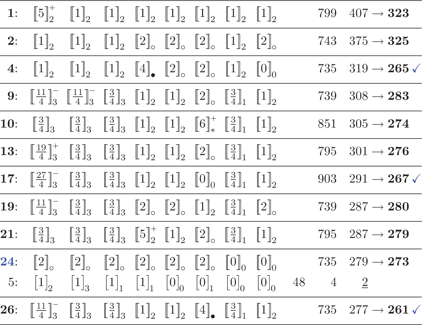
The few remaining pairs are listed in the tables below. For each vector
 $\hbar \in N$
, we show the numbers
 $|\mathfrak {F}|$
and (the ultimate “automatic” bound is typeset in boldface)
 $b^{\prime }(\mathfrak {O})\to b(\mathfrak {O})$
and list the orbits
 $\bar {\mathfrak {o}}_n$
(only those used in the computation), indicating for each the multiplicity
 $m(\bar {\mathfrak {o}}_n)$
and count
 $|\mathfrak {o}|$
and bounds
 $b^{\prime }(\mathfrak {o})\to b(\mathfrak {o})$
,
 $\mathfrak {o}\in \bar {\mathfrak {o}}_n$
. (The bounds known to be sharp are underlined.)
Convention 4.2. For the components
 $\hbar _k$
of
 $\hbar $
we use the notation
 $[\![\hbar _k^2]\!]_d$
, where d is either the discriminant class of
 $\hbar _k^2$
(in the notation of [Reference Conway and Sloane4]) or, if
 $\hbar _k\in D_k$
, the symbol
 $$ \begin{align*} 0 \mbox{ (if }\hbar_k=0\mbox{)},\quad \circ \mbox{ (if }\hbar_k^2=2\mbox{)},\quad \bullet \mbox{ (if }\hbar_k^2=4\mbox{)},\quad * \mbox{ (if }\hbar_k^2=6\mbox{)}. \end{align*} $$
If these data do not determine
 $\hbar _k$
, we use an extra superscript whose precise meaning is not very important (see [Reference Degtyarev7]).
For the components
 $l_k$
of a conic, we use the notation
 $[l_k\cdot \hbar _k]_d$
, where d and an occasional superscript have the same meaning as for
 $\hbar $
. (It is worth emphasizing that each of
 $d:=d_k$
,
 $l_k^2$
, and
 $l_k\cdot \hbar _k$
,
 $k\in \Omega $
, is constant within each combinatorial orbit
 $\mathfrak {o}$
; in the tables, we show one representative
 $\mathfrak {o}\in \bar {\mathfrak {o}}_n$
only.)
When describing partitions, in addition to
 $\mathrm {supp}\,\mathfrak {o}:=\mathrm {supp}\,l$
,
 $l\in \mathfrak {o}$
, which is also constant, we use the notation
 $$ \begin{align*} \mathcal{H}(q):=\big\{k\in\Omega\big|\hbar_k^2=q\big\},\quad q\in\mathbb{Q}, \end{align*} $$
and
 $\mathcal {H}_m(q)$
for the set of m-combinations of
 $\mathcal {H}(q)$
,
 $m\geqslant 2$
.
4.1 The lattice
$N(6\textbf {D}_4)$

There are 36 isomorphism classes of square 12 vectors
 $\hbar \in N (6\mathbf {D}_4)$
, with the maximal naïve bound
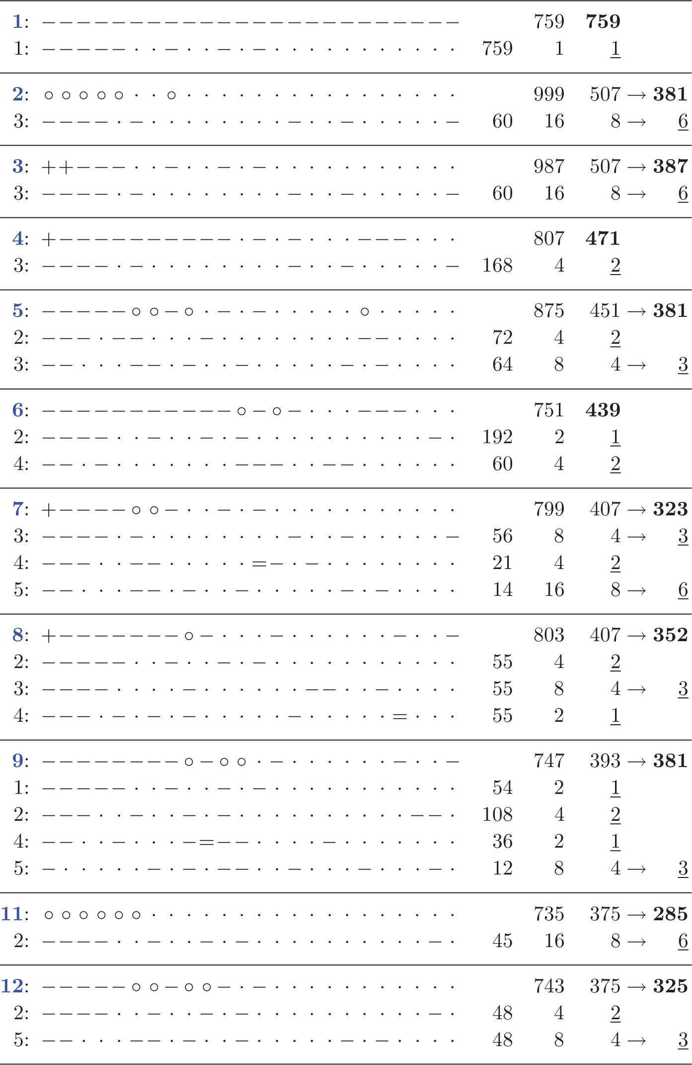
 $b(\mathfrak {O}) = 285$
(see Table 1). The only configuration with
 $b(\mathfrak {O})\geqslant 261$
is replanted (see §3.9) to #11 in
 $N(24\mathbf {A}_1)$
and is considered in §6.10 below.
The lattice
 $N(6\mathbf {D}_{4})$
.

4.2 The lattice
$N(8\textbf {A}_3)$

There are 110 isomorphism classes of square 12 vectors
 $\hbar \in N(8\textbf {A}_3)$
, with the maximal naïve bound
 $b(\mathfrak {O}) = 325$
(see Table 2). Ten of the eleven relevant configurations (those with
 $b(\mathfrak {O})\geqslant 261$
) are either replanted to other lattices or covered by Remark 3.10.
The lattice
 $N(8\mathbf {A}_{3}).$

4.2.1 Replanted configurations
The following seven configurations are replanted (see §3.9) to other lattices and, hence, considered elsewhere:
-
• #1 is replanted to #7 in
$N(24\mathbf {A}_1)$
(see §6.7); -
• #2 is replanted to #12 in
$N(24\mathbf {A}_1)$
(see §6.11); -
• #9 is replanted to #14 in
$N(12\mathbf {A}_2)$
(see §5.10); -
• #10 is replanted to #15 in
$N(12\mathbf {A}_2)$
(see §5.10); -
• #13 is replanted to #16 in
$N(12\mathbf {A}_2)$
(see §5.10); -
• #19 is replanted to #17 in
$N(12\mathbf {A}_2)$
(see §5.10); and -
• #21 is replanted to #18 in
$N(12\mathbf {A}_2)$
(see §5.10).


4.2.2 Vector 24:
we have
 $\mathcal {B}_5(\bar {\mathfrak {s}}_{\ast })= \mathcal {B}^{\prime \prime }_{11}[\bar {\mathfrak {s}}_5]= \varnothing $
; for the latter, we use the partition
 $$ \begin{align*} \mathfrak{c}_{k}:=\big\{\mathfrak{o}\subset\bar{\mathfrak{o}}_5\big|k\notin\mathrm{supp}\,\mathfrak{o}\big\}, \quad k\in\mathrm{supp}\,\,\hbar. \end{align*} $$
This case completes the proof of Theorem 4.1.
 $\square $
5 The lattice
$N(12\mathbf {A}_2)$

The goal of this section is the following theorem.
Theorem 5.1. Let
 $N:=N(12\mathbf {A}_2)$
and
 $\hbar \in N$
,
 $\hbar ^2=12$
. Then, with one exception (up to automorphism), for any geometric set
 $\mathfrak {L}\subset \mathfrak {F}(N,\hbar )$
, one has
 $|\mathfrak {L}|\leqslant 260$
. The exception is the set
 $\mathfrak {M}^{\mathrm {i}}_{285}$
of size
 $285$
, see (5.2).
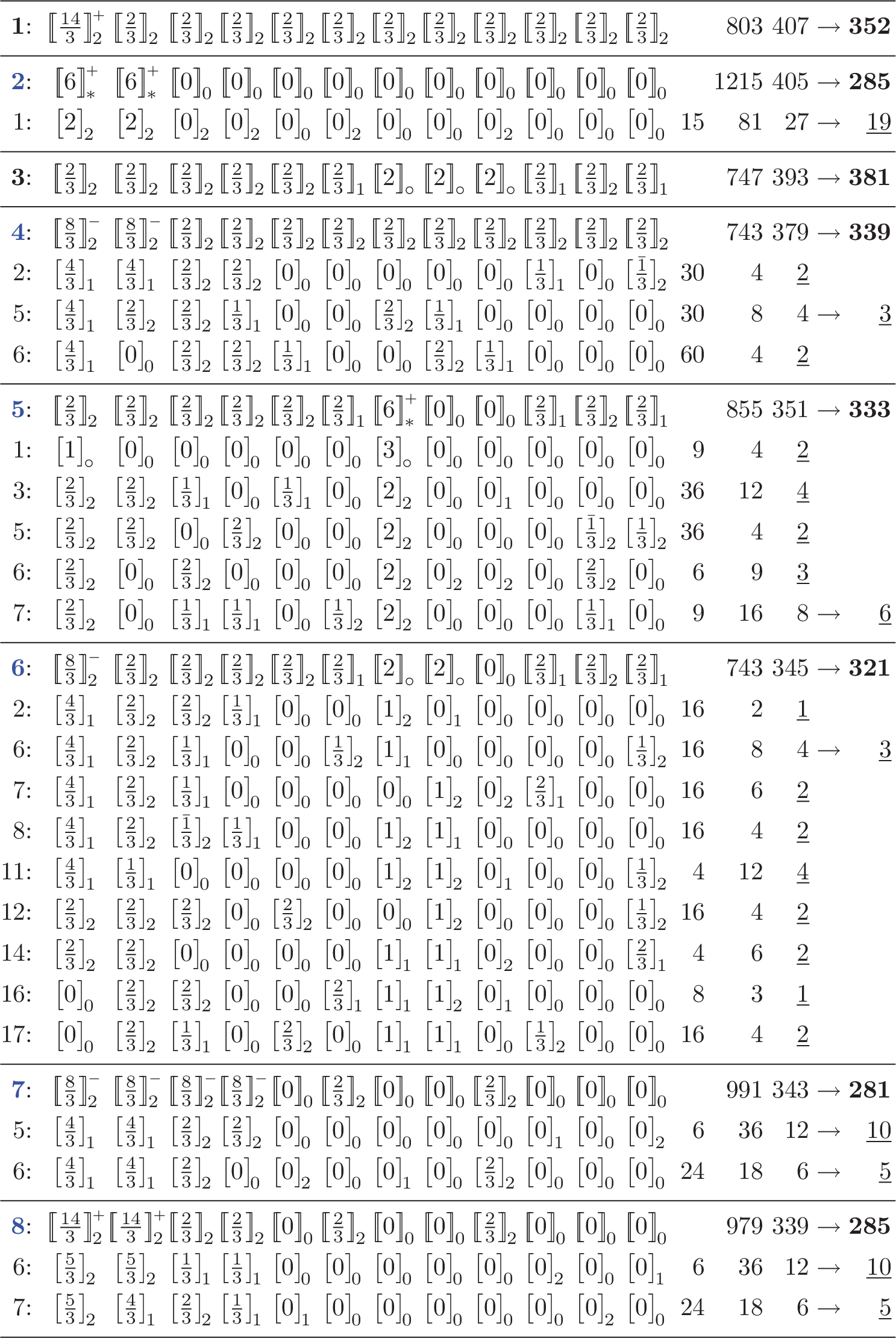
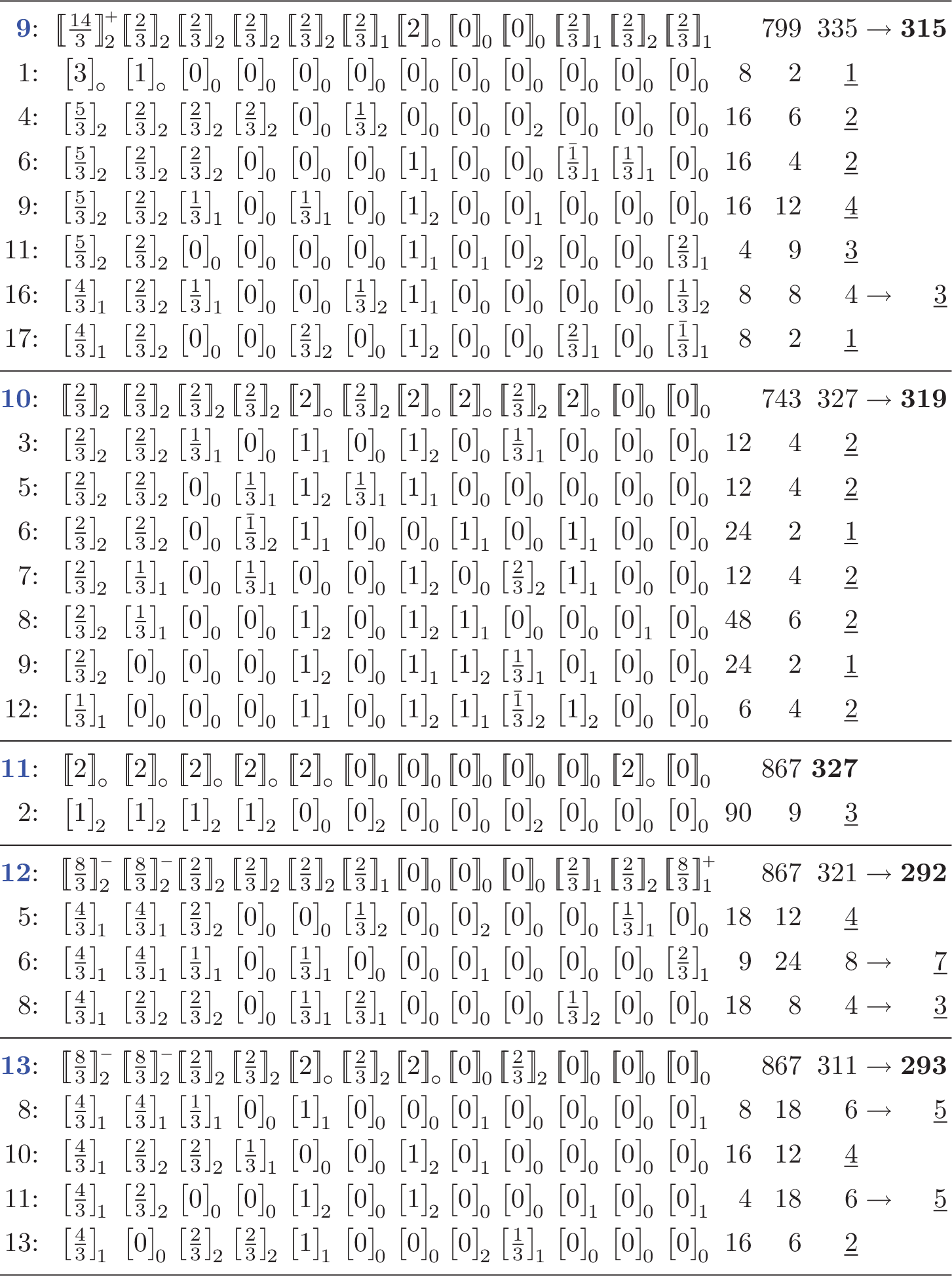
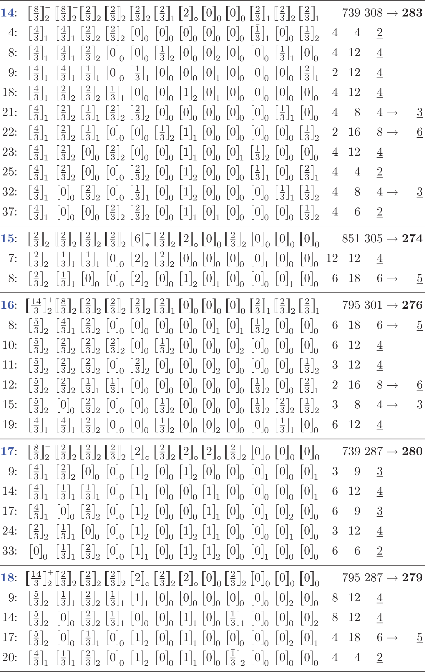
Proof. There are 29 isomorphism classes of square 12 vectors
 $\hbar \in N(12\mathbf {A}_2)$
, with the maximal naïve bound
 $b(\mathfrak {O}) = 381$
(see Tables 3–5). As above, we list only those vectors
 $\hbar $
for which
 $b(\mathfrak {O})\geqslant M$
(cf. also Remark 3.10).
The lattice
 $N(12\mathbf {A}_{2}).$

The lattice
 $N(12\mathbf {A}_{2})$
.

The lattice
 $N(12\mathbf {A}_{2})$
.

5.1 Replanted configurations
Two configurations can be replanted (see §3.9) to
 $N(24\mathbf {A}_1)$
and are considered in §6. They are as follows:


5.2 Vector 2
We have
 $|\mathrm {stab}\,\hbar |=720$
and
 $\mathrm {rk}\,\mathfrak {F}=21$
. Since the first combinatorial estimate
 $b(\mathfrak {o})\leqslant 27$
,
 $\mathfrak {o}\in \bar {\mathfrak {o}}_1$
, is too high, we use blocks (see [Reference Degtyarev7, Sec. 4.2] for details) to compute large geometric intersections
 $\mathfrak {L}\cap \mathfrak {o}$
only, arriving at
 $$ \begin{align*} |\mathfrak{L}\cap\mathfrak{o}|=19 \text{ or } |\mathfrak{L}\cap\mathfrak{o}|\leqslant15 \text{ for any }\mathfrak{o}\in\bar{\mathfrak{o}}_1 \text{ and geometric set }\mathfrak{L}\subset\mathfrak{F}. \end{align*} $$
It follows that
 $|\mathfrak {L}|\leqslant 245$
whenever
 $|\mathfrak {L}\cap \mathfrak {o}|<19$
for at least 10 orbits
 $\mathfrak {o}\in \bar {\mathfrak {o}}_1$
. Then, using patterns (see §3.4), we compute the geometric sets
 $\mathfrak {L}$
satisfying
 $|\mathfrak {L}\cap \mathfrak {o}|=19$
for (at least) six orbits
 $\mathfrak {o}\in \bar {\mathfrak {o}}_1$
. We find one set
 $\mathfrak {M}^{\mathrm {i}}_{285}$
of rank
 $20$
and size
 $285$
and one set
 $\mathfrak {L}$
of rank
 $18$
; extending the latter as in §3.6, we obtain, apart from
 $\mathfrak {M}^{\mathrm {i}}_{285}$
, five sets of sizes
 $249$
,
 $231$
,
 $213$
,
 $213$
, and
 $207$
.
The maximizing set
 $\mathfrak {M}^{\mathrm {i}}_{285}$
can be described as
 $$ \begin{align} \mathfrak{M}^{\mathrm{i}}_{285}=\mathfrak{F}\cap r^\perp,\quad r:=\sum_{k\in\Omega}(\text{a root }r_k\in\hbar_k^\perp\subset D_k\text{)}. \end{align} $$
Clearly, vectors
 $r_k\in D_k$
and r as in (5.2) are unique up to the action of
 $\mathrm {R}_\hbar $
.
Another large set worth mentioning is
 $$ \begin{align} \mathfrak{L}^{\mathrm{i}}_{249}=\mathfrak{F}\cap(r+r_k)^\perp,\quad k\in\Omega\smallsetminus\mathrm{supp}\,\hbar, \end{align} $$
where
 $r_k\in D_k$
and
 $r=\sum r_k$
are as in (5.2). This set is discussed in Example 8.4.
5.3 Vector 4
Using the partitions
 $$ \begin{align*} \begin{array}{lll} \mathfrak{c}_{k}:=\bigl\{\mathfrak{o}\in\bar{\mathfrak{o}}_2\bigm|l_k\cdot\hbar_k=-\tfrac{1}{3}\bigr\}, & k \in\mathcal{H}\bigl(\tfrac{2}{3}\bigr)&\text{(onefold)},\\ \mathfrak{c}^{\prime}_{k}:=\bigl\{\mathfrak{o}\in\bar{\mathfrak{o}}_5\bigm|l_k\cdot\hbar_k=\tfrac{2}{3}\bigr\}, &k\in\mathcal{H}\bigl(\tfrac{8}{3}\bigr) &\text{(onefold)},\\ \mathfrak{c}^{\prime\prime}_{k}:=\bigl\{\mathfrak{o}\in\bar{\mathfrak{o}}_6\bigm| l_k\cdot\hbar_k=\tfrac{1}{3}\bigr\}, & k\in\mathcal{H}\bigl(\tfrac{2}{3}\bigr) &\text{(twofold)}, \end{array} \end{align*} $$
we show that
 $\mathcal {B}^{\ast }_{24}(\bar {\mathfrak {s}}_{\ast },\bar {\mathfrak {o}}_2)= \mathcal {B}^{\prime \prime }_{19}(\bar {\mathfrak {o}}_5)= \mathcal {B}^{\prime \prime }_{33}(\bar {\mathfrak {o}}_6)= \varnothing $
.
5.4 Vector 5
Using the partitions
 $$ \begin{align*} \begin{array}{lll} \mathfrak{c}_{k}:=\bigl\{\mathfrak{o}\in\bar{\mathfrak{o}}_3\bigm|l_k\cdot\hbar_k=\tfrac{2}{3}\bigr\}, & k\in\mathcal{H}\bigl(\tfrac{2}{3}\bigr) &\text{(twofold)},\\ \mathfrak{c}^{\prime}_{k}:=\bigl\{\mathfrak{o}\in\bar{\mathfrak{o}}_5\bigm|l_k\cdot\hbar_k=-\tfrac{1}{3}\bigr\}, &k\in\mathcal{H}\bigl(\tfrac{2}{3}\bigr) &\text{(onefold)}, \end{array} \end{align*} $$
we show that
 $\mathcal {B}^{\prime \prime }_{35}(\bar {\mathfrak {o}}_3)=\varnothing $
and compute
 $\mathcal {B}^{\ast }_{18}(\bar {\mathfrak {s}}_{\ast },\bar {\mathfrak {o}}_5)$
; the latter consists of four sets of size
 $111$
,
 $99$
,
 $99$
,
 $95$
and rank
 $16$
,
 $16$
,
 $15$
,
 $16$
, respectively, which are extended by a maximal orbit (see §3.7) twice. Similarly, the only set
 $\mathfrak {L}\in \mathcal {B}^{\ast }_{17}(\bar {\mathfrak {o}}_7, \bar {\mathfrak {o}}_6, \bar {\mathfrak {o}}_1)$
has rank
 $16$
and can be extended twice by a maximal orbit. The largest set observed in this computation has size
 $249$
; letting
 $\{n\}:=\mathcal {H}(2)$
and
 $\{p,q\}:=\mathcal {H}(0)$
, this set can be described as
 $$ \begin{align} \mathfrak{L}^{\mathrm{ii}}_{249}:=\mathfrak{F}\cap\mathrm{span}\,\bigl(\hbar-2\hbar_n,r+r_p,r_n,r_q,\bigr)^\perp, \end{align} $$
where a collection of roots
 $r_k\in \hbar _k^\perp \subset D_k$
,
 $k\in \Omega $
, and vector
 $r:=\sum _{k\in \Omega }r_k$
are as in (5.2). This set is discussed in Example 8.4.
5.5 Vector 6
We have
 $$ \begin{align*} \mathcal{B}^{\ast}_{12}(\bar{\mathfrak{o}}_8,\bar{\mathfrak{o}}_{16})= \mathcal{B}^{\ast}_{12}(\bar{\mathfrak{o}}_{17}\cup \bar{\mathfrak{o}}_{14})= \mathcal{B}^{\prime\prime}_{12}(\bar{\mathfrak{s}}_{\ast},\bar{\mathfrak{o}}_{6})= \mathcal{B}^{\prime\prime}_{9}(\bar{\mathfrak{o}}_{12})= \mathcal{B}^{\prime\prime}_{3}(\bar{\mathfrak{o}}_{7})= \varnothing. \end{align*} $$
To complete the hypotheses of Lemma 3.5, we compute the set
 $\mathcal {B}^{\prime \prime }_{7}(\bar {\mathfrak {o}}_{2},\bar {\mathfrak {o}}_{11},\bar {\mathfrak {o}}_{9})=\varnothing $
employing the replanting involution
 $\bar {\tau }=(2,9)$
(see §3.9): due to the symmetry, we can assume that
 $\delta (\mathfrak {L};\bar {\mathfrak {o}}_{2})\leqslant \delta (\mathfrak {L};\bar {\mathfrak {o}}_{9})$
; hence, it suffices to consider patterns satisfying
 $\delta (\mathfrak {L};\bar {\mathfrak {o}}_{2})\leqslant 3$
at step
 $1$
and
 $2\delta (\mathfrak {L};\bar {\mathfrak {o}}_{2})+\delta (\mathfrak {L};\bar {\mathfrak {o}}_{11})\leqslant 7$
at step
 $2$
.
5.6 Vector 8
Using the partition
 $$ \begin{align*} \mathfrak{c}_{k}:=\bigl\{\mathfrak{o}\in\bar{\mathfrak{o}}_7\bigm|l_k\cdot\hbar_k=\tfrac23\bigr\},\quad k\in\mathcal{H}\bigl(\tfrac{2}{3}\bigr), \end{align*} $$
we show that
 $\mathcal {B}^{\prime \prime }_{12}(\bar {\mathfrak {o}}_7)=\varnothing $
. In addition,
 $\mathcal {B}^{\prime \prime }_{11}(\bar {\mathfrak {o}}_6)=\varnothing $
.
5.7 Vector 9
This set is reflexive (see §3.9), the replanting involution being
 $$ \begin{align*} \bar{\tau}=(1,20)(2,19)(4,13)(7,17)(8,16). \end{align*} $$
We have
 $\mathcal {B}^{\prime \prime }_{10}(\bar {\mathfrak {o}}_{6},\bar {\mathfrak {o}}_{11})=\mathcal {B}^{\prime \prime }_{15}(\bar {\mathfrak {s}}_{\ast },\bar {\mathfrak {o}}_{9})=\varnothing $
and
 $\mathcal {B}^{\prime \prime }_{5}(\bar {\mathfrak {o}}_{4})=\mathcal {B}^{\ast }_{7}(\bar {\mathfrak {o}}_{1}, \bar {\mathfrak {o}}_{17}, \bar {\mathfrak {o}}_{16})=\varnothing $
; from the latter, applying
 $\bar {\tau }$
, we derive that also
 $\mathcal {B}^{\prime \prime }_{5}(\bar {\mathfrak {o}}_{13})=\mathcal {B}^{\ast }_{7}(\bar {\mathfrak {o}}_{20},\bar {\mathfrak {o}}_{7},\bar {\mathfrak {o}}_{8})=\varnothing $
.
5.8 Vector 10
We have
 $\mathcal {B}^{\prime \prime }_{5}(\bar {\mathfrak {o}}_{5},\bar {\mathfrak {o}}_{12})= \mathcal {B}^{\ast }_8(\bar {\mathfrak {o}}_{3},\bar {\mathfrak {o}}_{6})= \mathcal {B}^{\ast }_8(\bar {\mathfrak {o}}_{7},\bar {\mathfrak {o}}_{9})= \varnothing $
. Then, using the partition
 $$ \begin{align*} \mathfrak{c}_{k}:=\bigl\{\mathfrak{o}\in\bar{\mathfrak{o}}_8\bigm|k\notin\mathrm{supp}\,\mathfrak{o}\bigr\},\quad k\in\mathcal{H}(2), \end{align*} $$
we show that
 $\mathcal {B}^{\prime \prime }_{15}(\bar {\mathfrak {o}}_{8})=\varnothing $
and
 $\delta (\mathfrak {L};\bar {\mathfrak {o}}_{8})>34$
for each
 $\mathfrak {L}\in \mathcal {B}^{\prime \prime }_{18}(\bar {\mathfrak {s}}_{\ast })$
.
5.9 Vector 11
We have
 $ \mathcal {B}_17(\bar {\mathfrak {s}}_{\ast })= \mathcal {B}^{\prime \prime }_{48}(\bar {\mathfrak {o}}_{2})= \varnothing $
; for
 $\bar {\mathfrak {o}}_2$
, we use the partition
 $$ \begin{align*} \mathfrak{c}_{c}:=\bigl\{\mathfrak{o}\in\bar{\mathfrak{o}}_{2}\bigm|c\subset\mathrm{supp}\,\mathfrak{o}\bigr\},\quad c\in\mathcal{H}_2(0). \end{align*} $$
5.10 Other configurations
For the remaining eight vectors
 $\hbar \in N$
, we directly use patterns to compute a few sets of the form
 $\mathcal {B}^{\prime \prime }_d(\mathfrak {C})$
and refer to Lemma 3.5.
-
#7:
$\mathcal {B}^{\prime \prime }_{11}(\bar {\mathfrak {o}}_{5})= \mathcal {B}^{\prime \prime }_{8}(\bar {\mathfrak {o}}_{6})= \varnothing $
; -
#12:
$\mathcal {B}^{\prime \prime }_{15}(\bar {\mathfrak {o}}_{5})= \mathcal {B}^{\prime \prime }_{9}(\bar {\mathfrak {o}}_{6})= \mathcal {B}^{\prime \prime }_{5}(\bar {\mathfrak {o}}_{8})= \varnothing $
; -
#13:
$\mathcal {B}^{\prime \prime }_{13}(\bar {\mathfrak {o}}_{10})= \mathcal {B}^{\prime \prime }_{8}(\bar {\mathfrak {o}}_{8}\cup \bar {\mathfrak {o}}_{11})= \mathcal {B}^{\ast }_{9}(\bar {\mathfrak {s}}_{\ast },\bar {\mathfrak {o}}_{13})= \varnothing $
; -
#14:
$\mathcal {B}^{\prime \prime }_{5}(\bar {\mathfrak {o}}_{18}, \bar {\mathfrak {o}}_{22}, \bar {\mathfrak {o}}_{4})= \mathcal {B}^{\prime \prime }_{5}(\bar {\mathfrak {o}}_{8}, \bar {\mathfrak {o}}_{25}, \bar {\mathfrak {o}}_{37})= \mathcal {B}^{\prime \prime }_{5}(\bar {\mathfrak {o}}_{23}, \bar {\mathfrak {o}}_{32})= \mathcal {B}^{\ast }_{4}(\bar {\mathfrak {s}}_{\ast }, \bar {\mathfrak {o}}_{21}, \bar {\mathfrak {o}}_{9})= \varnothing $
; -
#15:
$\mathcal {B}^{\prime \prime }_{9}(\bar {\mathfrak {o}}_{7})= \mathcal {B}^{\prime \prime }_{4}(\bar {\mathfrak {o}}_{8})= \varnothing $
; -
#16:
$\mathcal {B}^{\prime \prime }_{5}(\bar {\mathfrak {o}}_{10}, \bar {\mathfrak {o}}_{11})= \mathcal {B}^{\prime \prime }_{4}(\bar {\mathfrak {o}}_{19}, \bar {\mathfrak {o}}_{12})= \mathcal {B}^{\prime \prime }_{4}(\bar {\mathfrak {o}}_{15}, \bar {\mathfrak {o}}_{8})= \varnothing $
; -
#17:
$\mathcal {B}^{\prime \prime }_{6}(\bar {\mathfrak {o}}_{14}, \bar {\mathfrak {o}}_{24})= \mathcal {B}^{\ast }_{12}(\bar {\mathfrak {s}}_{\ast }, \bar {\mathfrak {o}}_{17}, \bar {\mathfrak {o}}_{33}, \bar {\mathfrak {o}}_{9})= \varnothing $
; -
#18:
$\mathcal {B}^{\prime \prime }_{5}(\bar {\mathfrak {o}}_{14}, \bar {\mathfrak {o}}_{20})= \mathcal {B}^{\prime \prime }_{5}(\bar {\mathfrak {s}}_{\ast }, \bar {\mathfrak {o}}_{17})= \mathcal {B}_{7}(\bar {\mathfrak {o}}_{9})= \varnothing $
.


This completes the proof of Theorem 5.1.
 $\square $
6 The lattice
$N(24\mathbf {A}_{1})$

The goal of this section is the following theorem.
Theorem 6.1. Let
 $N:=N(24\mathbf {A}_1)$
and
 $\hbar \in N$
,
 $\hbar ^2=12$
. Then, with few exceptions, one has
 $|\mathfrak {L}|\leqslant 260$
for any geometric set
 $\mathfrak {L}\subset \mathfrak {F}(N,\hbar )$
. Up to automorphism, there are six exceptional sets:
-
• three sets
$\mathfrak {M}^{\mathrm {ii}}_{285}$
,
$\mathfrak {M}^{\mathrm {iii}}_{285}$
,
$\mathfrak {M}^{\mathrm {iv}}_{285}$
of size
$285$
, see (6.3), (6.4), and (6.6), and -
• three sets
$\mathfrak {G}^{\mathrm {i}}_{261}$
,
$\mathfrak {G}^{\mathrm {ii}}_{261}$
,
$\mathfrak {G}^{\mathrm {iii}}_{261}$
of size
$261$
, see (6.2), (6.5), and (6.7).


Proof. There are 13 isomorphism classes of square 12 vectors
 $\hbar \in N(24\mathbf {A}_1)$
, with the maximal naïve bound
 $b(\mathfrak {O}) = 759$
(see Table 6). (As above, we list only those vectors
 $\hbar $
for which
 $b(\mathfrak {O})\geqslant M$
, cf. also Remark 3.10.) To save space, we fix a root basis
 $\{r_k\}$
,
 $k\in \Omega $
, for
 $D=24\mathbf {A}_1$
and, given a vector
 $v\in N$
(either
 $\hbar $
or a conic l), use the following notation for its components
 $v_k=\alpha r_k\in D_k^\vee $
:
 $$ \begin{align*} \cdot \mbox{ (}\alpha=0\mbox{)},\quad - \mbox{ or }= \mbox{ (}\alpha=\pm\frac{1}{2}\mbox{)},\quad \circ \mbox{ (}\alpha=\pm1\mbox{)},\quad + \mbox{ (}\alpha=\pm\frac{3}{2}\mbox{)},\quad \bullet \mbox{ (}\alpha=\pm2\mbox{)}. \end{align*} $$
Here,
 $=$
is used only for
 $l_k$
and only if
 $\hbar _k\cdot l_k<0$
; in all other cases, the signs of
 $l_k$
and
 $\hbar _k$
agree, so that we have
 $\hbar _k\cdot l_k\geqslant 0$
.
The lattice
 $N(24\mathbf {A}_{1})$
.

Recall that the kernel
 $$ \begin{align*} N\bmod24\mathbf{A}_2\subset\mathrm{discr}(24\mathbf{A}_1)\cong(\mathbb{Z}/2)^{24} \end{align*} $$
of the extension
 $N\supset 24\mathbf {A}_1$
is the extended binary Golay code
 $\mathcal {C}_{24}$
(see [Reference Conway and Sloane4]). The map
 $\mathrm {supp}\,\:\mathrm {discr}(24\mathbf {A}_1)\to (\text {the power set of }\Omega )$
identifies codewords with subsets of
 $\Omega $
; then,
 $\mathcal {C}_{24}$
is invariant under complement and, in addition to
 $\varnothing $
and
 $\Omega $
, it consists of
 $759$
octads,
 $759$
complements thereof, and
 $2576$
dodecads.
To simplify the notation, we identify the basis vectors
 $r_k$
(which are assumed fixed throughout) with their indices
 $k\in \Omega $
. For a subset
 $\mathcal {S}\subset \Omega $
, we let
 $\bar {1}_{\mathcal {S}}:=\sum r$
,
 $r\in \mathcal {S}$
, and we abbreviate
 $[\mathcal {S}]:=\frac {1}{2}\bar {1}_{\mathcal {S}}\in N$
if
 $\mathcal {S}\in \mathcal {C}_{24}$
is a codeword.
Now, as in the previous proofs, we treat the configurations one by one. We also give a more detailed description of each vector
 $\hbar $
in terms of the Golay code
 $\mathcal {C}_{24}$
.

6.2 Vector 2
We have
 $|\mathrm {stab}\,\hbar |=11,520$
and
 $\hbar =\bar {1}_{\mathcal {R}}$
, where
 $|\mathcal {R}|=6$
and
 $\mathcal {R}$
is a subset of an octad
 $\mathcal {O}:=\mathcal {R}\cup \{r_1,r_2\}\in \mathcal {C}_{24}$
(cf. §6.10). Using the partition
 $$ \begin{align*} \mathfrak{c}_{c}:=\bigl\{\mathfrak{o}\in\bar{\mathfrak{o}}_3\bigm|c\cap\mathrm{supp}\,\mathfrak{o}=\varnothing\bigr\},\quad c\in\mathcal{H}_2(0), \end{align*} $$
we show that
 $\mathcal {B}^{\prime \prime }_{120}(\bar {\mathfrak {s}}_{\ast },\bar {\mathfrak {o}}_{3})=\varnothing $
. There is but one discarded set,
 $\mathfrak {G}^{\mathrm {i}}_{261}$
of size
 $261$
, that satisfies the threshold (3.4); this set can be described as
 $$ \begin{align} \mathfrak{G}^{\mathrm{i}}_{261}= \mathfrak{F}\cap\mathrm{span}\,\bigl(\hbar-4[o],[\Omega\smallsetminus\mathcal{O}],r_1,r_2\bigr)^\perp, \end{align} $$
where
 $|o|=8$
,
 $|o\cap \mathcal {O}|=4$
,
 $r_1\in o$
,
 $r_2\notin o$
. (Till the end of this section, we reserve the notation o for a codeword,
 $o\in \mathcal {C}_{24}$
, intersecting the other fixed sets in a certain prescribed way. In each case, one can easily check that the set of extra data used in the description of an extremal geometric set is unique up to
 $\mathrm {stab}\,\hbar $
.)
6.3 Vector 3
We have
 $|\mathrm {stab}\,\hbar |=11,520$
and
 $\hbar =[\mathcal {O}]+\bar {1}_{\mathcal {R}}$
, where
 $\mathcal {O}$
is an octad and
 $\mathcal {R}:=\{r_1,r_2\}\subset \mathcal {O}$
is a two-element set. Note that
 $\mathrm {rk}\,\mathfrak {F}=23$
, as
 $\mathfrak {F}$
is annihilated by
 $[\mathcal {O}]-\bar {1}_{\mathcal {R}}$
; this configuration can be re-embedded as #2, acquiring a few extra conics (increasing the rank to
 $24$
) and a few extra roots orthogonal to
 $\hbar $
(changing the combinatorial orbits). Using the partition
 $$ \begin{align*} \mathfrak{c}_{c}:=\bigl\{\mathfrak{o}\in\bar{\mathfrak{o}}_3\bigm|c\subset\mathrm{supp}\,\mathfrak{o}\bigr\},\quad c\in\mathcal{H}_2\bigl(\tfrac{1}{2}\bigr), \end{align*} $$
we show that
 $\mathcal {B}^{\prime \prime }_{126}(\bar {\mathfrak {s}}_{\ast },\bar {\mathfrak {o}}_{3})=\varnothing $
. Three of the discarded sets satisfy (3.4); they are of the form
 $$ \begin{align*} \mathfrak{L}=\mathfrak{F}\cap\mathrm{span}\,\bigl(\hbar-4r_1,\hbar-4r_2,[\Omega\smallsetminus\mathcal{O}],v\bigr)^\perp, \end{align*} $$
where the fourth vector v is as follows:
 $$ \begin{align} \kern4pt\mathfrak{M}^{\mathrm{ii}}_{285}:\quad v=s, \qquad\qquad\qquad\kern-2pt s\in\Omega\smallsetminus\mathcal{O}, \qquad\qquad\qquad\qquad\qquad\qquad\quad \end{align} $$
 $$ \begin{align} \kern-3pt \mathfrak{M}^{\mathrm{iii}}_{285}:\quad&v=[{o}]-r_1,\ && |o|=8,\ |o\cap\mathcal{O}|=2,&\quad& r_1\in o,\ r_2\in o, \end{align} $$
 $$ \begin{align} \mathfrak{G}^{\mathrm{ii}}_{261}:\quad&v=[{o}]-r_1,\ && |o|=8,\ |o\cap\mathcal{O}|=4,&\quad& r_1\in o,\ r_2\notin o. \end{align} $$
As above,
 $o\in \mathcal {C}_{24}$
and the subscript in the notation refers to the cardinality.
6.4 Vector 4
We have
 $|\mathrm {stab}\,\hbar |=20160$
and
 $\hbar =[\mathcal {O}]+r$
, where
 $\mathcal {O}$
is a codeword of length
 $16$
and
 $r\in \mathcal {O}$
. Using the (mega-)clusters
 $$ \begin{align*} \mathfrak{c}_{c}:=\bigl\{\mathfrak{o}\in\bar{\mathfrak{o}}_3\bigm|c\subset\mathrm{supp}\,\mathfrak{o}\bigr\},\quad \mathfrak{m}_{k}:=\bigl\{\mathfrak{c}{c}\bigm|c\ni k\bigr\},\quad k\in\mathcal{H}(0),\ c\in\mathcal{H}_2(0), \end{align*} $$
we show that
 $\mathcal {B}^{\prime \prime }_{124}(\bar {\mathfrak {o}}_{3})=\varnothing $
and
 $\delta (\mathfrak {L};\bar {\mathfrak {o}}_{3})>210$
for each set
 $\mathfrak {L}\in \mathcal {B}^{\prime \prime }_{85}(\bar {\mathfrak {s}}_{\ast })$
. Two of the discarded sets satisfy the threshold (3.4); they are of the form
 $$ \begin{align*} \mathfrak{L}=\mathfrak{F}\cap\mathrm{span}\,\bigl(\hbar-4r,[\Omega\smallsetminus\mathcal{O}],s,v\bigr)^\perp, \end{align*} $$
where
 $s\in \Omega \smallsetminus \mathcal {O}$
and the fourth vector v is as follows:
 $$ \begin{align} \mathfrak{M}^{\mathrm{iv}}_{285} &:\quad v=t,\qquad\quad\ t\in\Omega\smallsetminus\mathcal{O},\ t\ne s,\quad\quad\quad\quad\quad\quad\quad\quad \end{align} $$
 $$ \begin{align} \mathfrak{M}^{\mathrm{iii}}_{285}&:\quad v=[{o}]-r,\quad |o|=\phantom{0}8,\ |o\cap\mathcal{O}|=4,\quad r\in o,\ s\notin o, \end{align} $$
 $$ \begin{align} \kern3.5pt\mathfrak{L}^{\mathrm{ii}}_{261} &:\quad v=[{o}]-r,\quad |o|=12,\ |o\cap\mathcal{O}|=6,\quad r\notin o,\ s\notin o. \end{align} $$
The third set
 $\mathfrak {L}^{\mathrm {iii}}_{249}$
is discussed in Example 8.4.
6.5 Vector 5
We have
 $|\mathrm {stab}\,\hbar |=2304$
and
 $\hbar =[\mathcal {O}]+\bar {1}_{\mathcal {R}}$
, where
 $\mathcal {O}$
is an octad and
 $\mathcal {R}\subset \Omega \smallsetminus \mathcal {O}$
is a four-element set such that there is an octad
 $o\supset \mathcal {R}$
with the property
 $|o\cap \mathcal {O}|=4$
(cf. §6.11). Using the partitions
 $$ \begin{align*} \mathfrak{c}_{c}&:=\bigl\{\mathfrak{o}\in\bar{\mathfrak{o}}_2\bigm|c\subset\mathrm{supp}\,\mathfrak{o}\bigr\},\quad c\in\mathcal{H}_2(2),\\ \mathfrak{c}^{\prime}_{k}&:=\bigl\{\mathfrak{o}\in\bar{\mathfrak{o}}_3\bigm|k\notin\mathrm{supp}\,\mathfrak{o}\bigr\},\quad k \in\mathcal{H}(2), \end{align*} $$
we show
 $\mathcal {B}^{\prime \prime }_{53}(\bar {\mathfrak {o}}_{2})=\mathcal {B}^{\prime \prime }_{51}[\bar {\mathfrak {o}}_{3}]=\varnothing $
and
 $\delta [\mathfrak {L};\bar {\mathfrak {o}}_{3}]>66$
for each set
 $\mathfrak {L}\in \mathcal {B}^{\prime \prime }_{14}(\bar {\mathfrak {s}}_{\ast })$
.
6.6 Vector 6
We have
 $|\mathrm {stab}\,\hbar |=11520$
and
 $\hbar =[\mathcal {O}]+\bar {1}_{\mathcal {R}}$
, where
 $\mathcal {O}$
is a codeword of length
 $16$
and
 $\mathcal {R}\subset \Omega \smallsetminus \mathcal {O}$
is a
 $2$
-element set. Using the (mega-)clusters
 $$ \begin{align*} \mathfrak{c}_{k,n}&:=\bigl\{\mathfrak{o}\in\bar{\mathfrak{o}}_2\bigm|k,n\in\mathrm{supp}\,\mathfrak{o}\bigr\},\quad \mathfrak{m}_{k} :=\bigl\{\mathfrak{c}{k,n}\bigr\},\qquad\kern8pt k\in\mathcal{H}(0),\ n \in\mathcal{H}(2),\\ \mathfrak{c}^{\prime}_{c}&:=\bigl\{\mathfrak{o}\in\bar{\mathfrak{o}}_4\bigm|c\subset\mathrm{supp}\,\mathfrak{o}\bigr\},\qquad \mathfrak{m}^{\prime}_{k}:=\bigl\{\mathfrak{c}^{\prime}_{c}\bigm|c\ni k\bigr\},\quad k \in\mathcal{H}(0),\ c\in\mathcal{H}_2(0), \end{align*} $$
we show that
 $\mathcal {B}^{\prime \prime }_{47}(\bar {\mathfrak {o}}_{2})=\mathcal {B}^{\prime \prime }_{49}(\bar {\mathfrak {o}}_{4})=\varnothing $
and
 $\delta (\mathfrak {L};\bar {\mathfrak {o}}_{4})>130$
for each set
 $\mathfrak {L}\in \mathcal {B}^{\prime \prime }_{80}(\bar {\mathfrak {s}}_{\ast })$
.
6.7 Vector 7
We have
 $|\mathrm {stab}\,\hbar |=336$
and
 $\hbar =[\mathcal {O}]+\bar {1}_{\mathcal {R}}+r$
, where
 $\mathcal {O}\ni r$
is an octad and
 $\mathcal {R}\subset \Omega \smallsetminus \mathcal {O}$
is a two-element set. Using the partition
 $$ \begin{align*} \mathfrak{c}_{k}:=\bigl\{\mathfrak{o}\in\bar{\mathfrak{o}}_3\bigm|c\in\mathrm{supp}\,\mathfrak{o}\bigr\},\quad k\in\mathcal{H}(2), \end{align*} $$
we show that
 $\mathcal {B}^{\prime \prime }_{15}(\bar {\mathfrak {o}}_{3})=\varnothing $
. Besides,
 $\mathcal {B}^{\prime \prime }_{5}(\bar {\mathfrak {o}}_{4})=\mathcal {B}^{\prime \prime }_{40}(\bar {\mathfrak {s}}_{\ast },\bar {\mathfrak {o}}_{5})=\varnothing $
.
6.8 Vector 8
We have
 $|\mathrm {stab}\,\hbar |=660$
and
 $\hbar =[\mathcal {O}]+r+s$
, where
 $\mathcal {O}\ni r$
is a dodecad and
 $s\in \Omega \smallsetminus \mathcal {O}$
. Using the partitions
 $$ \begin{align*} \mathfrak{c}_{k}&:=\bigl\{\mathfrak{o}\in\bar{\mathfrak{o}}_2\bigm|k\in\mathrm{supp}\,\mathfrak{o}\bigr\},\qquad\!\!\! k\in\mathcal{H}(0) \quad \, \mbox{(twofold)},\\ \mathfrak{c}^{\prime}_{k}&:=\bigl\{\mathfrak{o}\in\bar{\mathfrak{o}}_3\bigm|k\in\mathrm{supp}\,\mathfrak{o}\bigr\},\qquad\!\!\! k\in\mathcal{H}(0)\quad \, \mbox{(threefold)},\\ \mathfrak{c}^{\prime\prime}_{k}&:=\bigl\{\mathfrak{o}\in\bar{\mathfrak{o}}_4\bigm|l_k\cdot\hbar_k=-\tfrac{1}{2}\bigr\}, \quad k\in\mathcal{H}\bigl(\tfrac{1}{2}\bigr)\quad \!\mbox{(onefold)}, \end{align*} $$
we show that
 $\mathcal {B}^{\prime \prime }_{38}(\bar {\mathfrak {o}}_{2})=\mathcal {B}^{\prime \prime }_{40}(\bar {\mathfrak {o}}_{3})=\mathcal {B}^{\prime \prime }_{11}(\bar {\mathfrak {s}}_{\ast },\bar {\mathfrak {o}}_{4})=\varnothing $
.
6.9 Vector 9
We have
 $|\mathrm {stab}\,\hbar |=432$
and
 $\hbar =[\mathcal {O}]+\bar {1}_{\mathcal {R}}$
, where
 $\mathcal {O}$
is a dodecad and
 $\mathcal {R}\subset \Omega \smallsetminus \mathcal {O}$
is a
 $3$
-element set. Using the partitions
 $$ \begin{align*} \mathfrak{c}_{k}&:=\bigl\{\mathfrak{o}\in\bar{\mathfrak{o}}_1\bigm|k\in\mathrm{supp}\,\mathfrak{o}\bigr\},\qquad\qquad\quad \quad\kern1pt k\in\mathcal{H}(2)\qquad\qquad\quad \ \kern1.8pt \mbox{(onefold)},\\ \mathfrak{c}^{\prime}_{k,n}&:=\bigl\{\mathfrak{o}\in\bar{\mathfrak{o}}_2\bigm| k\in\mathrm{supp}\,\mathfrak{o},\ n\notin\mathrm{supp}\,\mathfrak{o}\bigr\},\quad k\in\mathcal{H}(0),\ n\in\mathcal{H}(2)\quad \mbox{(twofold)}, \end{align*} $$
and, grouping the latter into mega-clusters
 $\mathfrak {m}^{\prime }_{k}:=\{\mathfrak {c}^{\prime }_{k,n}\}$
,
 $k\in \mathcal {H}(0)$
, we use patterns to show that
 $\mathcal {B}^{\prime \prime }_{13}(\bar {\mathfrak {o}}_{1})=\mathcal {B}^{\prime \prime }_{72}(\bar {\mathfrak {o}}_{2})=\varnothing $
and
 $\delta (\mathfrak {L};\bar {\mathfrak {o}}_{2})>93$
for each set
 $\mathfrak {L}\in \mathcal {B}^{\prime \prime }_{20}(\bar {\mathfrak {s}}_{\ast })$
. In addition, we have
 $\mathcal {B}^{\prime \prime }_{3}(\bar {\mathfrak {o}}_{4})=\mathcal {B}^{\prime \prime }_{8}(\bar {\mathfrak {o}}_{5})=\varnothing $
.
6.10 Vector 11
We have
 $|\mathrm {stab}\,\hbar |=2160$
and
 $\hbar =\bar {1}_{\mathcal {R}}$
, where
 $|\mathcal {R}|=6$
and
 $\mathcal {R}$
is not a subset of an octad (cf. §6.2). Using the partition
 $$ \begin{align*} \mathfrak{c}^{\prime}_{k}:=\bigl\{\mathfrak{o}\in\bar{\mathfrak{o}}_2\bigm|k\notin\mathrm{supp}\,\mathfrak{o}\bigr\},\quad k\in\mathcal{H}(2)\quad\text{(twofold)}, \end{align*} $$
we show that
 $\mathcal {B}^{\prime \prime }_{24}(\bar {\mathfrak {o}}_{2})=\varnothing $
.
6.11 Vector 12
We have
 $|\mathrm {stab}\,\hbar |=192$
and
 $\hbar =[\mathcal {O}]+\bar {1}_{\mathcal {R}}$
, where
 $\mathcal {O}$
is an octad and
 $\mathcal {R}\subset \Omega \smallsetminus \mathcal {O}$
is a four-element set such that there is no octad
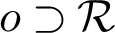 $o\supset \mathcal {R}$
with the property
 $|o\cap \mathcal {O}|=4$
(cf. §6.5). Using the partitions
 $$ \begin{align*} \mathfrak{c}_{c}&:=\bigl\{\mathfrak{o}\in\bar{\mathfrak{o}}_2\bigm|c\subset\mathrm{supp}\,\mathfrak{o}\bigr\},\quad c\in\mathcal{H}_2(2),\\ \mathfrak{c}^{\prime}_{k}&:=\bigl\{\mathfrak{o}\in\bar{\mathfrak{o}}_5\bigm|k\notin\mathrm{supp}\,\mathfrak{o}\bigr\},\quad k\in\mathcal{H}(2), \end{align*} $$
we show that
 $\mathcal {B}^{\prime \prime }_{32}(\bar {\mathfrak {s}}_{\ast },\bar {\mathfrak {o}}_{2})=\mathcal {B}^{\prime \prime }_{31}(\bar {\mathfrak {o}}_{5})=\varnothing $
.
This case concludes the proof of Theorem 6.1.
 $\square $
7 The Leech lattice
$\Lambda $
(cf. [Reference Degtyarev, Itenberg and Ottem8])

The last lattice to be considered is the root-free Leech lattice
 $\Lambda $
.
Theorem 7.1. With two exceptions (up to automorphism), one has
 $|\mathfrak {L}|\leqslant 260$
for any square
 $12$
vector
 $\hbar \in \Lambda $
and any geometric set
 $\mathfrak {L}\subset \mathfrak {F}(\Lambda ,\hbar )$
. The exceptions are:


Proof. According to Theorem 28 in [Reference Conway and Sloane4, Chap. 10], any nonzero class
 $[\hbar ]\in \Lambda /2\Lambda $
is represented by a unique pair
 $\pm a\in \Lambda $
, where
 $a^2\in \{4,6\}$
or
 $a^2=8$
and a is an element of a fixed coordinate frame. Since
 $a^2=\hbar ^2\bmod 4$
and
 $\Lambda $
is positive definite and root free, for
 $\hbar ^2=12$
, we have (up to a basis change in
 $\mathbb {Z}a+\mathbb {Z}b$
) either
-
1.
$\hbar = a + 2b$
, where
$a^2 = b^2 = 4$
and
$a \cdot b = -2$
(type
$6_{22}$
in [Reference Conway and Sloane4]) or -
2.
$\hbar = a + 2b$
, where
$a^2= 8$
,
$b^2 = 4$
, and
$a \cdot b = -3$
(type
$6_{32}$
in [Reference Conway and Sloane4])


In addition, a pair
 $a,b\in \Lambda $
as in item (1) or (2) is unique up to
 $\mathrm {O}(\Lambda )$
. Thus, there are two
 $\mathrm {O}(\Lambda )$
-orbits of square
 $12$
vectors
 $\hbar \in \Lambda $
(see Theorem 29 in [Reference Conway and Sloane4])
In each case, there is a unique orbit
 $\bar {\mathfrak {o}}_1$
and, obviously, all combinatorial orbits are single,
 $\mathfrak {O}=\bar {\mathfrak {s}}_{\ast }$
; therefore, we proceed as in §3.8, computing iterated index
 $2$
subgroups and trying to find large subsets
 $\mathfrak {L}\subset \mathfrak {F}$
of rank
 $\mathrm {rk}\,\mathfrak {L}\leqslant 20$
.
7.1 Vector 1:
$\boldsymbol{\hbar =} a \bmod 2\Lambda $
,
$a^2=4$


Let
 $F:=\mathrm {span}_{\mathbb {Z}}\mathfrak {F}$
. Then,
 $$ \begin{align*} |\mathrm{O}_\hbar(F)|=55180984320,\qquad |\mathfrak{F}|=891,\qquad \mathrm{rk}\,F=23,\qquad \mathrm{discr}\,F=\mathcal{U}\oplus\bigl\langle \tfrac{7}{4}\bigr\rangle , \end{align*} $$
and all index
 $8$
extensions of
 $F\oplus \mathbb {Z} a$
,
 $a^2=4$
, are isomorphic and have vector
 $\hbar $
of the same type 1. Note that F is not primitive in
 $\Lambda $
and
 $\mathrm {O}_\hbar (\Lambda )$
induces an index
 $6$
subgroup of
 $\mathrm {O}_\hbar (F)$
. To reduce the number of intermediate classes, we work with the smaller lattice F and larger symmetry group
 $\mathrm {O}_\hbar (F)$
; then, for each set
 $\mathfrak {L}\subset \mathfrak {F}$
found, we analyze the lattice
 $S:=\mathrm {span}\,\mathfrak {L}\cap F$
itself as well as all abstract finite index extensions
 $\bar S\supset S$
.
The computation results in four saturated sets
 $\mathfrak {L}\subset \mathfrak {F}$
of rank
 $\mathrm {rk}\,\mathfrak {L}\leqslant 20$
and size
 $|\mathfrak {L}|\geqslant 261$
: their sizes are
 $297$
,
 $285$
,
 $279$
, and
 $261$
. None of the lattices S as above has a nontrivial root-free finite index extension
 $\bar S\supset S$
satisfying
 $\hbar \in \bar S^\vee $
, and only the two sets as in the statement of Theorem 7.1 are geometric. These two sets can be described in terms of square
 $4$
vectors in
 $\Lambda $
. To this end, consider the lattice
 $U:=\mathbb {Z} a+\mathbb {Z} b+\mathbb {Z} c+\mathbb {Z} d$
with the Gram matrix
 $$ \begin{align*} \left[\begin{array}{c@{\quad}c@{\quad}c@{\quad}c} 4&-2& 1& 1\\ -2& 4&-2& 1\\ 1&-2& 4&-2\\ 1& 1&-2& 4 \end{array}\right] \end{align*} $$
and let
 $V:=U+\mathbb {Z} v$
,
 $v^2=4$
, be its extension such that
 $v\cdot a=v\cdot b=0$
and the other two products are as follows:
 $$ \begin{align} &v\cdot c=0,\quad v\cdot d=2\quad \mbox{for }\mathfrak{M}^{\mathrm{v}}_{285}, \end{align} $$
 $$ \begin{align} &v\cdot c=1,\quad v\cdot d=1\quad \mbox{for }\mathfrak{G}^{\mathrm{iv}}_{261}. \end{align} $$
Up to
 $\mathrm {O}_\hbar (\Lambda )$
, there is a unique isometry
 $V\hookrightarrow \Lambda $
such that
 $a+2b\mapsto \hbar $
, and the set in question is
 $$ \begin{align*} \mathfrak{F}(\hbar)\cap\bigl((\mathbb{Z}\hbar\oplus V^\perp)\otimes\mathbb{Q}\bigr). \end{align*} $$
Remark 7.4. The other two large sets can also be described in a similar manner. For the largest one, we can take
 $v\cdot a=v\cdot c=1$
and
 $v\cdot b=v\cdot d=-2$
, whereas for the set of size
 $279$
the whole Gram matrix should be modified.
7.2 Vector 2:
$\boldsymbol{\hbar =} a\bmod 2\Lambda $
,
$a^2=8$


Letting, as above,
 $F:=\mathrm {span}_{\mathbb {Z}}\mathfrak {F}$
, we have
 $$ \begin{align*} \mathrm{O}_\hbar(\Lambda)=\mathrm{O}_\hbar(F)=M_{24},\qquad |\mathfrak{F}|=759,\qquad \mathrm{rk}\,F=24. \end{align*} $$
Enumerating iterated index
 $2$
subgroups, we find that each subset
 $\mathfrak {L}\subset \mathfrak {F}$
of size
 $|\mathfrak {L}|\geqslant 261$
has rank
 $\mathrm {rk}\,\mathfrak {L}\geqslant 21$
and, therefore, is not geometric.
8 Proofs and examples
In this concluding section we complete the proof of Theorem 1.1 and discuss a few interesting examples discovered in the course of the computation.
8.1 Proof of Theorem 1.1
By Theorem 2.1 (and the Riemann–Roch theorem), maximal (with respect to inclusion) deformation families of smooth sextic surfaces
 $X\subset \mathbb {P}^{4}$
whose generic member has a prescribed dual adjacency graph
 $\Gamma $
of conics are classified by the oriented isomorphism classes of triples
 $h\in NS\subset \mathbf {L}$
such that
-
•
$h^2=6$
and
$\mathrm {Fn}_2(NS,h)\cong \Gamma $
, -
•
$h\in NS\subset \mathbf {L}$
satisfies conditions (1)–(4) in §2.1, and -
•
$NS$
is rationally generated by h and
$\mathrm {Fn}_2(NS,h)$
.


The last condition makes the Néron–Severi lattice minimal and, hence, the family maximal. The construction of §2.2 reduces the study of pairs
 ${NS}\ni h$
admitting a primitive embedding to
 $\mathbf {L}$
to the study of geometric sets
 $\mathfrak {L}\cong \Gamma $
in
 $12$
-polarized Niemeier lattices. Finally, Theorems 4.1, 5.1, 6.1, and 7.1 show that there are but nine geometric sets
 $\mathfrak {L}$
of size
 $|\mathfrak {L}|\geqslant 261$
:
-
•
$\mathfrak {M}^{\mathrm {i}}_{285}$
(5.2),
$\mathfrak {M}^{\mathrm {ii}}_{285}$
(6.3),
$\mathfrak {M}^{\mathrm {iii}}_{285}$
(6.4),
$\mathfrak {M}^{\mathrm {iv}}_{285}$
(6.6), and
$\mathfrak {M}^{\mathrm {v}}_{285}$
(7.2) of size
$285$
and -
•
$\mathfrak {G}^{\mathrm {i}}_{261}$
(6.2),
$\mathfrak {G}^{\mathrm {ii}}_{261}$
(6.5),
$\mathfrak {G}^{\mathrm {iii}}_{261}$
(6.7), and
$\mathfrak {G}^{\mathrm {iv}}_{261}$
(7.3) of size
$261$
.


Using the GRAPE package [Reference McKay15], [Reference McKay and Piperno16], [Reference Soicher30] in GAP [11], one can easily establish that all five
 $\mathfrak {M}^{\ast }_{285}$
sets are pairwise isomorphic as abstract graphs, and so are all four
 $\mathfrak {G}^{\ast }_{261}$
sets. Furthermore, for each of the nine sets
 $\mathfrak {L}$
one has
 $\mathrm {span}_{\mathbb {Z}}\mathfrak {L}=\mathrm {span}\,\mathfrak {L}$
and
 $\mathrm {K}(\mathfrak {L})=\varnothing $
, see (3.1). Thus, we obtain but two Néron–Severi lattices,
 $N_{285}:=\mathrm {hp}_0(\mathfrak {M}^{\ast }_{285})$
and
 $N_{261}:=\mathrm {hp}_0(\mathfrak {G}^{\ast }_{261})$
, which are both of rank
 $20$
and type
 $\mathrm {I}$
. In particular, it follows that the corresponding sextic surfaces are projectively rigid and contain no lines; hence, all conics are irreducible.
There remains to apply Nikulin’s theory [Reference Nikulin19] to classify the primitive embeddings
 $h\in N_n\hookrightarrow \mathbf {L}$
,
 $n=285$
or
 $261$
. Using GRAPE again, we show that the canonical homomorphisms
 $$ \begin{align*} \mathrm{O}_h(N_n)=\mathrm{Aut}\,\mathrm{Fn}_2(N_n,h)\to\mathrm{Aut}\,\mathrm{discr}\,N_n \end{align*} $$
are surjective. Moreover, any involution
 $\alpha \in \mathrm {Aut\,discr}\,N_n$
lifts to an involution
 $\tilde \alpha \in \mathrm {O}_h(N_n)$
. If
 $n=285$
, the transcendental lattice
 $T:={NS}^\perp \subset \mathbf {L}$
is unique in its genus, and we obtain a single (formally, up to complex conjugation) surface
 $$ \begin{align} X_{285}:\quad&T=[ 6, 0, 20 ]. \end{align} $$
We use the inline notation
 $[a,b,c]$
for a rank
 $2$
lattice
 $\mathbb {Z} u+\mathbb {Z} v$
,
 $u^2=a$
,
 $u\cdot v=b$
,
 $v^2=c$
. If
 $n=261$
, the genus of T has two isomorphism classes, giving rise to two sextics (not isomorphic even as abstract
 $K3$
-surfaces)
 $$ \begin{align} X_{261}:\quad&T=[ 8, 0, 18 ], \end{align} $$
 $$ \begin{align} Y_{261}:\quad&T=[ 2, 0, 72 ] \end{align} $$
sharing the same combinatorial configuration of conics
 $\mathfrak {G}^{\ast }_{261}$
.
Since each of the transcendental lattices T has an involutive orientation reversing automorphism
 $\beta $
, which, as explained above, can be matched with an involutive automorphism
 $\tilde {\alpha }\in \mathrm {O}_h(N_n)$
, all three surfaces are real. The last transcendental lattice has a root r; hence,
 $Y_{261}$
(and only this surface) has a real structure (viz. the one that induces the reflection
 $-\mathrm {tr}_r$
) with respect to which all conics are real (cf. [Reference Degtyarev, Itenberg and Sertöz9, Lem. 3.8]). One can easily check that, for each conic
 $c\in \mathrm {Fn}_2(N_{261})$
, there is another conic
 $c^{\prime }$
such that
 $c\cdot c^{\prime }=1$
; hence, each conic has a real point.
 $\square $
8.2 Other examples
Altogether, we have found
 $71$
combinatorial configurations of more than
 $200$
conics. The 10 largest configurations
 $\mathfrak {L}$
are presented in Table 7, where we show the size
 $|\mathfrak {L}|$
of
 $\mathfrak {L}$
, the size
 $|\mathrm {Aut}\,\mathfrak {L}|$
of its automorphism group, the transcendental lattice(s) T provided that all conics are irreducible, and a reference to the description of reducible conics, if any. In addition to Table 7, there are
 $61$
configurations representing all odd counts between
 $201$
and
 $225$
. We do not assert that any of these lists is complete.
Known large configurations
 $\mathfrak {L}$
of conics.

It is worth mentioning that, unlike large configurations of lines (see [Reference Degtyarev5]), large configurations of conics are irregular: the group
 $\mathrm {Aut}\,\mathfrak {L}$
tends to have many orbits.
Most large configurations appear in sextic surfaces of type
 $\mathrm {I}$
only, that is, there are no lines (or other curves of odd projective degree) and all conics are irreducible. The few known large configurations that may contain reducible conics are discussed in the examples below; remarkably, all det-extremal sextics found in [Reference Degtyarev6] appear on the list. We indicate the the numbers of conics in the form
 $$ \begin{align*} \text{(total)}=\text{(irreducible)}+\text{(reducible)}. \end{align*} $$
Example 8.4. The third largest configuration of conics that we have observed is the triple of pairwise isomorphic geometric sets
-
•
$\mathfrak {L}^{\mathrm {i}}_{249}$
(5.3),
$\mathfrak {L}^{\mathrm {ii}}_{249}$
(5.4), and
$\mathfrak {L}^{\mathrm {iii}}_{249}$
(6.8) of size
$249$
.


This time,
 $\mathrm {K}(\mathfrak {L}_{249}^*)=\{\kappa \}$
is a one-element set, and Proposition 2.10 asserts that both
 $\mathrm {hp}_0(\mathfrak {L}_{249}^*)$
and
 $\mathrm {hp}_\kappa (\mathfrak {L}_{249}^*)$
admit a primitive embedding to
 $\mathbf {L}$
, that is, the same abstract configuration is realized both by all irreducible conics and by (partially) reducible ones. Arguing as in §8.1, we arrive at four sextic surfaces (where the respective transcendental lattice T is incorporated in the notation):
-
•
$X_{249}([ 6, 0, 26 ])$
and
$Y_{249}([ 2, 0, 78 ])$
:
$249$
irreducible conics and -
•
$X_{42,60}([ 6, 3, 8 ])$
and
$Y_{42,60}([ 2, 1, 20 ])$
:
$42$
lines and
$249=60+189$
conics.





All four are real, and the two
 $Y_*$
-surfaces admit real structures with respect to which all lines (if any) and conics are real. Note also that
 $X_{42,60}$
and
 $Y_{42,60}$
are the two discriminant minimizing singular (in the sense of the maximal Picard rank) smooth sextics discovered in [Reference Degtyarev6] (
 $6_{42}$
in the notation thereof), and
 $42$
is the maximal number of lines in a smooth sextic surface (see [Reference Degtyarev5]).
Remark 8.5. One can easily show that the maximal number of reducible conics in a smooth sextic surface X is
 $189$
, and this number is only realized in the irreducible one-parameter family
 $\Psi _{42}$
of sextics with the maximal number
 $42$
of lines (see [Reference Degtyarev5]).
Indeed, according to Proposition 2.12 in [Reference Degtyarev5] and a remark thereafter, the maximal valency of a vertex
 $v\in \mathrm {Fn}_1X$
is
 $\mathrm {val}\,v\leqslant 9$
, unless v is part of a triangle (cycle of length
 $3$
) and
 $\mathrm {val}\,v=11$
. By Lemma 8.3, any two triangles in
 $\mathrm {Fn}_1X$
are disjoint, and by Lemma 8.4, the total valency of the three vertices in a triangle is at most
 $21+6=27$
. Hence, the average valency of a vertex is still at most
 $9$
, and the number of reducible conics is at most
 $\frac {1}{2}\cdot 42\cdot 9=189$
.
Example 8.6. Each member of the family
 $\Psi _{42}$
(see Example 8.4) has the same configuration of
 $42$
lines and, hence,
 $189$
reducible conics. In addition, a generic member of
 $\Psi _{42}$
has
 $24$
irreducible conics, and this combinatorial configuration can alternatively be realized by
 $213$
irreducible conics. Apart from Example 8.4, there is at least one more singular member with more conics:
-
•
$X_{42,42}([ 6, 0, 8 ])$
(
$6^{\prime }_{42}$
in [Reference Degtyarev6]):
$42$
lines and
$231=42+189$
conics.


This configuration cannot be realized by
 $231$
irreducible conics. However, it does admit an alternative realization, with a different set of reducible conics, by another embedding of the same singular
 $K3$
-surface
 $X([ 6, 0, 8 ])$
to
 $\mathbb {P}^{4}$
:
-
•
$X_{36,87}([ 6, 0, 8 ])$
(
$6^{\prime }_{36}$
in [Reference Degtyarev6]):
$36$
lines and
$231=87+144$
conics.


The third smooth embedding of the same surface is
-
•
$X_{38,70}([ 6, 0, 8 ])$
(
$6_{38}$
in [Reference Degtyarev6]):
$38$
lines and
$223=70+153$
conics,


and the remaining surface found in [Reference Degtyarev6] is
-
•
$X_{36,81}([ 8, 4, 8 ])$
(
$6_{36}^{\prime \prime }$
in [Reference Degtyarev6]):
$36$
lines and
$225=81+144$
conics.


Acknowledgments
I would like to thank Sławomir Rams for introducing me to the subject and bringing to my attention the few known results. I would also like to thank János Kollár for a few helpful remarks and the anonymous referee of this paper for a number of suggestions improving the text.