Introduction
Radiocarbon dating is a central element in palaeoenvironmental reconstructions, as it provides the essential time scale for understanding past climate and environmental dynamics. Palaeoenvironmental reconstructions rely on the integration of multiple proxies obtained from sedimentary archives such as loess, lake and peat deposits. Accurate radiocarbon dating, which for the youngest part of the core (approximately 150 years) may be supported with 210Pb measurements, provides a time scale, allowing for the reliable correlation of these proxies with global events.
Today, advanced AMS measurements allow for precise dating of very small amounts of carbon, enabling the analysis of small well-defined macroremains. However, selecting the appropriate material for radiocarbon dating remains a critical challenge. It is widely accepted that terrestrial plant macrofossils are generally considered the most reliable material for dating. Yet, certain sections of sedimentary profiles lack such remains or contain them only in scarce amounts. Moreover, when macrofossils are rare, their representativeness may be uncertain, and reworking or lateral transport (e.g. erosion or slumping) can introduce intrusive material, yielding radiocarbon ages that do not reflect the timing of the sediment deposition. This raises the question of what can be considered a reliable alternative for dating in these cases.
Consequently, researchers frequently resort to alternative approaches, such as dating bulk samples, humic and fulvic acids, and other organic fractions (Hajdas et al. Reference Hajdas, Guidobaldi, Haghipour and Wyss2024; Kim et al. Reference Kim, Lim, Yu, Park, Lee, Hong and Park2021). Nonetheless, these fractions can yield radiocarbon ages that differ significantly, sometimes by thousands of years, due to post-depositional processes like groundwater movement and carbon mobility (Evans et al. Reference Evans, Alderson, Evans, Stimson, Allott, Goulsbra, Worrall, Crouch, Walker, Garnett and Rowson2022; Hajdas et al. Reference Hajdas, Braakhekke, Monegato, Gianotti, Christl and Ivy Ochs2025; Väliranta et al. Reference Väliranta, Oinonen, Seppä, Korkonen, Juutinen and Tuittila2014), but also to laboratory pretreatment procedures, which modify and partition the original, intrinsically heterogeneous poll of carbon in the sediment, potentially enriching either younger or older components. Beyond the selection of dated material, chronological interpretation also depends on the construction of age-depth models. These models integrate 14C ages with stratigraphic information and may differ in their mathematical approach, therefore they may yield diverging chronologies. Age-depth models for palaeoarchives therefore encounter additional challenges, including regions affected by plateau in the radiocarbon calibration curve (Heymann et al. Reference Heymann, Nelle, Dörfler, Zagana, Nowaczyk, Xue and Unkel2013; Sadovnik et al. Reference Sadovnik, Robin, Nadeau, Bork and Nelle2014).
In this study, we investigate how the choice of dated fraction and modeling approach influence the resulting chronology. We compare radiocarbon ages obtained from multiple organic fractions and evaluate the impact of the model choice on age-depth modeling using several commonly applied Bayesian tools.
The methodological issues outlined above are examined using the Żabieniec palaeoenvironmental archive, which represents one of the key Late Glacial and Holocene records in central Poland. The Z-2 core from Żabieniec site was collected in 2005 and thoroughly analyzed in previous studies (Lamentowicz et al. Reference Lamentowicz, Balwierz, Forysiak, Płóciennik, Kittel, Kloss, Twardy, Żurek and Pawlyta2009; Pawłowski Reference Pawłowski2012; Twardy et al. Reference Twardy, Żurek and Forysiak2010). The established chronology for this core was established using 12 radiocarbon dates (Sphagnum stems and bulk organic matter) spanning approximately 20 000 years. In 2018, another core, the Z-3 core, was collected to refine and extend this record. Previous studies demonstrated that the Younger Dryas at Żabieniec records gradual environmental transitions rather than abrupt shifts, highlighting the importance of a robust chronological framework for interpreting these dynamics. Our objective is to reassess and refine the age-depth model for the Żabieniec sequence. The focus of this study is the interval spanning approximately 10 000 to 18 000 cal BP.
Material and methods
Material
The Żabieniec site (51°51′01.5′′N; 19°46′39.3′′E) is located in central Poland, approximately 70 km beyond what is generally considered to be the southern limit of the Last Glacial Maximum (LGM) ice front (Twardy et al. Reference Twardy, Żurek and Forysiak2010). This site is of particular significance in the Polish Lowlands, as it represents one of the few locations where lacustrine sedimentation occurred in an isolated kettle-hole in a watershed zone. A palaeolake of this type provides a sensitive archive due to its relatively small size and significant depth, characterized by a bowl-shaped structure (Charman Reference Charman2002; Lamentowicz et al. Reference Lamentowicz, Tobolski and Mitchell2007). The geological location of the two cores is shown in Figure 2 in Petera-Zganiacz et al. (Reference Petera-Zganiacz, Dzieduszyńska, Milecka, Okupny, Słowiński, Michczyńska, Forysiak and Twardy2022). The Z-3 core was recovered using a Więckowski piston corer, yielding fragments of approximately 1 m in length. The cross-section of Z-3 is presented in Figure 3 in Petera-Zganiacz et al. (Reference Petera-Zganiacz, Dzieduszyńska, Milecka, Okupny, Słowiński, Michczyńska, Forysiak and Twardy2022).
Workflow for radiocarbon sample preparation from bulk sediment. The process is divided into two main pathways: (upper one) manual selection of plant macroremains, and (lower one) wet sieving and chemical extraction of organic fractions. Each pathway involves sequential acid and alkali treatments to isolate specific fractions suitable for radiocarbon dating: hand-picked undetermined macroremains, humic acid, and humin. Abbreviations: RT = room temperature.

Figure 1. Long description
A flowchart illustrating the process of radiocarbon sample preparation from bulk sediment. The process is divided into two main pathways: the upper pathway involves the manual selection of plant macroremains, and the lower pathway involves wet sieving and chemical extraction of organic fractions. The upper pathway starts with the selection of plant remains such as stems, seeds, and sphagnum moss, followed by acid treatment with 0.5 M hydrochloric acid at 75 degrees Celsius for 1 hour, alkali treatment with 0.1 M sodium hydroxide at 75 degrees Celsius for 1 hour, and a secondary acid treatment with 0.5 M hydrochloric acid at 75 degrees Celsius for 1 hour. This results in the final fraction of hand-picked undetermined macroremains. The lower pathway begins with the bulk sediment undergoing wet sieving to fractionate by size, less than 150 micrometers and greater than 150 micrometers. This is followed by acid treatment with 0.5 M hydrochloric acid at 75 degrees Celsius for 1 hour and alkali treatment with 0.1 M sodium hydroxide at 75 degrees Celsius for 1 hour, resulting in a soluble fraction in the liquid form and an insoluble fraction in the solid form. The soluble fraction undergoes acid treatment with 6 M hydrochloric acid at room temperature for less than 1 hour to precipitate humic acid, resulting in the final fraction of humic acid. The insoluble fraction undergoes acid treatment with 0.5 M hydrochloric acid at 75 degrees Celsius for 1 hour, resulting in the final fraction of humin.
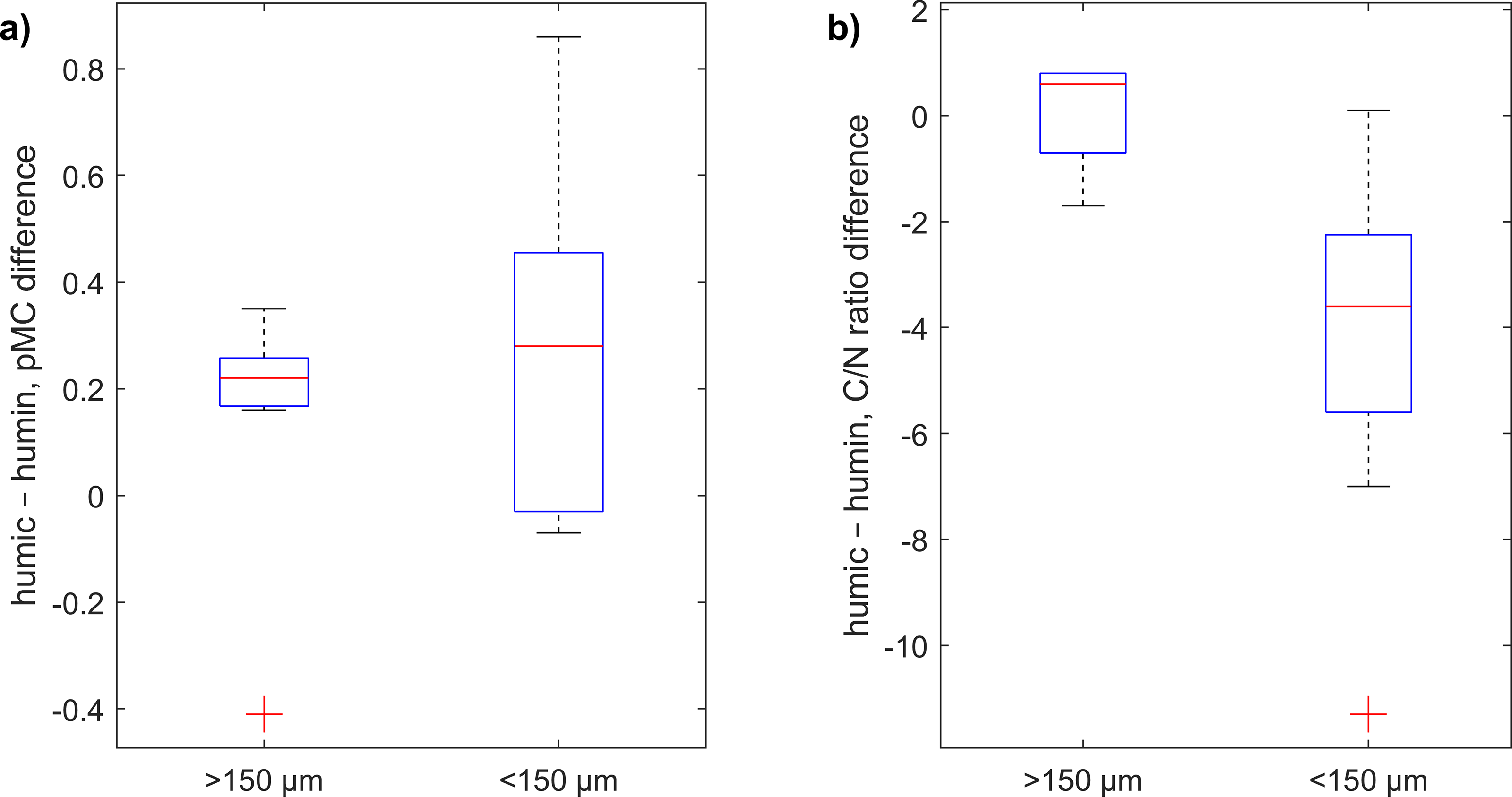
Difference between humic and humin fraction for both >150 µm (n=7), and <150 µm (n=8). a) Radiocarbon content difference expressed in pMC, b) C/N ratio difference. The differences identified as outliers are marked with the plus sign.

Radiocarbon concentration in two analyzed set of layers. a) 6.96–6.99 m; b) 7.11–7.14 m.

Previous palaeoenvironmental reconstructions at Żabieniec site
The findings of Petera-Zganiacz et al. (Reference Petera-Zganiacz, Dzieduszyńska, Milecka, Okupny, Słowiński, Michczyńska, Forysiak and Twardy2022) and Rudna et al. (Reference Rudna, Wojewódka-Przybył, Forysiak, Milecka and Okupny2023) collectively illustrate that the Younger Dryas at the Żabieniec site was characterized by a period of gradual environmental transition rather than abrupt shifts. According to Petera-Zganiacz et al. (Reference Petera-Zganiacz, Dzieduszyńska, Milecka, Okupny, Słowiński, Michczyńska, Forysiak and Twardy2022), the landscape remained relatively stable for during the Younger Dryas without surpassing significant morphogenetic thresholds, while vegetation adapted smoothly through three distinct developmental phases: an initial spread of open tundra and cold steppe communities, a stable middle phase with mild birch increases, and a final transition marked by recovering pine populations. Morphogenetic processes such as soil erosion and mechanical denudation only intensified non-catastrophically toward the end of the Younger Dryas, possibly triggered by wildfires that disturbed the landscape’s stability. Building on this, Rudna et al. (Reference Rudna, Wojewódka-Przybył, Forysiak, Milecka and Okupny2023) utilized Cladocera (water flea) species as sensitive biological indicators to further refine the chronozones of the Late Glacial, providing higher resolution for the specific aquatic responses to cooling and identifying shifts in the lake’s water levels and nutrient status that align with the broader regional climate phases.
Geochemical analysis
Geochemical analysis was performed on the 182 samples at the Institute of Marine and Environmental Sciences University of Szczecin. Among the investigated sedimentary properties of the research core Z-3 were basic lithogeochemical components, such as organic matter (LOI – loss on ignition), biogenic and terrigenous silica (SiO2biog and SiO2ter), biophilic elements (C, N and S), lithophilic elements (Na, K, Mg), total organic carbon (TOC) and carbonate contents (CaCO3). Lithogeochemical analyses of dried samples were performed according to standard procedures, following Borówka (Reference Borówka1990), Müller and Schneider (Reference Müller and Schneider1993), and Pawlik et al. (Reference Pawlik, Okupny, Kroh, Cybul, Stachowicz-Rybka and Sady-Bugajska2022). The organic matter content was determined from the loss on ignition (combustion at 550 °C for 4 hr); the calcium carbonate content (CaCO3) was assayed using the Scheibler apparatus; the terrigenous (SiO2ter) and biogenic (SiO2biog) silica contents were determined following extraction with NaOH. The chemical elements needed for erosion rate calculations: Na, K, Mg and Ca in the deposits were measured as soluble concentrations (using 1.2 N HCl, 15 N HNO3 and H2O2 by Ethos UP microwave mineraliser Milestone company) using atomic absorption spectrometry (AAS iCE 3500, ThermoFisher). The content of total carbon (C), total nitrogen (N) and total sulphur (S) were determined using a Vario Max CNS elemental analyser (model CS530). Moreover, the total organic carbon (TOC) was measured after decalcifying with 1.2 N HCl using an Elemental Analyzer Vario Micro Cube. The described procedure is commonly used for palaeoenvironmental analyses of biogenic accumulation reservoirs in Central European Lowland (e.g. Karasiewicz Reference Karasiewicz2019; Kittel et al. Reference Kittel, Antczak-Orlewska, Apolinarska, Okupny, Makohonienko, Rudna, Rennwanz, Sobczyk, Leszczyk, Płóciennik, Tsvirko, Kotrys, Goslar and Sikora2025; Okupny Reference Okupny2023).
To describe biogenic sediments from the Z-3 core, the classification by Markowski (Reference Markowski1980) was also used, which is based on the content of the main chemical component. The lithological profile of core Z-3 can be summarized as follows: between 6.0 and 8.0 meters, the material consists of coarse detrital gyttja. This transitions to fine detrital gyttja up to 9.44 meters, after which it changes to clay-detrital gyttja. Between 9.98 and 10.80 meters, the core contains clay-mud gyttja with detrital inclusions. This diversification of sediments reflects the changes of conditions and processes occurring in the lake and their catchment.
Chemical pretreatment for the radiocarbon measurements
The Z-3 core was stored in the fridge, then divided into 1 cm thick layers, and selected layers were subjected to macroremains selection. Geochronological analysis was carried out at the Gliwice Radiocarbon Laboratory, Gliwice, Poland. To complement the previously analyzed 11 samples containing macroremains of terrestrial plants from the Younger Dryas, and 1 pollen sample, additional 66 analyses were performed on the samples from depths ranging between 6.60 m and 10.80 m. To assure precision, each layer that was subjected to radiocarbon analysis, was maintained at a 1 cm resolution, where possible. To complement the dataset, additional 11 14C analyses were obtained at 14C lab of the Laboratoire des Sciences du Climat et de l’Environnement, Gif-sur-Yvette, France (Hatté et al. Reference Hatté, Arnold, Dapoigny, Daux, Delibrias, Du Boisgueheneuc, Fontugne, Gauthier, Guillier, Jacob, Jaudon, Kaltnecker, Labeyrie, Noury, Paterne, Pierre, Phouybanhdyt, Poupeau, Tannau, Thil, Tisnérat-Laborde and Valladas2024).
In order to check heterochronousness of the profile, two set of layers were selected for measurements, in which different chemical fractions were isolated. First of the selected interval (6.96–6.99 m) was predicted to fall on one of the steepest segments of the IntCal20 calibration curve (Reimer et al. Reference Reimer, Austin, Bard, Bayliss, Blackwell, Bronk Ramsey, Butzin, Cheng, Edwards, Friedrich, Grootes, Guilderson, Hajdas, Heaton, Hogg, Hughen, Kromer, Manning, Muscheler, Palmer, Pearson, Van Der Plicht, Reimer, Richards, Scott, Southon, Turney, Wacker, Adolphi, Büntgen, Capano, Fahrni, Fogtmann-Schulz, Friedrich, Köhler, Kudsk, Miyake, Olsen, Reinig, Sakamoto, Sookdeo and Talamo2020), reflecting one of the most rapid changes in atmospheric radiocarbon content. This makes the interval well suited for high-resolution dating, as the radiocarbon content changes by approximately 0.7 pMC over about 40 calendar years. Consequently, high-precision measurements from this depth range could be particularly informative (see Figure 3b in Jędrzejowski et al. Reference Jędrzejowski, Hatté, Nadeau, Pawlyta, Rakowski, Sieczkowska-Jacyna and Ustrzycka2025, around 9 540 cal BP, where the “cal BP range” reaches a local minimum). Second set, from 7.11 to 7.14 m, was selected for layers of similar carbon content, but a flatter region of the IntCal20 calibration curve. For these two sets of layers, a more refined analytical procedure was applied. Each sample was divided into five distinct fractions following chemical pretreatment: (1) hand-picked undetermined macroremains, (2) >150 µm humin (acid- and alkali-insoluble fraction), (3) >150 µm humic acid (alkali-soluble, acid-insoluble fraction), (4) <150 µm humin, (5) <150 µm humic acid. A detailed schematic of the chemical pretreatment procedure is provided in Figure 1.
For 16 samples (taken at intervals of about 15 to 20 cm), an Acid–Alkali–Acid (AAA) chemical pretreatment was applied. The samples were neither sieved nor were macroremains picked, as the objective was to preserve as much carbon material as possible for the general model. The procedure involved treatment with 0.5 M HCl for 1 hour at 85 °C, followed by rinsing, then 0.1 M NaOH for 1 hour at 85 °C, rinsing again, and finally 0.5 M HCl for 1 hour at 85 °C, followed by a final rinse and drying of the material. These samples are referred to in this manuscript as “humin without sieving.” Please note, that in the section of the core from approximately 10–11 m depth, the carbon content after chemical pretreatment was very low (from 1.2 to 3.6%).
Whenever possible, macroremains of aquatic and terrestrial plants were also included in the analysis. The samples were prepared chemically in a similar manner to the samples labeled “humin without sieving”, with a difference that the base step was applied at the room temperature.
Combustion, graphitization and radiocarbon measurements
The samples were combusted using an Elementar VarioMicroCube elemental analyzer and graphitized with the AGE-3 automated graphitization system (Wacker et al. Reference Wacker, Němec and Bourquin2010). Each sample was placed in a tin capsule and loaded into a sample carousel. Upon rotation, the capsule was dropped into the combustion chamber, where pure oxygen was introduced to facilitate rapid combustion. The resulting gas was flushed through the elemental analyzer and subsequently transferred to the AGE-3 reactor for further processing.
Following graphitization, the samples, along with reference materials, were measured using the MICADAS spectrometer at the Gliwice Radiocarbon Laboratory (Ustrzycka et al. Reference Ustrzycka, Piotrowska, Kłusek, Pawełczyk, Michczyńska, Michczyński, Kozioł and Jędrzejowski2025). Normalization was done with the Oxalic Acid II (NIST SRM 4990C). Reference materials included IAEA C-5, C-7, C-8, and those from the most recent Glasgow International Radiocarbon Intercomparison (Ustrzycka et al. Reference Ustrzycka, Piotrowska, Kłusek, Pawełczyk, Michczyńska, Michczyński, Kozioł and Jędrzejowski2025 and references therein) and blank wood sample, a fossil wood from the Szczerców opencast at the Bełchatów Lignite Mine (Jędrzejowski et al. Reference Jędrzejowski, Michczyńska, Kłusek, Michczyński, Pawełczyk, Piotrowska, Wyss Heeb and Hajdas2024).
For samples with carbon mass significantly below 0.5 mg, the ECHoMICADAS spectrometer with a Gas Interface System at the Laboratoire des Sciences du Climat et de l’Environnement (LSCE) was utilized. An elemental analyzer allows the samples to be combusted and the resulting CO2 to be purified using the same process as upstream of the AGE-3 system. The CO2 is then directed to a Gas Interface System (GIS), which injects it into the MICADAS ion source (Ruff et al. Reference Ruff, Wacker, Gäggeler, Suter, Synal and Szidat2007; Thil et al. Reference Thil, Tisnérat-Laborde, Hatté, Kader, Noury, Paterne, Phouybanhdyt and Wacker2024).
Radiocarbon results are expressed in pMC that is 100 times F14C, and in 14C conventional age. In this study, calibration was performed with the IntCal20 calibration curve (Reimer et al. Reference Reimer, Austin, Bard, Bayliss, Blackwell, Bronk Ramsey, Butzin, Cheng, Edwards, Friedrich, Grootes, Guilderson, Hajdas, Heaton, Hogg, Hughen, Kromer, Manning, Muscheler, Palmer, Pearson, Van Der Plicht, Reimer, Richards, Scott, Southon, Turney, Wacker, Adolphi, Büntgen, Capano, Fahrni, Fogtmann-Schulz, Friedrich, Köhler, Kudsk, Miyake, Olsen, Reinig, Sakamoto, Sookdeo and Talamo2020).
Age-depth modeling and calibration
Three distinct age-depth models were constructed using different software packages: Bacon, ChronoModel, and OxCal. The objective was to derive robust and universally applicable conclusions that are not overly depend on the specific computational methods or inherent differences between the software packages. In general, OxCal (Bronk Ramsey Reference Bronk Ramsey2009) incorporates prior information about the deposition process via the parameter k. Bacon (Blaauw and Christen Reference Blaauw and Christen2011) requires prior knowledge of sedimentation rates, whereas ChronoModel (Lanos and Philippe Reference Lanos and Philippe2018) does not require such information for its approach.
The OxCal software (Bronk Ramsey Reference Bronk Ramsey2009), which uses Chronological Query Language (CQL), offers several options for modeling depositional processes: D-sequence (where the age gap between points is exact, as in tree rings), V-sequence (where the age gap is approximately known, as in varves), uniform deposition (U-sequence), and P-sequence (which models variable sedimentation through Poisson statistics). The number of depositional events is controlled by the parameter k. Generally, small values of k allow for modeling a variable deposition process, while larger values of k result in more uniform sedimentation rates. Since determining k in advance is often not possible, the common practice is to set a prior distribution for k, typically with a nominal value of k0 and a prior distribution U = log10(k/k0) (Bronk Ramsey and Lee Reference Bronk Ramsey and Lee2013). The goodness of fit for the OxCal age-depth model is expressed by an agreement index (A), with values above 60% considered acceptable. Amodel represents the overall agreement of the model, while Aoverall reflects the agreement indices of individual dates. However, these agreement indices should not be used to select the most probable model, since they do not represent Bayesian factors (Bronk Ramsey Reference Bronk Ramsey1995; Hamilton and Krus Reference Hamilton and Krus2018).
The Bacon software (Blaauw and Christen Reference Blaauw and Christen2011), which is implemented in the R programming language, divides the core into segments and determines accumulation rates using a gamma autoregressive semi-parametric model. This means that the accumulation rate in the current segment depends on that of the previous segment. The priors required by this software are the accumulation rate (in years per centimeter) and the autocorrelation of accumulation rates between segments. Both of these priors are distributions that require specified mean values and shapes. Additionally, the length of the linear segments (and thus their number in the entire core) must be defined.
ChronoModel also employs Bayesian modeling, incorporating the concept of a target event, an event to which the date is applied by the chronometrician, as typically, target events are not directly related to the dated events (Lanos and Philippe Reference Lanos and Philippe2018). The hierarchical structure of this model allows for distinguishing between the date of the event and the date of the material involved in the measurement. It is assumed that the material is contemporaneous with the event, though it may be misallocated (e.g., post-depositional sediment). Outliers are not discarded in ChronoModel, as a high variance automatically reduces their influence on the model. Generally, the robustness of the model results in lower precision of the dates, which, in the context of sedimentation modeling, is acceptable, as it may better reflect the reliability of the chronology.
In the case of OxCal, the P_Sequence model was used, and k0 was set to 1, and the distribution was set to U(−2, 2), so that k varies between 0.01 and 100. In the models, the boundaries were set at the 7.74 m, 8.60 m, 9.20 m,10.09 m.
Results and discussion
AMS results
The main results used for constructing the age–depth models are presented in Table 1. The dataset comprises 41 radiocarbon dates, including 16 from humin without sieving, 21 from terrestrial plant remains, 3 from aquatic plant remains, and 1 from pollen grains. Depending on material availability and carbon content, particularly in the upper section of the core, around 7 m depth, additional measurements were conducted for selected layers of particular interest. For the two specific sets of four consecutive 1-cm layers selected for detailed analysis (6.96–6.99 m and 7.11–7.14 m), an additional 48 radiocarbon measurements were obtained to investigate possible heterochrony within individual sediment layers (Table 2).
Radiocarbon dates from core Z-3 analyzed in this study. Samples with underscored depths were taken from Petera-Zganiacz et al. (Reference Petera-Zganiacz, Dzieduszyńska, Milecka, Okupny, Słowiński, Michczyńska, Forysiak and Twardy2022).

Table 1. Long description
The table presents radiocarbon dating information for sediment samples collected at cumulative depths ranging from 6.60 to 10.81 m. It includes sample fractions, laboratory codes, percent modern carbon (pMC) values, radiocarbon ages, carbon mass, and associated comments. The dated materials comprise humin fractions, terrestrial and aquatic plant remains, pollen, and charcoal. Each sample is identified by its sediment depth and laboratory code, with corresponding pMC measurements and calculated radiocarbon ages. Carbon mass values indicate the quantity of material used for radiocarbon analysis. The comments provide additional information about the nature or identification of the dated material, including plant remains and charcoal. The table allows comparison of radiocarbon ages among different organic fractions and environmental materials recovered from successive sediment depths. The range of sample types provides information for interpreting the chronological sequence and depositional history of the sediment profile. Variations in radiocarbon age with depth and sample material may help distinguish terrestrial and aquatic carbon sources and assess the age structure of the sedimentary sequence.
Comparison of the radiocarbon results for the different fractions obtained from chemical pretreatment, and terrestrial and/or aquatic plants macroremains for selected layers.

Table 2. Long description
The table presents radiocarbon results for different fractions and plant macroremains across selected layers. It has 14 rows and 10 columns. The columns are labeled as Depth in cm, Hand-picked macroremains, >150 μm humic acid, ~150 μm humic acid, <150 μm humic acid, <150 μm humic acid, Terrestrial plants macroremains, and Aquatic plants macroremains. Each row lists values for these columns. Row 1: Depth, 6.96; Hand-picked macroremains, Gda-8434.1.1; >150 μm humic acid, Gda-8434.2; ~150 μm humic acid, Gda-8434.3; <150 μm humic acid, Gda-8434.4; <150 μm humic acid, —; Terrestrial plants macroremains, —; Aquatic plants macroremains, —. Row 2: Depth, 6.97; Hand-picked macroremains, Gda-8435.1.1; >150 μm humic acid, Gda-8435.2; ~150 μm humic acid, Gda-8435.3; <150 μm humic acid, Gda-8435.4; <150 μm humic acid, Gda-8435.5; Terrestrial plants macroremains, Gda-8435.6.1; Aquatic plants macroremains, GifA25641. Row 3: Depth, 6.98; Hand-picked macroremains, Gda-8436.1.1; >150 μm humic acid, Gda-8436.2; ~150 μm humic acid, Gda-8436.3; <150 μm humic acid, Gda-8436.4; <150 μm humic acid, GifA25642; Terrestrial plants macroremains, Gda-8436.6; Aquatic plants macroremains, —. Row 4: Depth, 6.99; Hand-picked macroremains, Gda-8437.1.1; >150 μm humic acid, Gda-8437.2.1; ~150 μm humic acid, Gda-8437.3; <150 μm humic acid, Gda-8437.4; <150 μm humic acid, Gda-8437.5.2; Terrestrial plants macroremains, GifA25644; Aquatic plants macroremains, —. Row 5: Depth, 7.11; Hand-picked macroremains, Gda-8438.1.1; >150 μm humic acid, Gda-8438.2; ~150 μm humic acid, Gda-8438.3.1; <150 μm humic acid, Gda-8438.4; <150 μm humic acid, Gda-8438.5; Terrestrial plants macroremains, Gda-8438.6.1; Aquatic plants macroremains, —. Row 6: Depth, 7.12; Hand-picked macroremains, Gda-8439.1.1; >150 μm humic acid, Gda-8439.2.1; ~150 μm humic acid, Gda-8439.3.1; <150 μm humic acid, Gda-8439.4.1; <150 μm humic acid, Gda-8439.5; Terrestrial plants macroremains, Gda-8439.6.1; Aquatic plants macroremains, —. Row 7: Depth, 7.13; Hand-picked macroremains, Gda-8440.1.1; >150 μm humic acid, Gda-8440.2.1; ~150 μm humic acid, Gda-8440.3.1; <150 μm humic acid, Gda-8440.4.1; <150 μm humic acid, Gda-8440.5; Terrestrial plants macroremains, —; Aquatic plants macroremains, —. Row 8: Depth, 7.14; Hand-picked macroremains, Gda-8441.1.1; >150 μm humic acid, Gda-8441.2.1; ~150 μm humic acid, Gda-8441.3.1; <150 μm humic acid, Gda-8441.4; <150 μm humic acid, Gda-8441.5; Terrestrial plants macroremains, —; Aquatic plants macroremains, —.
Humin fraction vs terrestrial plants across profile
Table 2 presents the 14C contents obtained for the different size and chemical fractions of the sediments. Although statistically compatible, a general tendency emerges toward lower 14C contents (i.e., older apparent ages) in the humin fractions compared to the humic fractions, for both the <150 µm and >150 µm size classes (see Figure 2). This trend can be explained by the chemical treatments applied during the extraction protocol. Following the acid treatment, which removes potential contaminants associated with post-coring microbial activity as well as so-called fulvic acids (organic molecules weakly bound to mineral surfaces), the subsequent alkaline treatment (particularly at elevated temperature) solubilizes the humic acids. These compounds are moderately to strongly bound to mineral surfaces. This process leaves behind the humin fraction, composed of organic molecules that are strongly and persistently bound to mineral surfaces, formed within the lake/peat environment and initially associated with mineral particles prior to their deposition in the sediment. The stronger association of humins with mineral particles likely protects older, pre-depositional organic carbon from degradation and exchange with younger carbon pools, resulting in apparently older radiocarbon ages. These humins are therefore interpreted as organic matter formed within the lake/peat environment or derived from organic matter already associated with mineral particles prior to deposition.
The larger variability observed in the offsets between the pMC values of the humic and humin fractions in the <150 µm size class, compared to the >150 µm fraction (Figure 2a), is most likely related to the proportion of clay particles (<5 µm), which provide the largest specific surface area and therefore constitute the main carriers of mineral-associated organic matter. It is within this fine fraction that the contribution of older carbon, associated with mineral surfaces prior to deposition at the coring site, is expected to be most strongly expressed in the radiocarbon signature. A tendency toward older apparent ages in the fine fraction compared to the coarse fraction is indeed observed (Table 2).
Additional support for this interpretation is provided by the C/N ratios (Figure 2b), which inform on the origin of organic matter in this mixed context of terrestrial inputs (high C/N) and in situ production (low C/N) (Meyers Reference Meyers1994). For both studied levels, in the >150 µm fraction, the humic and humin chemical fractions show no significant difference, with comparable C/N values around 16–18. In contrast, in the fine fraction (<150 µm), a clear distinction appears: the humin fraction displays markedly higher C/N values (up to >25) than the humic acids. This indicates that the organic matter firmly associated with the mineral matrix (resistant to high-temperature ABA treatment) retains a predominantly terrestrial signature, likely inherited from organic matter originally bound to clays before the mineral particles reached the lake/peatland. Conversely, the C/N ratios of the humic acids are closer to those of the <150 µm fraction, although slightly lower on average, suggesting a relatively greater contribution from aquatic matter. In this context of mixed but predominantly distinct organic matter sources, the 1⁴C activity difference between humic acids and humin provides insight into the transit time between the terrestrial and aquatic compartments, defined here as the time elapsed between carbon fixation by photosynthesis and its final incorporation into the sediment. Aquatic organic matter produces within the lake can reach the sediment almost immediately at the timescale considered here. In contrast terrestrial organic matter may undergo several intermediate steps (photosynthesis, plant growth, litter fall, decomposition eventually incorporation into soils, followed by erosion and transport into the lake) before being deposited in the sediment. This sequence of processes introduces a delay between carbon fixation and sediment burial, which refer to her as the transit time. Here, with an offset of ∼0.3 pMC, the transit time is estimated to be less than a century.
Larger moss fragments selected by palaeobotanists (Table 2; Musci) yielded radiocarbon ages consistent with those obtained from the hand-picked unidentified macroremains. However, two samples of terrestrial plants, composed mainly of Musci (GdA-7927.1.1 and GdA-7928.1.1 in Table 1), yielded inconsistent results and were significantly older (see Figure 3). These ages do not correspond well with other fractions taken from the same depth. The reason for this discrepancy remains unresolved so far.
Aquatic plants (Tables 1 and 2) systematically yield younger 14C ages than those obtained from other fractions of the sediment or nearby layers. This pattern falls outside what can reasonably be expected in a palaeoenvironmental context. Post-sampling contamination, potentially involving microbial activity not entirely removed by the chemical pretreatment (as discussed by Wohlfarth et al. Reference Wohlfarth, Skog, Possnert and Holmquist1998), must therefore be considered. Notably, the five samples concerned are very small (masses ranging from 17 to 32 µg), for which chemical pretreatment necessarily represents a compromise between thorough cleaning and preservation of sufficient material to allow measurement. Please note, that reservoir effect for the site is not known, and aquatic samples were calculated with the use of the IntCal20 (Reimer et al. Reference Reimer, Austin, Bard, Bayliss, Blackwell, Bronk Ramsey, Butzin, Cheng, Edwards, Friedrich, Grootes, Guilderson, Hajdas, Heaton, Hogg, Hughen, Kromer, Manning, Muscheler, Palmer, Pearson, Van Der Plicht, Reimer, Richards, Scott, Southon, Turney, Wacker, Adolphi, Büntgen, Capano, Fahrni, Fogtmann-Schulz, Friedrich, Köhler, Kudsk, Miyake, Olsen, Reinig, Sakamoto, Sookdeo and Talamo2020).
Outliers
The radiocarbon results for samples from depths of 6.83 m, 8.44 m and 9.98 m have been identified as potential outliers. The 8.44 m sample consisted of pollen grains, which may reflect environmental conditions differing from those represented by the surrounding sediment, and different age, which is consistent in the literature (e.g. Schiller et al. Reference Schiller, Whitlock, Elder, Iverson and Abbott2021; Zimmerman et al. Reference Zimmerman, Brown, Hassel and Heck2019). The 6.83, and 9.98 m samples, representing the humin without sieving fraction, were addressed by measuring terrestrial and aquatic macoremains from those or nearby depths. However, it was found that both types of macroremains yielded ages significantly younger than expected based on the established stratigraphic chronology, which may be linked to the sampling, as those depths represents where the core parts were divided into ∼1 m pieces.
Age-depth models
The three age-depth models generally show good agreement, with a few exceptions (see Figure 4). In the upper section of the core, between approximately 6.5 and 7.2 meters, the radiocarbon dates after calibration are rather problematic, as discussed earlier. As a result, the models in Bacon and OxCal indicate a phase of rapid accumulation, whereas Chronomodel suggests a different chronology, assuming slower accumulation during this interval. Below this depth, the models follow broadly similar trends, though differences emerge in how the dates are treated, leading to slight misalignment, and in the degree of smoothing applied to the modeled results. Specifically, OxCal connects the data points with straight lines, while Chronomodel applies stronger smoothing. For instance, compare the curves (“elbows”) around 7.7 m and 8.6 m, as in these sections the most significant distinctions between the models occur. Overall, however, the results below 7.0 m are consistent within the 95.4% confidence interval.
Age-depth models comparison. For the construction of the model, 34 dates from different layers were used, of which four were identified as outliers.

Lithogeochemical evidence
The profile Z-3 was subdivided into lithostratigraphical units in accordance with lithological properties observed during fieldwork, and the results of the laboratory analyses. In general, the depth interval between 10.94 and 10.18 m consists of a mineral layer, whereas the upper part of the core (depth: 10.10–7.30 m) contains more organic components. Sediments deposited at the depth of 10.18–10.10 m comprise the transition zone between mineral and organic. The chemical composition of the clay gyttja (depth below 10.18 m) showed that the dominant component of the sediment is mineral matter, as it oscillates between 90 and 97%. The second most abundant component is organic matter (mean 4.7%) and total organic carbon (mean 1.7%), with the complete lack of SiO2biog and CaCO3. Moreover, the erosion ratio calculated as (Na+K+Mg)/Ca, showed a mean value of 0.85 in the mineral deposits. In the transition layer, total organic carbon increases from 3.9 to 8.4%. The part of the Z-3 core above 10.10 m represents clay-detritus gyttja with dynamic changes in the content of lithophilic elements, such as Na, K and Mg. The content of organic components, such as organic matter and total organic carbon increased to about 40% and about 20% respectively (Figure 5a–b). The initiation of more organic sediments is reflected by the variable erosion ratio (Figure 5c).
a) Organic matter content; b) Total organic carbon (TOC) content; c) Erosion Index; d) Sedimentation rate for the organic matter; e) Sedimentation rate for the inorganic matter. Sedimentation rates are based on an OxCal model (blue dots), ChronoModel (green squares), and Bacon model (black stars). The thinner lines represent original data without smoothing. The points mark the actual sample positions (after modelling and smoothing). Greenland Stadials (GS) and Greenland Interstadials (GI) according to INTIMATE event stratigraphy of Rasmussen et al. (Reference Rasmussen, Bigler, Blockley, Blunier, Buchardt, Clausen, Cvijanovic, Dahl-Jensen, Johnsen, Fischer, Gkinis, Guillevic, Hoek, Lowe, Pedro, Popp, Seierstad, Steffensen, Svensson, Vallelonga, Vinther, Walker, Wheatley and Winstrup2014), while chronozones of the Late Glacial for the area follow Petera-Zganiacz et al. (Reference Petera-Zganiacz, Dzieduszyńska, Milecka, Okupny, Słowiński, Michczyńska, Forysiak and Twardy2022), and Rudna et al. (Reference Rudna, Wojewódka-Przybył, Forysiak, Milecka and Okupny2023). Abbreviation: O.D. – Older Dryas.

Figure 5. Long description
Panel A: A line graph shows the organic matter content over time. The x-axis represents age in calBP (calibrated years before present), ranging from 18,000 to 10,000 years. The y-axis represents the core depth in meters. The graph shows fluctuations in organic matter content over time. Panel B: A line graph displays the total organic carbon (TOC) content over time. The x-axis represents age in calBP, and the y-axis represents the TOC percentage. The graph shows variations in TOC content over the same time period. Panel C: A line graph illustrates the erosion index over time. The x-axis represents age in calBP, and the y-axis represents the erosion index. The graph shows peaks and troughs in the erosion index. Panel D: A line graph depicts the sedimentation rate for organic matter over time. The x-axis represents age in calBP, and the y-axis represents the sedimentation rate in centimeters per year. The graph includes data points from Bacon, OxCal, and ChronoModel models, showing different sedimentation rates. Panel E: A line graph shows the sedimentation rate for inorganic matter over time. The x-axis represents age in calBP, and the y-axis represents the sedimentation rate in centimeters per year. The graph also includes data points from Bacon, OxCal, and ChronoModel models, showing different sedimentation rates. The graphs are overlaid with different models and show trends in sedimentation rates for both organic and inorganic matter.
Sedimentation rate
Based on the age-depth models constructed using Bacon, ChronoModel, and OxCal, sedimentation rates were calculated at a 1 cm resolution. To reduce numerical noise and small peaks caused by calculations (e.g. resulting from boundaries), the results were smoothed using a moving average. It is important to note that sediment compaction was not taken into account, so the calculated sedimentation rates should be considered approximate.
Based on the loss on ignition, the organic content was assessed, and as mentioned earlier, shows considerable variability (see Figure 5a). The data are available from 7.3 m to 10.8 m core depth, with a 2 cm resolution. For simplicity, geochemical parameters are plotted as a function of age, based on the OxCal model, while original depth axis is also shown with the organic matter figure (Figure 5a). The calculated sedimentation rates were subsequently multiplied by the organic and inorganic content, in order to analyze different sources of material.
The Greenland Stadials and Greenland Interstadials are shown according to the INTIMATE event stratigraphy (Rasmussen et al. Reference Rasmussen, Bigler, Blockley, Blunier, Buchardt, Clausen, Cvijanovic, Dahl-Jensen, Johnsen, Fischer, Gkinis, Guillevic, Hoek, Lowe, Pedro, Popp, Seierstad, Steffensen, Svensson, Vallelonga, Vinther, Walker, Wheatley and Winstrup2014), while the chronozones of the Late Glacial for the area are based on Petera-Zganiacz et al. (Reference Petera-Zganiacz, Dzieduszyńska, Milecka, Okupny, Słowiński, Michczyńska, Forysiak and Twardy2022), and Rudna et al. (Reference Rudna, Wojewódka-Przybył, Forysiak, Milecka and Okupny2023), and the detailed multiproxy analysis presented therein.
In the case of the organic matter, sedimentation was extremely low from around 18 cal kBP to 15.5 cal kBP (Figure 5d). Then, sedimentation increased up to around 14 cal kBP, which is visible also in other parameters: TOC (Figure 5b), and the erosion index (Figure 5c). Then within the Older Dryas (roughly around GI-1d) sedimentation reached a local maximum. After that, the organic sedimentation rate reached a local minimum, which may be associated with the Older Dryas/Allerød transition, and continued with a low sedimentation rate. After about the middle of the Allerød, sedimentation began to increase, reaching another local maximum (roughly coinciding with GI-1b). Then, during the Younger Dryas, sedimentation was relatively stable from around 11.8 cal kBP, which coincides with the end of GS-1. Near the end of the Younger Dryas at this site, and at the time when the INTIMATE chronology changes from GS-1 to the Holocene, a huge injection of organic matter occurred. At the very end of the Younger Dryas at this site, another large injection of organic matter is observed, coinciding with the 11.4 ka b2k event from the INTIMATE chronology. Based on the timeframe and chronozones described by Petera-Zganiacz et al. (Reference Petera-Zganiacz, Dzieduszyńska, Milecka, Okupny, Słowiński, Michczyńska, Forysiak and Twardy2022), the Younger Dryas/Holocene transition seems to occur later compared to the INTIMATE chronology; therefore, the archive recorded both global and local conditions.
Changes in the inorganic matter show a similar pattern (Figure 5e). Until about 15.5 cal kBP, the sediment was dominated by inorganic matter, resulting in a much higher sedimentation rate. The organic component began to dominate after the onset of the Holocene.
Conclusions
The development of a reliable, high-resolution age-depth model is a multi-stage process that is highly sensitive to the quality and selection of dated material. Material heterogeneity and heterochrony represent key challenges, as the Żabieniec core posed particular difficulties in establishing a coherent chronology. A robust radiocarbon framework for the Żabieniec sediment sequence was established using three independent age–depth modeling approaches (OxCal, Bacon, and ChronoModel).
The comparison of dated materials demonstrates that:
-
The “humin without sieving” fraction, used for the general model when preserved organic matter was scarce or ultrafine, proved that the use of such a fraction may be beneficial in order to establish a chronology for the site. The few outliers may indicate post-depositional disturbance, or contamination during sampling, when modern material can be pushed down with the corer.
-
Terrestrial macroremains are reliable dating material, and isolating well-defined terrestrial plant macrofossils is strongly recommended. Although in this study, some samples yielded anomalous results. Aquatic plants, which often introduce a reservoir effect, in this case yielded ages significantly younger than expected based on the stratigraphic context, which may require further investigations. In all cases the amount of macroremains is low, therefore they may not be a reliable representation of the dated layers.
-
Chemically isolated fractions (hand-picked macroremains, humin, and humic acid) fractions were generally consistent across the tested layers, although minor variations in radiocarbon content indicate subtle mixing or reworking within the sediment.
-
The offset of ∼0.3 pMC between the terrestrial and aquatic compartments, suggests that the transit time is less than a century.
Organic matter sedimentation was very low until from ∼18 to ∼15.5 cal kBP, increased with peak during the Older Dryas and then peak mid-Allerød, and remained relatively stable through most of the Younger Dryas. At the end of the Younger Dryas, sedimentation reached another maximum. All age–depth models indicate changes in the sedimentation rates of both the organic and mineral fractions of the deposits, in excellent agreement with the boundaries defined by the INTIMATE stratigraphy. In particular, onset of GI-1d, onset of GI-1b, the GI-1/GS-1 transition, the GS-1/Holocene transition, and the 11.4 ka event are marked by increased sedimentation rates (see maxima in Figure 5d–e). This suggests that sedimentation rates responded to climate changes synchronously (within the limits of the age–depth model uncertainty) with the changes recorded in the Greenland ice cores.
The resulting chronology and sedimentation rates provide a solid temporal framework for interpreting the main palaeoenvironmental changes recorded at the Żabieniec site within the broader context of the Late Glacial and Holocene global and regional climate variability. These findings emphasize the importance of combining multiple material types, chemical pretreatments, and modeling approaches to achieve reliable, high-resolution chronologies in complex sedimentary archives.
Acknowledgments
We sincerely thank Joanna Petera-Zganiacz for providing Z-3 core for this research project. We sincerely thank Alicja Ustrzycka and the staff at the Gliwice Radiocarbon Laboratory for their assistance throughout the course of conducting the radiocarbon measurements.
Geochemical analysis was co-financed by the Ministry of Science under the “Regional Excellence Initiative” Program for 2024-2027 (project No. RID/SP/0045/2024/01).