2.1 Observation function

The observation function of the carrier phase is written as

(1)\begin{equation}\lambda \varphi _i^j = \rho _i^j + c\delta t^j-c\delta t_i + \lambda N + \delta d_{{\rm eph}}-\delta d_{{\rm iono}} + \delta d_{{\rm trop}} + \eta \end{equation}

where subscript i denotes the receiver number, superscript j denotes the satellite number, $\lambda$ is the wavelength, $\varphi _i^{\; j}$ represents the measured carrier phase expressed in cycle, $\rho _i^{\; j}$ stands for the geometric range from satellite to receiver, c is the speed of light, $\delta t^{\; j}$ and $\delta t_i$ denote the satellite and receiver clock bias, N represents the integer ambiguity. $\delta d_{{\rm eph}}$, $\delta d_{{\rm iono}}$ and $\delta d_{{\rm trop}}$ are ephemeris error, troposphere delay and ionosphere delay, respectively, the last term $\eta$ is regarded as measurement noise. Even if there is no cycle slip, it is difficult to determine the integer ambiguity. However, the ambiguity can be regarded as constant without cycle slip, so we can eliminate it through single difference between successive epochs. And the observation function of TDCP is expressed as

(2)\begin{equation}\lambda \Delta \varphi {\rm} = \lambda \cdot [\varphi _i^j (t_k)-\varphi _i^j (t_{k-1})] = \Delta \rho + c\Delta \delta t^j+c\Delta \delta t_i + \Delta \delta d_{{\rm eph}} + \Delta \delta d_{{\rm trop}}-\Delta \delta d_{{\rm iono}} + \Delta \eta \end{equation}

where $t_k$ and $t_{k\unicode{x2013} 1}$ are two GPS epochs, ${\rm \Delta }$ represents the difference operation. For instance, ${\rm \Delta }\rho {\rm} = \rho _i^{\; j} (t_k)\unicode{x2013} \rho _i^{\; j} (t_{k\unicode{x2013} 1})$ is the change in geometric distance between two epochs, and other terms in Equation (2) are defined accordingly. The TDCP observations can mitigate troposphere delay and ionosphere delay due to their close temporal and spatial correlation during short time intervals (Ding and Wang, Reference Ding and Wang2011). Moreover, the same satellite ephemeris will be used between adjacent epochs avoiding inconsistent results (Freda et al., Reference Freda, Angrisano, Gaglione and Troisi2015). As a result, we can ignore the satellite ephemeris errors. In addition, the Saastamoinen model and Klobuchar model are used to calculated troposphere delay and ionosphere delay for improving the estimation accuracy. Therefore, the TDCP measurement model can be rewritten as Equations (3)–(6), and the unknown parameter (position increment) ${\rm \Delta }\boldsymbol{r}_i$ is calculated by Equation (3).

(3)\begin{gather}\lambda \Delta \tilde{\varphi } = \lambda \Delta \varphi -\Delta D + \Delta g = {-}[\boldsymbol{e}(t_k)\cdot \Delta \boldsymbol{r}_i] + c\Delta \delta t_i + \Delta \eta \end{gather}

(4)\begin{gather}\Delta D = [\boldsymbol{e}(t_k)\cdot \boldsymbol{r}^j(t_k)]-[\boldsymbol{e}(t_{k-1})\cdot \boldsymbol{r}^j(t_{k-1})]\end{gather}

(5)\begin{gather}\Delta g = [\boldsymbol{e}(t_k)\cdot \boldsymbol{r}_i(t_{k-1})]-[\boldsymbol{e}(t_{k-1})\cdot \boldsymbol{r}_i(t_{k-1})]\end{gather}

(6)\begin{gather}\boldsymbol{e}(t_k) = \displaystyle{{\boldsymbol{r}^j(t_k)-\boldsymbol{r}_i(t_k)} \over {||{\boldsymbol{r}^j(t_k)-\boldsymbol{r}_i(t_k)} ||}}\boldsymbol{, e}(t_{k-1}) = \displaystyle{{\boldsymbol{r}^j(t_{k-1})-\boldsymbol{r}_i(t_{k-1})} \over {||{\boldsymbol{r}^j(t_{k-1})-\boldsymbol{r}_i(t_{k-1})} ||}}\end{gather}

where $\boldsymbol{r}^{\; j}$ and $\boldsymbol{r}_i$ are the satellite position vector and receiver position vector, and a⋅b is the inner product of vectors a and b. The terms ${\rm \Delta }g$ and ${\rm \Delta }D$ are caused by relative motion of receiver and satellite from signal transmission moment to signal receive moment, respectively. Based on Equation (3), ${\rm \Delta }\boldsymbol{r}_i$ and ${\rm \Delta }t_i$ can be estimated by KF. Hence, the final average velocity vector is

(7)\begin{equation}\boldsymbol{V} = \displaystyle{{\Delta \boldsymbol{r}_i} \over {t_k-t_{k-1}}}\end{equation}

It is worth noting that the displacement increment estimated by Equation (3) is not an average value, but precise baseline measurement between two consecutive epochs (Ding and Wang, Reference Ding and Wang2011). However, using TDCP to estimate the velocity has a major limitation – the displacement increment divided by time is the average velocity.

2.2 Parameter estimation method

2.2.1 Kalman filter

We can utilise KF to estimate the parameter in Equation (3). The system state model of KF is described as follows.

(8)\begin{gather}\boldsymbol{X}_k = \boldsymbol{F}_{k/k-1}\boldsymbol{X}_{k-1} + \boldsymbol{w}_k\end{gather}

(9)\begin{gather}\boldsymbol{Z}_k = \boldsymbol{H}_k\boldsymbol{X}_k + \boldsymbol{v}_k\end{gather}

where $\boldsymbol{F}_{k/k\unicode{x2013} 1}$ denotes the state transition matrix; $\boldsymbol{w}_k$ is system noise and $\boldsymbol{w}_k{\rm \sim (}{\bf 0}{\rm ,\; }\boldsymbol{Q}_k)$, $\boldsymbol{H}_k$ is the linearised coefficient matrix, $\boldsymbol{v}_k$ is measurement noise and $\boldsymbol{v}_k{\rm \sim }({{\bf 0}{\rm ,\; }\boldsymbol{R}_k} ) .$ Moreover, ${\rm E}[{\boldsymbol{w}_k,\boldsymbol{v}_j} ]{\rm} = 0$. $\boldsymbol{Q}_k$ and $\boldsymbol{R}_k$ are the state and measurement noise covariance, respectively. KF is divided into state update and measurement update. Equations (10) and (11) constitute the state update, while Equations (12)–(14) comprise the measurement update in KF.

(10)\begin{gather}\boldsymbol{X}_{k/k-1} = \boldsymbol{F}_{k/k-1}\boldsymbol{X}_{k-1}\end{gather}

(11)\begin{gather}\boldsymbol{P}_{k/k-1} = \boldsymbol{F}_{k/k-1}\boldsymbol{P}_{k-1}\boldsymbol{F}_{k/k-1}^T + \boldsymbol{Q}_k\end{gather}

where $\boldsymbol{X}_{k/k\unicode{x2013} 1}$ and $\boldsymbol{P}_{k/k\unicode{x2013} 1}$ are the predicted state vector and its covariance.

(12)\begin{gather}\boldsymbol{K}_k = \boldsymbol{P}_{k/k-1}\boldsymbol{H}_k^T (\boldsymbol{H}_k\boldsymbol{P}_{k/k-1}\boldsymbol{H}_k^T + \boldsymbol{R}_k)^{{-}1}\end{gather}

(13)\begin{gather}\boldsymbol{X}_k = \boldsymbol{X}_{k/k-1} + \boldsymbol{K}_k(\boldsymbol{Z}_k-\boldsymbol{H}_k\boldsymbol{X}_{k/k-1})\end{gather}

(14)\begin{gather}\boldsymbol{P}_k = (\boldsymbol{I}-\boldsymbol{K}_k\boldsymbol{H}_k)\boldsymbol{P}_{k/k-1}\end{gather}

where $\boldsymbol{K}_k$ is the gain matrix of KF, $\boldsymbol{X}_k$ and $\boldsymbol{P}_k$ are the updated state vector and its covariance.

Sometimes, the classic KF cannot estimate the parameter correctly under complex observation condition. Besides, this paper adopts the assumption of constant speed model in the state update, and TDCP estimates the average velocity. Hence, ARKF is needed to improve the accuracy of parameter estimation.

2.2.2 ARKF

ARKF is divided into two parts: adaptive KF (AKF) and robust KF (RKF). Due to the constraints of average speed estimated by TDCP, there is a deviation between the predicted state and actual state. To balance the contribution of predicted state and observation, the state noise covariance must be adjusted, that is, AKF. As a result, covariance matching is applied based on the innovation method to adaptively caculate $\skew{3}\hat{\boldsymbol{Q}}_k$ (Mohamed and Schwarz, Reference Mohamed and Schwarz1999; Meng et al., Reference Meng, Gao, Zhong, Hu and Subic2016).

(15)\begin{gather}\skew{3}\hat{\boldsymbol{Q}}_k = \displaystyle{1 \over m}\sum\limits_{j = k-m+1}^{k} {{\tilde{\boldsymbol{V}}}_j\tilde{\boldsymbol{V}}_j^T } + \boldsymbol{P}_k-\boldsymbol{F}_{k/k-1}\boldsymbol{P}_{k-1}\boldsymbol{F}_{k/k-1}^T \end{gather}

(16)\begin{gather}\tilde{\boldsymbol{V}}_j = \boldsymbol{Z}_j-\boldsymbol{H}_j\boldsymbol{X}_{j/j-1}\end{gather}

where $\tilde{V}_j$ denotes the innovation matrix at epoch j, and m is the size of the sliding window. Hence, the predicted state covariance in AKF can be expressed as follows.

(17)\begin{equation}\boldsymbol{P}_{k/k-1} = \boldsymbol{F}_{k/k-1}\boldsymbol{P}_{k-1}\boldsymbol{F}_{k/k-1}^T + \hat{\boldsymbol{Q}}_k\end{equation}

The purpose of RKF is to reduce the weight of observation with gross errors, and reduce the influence of these observations on parameter estimation. A two-stage RKF is adopted, and the constant value c is 1⋅0.

(18)\begin{equation}\lambda _{ii} = \left\{\begin{matrix}1 & {|{{\bar{\boldsymbol{V}}}_i} |\le c}\\ {\displaystyle{{|{{\bar{\boldsymbol{V}}}_i} |} \over c}} & {|{{\bar{\boldsymbol{V}}}_i} |> c} \end{matrix} \right.\end{equation}

where $\bar{\boldsymbol{V}}_i = \tilde{\boldsymbol{V}}_i/\sigma _{{\tilde{\boldsymbol{V}}}_i}$ at epoch k, $\sigma _{{\tilde{\boldsymbol{V}}}_i}$ is the root mean square error of $\tilde{\boldsymbol{V}}_i$, subscript i represents the satellite number, $\lambda _{ii}$ denotes diagonal elements of ${\bf \lambda }$. The gain matrix in RKF is expressed as follows.

(19)\begin{equation}\boldsymbol{K}_k = \boldsymbol{P}_{k/k-1}\boldsymbol{H}_k^T (\boldsymbol{H}_k\boldsymbol{P}_{k/k-1}\boldsymbol{H}_k^T + \boldsymbol{\lambda }\boldsymbol{R}_k)^{{-}1}\end{equation}

3.1 Doppler velocimetry

Doppler observation is the frequency difference between the receiving signal and transmitting signal due to the relative motion between receiver and satellite. The Doppler observation can be used for instantaneous measurement of velocity. Assuming that the transmission frequency of the satellite signal is f, the Doppler effect occurs due to the relative motion between satellite and receiver, resulting in a deviation between the signal receiving frequency f_r and original frequency f, which is the Doppler frequency shift, also known as the Doppler observation. The Doppler frequency shift reflects the change rate of pseudorange, and the pseudorange observation equation is

(20)\begin{equation}\rho _i^j = \boldsymbol{e}_i^j \cdot (\boldsymbol{x}^j-\boldsymbol{x}_i) + c\delta t_i-c\delta t^j + \delta d_{{\rm iono}} + \delta d_{{\rm trop}} + \varepsilon \end{equation}

where $\boldsymbol{e}_i^{\; j}$ represents direction cosine matrix, $\boldsymbol{x}^j$ and $\boldsymbol{x}_i$ represent the position of jth satellite and ith receiver in Earth centred Earth fixed (ECEF), $\varepsilon$ is the observation error. The relationship of Doppler observation and change rate of the pseudorange $\dot{\rho }_i^j$ can be written as

(21)\begin{equation}{-}\lambda D_i^j = \dot{\rho }_i^j = \boldsymbol{e}_i^j \cdot (\boldsymbol{v}^j-\boldsymbol{v}_i) + c\delta \dot{t}_i + \dot{\varepsilon }\end{equation}

where $D_i^{\; j}$ is the Doppler measurement, unit of which is Hz, $v^{\; j}$ and $v_i$ denote the speed of jth satellite and ith receiver, respectively, $\delta \dot{t}_i$ is the change rate of receiver clock, $\dot{\varepsilon }$ is referred to as residual error. In addition, Doppler velocimetry needs to calculate the satellite velocity based on satellite ephemeris, which hinders the application of real-time positioning.

3.2 Doppler enhanced TDCP model

When the receiver is in a dynamic or complex environment, the Doppler observation has a higher accuracy and is more reliable, therefore it is necessary to integrate TDCP velocimetry and Doppler velocimetry. The Doppler shift can be approximated from carrier phase measurements using first order central difference (Cannon et al., Reference Cannon, Lachapelle, Szarmes, Hebert, Keith and Jokerst1997; Ryan et al., Reference Ryan, Lachapelle and Cannon1997). If the interval between adjacent epochs is 1 s, then we can obtain Equation (22).

(22)\begin{equation}D_i^j (t_k) = {-}\displaystyle{{\varphi (t_{k + 1})-\varphi (t_{k-1})} \over 2}\approx{-}[\varphi (t_k)-\varphi (t_{k-1})]\end{equation}

To reduce the approximate error of derived Doppler, the integration method was adopted to deduce the relationship.

(23)\begin{equation}\Delta \varphi (t_k) = \varphi (t_k)-\varphi (t_{k-1}) = \int_{t_{k-1}}^{t_k} {-D_i^j (t)dt} \approx{-}\displaystyle{{D_i^j (t_k) + D_i^j (t_{k-1})} \over 2} \times \Delta t = {-}\displaystyle{{D_i^j (t_k) + D_i^j (t_{k-1})} \over 2}\end{equation}

Substitute Equation (23) into Equation (3), and the Doppler enhanced TDCP approach is expressed as

(24)\begin{equation}{-}\lambda \displaystyle{{D_i^j (t_k) + D_i^j (t_{k-1})} \over 2}-\Delta D + \Delta g = {-}\boldsymbol{e}(t_k)\cdot \Delta \boldsymbol{r}_i + c\delta t_i + \varepsilon \end{equation}

The modified TDCP method inherits the advantages of Doppler method and TDCP method, including: (1) improved velocimetry based on Doppler observations, which makes the observations more reliable when the carrier is in a dynamic and complex observation environment; (2) there is no need to calculate the satellite speed in advance, which is beneficial to the implementation of real-time velocity measurement.

3.3 TARKF

The AKF in Section 2.2 takes into account the error between the average speed and instantaneous speed, and ignores the effect caused by constant speed state update model. Therefore, on the basis of the aforementioned AKF, this paper proposes a TAKF to fuse historical state information and measurement information. In ARKF, predicted state covariance can be expressed as

(25)\begin{equation}\bar{\boldsymbol{P}}_{k/k-1} = \beta \boldsymbol{P}_{k/k-1}\end{equation}

The main task is to estimate the parameter $\beta$.

The variables, three variables of delta position and a variable of change of receiver clock, can be used to fit the function to time in Equation (26).

(26)\begin{align} \begin{bmatrix} \Delta r_{i_x} \\ {\Delta r_{i_y}} \\ {\Delta r_{i_z}} \\ {\Delta \delta t_i} \end{bmatrix} = \boldsymbol{A}t^2 + \boldsymbol{B}t + \boldsymbol{C}\end{align}

where ${\rm \Delta }r_{i_x}$, ${\rm \Delta }r_{i_y}$, ${\rm \Delta }r_{i_z}$ denote the receiver's displacements of coordinate axes in ECEF, A, B, C are unknown four-dimensional coefficient matrices, which can be estimated by three epochs before the current epoch, and t represents the relative time interval. There are two main reasons why the current state can be predicted based on the historical state. The existence of inertia makes the change of motion state of on-board receiver continuous. For example, a normal driving car will not immediately decelerate to a speed and displacement become zero. Moreover, in the design of roads, due to the limitations of natural conditions and features, the highway is composed of straight lines and curves in both plane and longitudinal planes, and most of the curves can be fitted to polynomials. The layout of the road restricts the driving of vehicles. So, in the movement of vehicle receiver, the route can be abstracted as a quadratic function related to time.

Yang proposed an AKF based on the prior state and posterior state of KF (Yang, Reference Yang2001), but this method requires the construction of a state discrepancy statistics test after the measurement update. Instead, it is possible to predict two sets of parameters through state update and binomial fitting before measurement update to construct the state discrepancy statistic as follows.

(27)\begin{gather}\Delta \boldsymbol{X}_k\boldsymbol{= }\displaystyle{{||{{\hat{\boldsymbol{x}}}_k\unicode{x2013} {\bar{\boldsymbol{x}}}_k} ||} \over \sigma }\sim N(0,1)\end{gather}

(28)\begin{gather}||{{\hat{\boldsymbol{x}}}_k-{\bar{\boldsymbol{x}}}_k} || = (dx_{k_1}^2 + dx_{k_2}^2 + dx_{k_3}^2 + dx_{k_4}^2 )^{1/2} = (d\boldsymbol{x}^Td\boldsymbol{x})^{1/2}\end{gather}

(29)\begin{gather}dx_i = \hat{x}_{k_i}-\bar{x}_{k_i},i = 1,2,3,4\end{gather}

(30)\begin{gather}\sigma ^2 = \displaystyle{{{(d\boldsymbol{x}_k)}^T{\bar{\boldsymbol{P}}}_{k,k-1}(d\boldsymbol{x}_k)} \over {m-n}}\end{gather}

where $\hat{x}$ and $\bar{x}$ denote the prior state after state update and predicted state obtained by binomial fitting at epoch k, respectively, m and n represent the number of measurements and estimated states.

If both the prior state and binomial fitted state are correct, the statistics of state discrepancy should conform to the normal distribution with a mean of zero. Once the discrepancy statistics are greater than the limit, it can be considered that there is a problem with the state update. Its limit is defined as

(31)\begin{equation}P\{{\Delta \boldsymbol{X}_k > \varPhi (\alpha )} \} = 1-\alpha \end{equation}

where ${\rm \alpha }$ denotes the probability that $\Delta \boldsymbol{X}_k$ is greater than $\varPhi (\alpha )$, $P\{{\cdot} \}$ represents the probability of a random event occurring. In the process of KF, it is assumed that the state update is correct, and the incorrect update is a small probability event. Equation (31) can be regarded as judging whether the state update is a small probability event, that is, $\Delta \boldsymbol{X}_k$ greater than $\varPhi (\alpha )$ should be a small probability event. This paper assumes that $\alpha$ corresponds to the probability of 90%, so the error probability of error update is less than 10%, where $\varPhi (\alpha )$ corresponds to 1⋅28.

According to Equation (31) we can obtain the function of $\beta$ in Equation (32)

(32)\begin{equation}f(\beta ) = \displaystyle{{\sqrt {d\boldsymbol{x}^Td\boldsymbol{x}} } \over {\sqrt {((d\boldsymbol{x}^T{\bar{\boldsymbol{P}}}_{k/k-1}d\boldsymbol{x})\boldsymbol{/}(m-n))} }}-\varPhi (\alpha ) = 0\end{equation}

In view of the fact that Equation (32) is a nonlinear expression about $\beta$, it can be solved by the Newton iteration (Chang, Reference Chang2014)

(33)\begin{gather}\beta _{i + 1} = \beta _i-\displaystyle{{f(\beta _i)} \over {{f}^{\prime}(\beta _i)}}\end{gather}

(34)\begin{gather}\beta (i + 1) = \beta (i) + 2 \times \displaystyle{{\sqrt {d\boldsymbol{x}^Td\boldsymbol{x}} ((d\boldsymbol{x}^T{\bar{\boldsymbol{P}}}_{k/k-1}d\boldsymbol{x})/(m-n))-\varPhi (\alpha ){({(d\boldsymbol{x}^T{\bar{\boldsymbol{P}}}_{k/k-1}d\boldsymbol{x})/(m-n)} )}^{3/2}} \over {\sqrt {d\boldsymbol{x}^Td\boldsymbol{x}} ((d\boldsymbol{x}^T\boldsymbol{P}_{k/k-1}d\boldsymbol{x})/(m-n))}}\end{gather}

After obtaining β from Equations (33) and (34), we can construct the TARKF. The state update process is as expressed in Equations (35) and (36), and the measurement update process is as written in Equations (37)–(39).

(35)\begin{gather}\boldsymbol{X}_{k/k-1} = \boldsymbol{F}_{k/k-1}\boldsymbol{X}_{k-1}\end{gather}

(36)\begin{gather}\boldsymbol{P}_{k/k-1} = \boldsymbol{F}_{k/k-1}\boldsymbol{P}_{k-1}\boldsymbol{F}_{k/k-1}^T + \hat{\boldsymbol{Q}}_k\end{gather}

(37)\begin{gather}\boldsymbol{K}_k = \beta \boldsymbol{P}_{k/k-1}\boldsymbol{H}_k^T (\boldsymbol{H}_k\beta \boldsymbol{P}_{k/k-1}\boldsymbol{H}_k^T + \boldsymbol{\lambda }\boldsymbol{R}_k)^{{-}1}\end{gather}

(38)\begin{gather}\boldsymbol{X}_k = \boldsymbol{X}_{k/k-1} + \boldsymbol{K}_k(\boldsymbol{Z}_k-\boldsymbol{H}_k\boldsymbol{X}_{k/k-1})\end{gather}

(39)\begin{gather}\boldsymbol{P}_k = (\boldsymbol{I}-\boldsymbol{K}_k\boldsymbol{H}_k)\beta \boldsymbol{P}_{k/k-1}\end{gather}

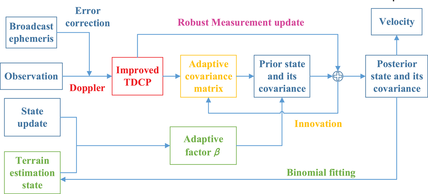
It can be seen from the above analysis that this method mainly modifies the prior state covariance matrix based on the state discrepancy statistic. When the statistic is greater than the limit, the β will be increased, which will increase the value of gain matrix K_k in the measurement update to balance the weight of predicted state and measurement. The process of Doppler enhanced TDCP based on TARKF is shown in Figure 1. In the picture, blue represents steps in traditional TDCP, while red, green and yellow represent modifications to TDCP and KF. The proposed method is mainly carried out in three steps.

Figure 1.

The process of Doppler enhanced TDCP based on TARKF

Step 1: First, Doppler measurement is obtained from the observation file, and modified TDCP observation is constructed after error correction, which is shown in red. The process noise covariance matrix $\hat{\boldsymbol{Q}}_k$ is then determined based on the innovation, shown in yellow.

Step 2: According to the first three epochs, the quadratic function of time is fitted, and the relative time of current moment is brought into the binomial function to predict the state. State discrepancy statistics with the current updated state are constructed to determine the adaptive factor β and this is shown in green.

Step 3: The two-stage RKF is performed to update the weights of different observations, and combined with the adaptive factor to obtain the posterior state and its covariance matrix. Finally, the velocity estimation and innovation matrix need to be saved for later TARKF.

4.1 Test configuration

To verify the proposed algorithm, three sets of vehicle dynamic data were carried out with a sampling rate of 1 Hz, and the cut-off angle of satellite was 15°. The reference velocity of Experiment 1 was designed based on differential GNSS (DGNSS)-real-time kinematic (RTK), while Experiments 2 and 3 were based on DGNSS-RTK/INS, and reference results are all estimated by the commercial software Inertial Explorer (IE).

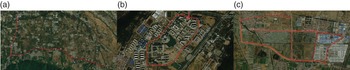
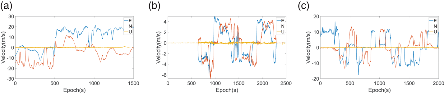
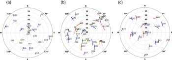
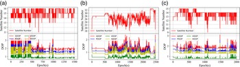
Experiment 1 was collected from 9:58:18 to 10:23:17 on 5 December 2017, on the G65 National Highway in the south of Chang'an District, Xi'an, China. Experiment 2 was collected from 03:17:40 to 03:59:01 on 28 March 2019. Vehicle dynamic experiment was carried out on the campus of China University of Mining and Technology (CUMT), Xuzhou, Jiangsu, China. Experiment 3 was also a vehicle-mounted dynamic experiment conducted in south of Tongshan District, Xuzhou, Jiangsu, China, which was collected from 08:48:15 to 09:21:34 on 15 July 2021. Figures 2 and 3 respectively show the reference trajectory with surroundings and vehicle speed of three experiments. As for the satellite sky plot, satellite number and dilution of precision (DOP) are shown in Figures 4 and 5.

Figure 2.

Reference trajectory of Experiment 1 (a), Experiment 2 (b) and Experiment 3 (c)

Figure 3.

Reference velocity of Experiment 1 (a), Experiment 2 (b) and Experiment 3 (c)

Figure 4.

Satellite sky plot of Experiment 1 (a), Experiment 2 (b) and Experiment 3 (c)

Figure 5.

Number of visible satellites and DOP of Experiment 1 (a), Experiment 2 (b) and Experiment 3 (c)

The experimental characteristics based on receiver velocity and observation environment are summarised. In Experiment 1, the vehicle speed and acceleration are high, and the vehicle is in an open environment, so this is the high speed open environment experiment. In Experiment 2, the vehicle speed is low, but there are tall buildings and trees on the campus. This is regarded as the low speed partial occlusion environment experiment. In Experiment 3, vehicle speed is high and its fluctuations are large, and the vehicle passes through industrial parks, greenhouses, and villages, an environment that contains large multipath effects. The configuration is considered to be a high speed partial occlusion environment.

In this section, for the purpose of verifying the proposed algorithm, three velocimetry methods are compared. TDCP I and TDCP II are the conventional TDCP method and Doppler enhanced TDCP approach based on ARKF, while TDCP III is the Doppler enhanced TDCP based on TARKF. All these methods are implemented in the open source software GAMP (Zhou et al., Reference Zhou, Dong, Li, Jiang, Wickert and Schuh2018).

4.2 High speed open environment

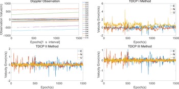
Figure 6 depicts the Doppler observation and velocity estimation results of three methods, and Table 1 describes the root mean square error (RMSE) of the three solutions.

Figure 6.

Doppler observation (upper left), estimated velocity by TDCP I (upper right), TDCP II (lower left) and TDCP III (lower right) in Experiment 1

Table 1.

RMSE of velocity estimated by TDCP I, TDCP II and TDCP III in Experiment 1

It can be seen from Table 1 that, compared with TDCP I, TDCP II improved the estimation accuracy of East (E), North (N), Up (U) and modulus by 24.77%, 27.70%, 86.42% and 56.56%. The high speed receiver may lead to cycle slip and measurement noise to carrier phase. Although the cycle slip detection algorithm can eliminate most cycle slips, there may be some tiny cycle slips that will reduce the quality of TDCP observations. Compared with the carrier phase observation, Doppler observation is more robust and will not be polluted by cycle slips, so modified TDCP can provide high-precision velocity. In addition, it should be noticed that the accuracy of U direction is improved significantly, and the RMSE obtained by TDCP II is even lower than the E and N directions. Just from the Equation (24), it can be concluded that using the modified TDCP observation can also apply the averaging of observations between epochs to smooth, further improving the velocity estimation accuracy.

TDCP II can improve the precision of velocity, but there are large errors between the estimation of velocity and reference value at some epochs. Although Doppler observation is used in TDCP II to approximate the instantaneous velocity, the solution is still based on displacement increment of time period. Therefore, ARKF is used to adjust the degree of matching between the prior state and measurement. However, the occurrence of errors indicates that the state update process may be inappropriate. Furthermore, after adopting the TARKF, compared with TDCP II, the precision in E, N, U and modulus are improved by 23.29%, 23.37%, –1.04% and 21.66%, respectively. Because the vehicle-mounted receiver travels on roads most of the time, these roads are completed by polynomials in the design and construction. TARKF just uses the historical state solution to fit this polynomial, thereby constraining the state update process. When the state update does not match the polynomial predicted state, the adaptive factor estimated by statistical test and Newton iteration method can be used which presented in section 3.3. Subsequently, the weight of prior state information is appropriately reduced, leading to the weight of observation being increased relatively, so that the estimation is more dependent on the observation.

4.3 Low speed partial occlusion environment

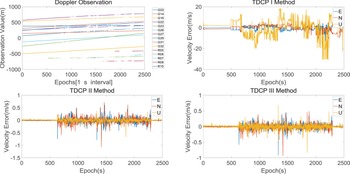
It was proved that the speed obtained by TDCP III has the highest accuracy, and the estimation accuracy of TDCP II is higher than that of TDCP I, as shown in section 4.2. The test is then conducted under low speed partial occlusion environment. The Doppler observation and estimated velocity results of approaches are shown in Figure 7, and the RMSEs are listed in Table 2. Because of the large number of satellites observed in Experiment 2, only part of the satellites' Doppler observation are listed.

Figure 7.

Doppler observation (upper left), estimated velocity by TDCP I (upper right), TDCP II (lower left) and TDCP III (lower right) in Experiment 2

Table 2.

RMSE of velocity estimated by TDCP I, TDCP II and TDCP III in Experiment 2

When the receiver is under high speed condition, or when the observation is blocked, it will reduce the quality of the carrier phase, causing low-precision TDCP observation. The TDCP I estimated velocity in Experiment 1 can still maintain sub-metre per second results, while the calculated speed in Experiment 2 is unable to meet the requirement of application, because the receiver is in a complex observation environment, which brings severe multipath effects. Under the influence of high speed, although cycle slip frequently occurs in the carrier phase observation, cycle slip detection can be used to eliminate and repair observations containing cycle slip. In an occluded environment, non-line-of-sight phenomena will erroneously increase the location distance included in the observation and seriously damage the estimation accuracy, so that cycle slip detection cannot be performed normally. In contrast, velocity measurement in an obscured environment is a greater challenge. Benefiting from the robustness of Doppler observation, after using TDCP II for speed estimation, the precision of E, N, U and modulus have been greatly improved, and the RMSE is all within 0.16 m/s. The RMSE of speed obtained in Experiment 2 is lower than that in Experiment 1, which also accords with the implication that the DOP of Experiment 2 is lower than the DOP of Experiment 1.

After applying TDCP III, accuracy of velocity is improved by 22.0%, 23.01%, −36.73% and 15.72% in E, N, U and modulus compared with TDCP II. This is because when performing TARKF, the adaptive factor reduces the overall weight of the prior state, which increases the credibility of observations. From Figure 5(b), horizontal dilution of precision (HDOP) is twice as large as vertical dilution of precision (VDOP). After increasing the credibility of observation, the RMSE for the horizontal direction and U direction also tends to be the relationship of twice. Another reason is that the adaptive factor reduces the overall weight of the prior state, which sometimes reduces the weight of high-precision prediction in U direction.

4.4 High speed partial occlusion environment

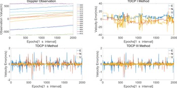
To verify the effect of the proposed algorithm under a high speed occlusion environment, the results obtained by using TDCP I, TDCP II and TDCP III methods are shown in Figure 8, and the RMSE is listed in Table 3. Because of the influence of multipath effects, TDCP I cannot provide available speed solutions. After using the TDCP II method, the RMSE can be controlled within 0.4 m/s in aspects of E, N, U and modulus. This shows that the TDCP II method can be applied to the velocity measurement of the receiver in an obscured environment, regardless of whether the receiver is at low speed or high speed.

Figure 8.

Doppler observation (upper left), estimated velocity by TDCP I (upper right), TDCP II (lower left) and TDCP III (lower right) in Experiment 3

Table 3.

RMSE of velocity estimated by TDCP I, TDCP II and TDCP III in Experiment 3

After using TDCP III, the accuracy in E, N, U and modulus can also be improved by 16.55%, 20.80%, –29.33%, and 15.57%. Moreover, there are still significant errors in this experiment. Through the analysis of experimental data, it is found that there are many observations with gross error. Therefore, it is necessary to use RKF to process the observations. However, RKF is only suitable for a few observations with gross error, that is, RKF needs redundant observations. Because this experiment only utilises GPS and GLONASS satellite data, sometimes the number of visible satellites is small, so observations with gross errors cannot be simply eliminated, resulting in large errors.