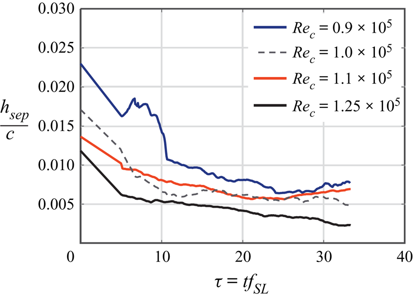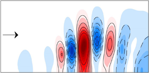



1. Introduction
A common goal of active flow control is to drive a particular flow state to a more favourable one with as little control effort as possible. This is often achieved by leveraging inherent flow instabilities (Greenblatt & Wygnanski Reference Greenblatt and Wygnanski2000). Active flow control can be employed, for example, to increase lift and reduce drag, enhance mixing for efficient combustion or for aeroacoustic noise attenuation (Gad-el Hak Reference Gad-el Hak2001; Williams & MacMynowski Reference Williams and MacMynowski2009; Brunton & Noack Reference Brunton and Noack2015). Due to the highly complex interactions inherent in fluid flows, modal decomposition approaches aid in the design and implementation of active flow control since the instabilities targeted often consist of discrete frequency, spatio-temporal coherent flow structures (modes) (Kutz et al. Reference Kutz, Brunton, Brunton and Proctor2016; Taira et al. Reference Taira, Brunton, Dawson, Rowley, Colonius, McKeon, Schmidt, Gordeyev, Theofilis and Ukeiley2017, Reference Taira, Hemati, Brunton, Sun, Duraisamy, Bagheri, Dawson and Yeh2019).
Most experimental flow control investigations employ parametric studies to identify an effective control approach for specified flow conditions (Seifert et al. Reference Seifert, Bachar, Koss, Shepshelovich and Wygnanski1993; Mittal, Kotapati & Cattafesta Reference Mittal, Kotapati and Cattafesta2005; Yarusevych, Kawall & Sullivan Reference Yarusevych, Kawall and Sullivan2006; Raju, Mittal & Cattafesta Reference Raju, Mittal and Cattafesta2008; Griffin et al. Reference Griffin, Oyarzun, Cattafesta, Tu, Rowley and Mittal2013). However, the parameter space for such an optimization can quickly become prohibitive. To aid in the control-design process, physical intuition can sometimes be leveraged to identify appropriate parameters. Furthermore, recent progress in optimal disturbance theory and constrained optimization provides additional mathematical tools for implementation of active flow control (Cossu Reference Cossu2014; de Pando, Schmid & Sipp Reference de Pando, Schmid and Sipp2017). However, the flow control approaches described above are open loop and designed for a specific uncontrolled baseline flow. Depending on the nature of the flow, these approaches may not be robust to deviations in the flow conditions. This can result in poor performance when control is employed at off-design conditions or when significant disturbances are present. Robustness is improved by implementing closed-loop control, which can be either model free or can incorporate estimates of the underlying dynamics.
Common model-free closed-loop control approaches include extremum and slope-seeking feedback control (Ariyur & Krstic Reference Ariyur and Krstic2003), employing gradient-descent algorithms that seek local extrema based on the response of the system output to slow input sinusoidal perturbations. These approaches have been utilized in separation control studies (Becker et al. Reference Becker, King, Petz and Nitsche2007; Benard et al. Reference Benard, Moreau, Griffin and Cattafesta2010). An alternate model-free approach employs downhill simplex optimization to estimate the control parameters for maximizing the time-averaged lift-to-drag ratio of an airfoil (Cattafesta, Tian & Mittal Reference Cattafesta, Tian and Mittal2009). More recently, methods from machine learning have been employed in flow control, in which the control design is framed as a regression problem and solved by genetic algorithms without explicit knowledge of the dynamics (Duriez, Brunton & Noack Reference Duriez, Brunton and Noack2017; Li et al. Reference Li, Noack, Cordier, Boree and Harambat2017; Wu Reference Wu2018). Unfortunately, by design, current model-free approaches exhibit slow learning and adaptation times relative to the fluid dynamic time scales.
Model-based, closed-loop control approaches are designed based on dynamical models of the flow and circumvent learning times associated with their model-free counterparts. Conventional closed-loop control approaches usually involve linear estimates of the underlying dynamics and utilize feedback to drive the system to a desired state. One challenge with model-based approaches in flow control is that the dynamics may vary significantly with initiation of control. Therefore, such approaches generally require incorporating knowledge of a wide range of input/output dynamics. Dynamical models can be identified by input/output parameter sweeps using system identification techniques (neural network, ARMARKOV, etc.) (Platt Reference Platt1991; Akers & Bernstein Reference Akers and Bernstein1997; Reese et al. Reference Reese, Collins, Fernandez and Alvi2016). Alternatively, a probabilistic approach can be adopted to model and control fluid flows, such as cluster-based reduced-order modelling (Kaiser et al. Reference Kaiser, Noack, Cordier, Spohn, Segond, Abel, Daviller, Östh, Krajnović and Niven2014, Reference Kaiser, Noack, Spohn, Cattafesta and Morzyński2017). Reduced-order dynamical models can also be derived from the underlying flow physics using a Galerkin projection (Noack, Morzynski & Tadmor Reference Noack, Morzynski and Tadmor2011). However, Galerkin models, particularly those accessible via physical experiments, are often susceptible to numerical instability and become invalid if the system moves far from its uncontrolled base state.
Regardless of the modelling approach, the complex dynamics inherent in fluid flows generally yields significant changes in the coherent structures and stability characteristics under external forcing, possibly invalidating the model used for closed-loop control. This difficulty is exacerbated by the fact that flow control is implemented to drive the flow to a more desirable state that is significantly different than the uncontrolled baseline state. Therefore, an effective closed-loop control strategy should ideally implement some form of adaptation that quickly updates the dynamics in order to properly track deviations from the baseline.
These issues give rise to several technical challenges for model-based closed-loop control that responds on the same order as the time scales of the fluid system. First, an appropriate sensing approach needs to be implemented to permit accurate estimation of the relevant dynamical states with limited sensors. Second, the actuator must have sufficient bandwidth and time response to ensure that it can excite the appropriate modes of the flow and respond rapidly to broadband control signals. Third, an accurate yet simple reduced-order model of the underlying fluid dynamics is required to enable adaptation to time-varying dynamics or flow conditions. Finally, an appropriate feedback controller must be designed and implemented. While a general approach is currently not in place to address these concerns, this work offers a potential solution for the specific example of adaptive, closed-loop control of a laminar separation bubble (LSB) using online dynamic mode decomposition (DMD) with control.
A pressure-gradient-induced LSB forms when a laminar boundary layer detaches from a wall to form a shear layer due to a sufficiently strong adverse pressure gradient, undergoes transition and ultimately reattaches downstream to form a closed bubble. LSBs may develop on laminar airfoils (Joslin Reference Joslin1998), low-pressure turbine blades (Hodson & Howell Reference Hodson and Howell2005), small aerial vehicles (Mueller & DeLaurier Reference Mueller and DeLaurier2003) and wind-turbine blades (Sørensen Reference Sørensen2011) and, in nearly all cases, have a detrimental effect on performance.
LSBs have been extensively studied for decades. Briefly, Gaster (Reference Gaster1966) rigorously examined the dynamics of pressure-induced LSBs on a semi-infinite flat plate without the additional complications of curved geometry and proposed a bursting criterion to predict when a short bubble changes to a much longer one. Marxen & Henningson (Reference Marxen and Henningson2011) described the complex physics associated with LSBs, such as the convective amplification of high-frequency disturbances in the shear layer due to the Kelvin–Helmholtz instability. They also offered distinguishing features between short and long bubbles, further examining the mechanisms of bubble bursting in which vortex shedding ceases and low-frequency flapping may occur. As a precursor to control, Michelis, Yarusevych & Kotsonis (Reference Michelis, Yarusevych and Kotsonis2017) examined the response of a LSB to impulsive two-dimensional (2-D) forcing with dielectric barrier discharge actuators and found that impulsive forcing produces a wave packet, associated with rapid shrinkage of the bubble in both upstream and downstream directions, with properties that are in remarkable agreement with linear stability analysis. Their results supported earlier work (Rist & Augustin Reference Rist and Augustin2006; Marxen & Risk Reference Marxen and Risk2010) that the disturbance input results in a global change of the pressure gradient due to mean-flow deformation and drives the bubble towards a more stable state.
Collectively, the prior work indicates that active control of the instabilities can provide effective control. Indeed, many studies have been conducted in which actuation parameters are varied, and the performance is evaluated a posteriori (Seifert, Darabi & Wyganski Reference Seifert, Darabi and Wyganski1996; Seifert & Pack Reference Seifert and Pack1999; Glezer, Amitay & Honohan Reference Glezer, Amitay and Honohan2005; Mittal & Kotapati Reference Mittal and Kotapati2006; Raju et al. Reference Raju, Mittal and Cattafesta2008). Several studies aimed at determining an optimal forcing frequency suggest forcing at the most amplified shear-layer instability frequency results in significant flow separation mitigation (Yarusevych et al. Reference Yarusevych, Kawall and Sullivan2006; Postl, Balzer & Fasel Reference Postl, Balzer and Fasel2011; Marxen et al. Reference Marxen, Kotapati, Mittal and Zaki2015; Yarusevych & Kotsonis Reference Yarusevych and Kotsonis2017). As noted above, the very goal of reducing the size of a separation bubble by unsteady actuation means that the base state of the separated flow will undergo significant deformation that will alter the instability characteristics (Marxen et al. Reference Marxen, Kotapati, Mittal and Zaki2015). This scenario motivates adaptive closed-loop separation control in which the dynamical model of the separated flow is updated automatically as actuation is applied.
However, adaptive closed-loop separation control introduces additional complexities related to dynamical model derivation, objective function specification and state measurement and estimation. Our previous work shows that DMD accurately emulates the oscillatory characteristics of a separated flow (Deem et al. Reference Deem, Cattafesta, Zhang, Rowley, Hemati, Cadieux and Mittal2017; Hemati et al. Reference Hemati, Rowley, Deem and Cattafesta2017). DMD was recently introduced in fluid dynamics for identifying spatially coherent flow structures from a set of either experimental or simulation snapshot observations of various flow quantities (Rowley et al. Reference Rowley, Mezić, Bagheri, Schlatter and Henningson2009; Schmid Reference Schmid2010). In this context, DMD provides a transition matrix that is a linear estimate of the mapping between a current snapshot and the next snapshot in time. For the cases in which external forcing is acting on the dynamical system, such as with the zero-net mass-flux (ZNMF) actuator upstream of separation in the present work, the conventional DMD algorithm can be modified to incorporate actuation (Proctor, Brunton & Kutz Reference Proctor, Brunton and Kutz2016). The dynamic modes are then the eigenvectors of the identified linear transition matrix. Since this flow dynamics is typically described well by a low-dimensional subspace, rank-reduction techniques can be performed to express a low-order representation of the dynamics with a small set of dynamically relevant modes (Rowley et al. Reference Rowley, Mezić, Bagheri, Schlatter and Henningson2009; Schmid Reference Schmid2010; Hemati et al. Reference Hemati, Rowley, Deem and Cattafesta2017).
In order to leverage this capability in an adaptive, closed-loop control setting, a new algorithm known as online DMD is employed, which efficiently updates the linear transition model with control provided by DMD as soon as a new state measurement is available (Deem et al. Reference Deem, Cattafesta, Zhang, Rowley, Hemati, Cadieux and Mittal2017, Reference Deem, Cattafesta, Huaijin, Hemati, Zhang and Rowley2018; Zhang et al. Reference Zhang, Rowley, Deem and Cattafesta2019). Therefore, the variations in the dynamics are represented as a time-varying linear system. Given a sufficiently small number of sensors, this update step can be done at a rate that is faster than the characteristic frequencies of the flow, allowing for real-time dynamical system estimates. For the current study, the measurements used to identify the discrete linear model provided by online DMD are unsteady surface pressure snapshots taken by a linear array of thirteen surface-mounted microphones. This rapidly adapting linear system captures both the modal structure of the flow and the transient evolution of the modes as actuation is applied or as flow conditions change in real time. Using the linear model provided by online DMD, standard linear optimal control methods are shown to be viable for autonomous control of separated flow.
The control approach implemented in this study consists of rapidly updating feedback gains from a linear quadratic regulator (LQR) process as the linear system estimate is updated by online DMD. In general, the resulting feedback control is not expected to be optimal per se since the underlying dynamics is not linear and time invariant. However, this is the set of optimal feedback gains for the current dynamical estimate. Due to the computational requirements to solve the discrete algebraic Riccati equation, the LQR feedback gain update rate is slower than the online DMD update rate, but still sufficiently faster than the characteristic flow frequency. The resulting response of the flow to control is characterized by time-resolved particle image velocimetry (PIV) and unsteady pressure measurements.
The next sections provide a detailed description of the experimental apparatus and computational methods used in this work (§§ 2–4), followed by analysis of the baseline separated flow characteristics in § 5. In § 6, the response of the separated flow to open-loop control using periodic burst modulation is evaluated for varying modulation frequency and actuator momentum coefficients to demonstrate the receptivity of the flow to this actuation approach and to provide open-loop control results to compare with the adaptive control approach. Then, the results of applying adaptive closed-loop separation control are provided for varying actuator penalty parameters in § 7. For comparison, control is applied using a non-adaptive offline-identified dynamical model. For each case, running calculations of various turbulence quantities and pressure fields are presented to identify the evolution of these quantities after control is initiated, and the results are discussed. The transient evolution of natural reattachment is evaluated by deactivating the imposed adverse pressure gradient. The turbulence and pressure-field quantities for this case of natural reattachment are presented and compared to those corresponding to reattachment by adaptive closed-loop control. Finally, to demonstrate the robustness of this approach to varying flow conditions, control is applied for varying Reynolds number.
2. Experimental set-up
This experimental study utilizes the canonical separated flow configuration described in Griffin et al. (Reference Griffin, Oyarzun, Cattafesta, Tu, Rowley and Mittal2013), Hemati et al. (Reference Hemati, Deem, Williams, Rowley and Cattafesta2016) and Deem et al. (Reference Deem, Cattafesta, Zhang, Rowley, Hemati, Cadieux and Mittal2017) and is motivated by the work of Na & Moin (Reference Na and Moin1998) to remove curvature dependencies on boundary layer separation. Here, a laminar boundary layer on a flat plate model separates due to an adverse pressure gradient imposed by siphoning a portion of the free-stream flow through the ceiling of the wind tunnel test section and reinjecting it just downstream. This section provides details regarding the experimental design, data collection, real-time control system and the methods used for processing and analysing the results.
2.1. Wind tunnel facility and experimental model
Experiments were conducted in the Florida State Flow Control (FSFC) open-return wind tunnel facility. The FSFC wind tunnel has a 9 : 1 inlet contraction and a square 30.5 cm test section with a length of 61.0 cm. Upstream of the contraction, flow conditioning is accomplished by a honeycomb mesh and two anti-turbulence mesh screens. The free-stream turbulence intensity integrated above 4 Hz is  $u'/U_\infty = 0.5\,\%$. The flat plate model used in this study spans the entire width of the test section, has chord dimension
 $c = 40.2$ cm and thickness
 $w = 0.095c$. The leading edge of the plate is a 4 : 1 ellipse, and the trailing edge is square. A pitot-static probe mounted upstream of the model monitors the free-stream velocity, which is maintained at
 $U_\infty = 3.9 \pm 0.1$ m s
 $^{-1}$ via a proportional-integral-derivative controller to provide a chord Reynolds number of
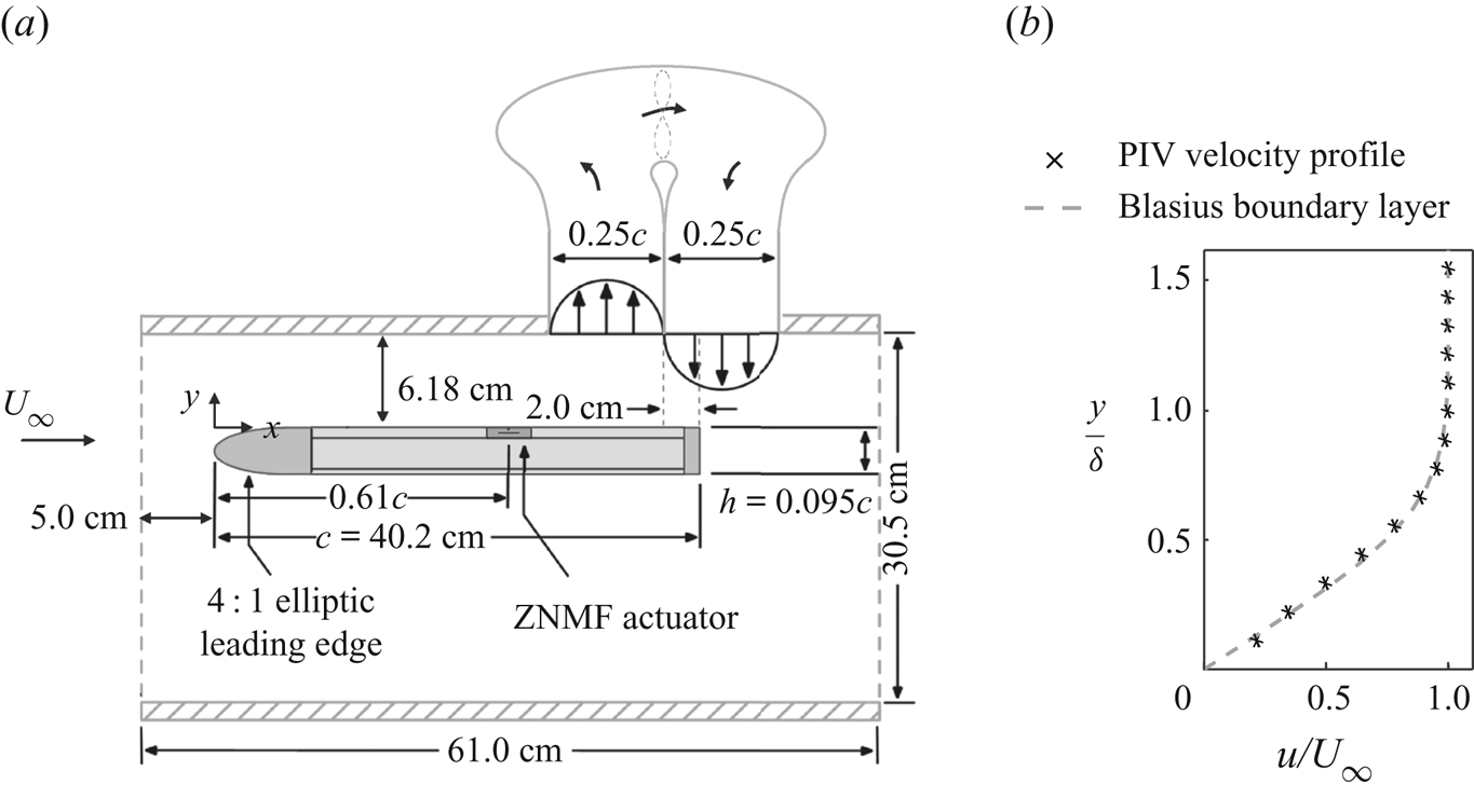
 $Re_c = 10^5$. A schematic of the plate with relevant dimensions is shown in figure 1(a).
(a) Schematic of the flat plate model and flow separation system. (b) Mean velocity profile upstream of the separation point extracted by PIV measurements. The Blasius laminar boundary layer solution is plotted for reference.  $x/c \approx 0.3$. (a) Experimental set-up and (b) upstream boundary layer profile.

A ZNMF suction/blowing tunnel ceiling boundary condition is imposed to induce boundary layer separation on the top surface of the flat plate. A Mechatronics Inc. MM28080H dc motor driven fan ingests a portion of the free-stream fluid through an acoustically treated perforated plate segment of the test section ceiling and then injects this flow back into the test section through a return duct that is similarly acoustically treated. The ratio of the average suction/blowing velocity to that of the free stream is  $0.16 \pm 0.03$.
The set-up is designed to allow for the location and extent of the separation bubble to vary by changing the location of the plate with respect to the ceiling duct. For the current case, as discussed further below, a closed separation bubble is generated that exhibits mean reattachment upstream of the trailing edge of the flat plate. The spanwise uniformity of the separation region is assessed by surface flow visualization and PIV. The separation point is estimated by PIV for several spanwise locations, subject to optical access. From these data, the variation in the separation and reattachment locations along the central 70 % of the span exhibit a maximum deviation of 3 % chord.
The mean velocity profile upstream of the separation point is extracted from 4800 PIV snapshots and is plotted along with the Blasius boundary layer profile in figure 1(b) with a spatial resolution of  ${\rm \Delta} x = 0.466$ mm. The boundary layer thickness is
 $\delta = 3.7$ mm, and the shape factor is estimated as
 $H = 2.67 \pm 0.08$ at
 $x/c \approx 0.3$. Comparing this to
 $H = 2.59$ for the Blasius boundary layer indicates that the boundary layer is laminar upstream of separation and is subjected to a small favourable pressure gradient due to the growing turbulent boundary layers on the wind tunnel walls.
2.2. Actuation
A rectangular slot ZNMF actuator is employed to force the separated flow. The ZNMF jet sequentially ingests and expels surrounding fluid by varying the volume of a cavity underneath the slot (Glezer & Amitay Reference Glezer and Amitay2002; Cattafesta & Sheplak Reference Cattafesta and Sheplak2011). Thus, there is zero time-average mass flux but a non-zero momentum flux. The actuator orifice is 2 mm wide, is located upstream of the separation location at  $x/c = 0.61$ (the mean baseline separation location is
 $x/c = 0.70$), and spans the central 58
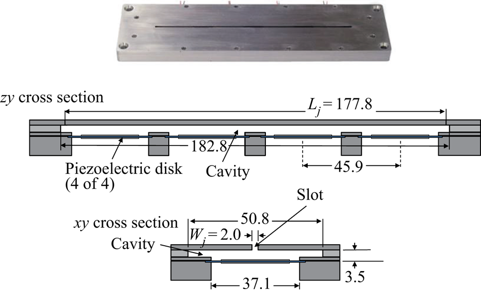
 $\%$ of the model. The actuator is comprised of four bimorph piezoelectric disks (APC Inc., PZT5J, Part Number: P412013T-JB) that serve to vary the volume of the cavity as an ac voltage is applied across the disks. The disks are mounted spanwise along the lower surface of the cavity, and are numbered increasing from right to left (relative to the free-stream direction). The schematic of the actuator in figure 2 shows relevant actuator dimensions.
Photograph and schematic illustration of the ZNMF actuator (adapted from Griffin et al. Reference Griffin, Oyarzun, Cattafesta, Tu, Rowley and Mittal2013). Dimensions are in mm.  $L_j$ is the length of the actuator slot and
 $W_j$ is the width of the actuator slot. The height of the actuator orifice is
 $H_j = 2$ mm.

The disks are driven by a high-frequency sine wave, modulated down to the natural frequency range of the current separated flow. The choice of the high-frequency carrier frequency is discussed in the next section. The actuator output is expressed in terms of the momentum coefficient ( $C_\mu$), which is defined as
 \begin{equation} C_\mu = \frac{A_j \bar{v}^2_{rms}}{A_{sep}U^2_{\infty}}. \end{equation}
In this definition,  $A_j = W_j\times L_j$ is the area of the actuator slot, and the separation area is the baseline uncontrolled length of the mean separation region multiplied by
 $S$, which is the span of the plate (
 $A_{sep} = L_{sep}\times S$). The velocity across the jet orifice is measured by PIV during control experiments. For the actuator PIV measurements, the root-mean-square (r.m.s.) velocity directly adjacent to the actuator orifice is spatially averaged over the slot width to quantify the velocity fluctuations (
 $\bar {v}_{rms}$) through the actuator.
2.3. Actuator characterization
Prior to conducting experiments, the output of the actuator is first determined when driven by a sinusoid with various forcing frequencies and amplitudes. For characterization, the r.m.s. velocity of the actuator is determined by constant-temperature hot-wire anemometry, in which the hot-wire probe is placed at the centre of the actuator slot above Disk 1. A Dantec 55P11 hot-wire probe with a wire diameter of 5  $\mathrm {\mu }$m and length of 1.25 mm is used. The hot-wire probe is calibrated before and after the actuator characterization for a velocity range of 0 to 30 m s
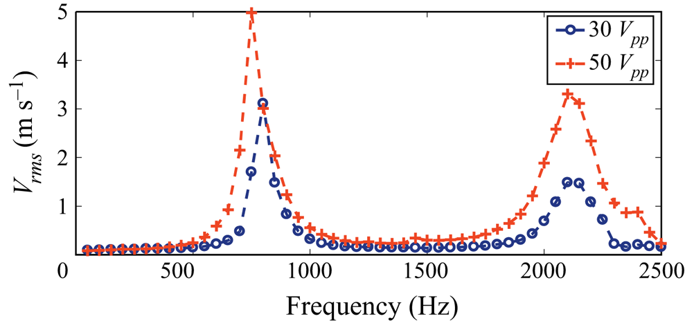
 $^{-1}$, and a fourth-order polynomial is fit to the calibration data. The hot-wire signal is sampled at 20 480 Hz with a National Instruments PXI-4462 data acquisition card. Figure 3 shows the
 $V_{rms}$ response from the hot-wire probe centred above Disk 1 when driving all four disks simultaneously. The frequency is stepped by 50 Hz from 50 to 2500 Hz. This test is repeated for two input amplitudes of 30 and 50
 $V_{pp}$.
Velocity frequency response for driving amplitudes of 30 and 50  $V_{pp}$ in the slot centre above Disk 1.

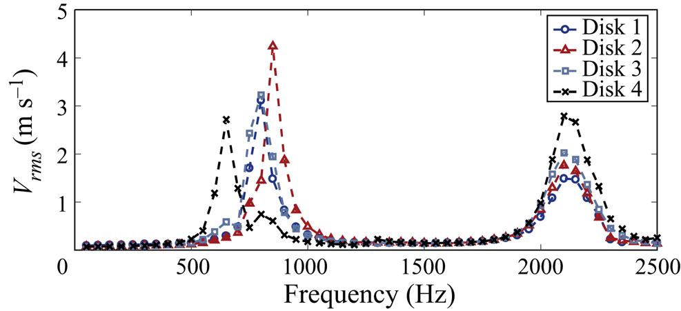
The hot-wire probe is then centred above the other three disks, and this test is repeated for an input amplitude of 30  $V_{pp}$. Figure 4 provides the
 $V_{rms}$ responses for centring the hot-wire probe above each disk.
Velocity frequency responses in slot centre above all four disks for a driving amplitude of 30  $V_{pp}$.

These figures show two distinct resonant peaks at the Helmholtz frequency of the cavity (near 700 Hz) and the diaphragm resonance frequency (2100 Hz). Noting the output of the actuator is negligible below  $\sim$500 Hz when driven by a sinusoid, a burst-modulated (i.e. square-wave modulated) signal is selected to augment the output at low frequencies. While the largest output can be produced by selecting a carrier frequency close to the Helmholtz frequency, this approach is avoided because of the large acoustic pressure fluctuations that corrupt the unsteady surface pressure sensor measurements (Griffin Reference Griffin2013). Therefore, the carrier frequency is chosen to be slightly below the diaphragm resonance frequency at
 $f_c = 2050$ Hz to produce reasonable output while avoiding inevitable phase variations in diaphragm motion associated with driving the actuators at a mechanical resonance frequency. This choice also reduces the risk of actuator damage.
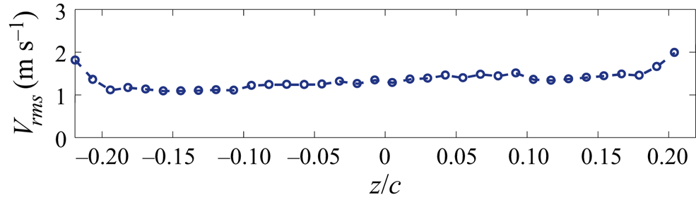
The spanwise uniformity of the actuator is addressed by traversing the hot wire along the length of the slot while driving the actuator with a single sine wave at a frequency of  $f_c = 2050$ Hz and amplitude of 30
 $V_{pp}$. The r.m.s. velocity measured for varying span is provided in figure 5. The actuator output variation is within 16 % for the central 84 % of the actuator slot. At the extreme edges of the actuator slot, the maximum variation increases to 51 %.
The spanwise variation of the r.m.s. velocity as measured by a hot-wire probe for a  $2050$ Hz sine wave driving signal at 30
 $V_{pp}$.

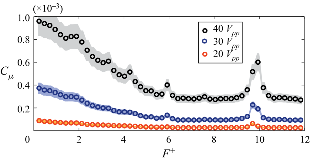
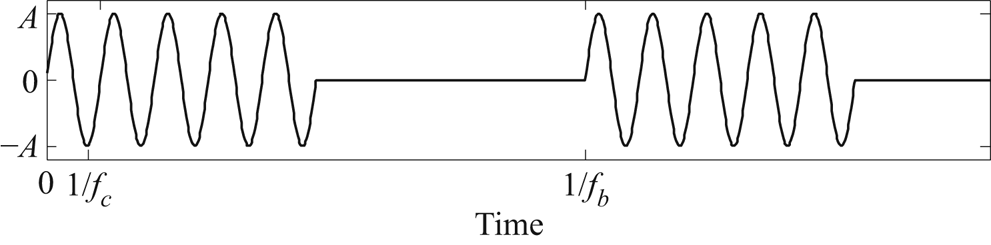
The momentum coefficient of the ZNMF jet actuator subject to a burst modulation drive signal, illustrated in figure 6, is plotted for varying modulation frequencies, in which  $f_b$ is stepped by 10 Hz. The shaded region depicts the 95 % confidence intervals in
 $C_\mu$. For the burst modulated waveform, the carrier frequency (
 $f_c$) sine wave is cycled on and off at the burst frequency
 $f_b$. The nominal duty cycle of the modulation is set to 50 %. However, in order to prevent spectral leakage and unanticipated high-frequency content, the duty cycle can vary slightly from this value to ensure that an integer number of carrier cycles exists within the burst period. The forcing frequency is non-dimensionalized with respect to the baseline separation bubble length and free-stream velocity as
 \begin{equation} F^+ = \frac{f_bL_{sep}}{U_\infty}. \end{equation}
Momentum coefficient with respect to varying forcing frequencies. The 95 % confidence intervals are depicted by the shaded region.

2.4. Unsteady pressure sensors
The unsteady pressure on the model surface is measured by an array of 13 flush-mounted Panasonic WM-61A electret microphones. The diameter of the exposed microphone diaphragm of the WM-61A microphones is 2 mm, and the microphones are mounted in the mid-span plane from  $x/c=0.7$ to
 $x/c=0.94$ in increments of
 $x/c = 0.02$. The microphones are powered by a 4 mA constant current source provided by an NI PXI-4498 data acquisition card.
Previous work has shown that the microphones employed in this study are sensitive to signal contamination from extraneous acoustic sources (Griffin Reference Griffin2013; Deem et al. Reference Deem, Cattafesta, Zhang, Rowley, Hemati, Cadieux and Mittal2017). Contaminating sources include the acoustic signal generated by the actuator, the wind-tunnel fan, and the separation-duct fan. One potential remedy for this is to perform conditioned spectral analysis to remove the contaminating signals and account for mutual contamination a posteriori (Bendat & Piersol Reference Bendat and Piersol2011, Reference Bendat and Piersol2013; Deem et al. Reference Deem, Cattafesta, Zhang, Rowley, Hemati, Cadieux and Mittal2017). However, for real-time control, any contaminants must be filtered in a manner that is realizable within the primary control loop. This study incorporates analogue low-pass filters in addition to digital filters within the control loop to remove unwanted high-frequency content and also ac couple the signals. The filtered signals are digitized by an NI PXIe-6358 card at a rate of 10 kHz. Furthermore, two additional reference microphones are mounted near the separation-duct fan and on the floor of the wind tunnel to measure the coherence function between each reference microphone and the surface mounted microphones, thus enabling us to determine the severity of signal contamination.
2.5. Time-resolved PIV
Both the separated flow and actuator slot regions are synchronously measured by time-resolved particle image velocimetry (TR-PIV). The laser sheet is oriented in the  $x$–
 $y$ plane, slightly offset from mid-span with its optical axis parallel to the surface in order to reduce reflections. The camera field of view has a streamwise extent from
 $x/c \approx 0.62$ to
 $x/c \approx 1$ and a height of
 $y/c \approx 0.13$. Within the same plane, the actuator PIV region is bounded by
 $x/c \approx 0.59$ and
 $x/c \approx 0.63$, and has a height of
 $y/c = 0.087$. Olive oil droplets with nominal diameter of 1
 $\mathrm {\mu }$m introduced to the flow from a TSI 9307-6 atomizer are used for PIV seed particles (Melling Reference Melling1997). The particles are illuminated by a high rep rate Nd-YAG laser operating in a single pulse configuration and images of the illuminated particles are acquired by a Phantom v1611 high speed camera. For the baseline uncontrolled flow, the actuator slot is open, and the resolution of the images is
 $1280 \times 800$ pixels. Images are acquired at 5 kHz for at least 4800 frames. In this case, the velocity vector fields are computed in between each image, so the effective PIV sample rate is 5 kHz. Once images are acquired, image preprocessing and vector calculations are performed using LaVision DaVis 8.4.0. A multi-pass cross-correlation algorithm is used to determine the velocity vectors. The initial interrogation window size is
 $64 \times 64$ pixels, and the final interrogation window size is
 $24 \times 24$ pixels with 75
 $\%$ overlap resulting in a vector spacing of 0.73 mm.
For the control cases, the PIV images are acquired at a sample rate of 10 kHz to enable synchronous measurements with the real-time control system. In this case, the final interrogation window size is reduced to  $16 \times 16$ pixels with 75
 $\%$ overlap resulting in a vector spacing of 0.49 mm. The final interrogation window size of the higher magnification actuator measurement region is
 $32 \times 32$ pixels with 75 % overlap, resulting in a vector spacing of 0.18 mm or approximately 11 measurement locations across the actuator slot.
In all cases, post-processing steps are as follows. Multivariate outlier rejection is first employed to identify and eliminate outliers in each velocity field snapshot using the method in Griffin et al. (Reference Griffin, Schultz, Holman, Ukeiley and Cattafesta2010). The velocity data are low-pass filtered (with a cutoff frequency of not less than 500 Hz) to remove high-frequency noise. Finally, the gappy proper orthogonal decomposition (POD) method described in Saini, Arndt & Steinberg (Reference Saini, Arndt and Steinberg2016) is used to replace missing vectors to enable estimation and analysis of instantaneous quantities, such as spanwise vorticity and pressure from PIV. The uncertainty in each vector field measurement is calculated using the correlation-statistics method for estimating PIV uncertainty (Wieneke Reference Wieneke2015). In order to propagate the uncertainty in each PIV vector to the various calculated quantities referred to in this work, standard linear uncertainty propagation is employed. See Deem (Reference Deem2018) for details regarding the estimation of uncertainties with 95 % confidence for this study, including the treatment of error correlation due to PIV interrogation window overlap. The maximum uncertainty in the mean  $u$-velocity and
 $v$-velocity is approximately 0.5 % and 0.4 % of
 $U_\infty$, respectively. The largest uncertainty in the mean vorticity is 2 % of the maximum value of vorticity. The height of the separation region is also estimated from the PIV results. The uncertainty in the separation height for the baseline flow is approximately 0.5 %.
2.6. Real-time control hardware
An NI PXIe-8880, a 2.3 GHz Intel Xeon 8-Core embedded controller, is employed for state measurement, online model estimation, feedback gain calculation and actuation signal generation. The microphone signals are filtered by eight KEMO VFBF35 and five Stanford Research model SR640 programmable low-pass filters and then simultaneously sampled by an NI PXIe-6358 data acquisition card connected to the real-time controller.
NI Veristand 2017 is used to develop the control-loop software. Online DMD (described below) is coded in Simulink. A built-in discrete linear quadratic regulator (LQR) function from LabVIEW 2017 is used to calculate the LQR gains given the current system estimates from online DMD. Finally, a code for generating the actuator signal is developed in Simulink. The analogue output signal to the actuator is produced by the NI PXIe-6358 card and routed to a Trek PZD350 external amplifier and then to the piezoceramic disks. Once all of these codes are compiled and appropriately mapped in Veristand, the final program is executed at a specified sample rate on the real-time controller.
3. Dynamic mode decomposition
For the current study, variants of DMD are employed for baseline flow analysis and state-space model identification for real-time control. Given many simultaneously sampled measurements of a particular dynamical process, DMD provides a finite-dimensional discrete-time linear system that approximates the Koopman operator (an infinite-dimensional linear description for nonlinear dynamical systems) that evolves the dynamics one time step forward (Rowley et al. Reference Rowley, Mezić, Bagheri, Schlatter and Henningson2009; Schmid Reference Schmid2010; Tu et al. Reference Tu, Rowley, Luchtenburg, Brunton and Kutz2014; Williams, Kevrekidis & Rowley Reference Williams, Kevrekidis and Rowley2015).
The snapshot measurement vectors are denoted as  $\boldsymbol {x_k}$. The transition matrix is denoted
 $\boldsymbol{\mathsf{A}}_{DMD}$ and satisfies the approximate relation
 \begin{equation} \boldsymbol{x_{k+1}} \approx \boldsymbol{\mathsf{A}}_{DMD} \boldsymbol{x_{k}}.\end{equation}
Snapshot matrices are constructed from sequences of snapshot data column vectors as
 \begin{equation} \boldsymbol{\mathsf{X}} = \begin{bmatrix} | & | & & | \\ \boldsymbol{x}_1 & \boldsymbol{x}_2 & \cdots & \boldsymbol{x}_{n-1}\\ | & | & & | \end{bmatrix}, \quad \boldsymbol{\mathsf{Y}} = \begin{bmatrix} | & | & & | \\ \boldsymbol{x}_2 & \boldsymbol{x}_3 & \cdots & \boldsymbol{x}_{n}\\ | & | & & | \end{bmatrix}.\end{equation}
The previous snapshot matrix is denoted by  $\boldsymbol{\mathsf{X}}$, and the current snapshot matrix (denoted by
 $\boldsymbol{\mathsf{Y}}$) is the previous snapshot matrix shifted forward by one time step. Each snapshot vector consists of
 $\boldsymbol {m}$ simultaneous measurements, and a total of
 $\boldsymbol {n}$ snapshots are recorded. The snapshot matrices thus have dimension
 $\boldsymbol {m} \times (\boldsymbol {n}-1)$.
The DMD transition matrix can be determined by multiplying the current snapshot matrix with the pseudoinverse (denoted by  $^+$) of the previous snapshot matrix (Tu et al. Reference Tu, Rowley, Luchtenburg, Brunton and Kutz2014)
 \begin{equation} \boldsymbol{\mathsf{A}}_{DMD} := \boldsymbol{\mathsf{Y}}\boldsymbol{\mathsf{X}}^+.\end{equation}
In practice, a reduced problem is formulated by taking the singular value decomposition (SVD) of the snapshot matrix  $\boldsymbol{\mathsf{X}} = \boldsymbol{\mathsf{U}}\boldsymbol {\Sigma } \boldsymbol{\mathsf{V}}^*$, in which
 $^*$ denotes the complex conjugate transpose. This result is substituted into (3.3) to yield
 \begin{equation} \boldsymbol{\mathsf{A}}_{DMD} = \boldsymbol{\mathsf{Y}}[\boldsymbol{\mathsf{U}}\boldsymbol{\Sigma} \boldsymbol{\mathsf{V}}^*]^+ = \boldsymbol{\mathsf{Y}}\boldsymbol{\mathsf{V}}\boldsymbol{\Sigma}^+ \boldsymbol{\mathsf{U}}^* . \end{equation}
DMD modes and eigenvalues are then related to the eigenvectors and eigenvalues of  $\boldsymbol{\mathsf{A}}_{DMD}$. The number of DMD modes and eigenvalues will be
 $min (\boldsymbol {m},\boldsymbol {n}-1)$. A modal truncation can be performed, if it is expected that
 $r<min (\boldsymbol {m},\boldsymbol {n}-1)$ modes are required to capture the important dynamics. This is achieved by truncating the SVD of
 $\boldsymbol{\mathsf{X}}$ to include only the first
 $r$ singular values and associated left and right singular vectors, in which a subscript
 $r$ will denote a truncated matrix. From this, the reduced proxy system matrix can be determined by
 \begin{equation} \tilde{\boldsymbol{\mathsf{\!\!A}}} = \boldsymbol{\mathsf{U}}_r^*\boldsymbol{\mathsf{A}}_{DMD}\boldsymbol{\mathsf{U}}_r =\boldsymbol{\mathsf{U}}^*_r\boldsymbol{\mathsf{Y}}\boldsymbol{\mathsf{V}}_r \boldsymbol{\Sigma}^+_r . \end{equation}
The non-zero DMD eigenvalues are given by  $\lambda _i$, and are computed as the eigenvalues of
 $\ \tilde {\boldsymbol{\mathsf{\!\!A}}}$. The DMD modes are computed by
 $\boldsymbol {\phi }_i = \boldsymbol{\mathsf{U}}_r\boldsymbol {w}_i$ in which
 $\boldsymbol {w}_i$ is the
 $i$th eigenvector of
 $ \tilde {\boldsymbol{\mathsf{\!\!A}}}$. The frequency and growth rate for the
 $i$th mode are
 $f_i = f_s \angle \lambda _i/(2 {\rm \pi})$ and
 $g_i = f_s \log |\lambda _i|$.
DMD analysis of results derived from PIV measurements in this study are also computed using the noise-robust total-least-squares DMD (TDMD) algorithm presented in Hemati et al. (Reference Hemati, Rowley, Deem and Cattafesta2017). The TDMD procedure consists of a preprocessing step that removes the asymmetric treatment of measurement noise inherent in the formulation of DMD provided above (Dawson et al. Reference Dawson, Hemati, Williams and Rowley2016; Hemati et al. Reference Hemati, Rowley, Deem and Cattafesta2017). Furthermore, the TDMD is combined with the sparsity-promoting DMD approach of Jovanović, Schmid & Nichols (Reference Jovanović, Schmid and Nichols2014) to enable a systematic study of the trade-off between the quality of approximation and the number of modes that are used. We refer to this combination as ‘SP-TDMD’.
The oscillatory amplitude of the estimated DMD modes are of primary interest in the control approach described later. As such, we determine the contribution of each DMD mode to each snapshot using  $ \tilde {\boldsymbol{\mathsf{\!\!A}}}$ and then compute the mean-squared value of each mode, first in space for each snapshot and then in time for all snapshots, and normalize the result by the maximum value to obtain a linear estimate of the relative importance of the
 $i$th mode, denoted as
 ${\sigma _{DMD,i}^2}$. The overall quality of the DMD analysis is compared to the space–time POD using the spectral proper orthogonal decomposition (SPOD) algorithm of Towne, Schmidt & Colonius (Reference Towne, Schmidt and Colonius2018), noting that the space–time POD is not currently amenable to the online DMD used for estimation and control.
However, this may be possible in the future through variations on the streaming SPOD algorithm (Schmidt & Towne Reference Schmidt and Towne2019).
3.1. Online DMD
The DMD formulation provided above requires that every snapshot of  $\boldsymbol{\mathsf{X}}$ be readily available in a computer's RAM to compute the SVD. This allows for the a posteriori dynamical analysis of a measurement ensemble from a linear system perspective. However, for the current case, the separated flow can experience significant deviations in its dynamics as forcing is applied. Therefore, the transition matrix identified by DMD for the baseline separated flow case may not be valid once actuation in implemented. Real-time tracking of the separated flow dynamics will allow for more effective control. This is accomplished in this work by Online DMD using an array of unsteady surface pressure measurements (Deem et al. Reference Deem, Cattafesta, Zhang, Rowley, Hemati, Cadieux and Mittal2017; Zhang et al. Reference Zhang, Rowley, Deem and Cattafesta2019).
Online DMD provides an efficient method to update the DMD matrix when a new snapshot becomes available. As a result, the variations in the dynamics are represented as a time-varying linear system. As long as the size of the snapshot is not too large, this update step can be done at a rate that is faster than the characteristic frequencies of the flow. This rapidly adapting linear system representation of the separated flow can then be used to estimate future states for control.
Summarizing the method of Zhang et al. (Reference Zhang, Rowley, Deem and Cattafesta2019), the definitions of the DMD transition matrix (3.3) and the pseudoinverse  $\boldsymbol{\mathsf{X}}^+ = \boldsymbol{\mathsf{X}}^\textrm {T}[\boldsymbol{\mathsf{XX}}^\textrm {T}]^{-1}$, the formulation of online DMD begins with defining two new matrices,
 $\boldsymbol{\mathsf{Q}}_k$ and
 $\boldsymbol{\mathsf{P}}_k$, to represent the current estimate of the DMD transition matrix
 \begin{equation} \boldsymbol{\mathsf{A}}_k = \boldsymbol{\mathsf{YX}}^+ = \boldsymbol{\mathsf{YX}}^\textrm{T}[\boldsymbol{\mathsf{XX}}^\textrm{T}]^{-1} = \boldsymbol{\mathsf{Q}}_k\boldsymbol{\mathsf{P}}_k, \end{equation}
where the new matrices are defined as  $\boldsymbol{\mathsf{Q}}_k:=\boldsymbol{\mathsf{YX}}^\textrm {T}$ and
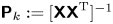 $\boldsymbol{\mathsf{P}}_k := [\boldsymbol{\mathsf{XX}}^\textrm {T} ]^{-1}$. If a new snapshot
 $(\boldsymbol {x}_{k+1}, \boldsymbol {y}_{k+1})$ is appended to the snapshot matrix, the estimate for
 $\boldsymbol{\mathsf{Q}}_k$ and
 $\boldsymbol{\mathsf{P}}_k$ can be updated as
 \begin{equation} \boldsymbol{\mathsf{Q}}_{k+1} = [\boldsymbol{\mathsf{Y}} \quad \boldsymbol{y}_{k+1}][\boldsymbol{\mathsf{X}} \quad \boldsymbol{x}_{k+1}]^\textrm{T} = \boldsymbol{\mathsf{Q}}_k + \boldsymbol{y}_{k+1} \boldsymbol{x}_{k+1}^\textrm{T} , \end{equation}
and
 \begin{equation} \boldsymbol{\mathsf{P}}_{k+1} = ([\boldsymbol{\mathsf{X}} \quad \boldsymbol{x}_{k+1}][\boldsymbol{\mathsf{X}} \quad \boldsymbol{x}_{k+1}]^\textrm{T})^{-1} = [\boldsymbol{\mathsf{P}}_k^{-1} + \boldsymbol{x}_{k+1} \boldsymbol{x}_{k+1}^\textrm{T} ]^{-1}. \end{equation}
The expression for  $\boldsymbol{\mathsf{P}}_{k+1}$ is now in a form that can be computed by the Sherman–Morrison formula,
 \begin{equation} \boldsymbol{\mathsf{P}}_{k+1} = [\boldsymbol{\mathsf{P}}_k^{-1} + \boldsymbol{x}_{k+1} \boldsymbol{x}_{k+1}^\textrm{T} ]^{-1} = \boldsymbol{\mathsf{P}}_k - \gamma \boldsymbol{\mathsf{P}}_k\boldsymbol{x}_{k+1}\boldsymbol{x}^\textrm{T}_{k+1}\boldsymbol{\mathsf{P}}_k . \end{equation}
The scalar  $\gamma$ is defined as
 $\gamma := 1/(1 + \boldsymbol {x}^\textrm {T}_{k+1}\boldsymbol{\mathsf{P}}_k\boldsymbol {x}_{k+1})$. Therefore, given current estimates of
 $\boldsymbol{\mathsf{Q}}_k$ and
 $\boldsymbol{\mathsf{P}}_k$, the DMD transition matrix is updated for each new snapshot by
 $\boldsymbol{\mathsf{A}}_{k+1} = \boldsymbol{\mathsf{Q}}_{k+1}\boldsymbol{\mathsf{P}}_{k+1}$. After some substitution (see Zhang et al. (Reference Zhang, Rowley, Deem and Cattafesta2019) for details),
 \begin{equation} \boldsymbol{\mathsf{A}}_{k+1} = \boldsymbol{\mathsf{A}}_k + \gamma(\boldsymbol{y}_{k+1} - \boldsymbol{\mathsf{A}}_k\boldsymbol{x}_{k+1})\boldsymbol{x}_{k+1}^\textrm{T}\boldsymbol{\mathsf{P}}_k . \end{equation}
As initial conditions,  $\boldsymbol{\mathsf{A}}_0$ can be initialized randomly, and
 $\boldsymbol{\mathsf{P}}_0 = \alpha \boldsymbol {I}$ such that the parameter
 $\alpha$ is very large yielding
 $\boldsymbol{\mathsf{P}}_0^{-1}\approx \boldsymbol {0}$ .
In order to discount the contribution of older snapshots on the current DMD estimate, a weighting factor  $\kappa$ is introduced to smoothly diminish their influence. The weighting factor acts on an ensemble of snapshot vectors as
 \begin{align} \boldsymbol{\chi} &= \begin{bmatrix} | & | & & | \\ (\sqrt{\kappa})^{\boldsymbol{n}-1} \boldsymbol{x}_1 & (\sqrt{\kappa})^{\boldsymbol{n}-2}\boldsymbol{x}_2 & \cdots & \boldsymbol{x}_{\boldsymbol{n}-1}\\ | & | & & | \end{bmatrix},\notag\\ \boldsymbol{\psi} &= \begin{bmatrix} | & | & & | \\ (\sqrt{\kappa})^{\boldsymbol{n}-1}\boldsymbol{x}_2 & (\sqrt{\kappa})^{\boldsymbol{n}-2}\boldsymbol{x}_3 & \cdots & \boldsymbol{x}_{\boldsymbol{n}}\\ | & | & & | \end{bmatrix}. \end{align}
The weighting factor is defined such that a desired half-life of  $\eta$ samples results in
 $\kappa = 2^{-1/\eta }$. Setting the weighting factor low (
 $\kappa \rightarrow 0$) aggressively attenuates old snapshots, while setting the weighting factor close to unity (
 $\kappa \rightarrow 1$) allows the old snapshots to gradually decay. These weighted snapshot matrices are substituted into the definition of DMD
 $\boldsymbol{\mathsf{A}}_W = \boldsymbol {\psi }\boldsymbol {\chi }^+$, and online DMD is carried out as before (Zhang et al. Reference Zhang, Rowley, Deem and Cattafesta2019). The end result is that the weighting factor adjusts the updated value of
 $\boldsymbol{\mathsf{P}}_{k+1}$ as
 \begin{equation} \boldsymbol{\mathsf{P}}_{k+1} =\frac{1}{\kappa} (\boldsymbol{\mathsf{P}}_k - \gamma \boldsymbol{\mathsf{P}}_k\boldsymbol{x}_{k+1}\boldsymbol{x}^\textrm{T}_{k+1}\boldsymbol{\mathsf{P}}_k). \end{equation}
This approach is useful for real-time DMD estimates as long as the computational effort required to update the DMD estimates remains low. Online DMD requires  $ \textit{O} (m^2)$ operations to update the DMD estimates (Zhang et al. Reference Zhang, Rowley, Deem and Cattafesta2019). Thus, this algorithm is well suited to the surface pressure array measurements with
 $m=13$ unsteady pressure sensors in the present case, in contrast to streaming DMD which are beneficial for high-dimensional data (Hemati, Williams & Rowley Reference Hemati, Williams and Rowley2014; Hemati et al. Reference Hemati, Rowley, Deem and Cattafesta2017). More information regarding the relative time required for various DMD algorithms is provided in Zhang et al. (Reference Zhang, Rowley, Deem and Cattafesta2019). It should be noted that this approach is formulated for cases in which there is no external forcing.
3.2. Including control inputs
DMD can be implemented for control cases by appending the DMD matrix as shown in Proctor et al. (Reference Proctor, Brunton and Kutz2016). For systems with no external inputs, current state observations are only a function of the previous state. However, this is not the case when forcing is introduced, and the natural state evolution should be separated from the influence of actuation. In this case, the linear discrete-time system provided by DMD should be of the form
 \begin{equation} \boldsymbol{x_{k+1}} = \boldsymbol{\mathsf{A}}_{DMD} \boldsymbol{x_{k}} + \boldsymbol{\mathsf{B}}_{DMD} \boldsymbol{u_{k}}, \end{equation}
when provided state measurements  $\boldsymbol {x_{k}}$ and prescribed input signals
 $\boldsymbol {u_{k}}$. This can be rewritten by appending the measurement matrix with the input array, resulting in
 \begin{equation} \boldsymbol{x_{k+1}} = \boldsymbol{\mathsf{A}}_{DMD} \boldsymbol{x_{k}} + \boldsymbol{\mathsf{B}}_{DMD} \boldsymbol{u_{k}} = \begin{bmatrix} \boldsymbol{\mathsf{A}}_{DMD} & \boldsymbol{\mathsf{B}}_{DMD} \end{bmatrix} \begin{bmatrix} \boldsymbol{x_{k}} \\ \boldsymbol{u_{k}} \end{bmatrix}. \end{equation}
This is rewritten in terms of the snapshot matrices as
 \begin{equation} \boldsymbol{\mathsf{Y}}= \boldsymbol{\mathsf{G}}_{DMD} \boldsymbol{{\Omega}}, \end{equation}
where  $\boldsymbol{\mathsf{G}}_{DMD}:= [\boldsymbol{\mathsf{A}}_{DMD} \ \boldsymbol{\mathsf{B}}_{DMD}]$ and
 $\boldsymbol {\Omega }:= [\boldsymbol{\mathsf{X}} \ \boldsymbol{\mathsf{U}}]^\textrm {T}$, in which
 $\boldsymbol{\mathsf{U}}$ is a matrix of the discrete input signals. This converts the problem back to the form of conventional DMD, thus the appended DMD matrix (
 $\boldsymbol{\mathsf{G}}_{DMD}$) is determined using an appropriate DMD algorithm (online DMD in this case). This process is referred to as DMD with control and more details are provided in Proctor et al. (Reference Proctor, Brunton and Kutz2016). Online DMD is then performed using the weighting factor to identify time-varying estimates of the linear transition matrix subject to actuation.
4. Closed-loop separation control approach
Since online DMD provides a linear representation of the evolution of the surface pressure fluctuations, classical linear control methods may be viable for autonomous feedback control. For example, if the objective is to suppress the pressure fluctuations, the control input can be defined as a state feedback  $\boldsymbol {u}_k = -\boldsymbol{\mathsf{K}}\boldsymbol {x}_k$, and the linear dynamics provided by online DMD can be expressed as
 \begin{equation} \boldsymbol{x}_{k+1} = (\boldsymbol{\mathsf{A}} - \boldsymbol{\mathsf{B}}\boldsymbol{\mathsf{K}})\boldsymbol{x}_k , \end{equation}
in which  $\boldsymbol{\mathsf{A}}$ is the current discrete linear state dynamics and
 $\boldsymbol{\mathsf{B}}$ is the current actuation mapping matrix identified by online DMD. At this point, the LQR method can be used to determine
 $\boldsymbol{\mathsf{K}}$ for the current system estimate with respect to a weighting term applied to the state and the actuator effort (Dorf & Bishop Reference Dorf and Bishop2011). As the flow is forced,
 $\boldsymbol{\mathsf{A}}$ will likely vary. Therefore, the
 $\boldsymbol{\mathsf{K}}$ matrix will need to be updated accordingly. In general, this feedback term will not provide optimal control since the underlying dynamics is time varying and nonlinear. However, this is the set of optimal feedback gains for the current dynamical estimate provided by online DMD.
Using the discrete linear system representation provided by online DMD, LQR controller feedback gains are computed and updated (not necessarily as frequently as the online DMD updates). These feedback gains are then employed to attenuate the unsteady pressure fluctuations within the separated flow region. The control signal is defined as a negative feedback
 \begin{equation} \boldsymbol{u}_k = -\boldsymbol{\mathsf{K}}_{LQR}\boldsymbol{x}_k . \end{equation}
In which,  $\boldsymbol{\mathsf{K}}_{LQR}$ is determined by minimizing the cost function
 \begin{equation} J =\sum_{k = 0}^{\infty} ( \boldsymbol{x}_k^\textrm{T} \boldsymbol{\mathsf{Q}}_{LQR} \boldsymbol{x}_k + \boldsymbol{u}_k^\textrm{T}\boldsymbol{\mathsf{R}}_{LQR} \boldsymbol{u}_k) . \end{equation}
See Dorf & Bishop (Reference Dorf and Bishop2011) for details. The choice of  $\boldsymbol{\mathsf{Q}}_{LQR}$ and
 $\boldsymbol{\mathsf{R}}_{LQR}$ selectively weights the performance and actuator input terms in (4.3). The solution for
 $\boldsymbol{\mathsf{K}}_{LQR}$ is
 \begin{equation} \boldsymbol{\mathsf{K}}_{LQR} = (\boldsymbol{\mathsf{R}}_{LQR} + \boldsymbol{\mathsf{B}}^\textrm{T} \boldsymbol{\mathsf{P}}_R \boldsymbol{\mathsf{B}})^{-1}\boldsymbol{\mathsf{B}}^\textrm{T}\boldsymbol{\mathsf{P}}_R\boldsymbol{\mathsf{A}} , \end{equation}
in which,  $\boldsymbol{\mathsf{P}}_R$ is determined from the discrete-time algebraic Riccati equation,
 \begin{equation} \boldsymbol{\mathsf{P}}_R = \boldsymbol{\mathsf{A}}^\textrm{T} \boldsymbol{\mathsf{P}}_R \boldsymbol{\mathsf{A}} -(\boldsymbol{\mathsf{A}}^\textrm{T} \boldsymbol{\mathsf{P}}_R \boldsymbol{\mathsf{B}})(\boldsymbol{\mathsf{B}}^\textrm{T} \boldsymbol{\mathsf{P}}_R \boldsymbol{\mathsf{B}} + \boldsymbol{\mathsf{R}}_{LQR})^{-1}(\boldsymbol{\mathsf{A}}^\textrm{T} \boldsymbol{\mathsf{P}}_R \boldsymbol{\mathsf{B}})^\textrm{T} + \boldsymbol{\mathsf{Q}}_{LQR} . \end{equation}
This process is implemented using the LabVIEW LQR VI from the control design and simulation module.
5. Analysis of the baseline separated flow
This section provides baseline separated flow characteristics including estimates of the spectral content of the flow from surface pressure measurements and full-field flow evaluation from TR-PIV measurements. The TR-PIV measurements allow for estimation of the unsteady pressure field determined via solution of Poisson's equation. These results are then compared to DMD analysis of the unsteady surface pressure measurements.
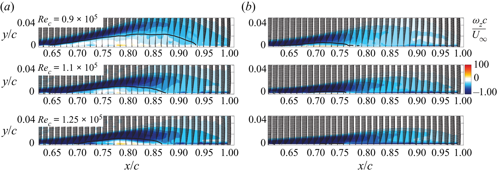
Figure 7 contains vorticity contours of the mean of PIV snapshots for the baseline separated flow. The separation region is illustrated by the line of  $\bar {u} = 0$, depicted as the black dashed line. The length of the mean separation bubble is
 $L_{sep} = 0.24 c$, and the height is
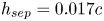 $h_{sep} = 0.017c$.
Average  $z$-vorticity as computed from PIV snapshots. The black line denotes the time-averaged
 $\bar {u} = 0$ contour. The red markers denote the probe locations from which data are extracted for the coherence estimates in figure 9.

5.1. Unsteady pressure
The unsteady pressure fluctuations within the separated flow are recorded by microphones that lie within the separated flow region and spectral content is estimated and plotted with respect to the Strouhal number, non-dimensionalized with respect to the separation bubble length and free-stream velocity,
 \begin{equation} St_{L_{sep}} = f L_{sep} / U_\infty, \end{equation}
where  $L_{sep}=0.24c$ for the baseline uncontrolled flow at
 $Re_c=10^5$.
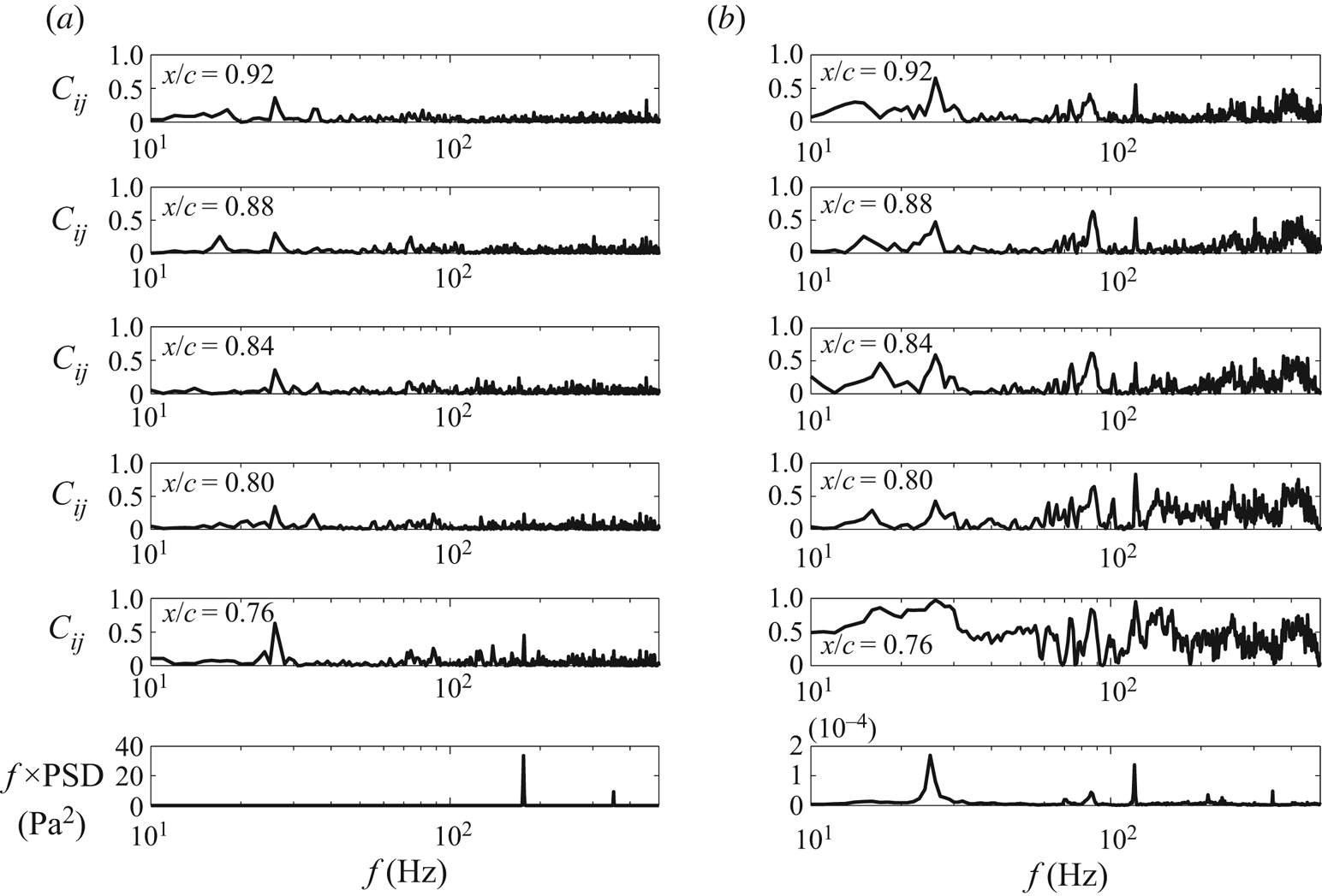
The coherence between each reference microphone and select surface mounted microphones is provided in figure 8. The premultiplied spectra are also provided for each reference microphone in figure 8. The reference microphones are mounted near the separation-duct fan and on the floor of the wind tunnel. High coherence is exhibited around 25 Hz (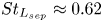 $St_{L_{sep}} \approx 0.62$) between the surface mounted microphones and the separation fan microphone. However, the spectrum of the separation fan microphone exhibits a dominant peak at 175 Hz, but very little power near 25 Hz. This is due to the fact that the separation fan consists of seven blades, so the peak at 175 Hz corresponds to the blade passage frequency of the fan, while 25 Hz is the rotation rate of the fan.
Coherence computed between select surface pressure microphones and the (a) separation fan reference microphone and (b) tunnel floor reference microphone. The microphone location for each plot is denoted at the top left of the plot. The last graph in each column provides the premultiplied power spectral density for each reference microphone.

Broadband coherence exists between the tunnel floor microphone and surface array microphones, with overall coherence decreasing as  $x/c$ increases. The primary coherence bands are around 25 Hz and within the frequency range of the flow. The power spectral density (PSD) of the tunnel floor reference microphone shows significant content at the rotation rate of the separation-duct fan (25 Hz). Additionally, a peak at 120 Hz exists due to line noise. Therefore, in order to remove the contamination due to the separation-duct fan pressure fluctuations at the rotation rate, a digital high pass filter is implemented with a cutoff frequency of 28 Hz. The signal attenuation of this filter at 25 Hz is
 $-$6.4 dB.
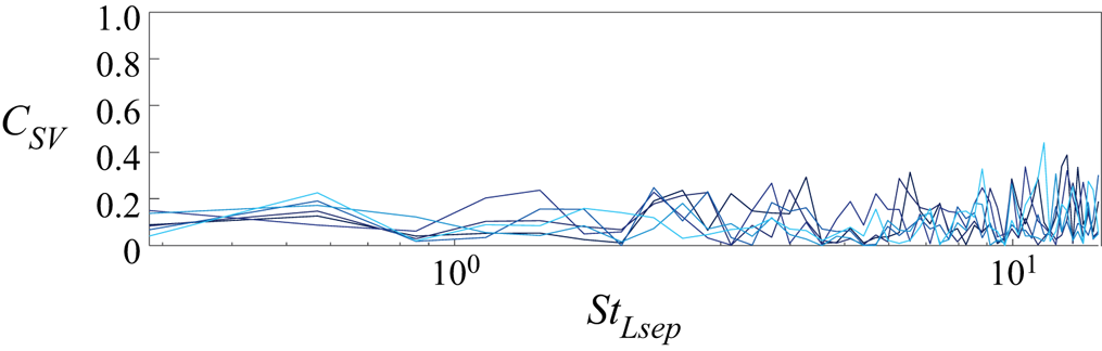
The non-negligible coherence between the unsteady pressure sensors and the separation fan rotation rate raises potential concerns regarding the flow's possible response to these small pressure disturbances. In order to evaluate whether the flow oscillations lock-on to the fluctuations from the separation-duct fan, the coherence between simultaneously sampled PIV velocity measurements and the separation-duct reference microphone measurements are computed. This is shown in figure 9 for several PIV vector locations within the separated flow region. No lock-on is observed as the coherence does not exceed 0.27 over the energetic frequency range of the separated flow. Therefore the flow is not significantly influenced by these extraneous disturbances.
Coherence between PIV  $v$-velocity measurements and unsteady pressure data from the separation-duct reference microphone for several points within the separated flow region. The probe locations are denoted by red markers in figure 7.

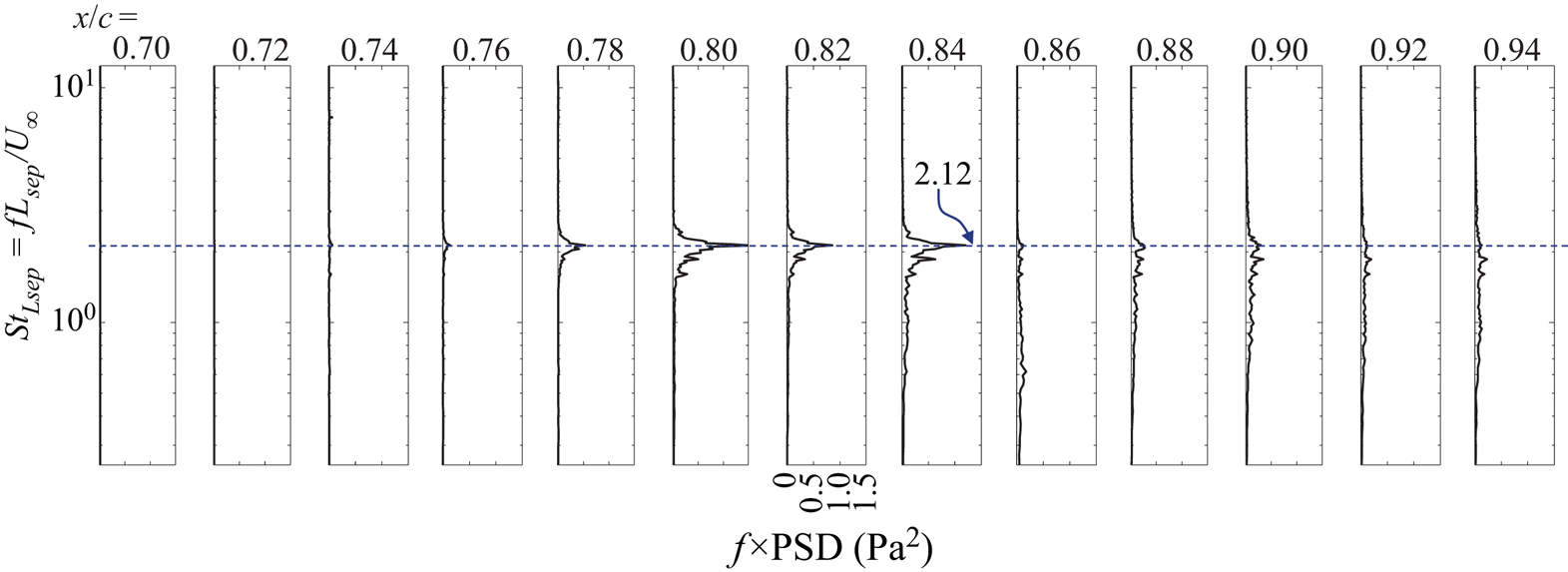
Premultiplied spectra for these measurements are plotted with respect to Strouhal number in figure 10 to show the streamwise development of the frequency content of the pressure fluctuations. For the plots shown, a total of 30 s of data acquired at 10 kHz are used to estimate the PSD. The number of samples used per block is 10 000 resulting in  ${\rm \Delta} f = 1$ Hz. A Hann window is used and the blocks are overlapped by 75 %, which results in a normalized random uncertainty of approximately 25 %. These plots show the streamwise growth of unsteady pressure content due to the Kelvin–Helmholtz instability vortex evolution in a frequency range between
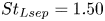 $St_{Lsep} = 1.50$ and 2.30. The dominant shear-layer frequency identified by the power spectrum is
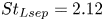 $St_{Lsep} = 2.12$. This content begins to decay before the mean reattachment region as the flow transitions to turbulent flow, and spectral broadening occurs.
Premultiplied PSD plots of the surface mounted microphone array measurements. The microphone location for each plot is denoted at the top of the plot.

5.2. Time-resolved PIV
PIV snapshots provide mean and turbulent quantities of the baseline flow field subject to spatial resolution limitations. Since a high speed PIV system is utilized, the sample rate of the velocity snapshots is much higher than the characteristic frequencies of the flow. Thus, dynamical information can be extracted from the flow field data by space–time POD, referred to here as simply POD, or by DMD. The TR-PIV datasets for the uncontrolled, canonical separated flow ( $Re_c=10^5$) studied here consist of
 $\boldsymbol {n}=10\ 000$ snapshots, each with
 $10\ 032$ 2-component vectors per snapshot such that
 $\boldsymbol {m}=20\ 064$ for the modal analysis.
5.3. Analysis of the baseline flow
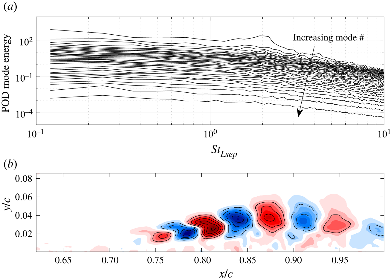
POD is applied to the TR-PIV snapshots of the baseline separated flow in order to identify global dynamical characteristics of the baseline flow. Using the ‘SPOD’ algorithm of Towne et al. (Reference Towne, Schmidt and Colonius2018) with  ${\rm \Delta} f=4.88$ Hz, a Hanning window, and 75 % overlap yields the modal energy spectrum in figure 11(a), with the arrow indicating increasing mode number. There is a broad peak in the spectrum at
 $St_{Lsep} \approx 2$ in the most energetic mode, and figure 11(b) shows the real part of the streamwise vorticity of this mode. This mode corresponds to large-scale vortical structures in the separated shear layer that convect downstream over the surface of the plate.
POD of baseline uncontrolled TR-PIV velocity field. (a) POD modal energy vs. Strouhal number and (b) real part of the dimensionless vorticity of the dominant POD mode at  $St \approx 2$. Dashed contour lines are shown for negative values and solid contour lines for positive values with an increment of 0.03.

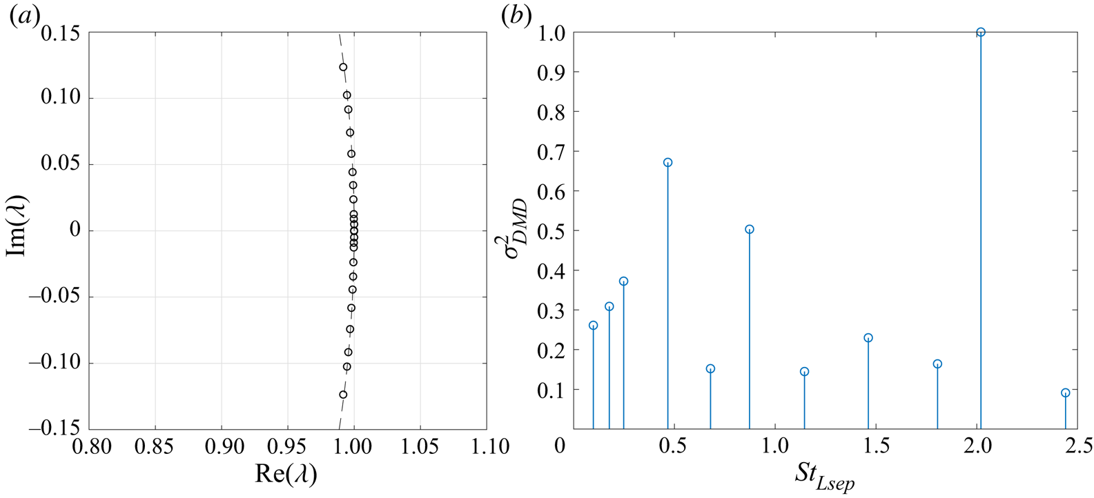
The broad peak in the POD spectrum is consistent with the peak in the power spectra from surface pressure measurements in figure 10. These results indicate the TDMD estimate can be rank reduced. A rank-reduction level of  $r = 25$ is used, which corresponds to retaining over 99 % of the fluctuating kinetic energy content. Figure 12 shows the DMD eigenvalues plotted in the complex plain along with the relative modal power plotted with respect to Strouhal number. The eigenvalue plot shows that the dominant modes extracted via TDMD are non-decaying and purely oscillatory (i.e. the eigenvalues lie very close to the unit circle). This is expected due to the oscillatory, stable limit cycle characteristics of the separated flow.
TDMD analysis of baseline uncontrolled TR-PIV velocity field with reduced rank of 25. (a) DMD eigenvalues obtained from TDMD plotted in the complex plain and (b) normalized spatial- and temporal-averaged modal power versus Strouhal number.

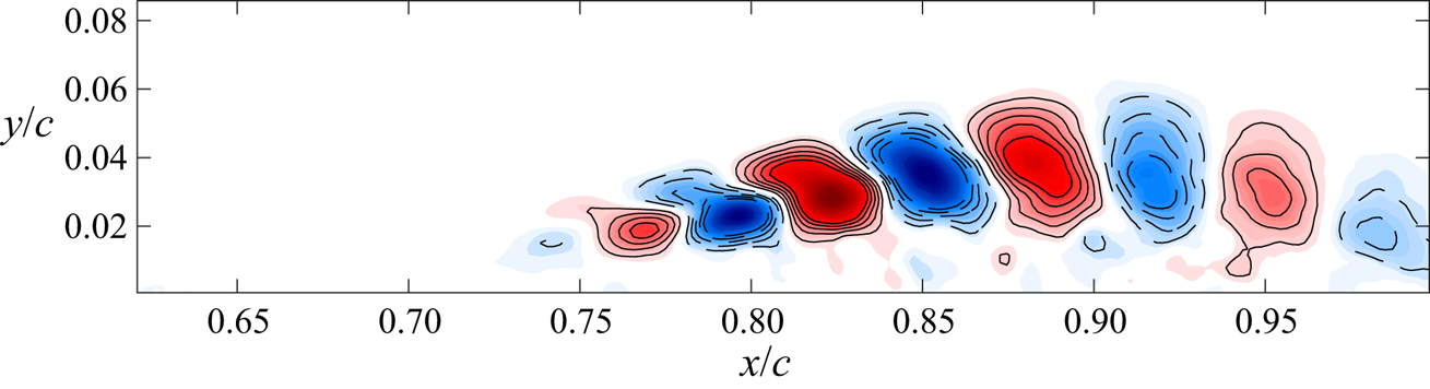
In addition, the highest modal power occurs at 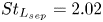 $St_{L_{sep}} = 2.02$, which agrees with the POD analysis. This TDMD mode describes the most energetic component of the shear-layer limit cycle of the baseline separated flow. In figure 13, the real part of the DMD mode is visualized as vorticity contours. This mode is analogous to the most energetic POD mode in figure 11(b) as expected. Experimentation with the rank reduction revealed no variation in the Strouhal number of the dominant mode or its spatial structure. Indeed, nearly identical results were obtained with
 $r$ as low as 10.
Real part of the dimensionless vorticity for the dominant TDMD mode at  $St \approx 2$ with a reduced rank of
 $r=25$. Same plot settings as in figure 11(b).

While performing TDMD on velocity field measurements by TR-PIV is valuable for examining the dynamics of the velocity field, such an analysis is not currently feasible in a real-time feedback control scheme. However, unsteady surface pressure measurements can be acquired and processed much more efficiently, thereby enabling real-time estimation of the separated flow dynamics. To this end, an estimate of the full pressure field is first computed from the velocity field TR-PIV measurements. Then, SP-TDMD will be applied to the pressure-field snapshots in order to systematically examine the trade-off between rank and the fidelity of the DMD approximation.
5.4. Pressure field via solution of Poisson's equation
In order to examine whether the dynamical characteristics of the separated flow are attainable from unsteady surface pressure measurements, the evolution of the pressure field is estimated by solving the pressure-Poisson equation, which is then evaluated with DMD. de Kat & Van Oudheusden (Reference de Kat and Van Oudheusden2011) demonstrate that time-resolved, planar PIV can be used to estimate the pressure-field snapshots of nominally two-dimensional flows. From the Navier–Stokes equations for momentum conservation in incompressible flows, the pressure gradient is determined by
 \begin{equation} \boldsymbol{\nabla} p= -\rho \left( \frac{\partial \boldsymbol{u}}{\partial t} + \left( \boldsymbol{u} \boldsymbol{\cdot} \boldsymbol{\nabla} \right) \boldsymbol{u} - \nu \nabla^2 \boldsymbol{u} \right).\end{equation}
Taking the divergence of (5.2) results in the pressure-Poisson equation, expressed using indicial notation as
 \begin{equation} \frac{\partial^2 p}{\partial x_i^2} = -\rho \left( \frac{\partial }{\partial x_i}\left( \frac{\partial u_i}{\partial t} \right) + \frac{\partial }{\partial x_i} \left( u_j\frac{\partial u_i}{\partial x_j} \right) -\nu \frac{\partial }{\partial x_i} \frac{\partial ^2u_i}{\partial x_j\partial x_j} \right) . \end{equation}
This is simplified by recognizing that the divergence of the velocity field is zero since the flow is incompressible. Therefore, the unsteady and viscous terms are zero. Since PIV measurements for the current study provide two-component planar velocity fields, the Laplacian of the pressure fluctuations is estimated assuming that there are no velocity components or gradients in the  $z$-direction
 \begin{equation} \nabla^2 p_{xy}= \frac{\partial^2p}{\partial {x}^2} + \frac{\partial^2p}{\partial {y}^2} = -\rho \left[ \left(\frac{\partial u}{\partial x}\right)^2 + 2\frac{\partial u}{\partial y} \frac{\partial v}{\partial x} + \left(\frac{\partial v}{\partial y}\right)^2 \right] .\end{equation}
Griffin (Reference Griffin2013) has shown this is a reasonable assumption for the time-averaged flow field using stereo-PIV in multiple spanwise measurement planes. To account for the reduced validity of this assumption within the regions of increased turbulence and three-dimensional mixing (de Kat & Van Oudheusden Reference de Kat and Van Oudheusden2011), the uncertainty of these estimates within the turbulent region is elevated.
Regarding sampling requirements for computing the pressure field from time-resolved PIV, de Kat & Van Oudheusden (Reference de Kat and Van Oudheusden2011) provided guidelines concerning the required spatial and temporal resolutions. In particular, the interrogation window size needs to be at least five times smaller than the flow structure of interest, while the sampling frequency needs to be at least an order of magnitude higher than the frequency of interest. Both of these conditions are satisfied for the large-scale vortical structures in the separated shear layer.
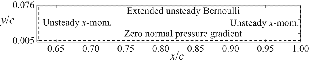
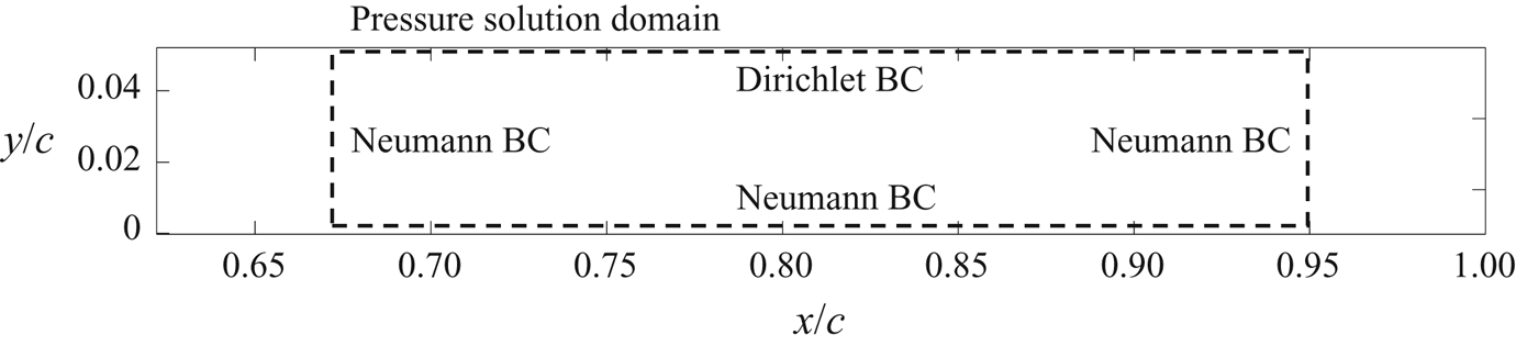
In solving for  $p_{xy}$, partial derivatives are estimated using a second-order, central difference scheme for interior points, and second-order, single-sided differences are computed for Neumann boundary conditions at the edges of the domain. Assuming that the upper boundary is outside the viscous and rotational regions of the flow but not quite in the free stream and also that the mean velocity gradients are small, an extended version of the unsteady Bernoulli equation is used as described by (9) in de Kat & Van Oudheusden (Reference de Kat and Van Oudheusden2011). As shown in figure 14, the lower boundary of the pressure computation region is slightly above the flat plate surface due to reflections. For this lower boundary, a zero pressure gradient is enforced in the vertical direction. The inlet and exit boundary conditions satisfy the unsteady
 $x$-momentum equation (
 $x$-component of (5.2)). The unsteady term in the momentum boundary condition is estimated via central differences between two neighbouring snapshots. The pressure computational grid is thus a subset of the PIV measurement domain that consists of
 $206 \times 43$ uniformly arranged points, the bounds of which are shown in figure 14.
Boundary conditions and domain for solution of the pressure-Poisson equation.

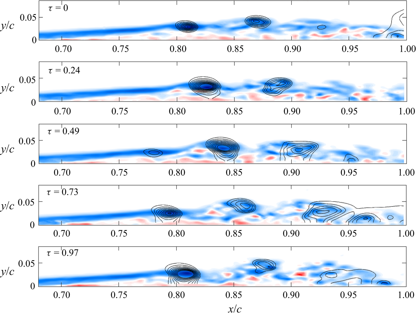
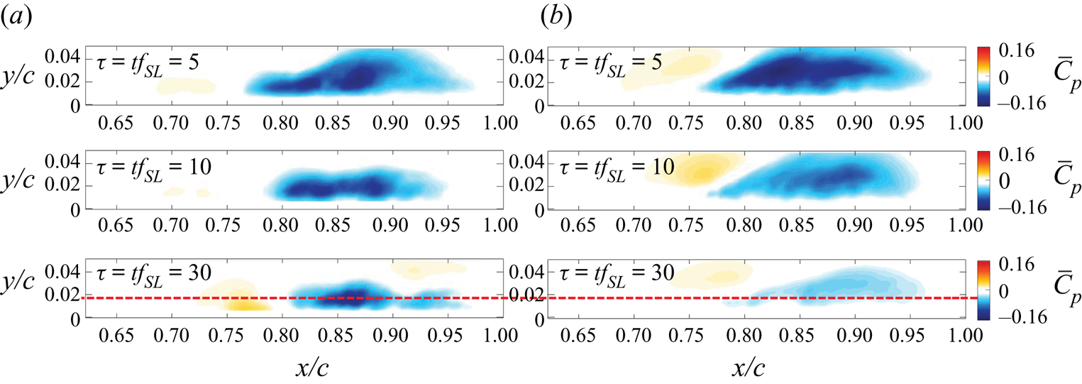
Sample results of this procedure are shown in figure 15, in which mean-subtracted pressure coefficient ( $C_{p'}$) contours are plotted with synchronized vorticity fields at different times, where
 $\tau = t/T_{SL}$ is time normalized by the period of the shear-layer dominant frequency at
 $St_{Lsep} = 2$, and
 $C_{p'}$ is defined here as
 \begin{equation} C_{p'} = \frac{p-\bar{p}}{\rho U_\infty^2/2}. \end{equation}
Snapshots of vorticity superimposed with mean-subtracted  $C_{p'}$ contours computed from the 2-D PIV vector field. Negative
 $C_{p'}$ contours are depicted with an increment of 0.05. Regions of low pressure convect with the vortices in the separated shear layer with an average velocity of
 $0.55U_{\infty }$.

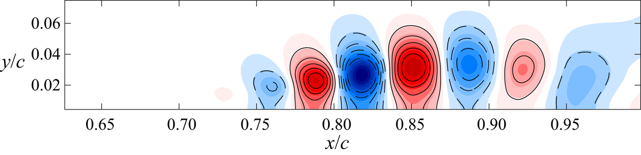
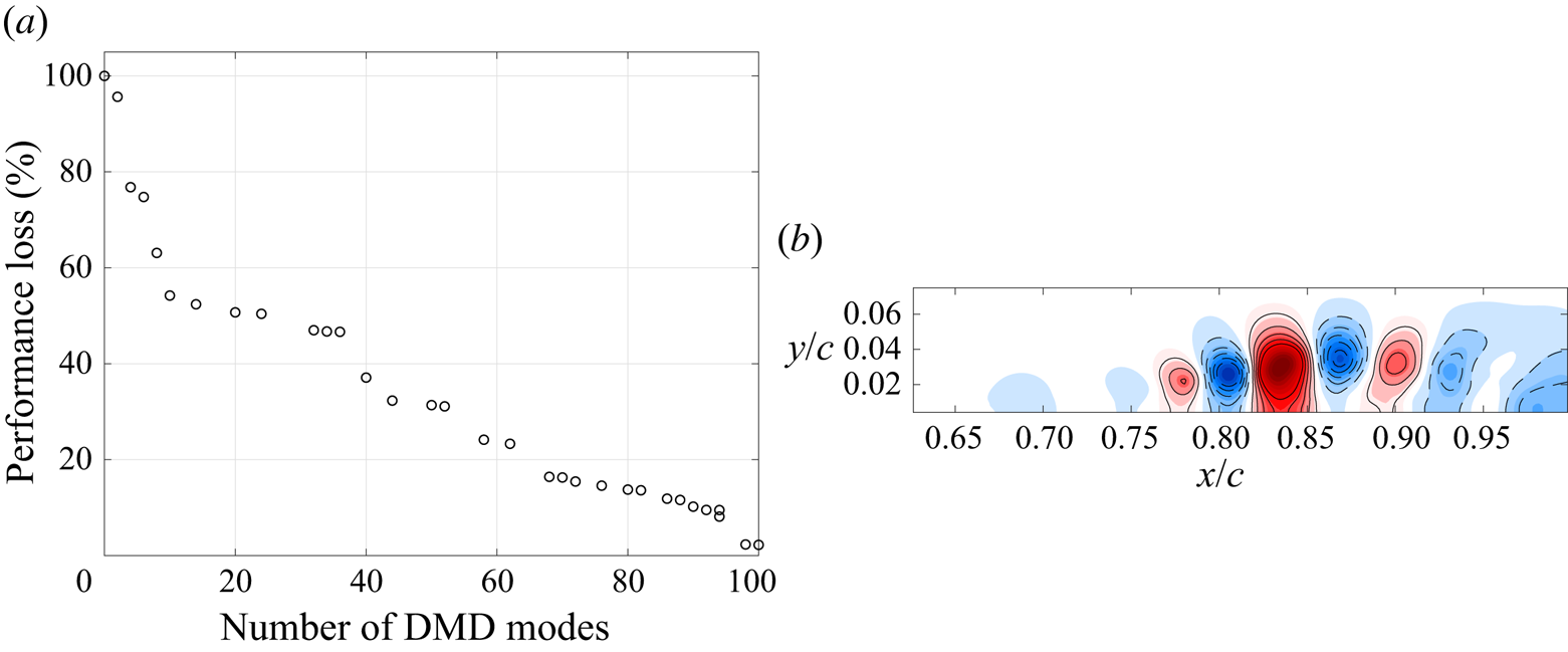
These plots show that low-pressure regions are located near the centres of the vortices in the separated shear layer. Applying POD to the pressure field snapshots reveals the quasi-periodic vortex train at  $St \approx 2$, as shown in figure 16. Therefore, it is expected that the convecting vortices will leave a traveling wave-like footprint on the surface of the plate. Since real-time POD is not currently feasible, we will resort below to online DMD, after using SP-TDMD of the pressure snapshots to assess how many modes (and, hence, how many pressure transducers) are required for a reasonable approximation. Figure 17 shows the results of using SP-TDMD on 300
 $C_{p'}$ snapshots, a duration which corresponds to
 $\approx 5$ cycles of the dominant POD mode at
 $St=2$. Defined in Jovanović et al. (Reference Jovanović, Schmid and Nichols2014), the ‘performance loss’ quantifies the accuracy of the approximation versus the number of modes used. With 100 modes, there is little loss of information, but the performance gradually degrades with fewer modes. Below 10 modes, there is a clear increase in performance loss above 50 %. Figure 17(b) shows a close resemblance of the DMD mode at
 $St=2.06$ to that of the POD analysis in figure 16.
Real part of the dominant POD mode at  $St \approx 2$ applied to
 $\boldsymbol {n}=10\ 000$ snapshots of the instantaneous
 $C_{p'}$ fields using the same settings as in figure 11(b).

Results of SP-TDMD on 300  $C_{p'}$ snapshots, which corresponds to five cycles of the dominant mode. (a) There is a clear degradation in performance using less than 10 modes. (b) Dashed and solid contour lines are shown for negative and positive values, respectively, using an increment of 0.025. (a) Performance loss and (b) real part of
 $C_{p'}$ TDMD mode at
 $St=2.06$.

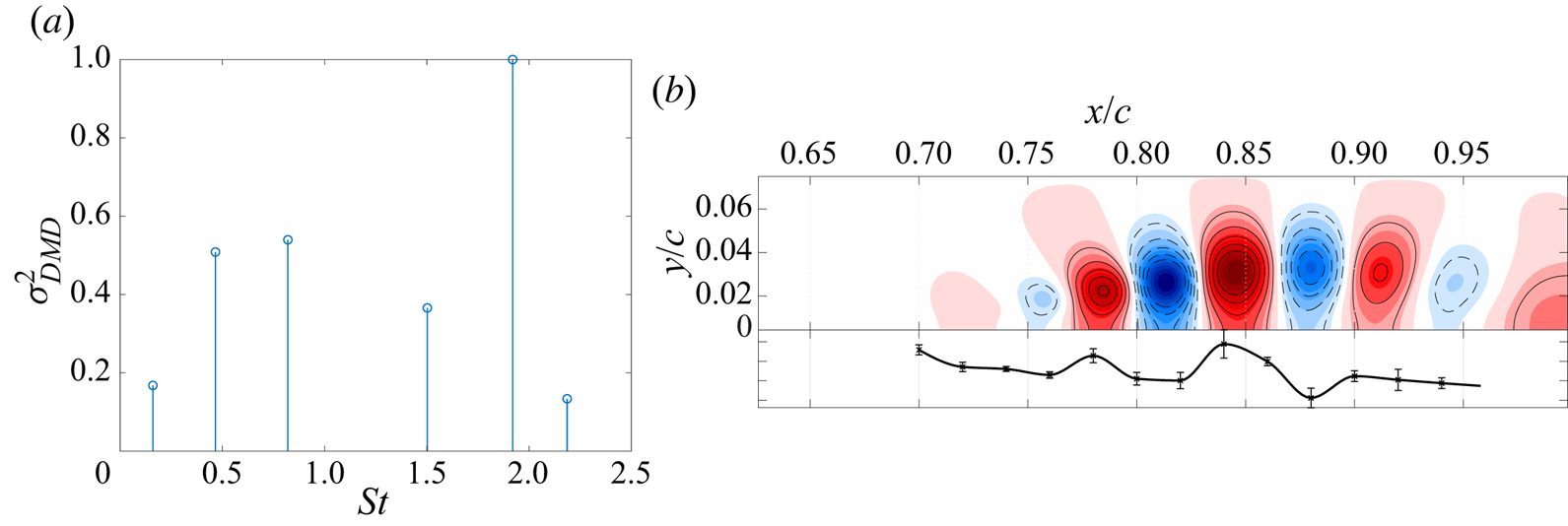
Figure 18 shows the result of TDMD analysis on all of  $C_{p'}$ snapshots using a reduced rank of
 $r=13$. The dominant mode has
 $St=1.92$, and panel (b) shows the real part of this dominant
 $C_{p'}$ DMD mode. Note the close similarity to the dominant POD mode in figure 16. Inspection of the spatial distribution of the mode reveals nearly vertical orientation of the structures, which implies that the separated flow modalities can indeed be obtained from measurements provided by the streamwise array of surface mounted microphones. The next section provides the results of analysing these measurements.
TDMD analysis of baseline uncontrolled  $C_{p'}$ field with reduced rank of 13. Same plot settings in (b) as in figure 17(b). (a) Normalized modal power and (b) real part of
 $C_{p'}$ TDMD mode at
 $St=1.92$ with the online DMD mode from the microphone array shown along the bottom for comparison.

5.5. Unsteady surface pressure DMD
Several studies have shown that effective separation control strategies are formed by exploiting the most amplified frequencies of the Kelvin–Helmholtz instability. Identifying dynamical characteristics of the separated flow (including the modality of the vortex generation due to the Kelvin–Helmholtz instability) in real time will enable feedback control of flow separation. The results of § 5.4 show that performing DMD on pressure-field snapshots yields similar dynamical characteristics to that of velocity. Also, § 5.1 shows that this dominant DMD mode frequency emerges as a peak in the power spectrum of the surface microphone array. Due to this correspondence, and the fact that these separated flow pressure modes likely leave a footprint on the surface of the model, a profile representation of the DMD modes should be obtained from the measurements of the surface pressure array microphones.
To confirm this, online DMD is performed on the simultaneously sampled surface pressure data with the retention factor set to  $\kappa = 0.99995$, such that 10 % snapshot attenuation occurs after
 $\tau = 35$ shear layer shedding periods. This allows for the DMD matrix to be updated with each new sample, while tracking temporal variations in the measured dynamics. In other words, a time-varying linear model of the nonlinear separated flow is provided in real time from surface pressure measurements.
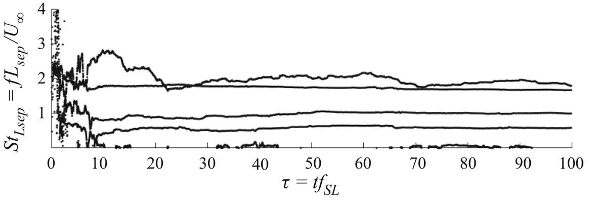
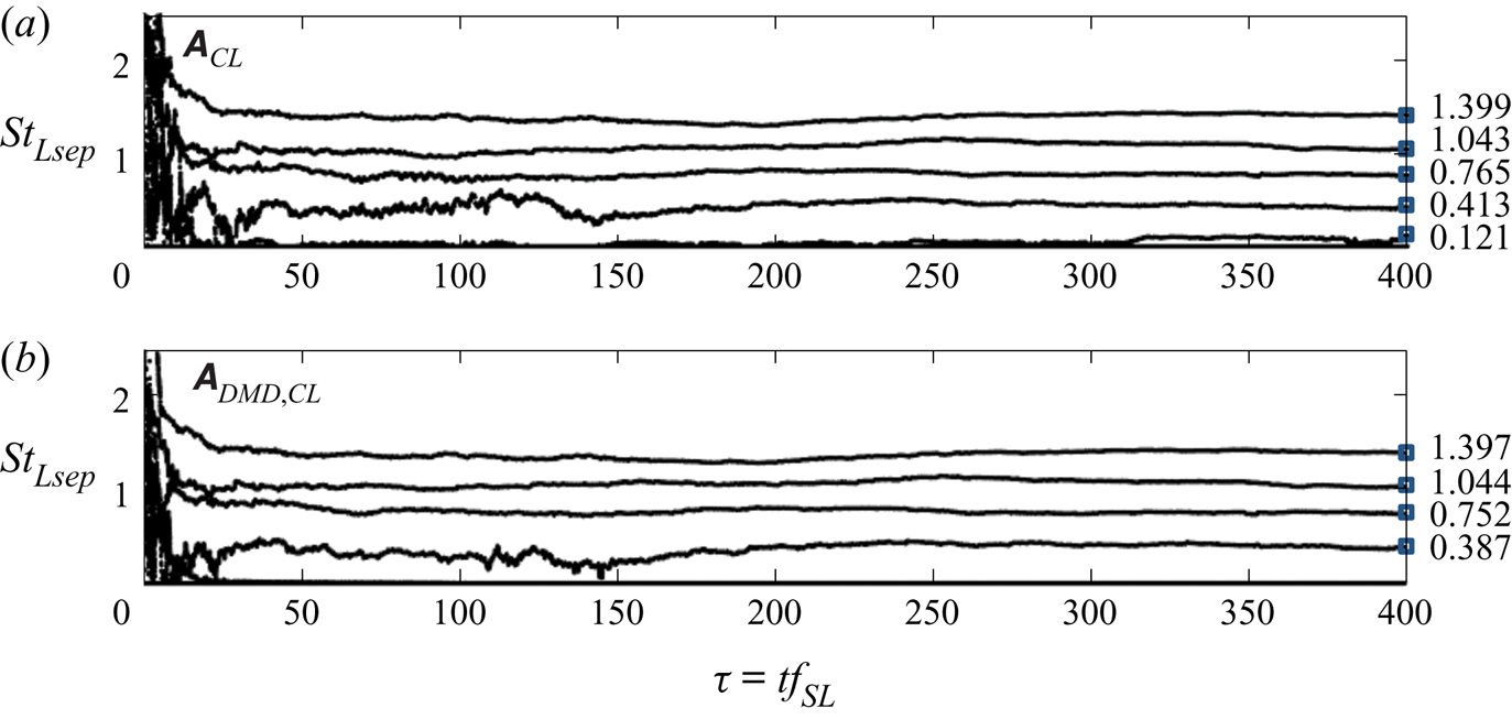
Since the surface pressure microphone array is comprised of 13 sensors, 13 eigenvalues will be available from the online DMD computation. This allows for a maximum of six distinct non-zero frequencies to be identified. Figure 19 shows the non-zero frequencies computed from the identified DMD eigenvalues via online DMD.
DMD frequencies identified by online DMD with a retention factor of  $\kappa = 0.99995$.

The online DMD algorithm begins with a random initial estimate of the dynamics, then the frequency estimates begin to settle after about  $\tau = 10$. The frequencies then appear approximately converged after
 $\tau = 30$. Four main frequencies exist, along with some low-frequency content. As with DMD of the flow field data, the dominant frequency at
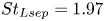 $St_{Lsep}=1.97$ due to the periodic shear-layer vortex generation is captured. After the start-up transient has decayed, the other identified DMD frequencies exhibit some wandering due to wind tunnel unsteadiness and measurement noise.
Since the DMD eigenvector estimates vary with each new sample provided to the online DMD algorithm, a statistical evaluation of the spatial modes is possible. The real part of the fluctuating surface pressure mode is plotted beneath the contour plot of the corresponding mode extracted from the Poisson solver in figure 18(b). The mode estimate corresponds to the online DMD output for  $\tau = 20$ to
 $80$, and the mean frequency is
 $St_{Lsep} = 1.97$. The variability of the mode shape is indicated via error bars with a length equal to the local standard deviation.
The dominant surface pressure DMD mode is clearly very similar to that estimated by PIV and the pressure-Poisson solution. Near  $x/c =0.8$, the wavelength of this mode is approximately
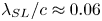 $\lambda _{SL}/c \approx 0.06$, which compares well to the shear-layer wavelength evaluated near the surface of the flat plate from the pressure-Poisson solution (
 $\lambda _{SL}/c \approx 0.058$). Since the temporal frequency and spatial wavelength of the wave packets that describe the evolution of the Kelvin–Helmholtz vortex convection are provided by DMD, the vortex propagation speed can be estimated from the two DMD estimates and the POD. This is the phase velocity, and is evaluated for the surface pressure online DMD results, the pressure-Poisson TDMD results, and the POD results as
 $v_p = \lambda \times f_{DMD} =$ 0.49, 0.46, 0.49, respectively. This agreement provides confidence in the online DMD method.
5.6. Transient characteristics of unforced reattachment
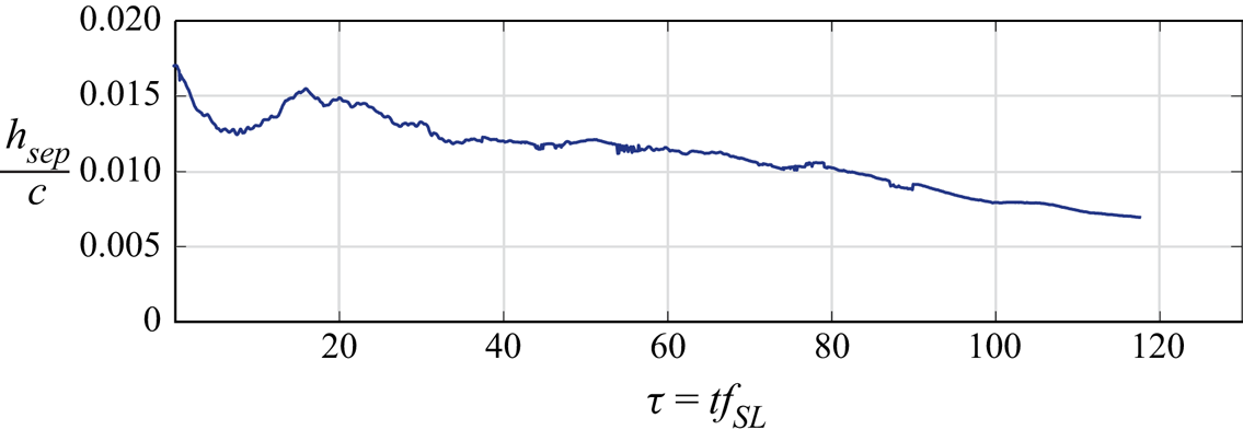
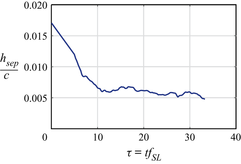
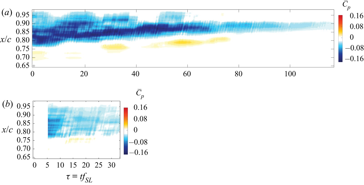
Before examining the impact of control, unforced reattachment is examined. In particular, by turning off the separation fan, the separated boundary layer gradually reattaches as the suction and blowing flow through the roof decay, and a nominally zero pressure gradient is re-established. The duration of this process will be compared to that of forced flow reattachment via active control. The mean separation height is computed via a moving average of the flow field comprised of 1250 snapshots at 10 kHz that is shifted by 10 snapshots recursively in time. This corresponds to an average of approximately 10 shear-layer periods, shifted by 0.08 periods. This allows for visualizing the evolution of the separation height as the flow reattaches once the separation system is turned off while attenuating high-frequency noise. The result is shown in figure 20, which indicates via linear extrapolation that the flow is fully reattached after approximately 200 time units.
Running calculation of the mean separation height to illustrate the transient response of the flow to turning off the separation system. Each moving mean calculation is comprised of 1250 PIV snapshots (approximately 10 shear-layer periods). (a) Unforced reattachment and (b) adaptive separation control.

6. Separated flow response to periodic forcing
The response of the separated flow subjected to periodic forcing is examined using PIV. Two momentum coefficients are tested for a range of actuation frequencies. The momentum coefficient is determined by computing the r.m.s. velocity as measured by PIV averaged across the actuator slot. The burst modulation waveform is used for these cases (see figure 21). As before, the nominal duty cycle of the modulation is set to 50 %, and the forcing frequency is defined as
 \begin{equation} F^+ = \frac{f_bL_{sep}}{U_\infty}. \end{equation}
Burst modulation waveform used for periodic actuation corresponding to 50 % duty cycle. In this case  $f_c = 2050$ Hz.

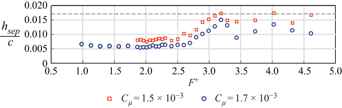
The forcing frequencies tested in this case span from  $F^+ = 0.98$ to 4.61, and the momentum coefficients tested are
 $C_\mu = 1.5\times 10^{-3}$ and
 $C_\mu = 1.7\times 10^{-3}$. For these momentum coefficient estimates, the 95 % confidence interval is 0.4 % of the momentum coefficient (Deem Reference Deem2018). As a comparative performance metric, the height of the mean reversed flow region is determined from PIV measurements for each forcing frequency (i.e. an indication for the size of the separation bubble) and plotted in figure 22. The random uncertainty in the estimated separation height is 0.5 % with 95 % confidence.
Normalized mean separation height plotted against input frequency. The minimum mean separation height measured corresponds to forcing near the dominant frequency identified by DMD,  $F^+ \approx 2$. The baseline separation height of
 $h_{sep}/c = 0.0171$ is denoted by the dashed grey line.

Flow separation is significantly reduced over a broad range ( $F^+ \approx 1$–2.5);
 $F^+ \approx 2$ corresponds to the dominant mode identified by POD and DMD. This corroborates the results of prior literature which show that targeting the shear-layer frequency of the separated flow is an effective strategy for reducing separation (Raju et al. Reference Raju, Mittal and Cattafesta2008; Griffin et al. Reference Griffin, Oyarzun, Cattafesta, Tu, Rowley and Mittal2013; Marxen et al. Reference Marxen, Kotapati, Mittal and Zaki2015; Hemati et al. Reference Hemati, Deem, Williams, Rowley and Cattafesta2016; Yarusevych & Kotsonis Reference Yarusevych and Kotsonis2017). Specifically, the greatest reattachment occurs for
 $C_{\mu } = 1.7 \times 10^{-3}$,
 $F^+ = 1.91$, with
 $h_{sep}/c = 0.0056$.
This illustrates that, for the goal of reducing the separation bubble height, the canonical separated flow is receptive to periodic forcing from a ZNMF jet actuator. Achieving this result in an autonomous manner for varying flow conditions is desired by utilizing this actuation approach with adaptive feedback control. The following section contains details regarding the implementation of such a controller and a discussion of its performance.
7. Adaptive control of separated flow
Online DMD is implemented at 10 kHz using the unsteady pressure within the separated flow region measured by the surface mounted, 13-element microphone array in order to estimate a linear model of the dynamical system responsible for the separated flow state evolution. This adaptive linear model is used in the control approaches described below. Each element of the control loop is coded in either Simulink or LabVIEW and compiled with NI Veristand 2017. The code is then deployed to an NI PXIe-8880 real-time controller for state measurement, online model estimation, feedback gain calculation and actuation signal generation.
Prior to being digitized, the microphone signals are low-pass filtered at a cutoff frequency of 500 Hz and ac coupled at 1 Hz by external variable frequency low-pass filters. This is accomplished with KEMO VFBF35 multi-channel filters and Stanford Research Systems SR640 low pass filters to attenuate the acoustic signal associated with the high frequency carrier sinusoid at 2050 Hz. The data acquisition rate is set to be 10 kHz for all control methods. For ZNMF actuation, the input waveform is multiplied by the carrier sine wave, amplified by a Trek PZD350 external amplifier, then sent to the actuator piezo-disks as a single-input signal.
7.1. Adaptive feedback control
An adaptive negative feedback controller is implemented by recursively computing LQR feedback gains for the current dynamical system estimate provided by online DMD (see § 4). For each primary control loop, the actuation input (4.2) is computed as the product of the LQR feedback gains with the surface pressure measurements.
As described in § 2.3, the ZNMF jet actuator operates by the modulation of a carrier frequency ( $\,f_c$). Therefore, the input value from the feedback controller is multiplied by the carrier sine wave before being provided to the actuator amplifier. Thus, the input waveform to the ZNMF jet takes on the form
 \begin{equation} V_{ZNMF,k} = u_k\times \sin(2{\rm \pi} f_c t_k) . \end{equation}
In this expression,  $u$ is the input computed from the feedback control loop and the subscript
 $k$ denotes iteration.
The nominal loop rate of the pressure snapshot acquisition, online DMD estimation, and input signal calculation is 10 kHz, which is more than 100 times faster than the dominant frequency of the separated flow. Due to the computational expense of solving the algebraic Riccati equation, the LQR feedback gains are updated every 40 primary loop cycles. This results in updating the feedback gains at a rate of 250 Hz. The online DMD weighting factor is set to  $\kappa = 0.99995$ in order to compromise between fast time response and attenuation of high-frequency noise. If time is non-dimensionalized with respect to the dominant DMD mode frequency (
 $\,f_{SL} \approx 81$ Hz), 10 % snapshot attenuation occurs after
 $\tau = 35$ characteristic periods.
The control performance is evaluated for varying values of the input penalty factor  $R_{LQR}$. Since only one independent actuator is employed,
 $R_{LQR}$ is a scalar, and is varied from
 $R_{LQR} = 0.1$ to
 $R_{LQR}=10$ while
 $\boldsymbol{\mathsf{Q}}_{LQR}$ is fixed at
 $20\boldsymbol {I}$. The mean separation height for each case is shown in figure 23(a). As
 $R_{LQR}$ is reduced, the penalty on actuator input is reduced, which results in increasing
 $C_\mu$ and smaller bubble heights. For
 $R_{LQR}$ values less than 1, the actuator gradually reaches its saturation limit. The value of the actuator momentum coefficient is plotted for the various values of
 $R_{LQR}$ in figure 23(b).
(a) Mean separation height and (b) actuator input as  $R_{LQR}$ is varied. The smallest bubble height occurs for
 $R_{LQR} = 0.2$. For
 $R_{LQR} < 1$, the separation height is
 $h_{sep}/c<0.006$. The baseline separation height of
 $h_{sep}/c = 0.0171$ and the lowest open-loop separation height of
 $h_{sep}/c = 0.0056$ are denoted by the dashed grey line. The momentum coefficient corresponding to this open-loop case is also provided (
 $C_\mu = 1.7\times 10^{-3}$).

Figure 24 shows a Pareto plot of mean separation bubble height versus momentum coefficient for both the open-loop and adaptive closed-loop control cases. This plot shows that the adaptive approach matches or exceeds the best performance of open-loop control. In addition, the trade-off between control performance and effort is clearly illustrated. Together, figures 23 and 24 enable a comparison between the open-loop and adaptive control cases. For example, an input penalty of  $R_{LQR} = 2$ results in
 $C_\mu = 1.3 \times 10^{-3}$ and
 $h_{sep}/c = 0.0059$, a bubble height that is only 5 % larger than the best-performing open-loop case that requires 30 % higher
 $C_\mu = 1.7 \times 10^{-3}$. These results indicate that the adaptive approach is beneficial because it reduces the extent of the separation more efficiently than open-loop control and achieves this in a rapid and autonomous manner.
Mean separation bubble height plotted versus momentum coefficient for both open-loop (OL) and adaptive closed-loop (CL) control.

Due to the unsteady nature of this adaptive control approach, the control input will vary as the separated flow deforms under actuation and the model is updated. Variations in the input signal are visualized as a spectrogram, shown for several cases in figure 25. Each input ensemble is scaled by a Hann window prior to computing the spectral estimates. The frequency resolution of the power spectrum is  ${\rm \Delta} f = 1$ Hz, the total length for each power spectral density estimate is 10 000 samples, and a new PSD is evaluated every 0.1 s (1000 samples). The time is non-dimensionalized with respect to the shear-layer frequency identified by DMD of the baseline flow. From the spectrogram, as soon as the control is turned on (
 $\tau = 0$), the input spectrum contains primarily low-frequency content for the cases shown (actuation effort is large). Then, the actuation signal exhibits a frequency between
 $St_{Lsep} =$1.5 and 1.8 for approximately 100 periods. After this, the actuation signal is primarily broadband, spanning frequencies up to
 $St_{Lsep} = 3$ for the most extreme cases. As expected, the total actuator power decreases as
 $R_{LQR}$ increases.
The frequency content of the actuation signal plotted with respect to shear-layer periods as a PSD spectrogram. This shows that the input signal exhibits time-varying and broadband frequency content and takes on multiple frequencies simultaneously.

Further attention will be given to the case in which  $R_{LQR} = 0.5$. The mean vorticity field computed from 4800 PIV snapshots is provided in figure 26. The recirculation region is significantly reduced, with a mean separation height of
 $h_{sep}/c = 0.0037$. The momentum coefficient is estimated from the PIV measurements for this case as
 $C_\mu = 2.5 \times 10^{-3}$.
Average  $z$-vorticity for separated flow subjected to adaptive LQR control as computed from 4800 PIV snapshots. The recirculation region is denoted by line of
 $\bar {u} = 0$ depicted by the solid black line. For reference, the recirculation region of the baseline separated flow is shown as the dashed orange line. For this case,
 $R_{LQR} = 0.5$. This shows that applying the adaptive feedback control using LQR gains significantly reduces the size of the separation region.

7.2. Moving mean and turbulence quantity evaluation
To visualize the transient response of the flow to LQR control, PIV acquisition is triggered by the initialization of the controller, and moving statistical quantities are computed from these data as in § 5.6. The moving mean separation height for the adaptive LQR control case in which  $R_{LQR}=0.5$ is shown in figure 27(a). From this plot, the mean separation height is significantly reduced after less than 10 characteristic periods. However, since the time window used in the estimation of the moving mean is also
 $\sim$10 periods, it is reasonable to expect that reattachment occurs earlier than
 $\tau = 10$, since this is the mean of the flow from
 $\tau = 5$ to
 $\tau = 15$. This reattachment is much quicker than the unforced reattachment from § 5.6.
Running calculation of the mean separation height to illustrate the transient response of the flow to adaptive LQR control for  $R_{lqr}=0.5$. This is computed from estimating the mean within a time window of
 $\tau = 10$ characteristic periods (ensembles of 1250 PIV snapshots).

The moving turbulence quantities ( $\overline {u'u'}$,
 $\overline {v'v'}$, and
 $\overline {u'v'}$ ) are plotted in figure 28 for several instances for both the unforced reattachment and the adaptive separation control. After 10 periods, the variance in the streamwise velocity is increased for the adaptive control case, while the unforced reattachment exhibits gradual reduction in all fluctuating quantities. However, by 30 periods, the overall levels of turbulent fluctuations are reduced compared to that of the unforced reattachment. This behaviour suggests that the adaptive control accelerates the occurrence of turbulent transition, which allows for enhanced mixing with the free-stream flow, re-energizing the boundary layer and reattaching the flow. In contrast, the unforced reattachment gradually evolves to a fully attached, laminar boundary layer.
Running calculation of the Reynolds stress components illustrate the evolution of the turbulent stresses subject to unforced reattachment vs. adaptive control ( $R_{LQR}=0.5$). This is computed over a time window of
 $\tau = 10$ characteristic periods (ensembles of 1250 PIV snapshots). (a) Unforced reattachment and (b) adaptive separation control.

7.2.1. Removing control
To evaluate the transient characteristics exhibited when control is removed and the flow is allowed to return to the baseline separated flow conditions, PIV measurements are triggered to acquire snapshots the moment control is disabled. From these measurements, the running mean separation height is calculated as before. As shown in figure 29, the separation bubble height first overshoots its baseline value at 10 time units and oscillates before settling down after approximately 50 time units. This is slower and more oscillatory in comparison with the establishment of control shown in figure 27 and is consistent with other studies that indicate that the overall time scale for separation can be several times larger than that of reattachment (Amitay & Glezer Reference Amitay and Glezer2006; Siauw et al. Reference Siauw, Bonnet, Tensi, Cordier, Noack and Cattafesta2010).
Running calculation of the mean separation height to illustrate the transient response of the flow when adaptive control turned off. The moving mean is estimated over a time window of  $\tau = 10$ characteristic periods (1250 PIV snapshots).

7.3. Moving mean pressure-field evaluation
Since a primary detriment of flow separation is the increased pressure drag, the effect of control on a moving mean calculation of the pressure field is evaluated. This is accomplished by estimating the pressure field from the mean pressure-gradient term in the Reynolds-decomposed Navier–Stokes equations as in van Oudheusden et al. (Reference van Oudheusden, Scarano, Roosenboom, Casimiri and Souverein2007). From the Reynolds-averaged Navier–Stokes equation, the gradient of the mean pressure field is
 \begin{equation} \frac{\partial \bar{p}}{\partial x_i} = -\rho \left( \frac{\partial {\overline{ u_i}}}{\partial t} + \overline{u_j} \frac{\partial \overline{u_i}}{\partial x_j} + \frac{\partial ( \overline{u_i'u_j'})}{\partial x_j} - \nu \frac{\partial }{\partial x_j}\frac{\partial \overline{u_i} }{\partial x_j} \right) . \end{equation}
Taking the divergence of this equation yields the mean pressure-Poisson equation.
 \begin{equation} \frac{\partial }{\partial x_i} \frac{\partial \bar{p}}{\partial x_i} = -\rho \left( \frac{\partial }{\partial x_i} \frac{\partial {\overline{ u_i}}}{\partial t} + \frac{\partial }{\partial x_i} \left( \overline{u_j} \frac{\partial \overline{u_i}}{\partial x_j} \right) + \frac{\partial }{\partial x_i} \frac{\partial ( \overline{u_i'u_j'} )}{\partial x_j} - \nu \frac{\partial }{\partial x_i}\left( \frac{\partial }{\partial x_j}\frac{\partial \overline{u_i} }{\partial x_j} \right) \right) . \end{equation}
This is simplified by removing the entries that are zero by continuity
 \begin{equation} \frac{\partial }{\partial x_i} \frac{\partial \bar{p}}{\partial x_i} = -\rho \left( \frac{\partial \overline{u_i}}{\partial x_j} \frac{\partial \overline{u_j} }{\partial x_i} + \frac{\partial^2 \overline{u_i'u_j'}}{\partial x_i \partial x_j} \right) . \end{equation}
The terms on the right-hand side of this equation are computed from the PIV measurements, for running ensembles of 1250 snapshots. The moving mean pressure field is then solved for every 10 snapshots. For the interior points, a central difference scheme estimates the Laplacian. For the boundaries of the domain, one-sided differences are computed with Neumann boundary conditions enforced for the left (inlet), right (outlet) and wall boundaries. Specifically, the streamwise mean pressure gradient as defined by (7.2) is enforced for the inlet and outlet. At the wall, zero vertical pressure gradient is enforced. Since this is a solution of the mean pressure field, a Dirichlet condition is enforced along the entire top boundary such that the mean pressure is defined by Bernoulli's equation, assuming that this region has negligible viscous contribution. This is in contrast to the boundary condition enforced for the instantaneous pressure-field calculation described earlier. The bounds of the pressure-field computational domain are illustrated in figure 30.
Bounds of the region in which the moving mean pressure field is solved for by the pressure-Poisson equation.

The results of these computations are provided in figure 31 for several instances. Rapid pressure recovery is shown for the adaptive separation control case ( $R_{LQR}=0.5$) such that, by 30 periods, the low pressure is increased by approximately 70 % compared to that for the unforced reattachment. In order to better visualize the evolution of the pressure field, a profile of the moving mean pressure field is extracted for each successive mean pressure calculation at
 $y/c \approx 0.019$. The location of this profile is depicted by the red dashed line in figure 31. Each extracted profile is arranged and plotted with respect to time. This provides a contour map of the pressure profile as it evolves with time. See figure 32 for the plots of the pressure profiles for the unforced reattachment and adaptive control respectively. As is indicated in figure 32(b), the pressure recovers very rapidly for the adaptive control, requiring only 10 periods for a significant reduction in low-pressure extent. In contrast, a much more gradual recovery is exhibited for the unforced reattachment.
Moving calculation of the mean pressure field. This is computed from moving time window of  $\tau = 10$ characteristic periods (ensembles of 1250 PIV snapshots). The red dashed line depicts the location of the pressure profile extracted for figure 32. (a) Unforced reattachment and (b) adaptive separation control.

Evolution of moving mean pressure profile at  $y/c \approx 0.019$ for the (a) unforced reattachment case and (b) adaptive separation control case (
 $R_{LQR}=0.5$). The
 $x$-axes for these plots are aligned.

7.4. Offline model identification
To illustrate the benefit of allowing the dynamical model to adapt as actuation is applied, closed-loop control is implemented for a dynamical model that is identified offline, from previously acquired data of the separated flow subject to open-loop control. In this case, the actuation condition used to develop the dynamical model corresponds to burst modulation forcing in which  $C_\mu = 1.7 \times 10^{-3}$ and
 $F^+ = 1.91$. This is the actuation signal that results in the largest reduction in separation height for all open-loop forcing cases studied. Here, 10 s of surface pressure measurements are processed by online dynamic mode decomposition with control (DMDC) with a weighting factor of 1 to provide a single offline estimate of
 $\boldsymbol{\mathsf{A}}_{DMD}$ and
 $\boldsymbol{\mathsf{B}}_{DMD}$. Then, LQR gains are computed for the identified dynamical system, which are then utilized for feedback control. For this case,
 $\boldsymbol{\mathsf{Q}}_{LQR} = 20\boldsymbol {I}$ and
 $R_{LQR} = 0.5$.
The mean vorticity for the non-adaptive control case is shown in figure 33. This result indicates that the separation region is shifted upstream slightly compared to the baseline separation. However, this control approach is largely ineffective since the height and extent of the separation region is essentially unchanged. This can be attributed to the fact that, for online DMD to estimate the actuation mapping  $\boldsymbol{\mathsf{B}}_{DMD}$, the response to actuator input must be observed. And, in this case, this open-loop actuation results in the largest deviation from the baseline dynamics of all the open-loop tests. Therefore, the actuation receptivity is likely significantly different for this deformed flow field, than for the natural separated flow dynamics. Thus, adaptive models ensure that the dynamical estimates and actuation mapping are current and accurate.
Average  $z$-vorticity for separated flow subjected to LQR control in which the model is determined offline. The recirculation region is denoted by the line of
 $\bar {u} = 0$ depicted by the solid black line. For reference, the recirculation region of the baseline separated flow is shown as the dashed orange line. This shows that the offline model identification is not an appropriate approach for reducing the separation region.

8. Evaluation of closed-loop dynamic modes
Online DMD estimates the plant dynamics  $\boldsymbol{\mathsf{A}}_{DMD}$ and
 $\boldsymbol{\mathsf{B}}_{DMD}$ that best describe the evolution of the surface pressure measurements in a linear sense as in
 \begin{equation} \boldsymbol{x}_{k+1} \approx \boldsymbol{\mathsf{A}}_{DMD} \boldsymbol{x}_{k} + \boldsymbol{\mathsf{B}}_{DMD} \boldsymbol{u}_{k} . \end{equation}
For the case in which feedback control is applied by gains identified by an LQR approach, the next surface pressure snapshot can be approximated by
 \begin{equation} \boldsymbol{x}_{k+1} \approx ( \boldsymbol{\mathsf{A}}_{DMD} - \boldsymbol{\mathsf{B}}_{DMD}\boldsymbol{\mathsf{K}}_{LQR} ) \boldsymbol{x}_{k} . \end{equation}
The terms in the parentheses can be combined and describe the closed-loop dynamics
 \begin{equation} \boldsymbol{\mathsf{A}}_{CL} = \boldsymbol{\mathsf{A}}_{DMD} - \boldsymbol{\mathsf{B}}_{DMD}\boldsymbol{\mathsf{K}}_{LQR} , \end{equation}
such that  $\boldsymbol {x}_{k+1} \approx \boldsymbol{\mathsf{A}}_{CL} \boldsymbol {x}_{k}$. A plot of these closed-loop frequency estimates is provided in figure 34(a). Once control is established, the primary dynamically relevant frequency reduces from approximately
 $St_{Lsep} = 2$ to
 $St_{Lsep} = 1.4$. The precise physical reason for this change is unclear, but may be due in part to an observed
 $\approx$23 % increase in momentum thickness just upstream of separation (Morris & Foss Reference Morris and Foss2003).
Frequencies of the closed-loop eigenvalues determined (a) by online DMD with control by computing  $\boldsymbol{\mathsf{A}}_{CL} = \boldsymbol{\mathsf{A}}_{DMD} - \boldsymbol{\mathsf{B}}_{DMD}\boldsymbol{\mathsf{K}}_{LQR}$ and (b) by direct estimation of the closed-loop dynamics by online DMD (
 $\boldsymbol{\mathsf{A}}_{DMD,CL}$). The frequency estimates for
 $\tau = 400$ are provided for each plot for comparison.

To validate the estimate of the control matrix  $\boldsymbol{\mathsf{B}}_{DMD}$ provided by online DMD with control, online DMD can be employed to estimate the closed-loop dynamics directly by neglecting the input term
 $\boldsymbol {u}_k$ and focusing only on the snapshot evolution as in (3.1). This dynamical system estimate will be referred to as
 $\boldsymbol{\mathsf{A}}_{DMD,CL}$. In this manner, online DMD should identify a matrix that is equivalent to the closed-loop mapping from (8.3), such that
 $\boldsymbol {x}_{k+1} \approx \boldsymbol{\mathsf{A}}_{DMD,CL} \boldsymbol {x}_{k}$. Any differences between
 $\boldsymbol{\mathsf{A}}_{DMD,CL}$ and
 $\boldsymbol{\mathsf{A}}_{CL}$ can be attributed to errors incurred by estimating the response to actuation by
 $\boldsymbol{\mathsf{B}}_{DMD}$.
To begin comparing the differences in the characteristics from both closed-loop estimates, the DMD frequencies computed from the closed-loop eigenvalues are evaluated. The temporal evolution of these frequencies are provided in figure 34 for the closed-loop dynamics directly estimated by online DMD ( $\boldsymbol{\mathsf{A}}_{DMD,CL}$) and by computing
 $\boldsymbol{\mathsf{A}}_{CL}$ from (8.3). For both estimation methods, the primary frequency is notably lower than that of the baseline dynamics. This characteristic was also seen in the stability results of Marxen et al. (Reference Marxen, Kotapati, Mittal and Zaki2015) and Yarusevych & Kotsonis (Reference Yarusevych and Kotsonis2017). Also, both methods exhibit similar variations for the lowest frequency up until roughly 150 periods. However, the extent of the variation differs somewhat between the different estimation methods. Overall, the characteristic frequencies identified between directly estimating the closed-loop dynamics and computing
 $\boldsymbol{\mathsf{A}}_{CL}$ show good agreement, with only subtle differences, most notably with respect to the near zero-frequency eigenvalue for
 $\boldsymbol{\mathsf{A}}_{CL}$.
9. Varying Reynolds number
To assess the robustness of this adaptive control approach, the chord Reynolds number is varied, and control is applied using the same parameters as before. Three additional Reynolds numbers are investigated by altering the free-stream velocity:  $Re_c = 0.9 \times 10^5, 1.1 \times 10^5,$ and
 $1.25 \times 10^5$. The separated flow is induced in the same manner as before, with the separation fan conditions fixed for all cases. Thus, the separation bubble characteristics vary due to the altered free-stream velocity. As the free-stream velocity increases, the extent of the baseline mean separation bubble is reduced since the higher momentum flow inhibits separation for the same setting of the ceiling fan. This is depicted in the flow fields provided in figure 35(a). The change in mean flow structure results in differing dynamical characteristics. The dimensional shear-layer frequency tends to increase with increasing Reynolds number. The dimensional frequency for each shear-layer mode is
 $f_{SL} = 70, 95$ and 105 Hz, and the separation length is
 $L_{sep}/c = 0.31, 0.23$ and 0.18, for
 $Re_c = 0.9 \times 10^5, 1.1 \times 10^5,$ and
 $1.25 \times 10^5$, respectively.
Time-averaged  $z$-vorticity for separated flow subjected to adaptive LQR control computed from 4800 PIV snapshots. The mean recirculation region is denoted by a solid black line corresponding to
 $\bar {u} = 0$. This shows that applying the adaptive feedback control using LQR gains significantly reduces the size of the separation region. (a) Baseline and (b) controlled.

The response of each flow to adaptive separation control is provided as mean vorticity fields in figure 35(b). For each case, the mean recirculation region is significantly reduced by the adaptive control approach. The input penalty is to  $R_{LQR} = 0.5$ for all three cases. The transient response to the control method is provided as a running mean calculation of separation height in figure 36. As with the original case, approximately 10 characteristic periods are required before the separation is significantly reduced.
Running calculation of the mean separation height to illustrate the transient response of the flow to adaptive separation control for varying Reynolds numbers. This is computed from the mean of a time window of  $\tau = 10$ characteristic periods (ensembles of 1250 PIV snapshots).

10. Conclusions
Real-time adaptive control is implemented to reattach separated flow in an autonomous manner. Measurements of unsteady surface pressure are used to determine a linear model of the flow that is allowed to update with each new measurement. This allows the estimate of the dynamical system to update in real time as forcing is applied and new flow modes are excited or nonlinear deviations occur. This adaptive dynamical estimate enables the use of linear closed-loop control techniques to efficiently reattach the separated flow.
To provide a repeatable separated flow that is not dependent upon specific airfoil curvature, separation is induced over a flat plate model in which the chord Reynolds number of the primary experiments is  $10^5$ and
 $Re_{\delta }\approx 920$ upstream of separation (
 $x/c \approx 0.3$). The flow is forced by a 2-D ZNMF jet in which the output is monitored by PIV both near the jet exit, and within the separated flow region. By measuring the response of the flow to periodic forcing, the most effective control is achieved when the modulation frequency is near that of the frequency of the shear-layer DMD mode.
Adaptive feedback control is then implemented in which LQR gains are recursively computed as the model estimates change. Since this is not a linear time invariant system, this is not optimal control per se, though it does provide the optimal control gains for the current linear time invariant system estimate. PIV measurements show that the mean separation region for this control case is significantly reduced. Comparing the efficiency of the adaptive control approach to open-loop control indicates that approximately 30 % less actuation effort is required for a comparable reduction in the separation bubble height. Furthermore, due to the quickly adapting model and feedback gain calculation, this control approach allows for rapid flow reattachment. Less than ten characteristic time units are required for the flow to reattach. Analysis of the temporal variation of the power spectral content of the actuator signal indicates that the model adaptation results in altered input characteristics as actuation is applied. Initially, the control input exhibits primarily low-frequency content, and eventually settles at a frequency that is somewhat lower than the baseline shear layer frequency. At a later stage, the actuation takes on a wider frequency range. This indicates that, once the separation region has been reduced, broadband actuation is required to retain the low separation region of the controlled flow.
By visualizing the estimation of the Reynolds stresses as the flow changes due to forcing, the control approach stimulates the early destabilization of the coherent shear-layer vortices, leading to earlier turbulent transition. This allows for more efficient mixing with the high-momentum free-stream flow, re-energizing the boundary layer to facilitate reattachment. Moving calculations of the mean pressure field are provided to show the extent and rate at which pressure recovery occurs under adaptive control.
The deformation of the dynamics as forcing is applied is a primary motivator for the use of adaptive control for reducing flow separation. This deformation is depicted by the variation in the dynamic modes and eigenvalues of the flow. Analysis of the time-varying eigenvalue estimates indicates that the frequency of the primary DMD mode decreases as forcing is applied. This corroborates the results of Marxen et al. (Reference Marxen, Kotapati, Mittal and Zaki2015) and Yarusevych & Kotsonis (Reference Yarusevych and Kotsonis2017).
Since this approach does not require any prior information regarding the dynamical characteristics of the flow, this approach is robust to varying flow conditions. Within the constraints of the experimental apparatus, the Reynolds number was varied from  $Re_c = 0.9\times 10^5$ to
 $Re_c = 1.25 \times 10^5$, and the adaptive control was applied to test robustness to varying flow conditions. By altering the Reynolds number, the separation bubble height and characteristic frequencies were varied. For all cases, the separation bubble height was either significantly reduced or eliminated, thereby reducing the losses incurred by boundary layer separation. Furthermore, no more than 10 characteristic periods were required to significantly reduce the mean separation region.
Additional investigations beyond the scope of this work should include analysis of the performance of this adaptive control approach to further separated flow conditions and characteristics. Pertinent examples of this may include an open separation that does not exhibit mean reattachment, which is analogous to leading-edge stall on an aerofoil, and a separation of fully turbulent boundary layer.
Acknowledgements
Funding for this work is provided under AFOSR grants FA9550-14-1-0289, FA9550-17-1-0252, FA9550-17-1-0084 and FA9550-19-1-0034 monitored by Dr D. Smith and Dr G. Abate.
Declaration of interests
The authors report no conflict of interest.