



1. Introduction
Drop formation, a classic fluid-mechanics singularity, governs diverse natural and engineered processes – from pathogen transport and biolocomotion to fibre fabrication, printing and industrial spraying (Abkarian & Stone Reference Abkarian and Stone2020; Jimenez et al. Reference Jimenez, Martínez Narváez and Sharma2020; Yaseen et al. Reference Yaseen, Khattak, Khan, Bibi, Bououdina, Usman, Khan, Pirzado, Abumousa and Humayun2023). In Newtonian fluids, the drop formation process is governed by the interplay of gravity, inertia, viscosity and surface tension, leading to complex morphological evolution in both the radial and axial directions.
Radially, the breakup of a liquid filament exhibits a finite-time singularity, characterised by the minimum neck thickness
 $h_{\textit{min}}(z,t)$
approaching zero as the breakup time
 $t_b$
is approached. Near pinch-off, the neck evolves in a self-similar manner. At this stage, since
 $h \ll l_c$
(where
 $h$
denotes the liquid neck thickness), with
 $l_c = \sqrt {\sigma /(\rho g)}$
being the capillary length (where
 $\sigma$
is the surface tension,
 $\rho$
is the liquid density and
 $g$
is the gravitational acceleration), gravity becomes negligible. Dimensional analysis yields the scaling law
 $\bar {h}_{\textit{min}} = h_{\textit{min}} / R_1 \sim \tau ^m$
, where
 $R_1$
is the outer radius of the needle and is used to normalise the minimum neck radius,
 $\tau = (t_b - t) / t_I$
is the dimensionless remaining time and
 $t_I = (\rho R_1^3 / \sigma )^{1/2}$
is the inertial–capillary time. The governing dimensionless numbers are defined using the initial drop radius
 $R$
:
 $ \textit{We} = \rho U^2 R / \sigma$
,
 $ \textit{Bo} = \rho g R^2 / \sigma$
and
 $ \textit{Oh} = \mu / (\rho R \sigma )^{1/2}$
, where
 $U$
is the imposed needle velocity,
 $g$
is gravitational acceleration and
 $\mu$
is the dynamic viscosity. In the inertial regime (
 $ \textit{Oh} \ll 1$
), theory predicts
 $\bar {h}_{\textit{min}} = A_{{I}} \tau ^{2/3}$
with
 $A_{{I}} \approx 0.717$
(Eggers & Villermaux Reference Eggers and Villermaux2008), though experiments typically give
 $A_{{I}} \in [0.45, 0.97]$
due to residual viscosity (Deblais et al. Reference Deblais, Herrada, Hauner, Velikov, van Roon, Kellay, Eggers and Bonn2018; Ismail & Taraki Reference Ismail and Taraki2024). When
 $ \textit{Oh} \sim 1$
(inertio–viscous (IV) regime), the scaling becomes linear:
 $\bar {h}_{\textit{min}} = A_{\textit{IV}} \tau$
with
 $A_{\textit{IV}} \approx 0.0304/Oh$
(Eggers Reference Eggers1993; Eggers & Dupont Reference Eggers and Dupont2006); experimentally,
 $A_{\textit{IV}}$
approaches this value in an oscillatory fashion (Corpart et al. Reference Corpart, Herrada, Deblais and Bonn2025). For
 $ \textit{Oh} \gg 1$
(viscous (V) regime), the linear scaling remains with
 $A_{{V}} \approx 0.0709/Oh$
(Papageorgiou Reference Papageorgiou1995; Henderson et al. Reference Henderson, Pritchard and Smolka1997), and experiments show nearly monotonic convergence (Corpart et al. Reference Corpart, Herrada, Deblais and Bonn2025).
However, in practical situations, the ideal conditions of inviscid and inertialess flow are not achievable, and liquid filament breakup rarely follows a single power law. Basaran showed that for
 $Re \gg 1$
, viscous effects become significant as
 $h \to 0$
, with a transition from the inertial (I) to the IV regime when
 $\bar {h}_{\textit{min}} \sim Re^{-2}$
; for
 $Re \ll 1$
, inertial effects emerge when
 $\bar {h}_{\textit{min}} \sim Re^{4(1-\beta )/(1-2\beta )}$
(
 $\beta = 0.175$
) (Basaran Reference Basaran2004). Castrejón-Pita et al. further found that local Reynolds number variations can yield complex transition pathways, e.g. I
 $\to$
V
 $\to$
IV at
 $ \textit{Oh} = 0.23$
and V
 $\to$
I
 $\to$
V
 $\to$
IV at
 $ \textit{Oh} = 1.81$
(Castrejón-Pita et al. Reference Castrejón-Pita, Castrejón-Pita, Thete, Sambath, Hutchings, Hinch, Lister and Basaran2015; Li & Sprittles Reference Li and Sprittles2016; Anthony et al. Reference Anthony2023). Theoretically, Barenblatt established the framework of scaling and self-similarity, distinguishing the first kind (dimensional analysis) from the second kind (nonlinear eigenvalue problems with anomalous exponents) (Barenblatt Reference Barenblatt1996). Eggers applied this to zero-gravity neck contraction, constructing classical self-similar scaling (Eggers Reference Eggers2007), and Goldenfeld et al. introduced the renormalisation group method to perturbatively calculate anomalous exponents for second-kind problems (Goldenfeld et al. Reference Goldenfeld, Martin, Oono and Liu1990). Despite these advances, most studies (e.g. Basaran, Castrejón-Pita) have focused on regimes in which
 $ \textit{Bo}\ll 1$
, so that gravity is negligible in the local neck dynamics. In the final self-similar pinch-off regime gravity is also asymptotically negligible, since the neck radius is much smaller than the capillary length. The early non-self-similar contraction of a pendant drop is different: the drop size can remain comparable to the capillary length, so gravity may affect the base shape and axial stretching without dominating the local neck balance. This motivates the present study of the finite but non-dominant gravity regime,
 $ \textit{Bo}\lesssim 0.5$
, where the contraction factor is governed by the coupled effects of
 $ \textit{We}$
,
 $ \textit{Bo}$
and
 $ \textit{Oh}$
.
In this work, we combine theory and high-speed imaging to study pendant-drop neck contraction under moderate finite gravity,
 $ \textit{Bo}\lesssim 0.5$
. We show that an externally stretched dynamic surface-tension-balancing regime appears at early times, giving an apparent scaling
 $h\sim \tau ^{1/2}$
. This regime is prolonged at smaller
 $ \textit{We}$
and subsequently crosses over to the inertial–capillary regime, where
 $h\sim \tau ^{2/3}$
. We further quantify the contraction factor
 $A_g$
using a multivariate correlation involving
 $ \textit{We}$
,
 $ \textit{Bo}$
and
 $ \textit{Oh}$
. The results show that inertia and viscosity regulate the balancing regime, whereas
 $ \textit{Bo}$
produces only a weak prefactor-level correction within the present moderate-gravity range. These findings define the range of validity of the
 $\tau ^{1/2}$
balancing law for pendant-drop contraction under finite but non-dominant gravity.
2. Theoretical model and experimental method
2.1. Theoretical model
Consider a pendant drop forming at the tip of a needle that moves downward at a constant velocity, imposing a continuous external stretch on the drop neck. The neck is axisymmetric, with radius
 $h(z,t)$
and axial velocity
 $u(z,t)$
varying along the axial coordinate
 $z$
and time
 $t$
. The fluid has density
 $\rho$
, dynamic viscosity
 $\mu$
and surface-tension coefficient
 $\sigma$
. Under the slender-jet approximation, the governing equations reduce to one-dimensional forms. Mass conservation and axial momentum read
 \begin{align} \frac {\partial h^{2}}{\partial t}+\frac {\partial }{\partial z} \big(h^{2}u \big)=0, \\[-28pt] \nonumber \end{align}
 \begin{align} \frac {\partial u}{\partial t}+u\frac {\partial u}{\partial z}=-\frac {1}{\rho }\frac {\partial p}{\partial z}+\frac {3\mu }{\rho h^{2}}\frac {\partial }{\partial z}\left (h^{2}\frac {\partial u}{\partial z}\right )+g. \\[0pt] \nonumber \end{align}
The capillary pressure is approximated as
 $p\approx \sigma /h$
, neglecting the axial curvature term. For
 $ \textit{Oh}\ll 1$
, viscous forces are negligible, and near the minimum neck radius the tensile stress gradient from the needle motion balances the capillary pressure gradient. The momentum equation then simplifies to
 \begin{align} \frac {\partial u}{\partial t}+u\frac {\partial u}{\partial z}=g. \end{align}
The constant stretching gives a linear axial velocity near the minimum radius:
 $u(z,t)=\epsilon (t)z$
, where
 $\epsilon (t)$
is the stretching rate and
 $u(0,t)=0$
. Substituting into (2.3) yields
 $\dot {\epsilon }z+\epsilon ^{2}z=g$
. To obtain an evolution equation for
 $\epsilon (t)$
, consider the filament tip at
 $z=L(t)$
with
 $u(L,t)=\epsilon L$
. Using
 $\dot {L}=\epsilon L$
and expanding the tip acceleration as
 $\mathrm{d}(\epsilon L)/\mathrm{d}t=\dot {\epsilon }L+\epsilon \dot {L}=g$
, we obtain
 \begin{align} \dot {\epsilon }L+\epsilon ^{2}L=g. \end{align}
As breakup approaches, the remaining time
 $t_0 = t_b - t$
tends to zero and the filament length
 $L$
tends to infinity, so
 $g/L$
tends to zero and (2.4) reduces to
 $\dot {\epsilon }+\epsilon ^2\simeq 0$
. This gives the leading-order scaling
 $|\epsilon |\sim t_0^{-1}$
, where the sign depends on the axial coordinate convention and does not affect the power-law scaling. At
 $z=0$
, mass conservation (2.1) gives
 $2h\dot {h}+h^2\epsilon =0$
. Using
 $|\epsilon |\sim t_0^{-1}$
and
 ${d}/\mathrm{d}t=-{d}/\mathrm{d}t_0$
gives
 $h\sim t_0^{1/2}$
. Similarly,
 $\dot {L}=\epsilon L$
gives
 $L\sim t_0^{-1}$
. These scalings satisfy
 $\dot {h}/h\sim \dot {L}/L\sim t_0^{-1}$
. The cancellation of surface tension is essential for these scalings. Early in the contraction,
 $h\sim R_1$
, and the inertial acceleration
 $\epsilon ^2L$
balances the capillary pressure-gradient term
 $\sigma /(\rho hL)$
, yielding
 $\rho U^2\sim \sigma /h$
with
 $U=\epsilon L$
. Thus the local inertia–capillary balance is of order unity at the neck scale. As
 $h$
decreases,
 $R_1/h$
increases, the cancellation weakens and the system transitions to an inertia–capillary dominated regime, eventually entering the self-similar regime for
 $\bar {h}_{\textit{min}}\ll 1$
(Eggers & Villermaux Reference Eggers and Villermaux2008). The above leading-order scaling is intended for the moderate finite-gravity regime considered here,
 $ \textit{Bo} \lesssim 0.5$
, where the gravitational correction remains subdominant in the local stretching dynamics. The
 $1/2$
law applies when
 $g/L \ll |\dot {\epsilon }| + \epsilon ^2$
, so that
 $|\epsilon | \sim t_0^{-1}$
and
 $\bar {h}_{\textit{min}} \sim \tau ^{1/2}$
. If this condition is not satisfied, the stretching rate may deviate from the leading-order behaviour. Since
 $m_{\textit{local}}\sim |\epsilon |t_0/2$
, enhanced stretching can lead to
 $m_{\textit{local}}\gt 1/2$
, placing such cases outside the direct applicability of the present scaling model.
2.2. Experimental method
(a) Schematic of the experimental setup for studying the neck contraction of a pendant drop. The system comprises three main components: a liquid supply system, an image acquisition system and a linear motion control system, which together enable precise control of the initial needle velocity and the initial characteristic radius
 $R$
of the drop. (b) Schematic defining the characteristic parameters. Here,
 $R_1$
is the outer radius of the needle,
 $R$
is the initial drop radius,
 $\bar {h}_{\textit{min}}$
is the minimum neck radius,
 $L$
is the axial length of the liquid filament and
 $t_0 = t_b - t$
is the time remaining until pinch-off (where
 $t_b$
denotes the breakup time). (c) Time sequence of droplet formation for
 $ \textit{Oh} \approx 0.06$
,
 $ \textit{We} \approx 1.04$
and
 $ \textit{Bo} \approx 0.43$
. The remaining time until pinch-off,
 $t_0 = t_b - t$
, is indicated in milliseconds for each frame. Images are arranged from top left (
 $t_0= 20.6\,\mathrm{ms}$
) to bottom right (
 $t_0 = 0$
, pinch-off). The sequence illustrates the evolution from a hanging drop to neck contraction and final detachment. The red box indicate moments when radial curvature becomes visible on the liquid surface.

Figure 1. Long description
The image contains three elements: one diagram, one illustration, and one photo sequence. The purpose of combining these images is to illustrate the experimental setup, define key parameters, and show the process of droplet formation over time. The main subject is the study of drop formation in fluid mechanics. The images are separate and not overlaid. The diagram shows the experimental setup for studying the neck contraction of a pendant drop. The setup includes a fluid delivery system with a flow pump, an image acquisition system with a computer and high-speed camera, and a motion control system with motion units, a needle, a controller, and an LED. The illustration defines the characteristic parameters of the drop formation process. It shows the outer radius of the needle, the initial drop radius, the minimum neck radius, the axial length of the liquid filament, and the time remaining until pinch-off. The photo sequence shows the time sequence of droplet formation for specific dimensionless numbers. The images are arranged from top left to bottom right, with the remaining time until pinch-off indicated in milliseconds for each frame. The sequence illustrates the evolution from a hanging drop to neck contraction and final detachment. The red box highlights the frame at t_0 = 14.6 ms, when radial curvature first becomes visible on the liquid surface.
The experimental setup (figure 1
a) consists of a liquid supply system, a high-speed imaging system and a linear motion system. The liquid supply system used a precision syringe pump (ELITE PICO SINGLE) with a 10 mL syringe and stainless-steel needles with inner diameters of
 $1.6$
and
 $2.3\,\mathrm{mm}$
, corresponding to outer diameters of
 $1.8$
and
 $2.8\,\mathrm{mm}$
. The imaging system used a high-speed camera (FASTCAM MINI UX100, Photron) with back illumination, recording at
 $5000$
fps, a shutter speed of
 $1/10\,000\,\mathrm{s}$
and a resolution of
 $1280\times 1024$
pixels. The linear motion system imposed the needle velocity
 $U$
. Deionised water–glycerol mixtures were used as working fluids. The mixing ratio, initial drop radius
 $R$
, needle size and imposed velocity
 $U$
were varied to obtain the ranges of
 $ \textit{We}$
,
 $ \textit{Bo}$
and
 $ \textit{Oh}$
listed in table 1. Each condition was repeated at least three times. Viscosity was measured using a rotational viscometer, and surface tension was measured by the pendant-drop method at
 $25\pm 1\,^{\circ }\mathrm{C}$
. The outer diameter of each needle was used as the calibration reference. The minimum neck radius
 $\bar {h}_{\textit{min}}$
, filament length
 $L$
, dimensionless remaining time
 $\tau$
, local exponent
 $m_{\textit{local}} = \mathrm{d}\ln \bar {h}_{\textit{min}}/\mathrm{d}\ln \tau$
, radial contraction rate
 $v_r = \dot {h}$
and contraction factor
 $A_{{g}}$
were then obtained from image processing and MATLAB fitting.
Physicochemical properties of experimental solutions at
 $25\pm 1^\circ\rm C$
.

Table 1. Long description
A table comparing physicochemical properties of glycerol aqueous solutions with varying concentrations. The table has eight columns and five data rows, plus a header row. The columns are labeled as follows: Glycerol aqueous solution (v/v), ρ (kg m⁻³), σ (mN m⁻¹), μ (mPa s), U (m s⁻¹), We, Bo, and Oh. The rows present data for different concentrations of glycerol aqueous solutions: 0 percent (Pure water), 50 percent, 65 percent, 80 percent, and 90 percent. Each row lists the corresponding values for density (ρ), surface tension (σ), dynamic viscosity (μ), needle velocity (U), Weber number (We), Bond number (Bo), and Ohnesorge number (Oh). The values vary across different concentrations, showing how the physicochemical properties change with the glycerol content. For example, the density increases from 1000.00 kg m⁻³ for pure water to 1234.90 kg m⁻³ for 90 percent glycerol solution. Similarly, the dynamic viscosity increases significantly from 1.53 mPa s to 188.50 mPa s as the glycerol concentration increases.
3. Results and discussion
Figure 1(c) shows the temporal evolution of a pendant drop during formation for
 $ \textit{Oh} \approx 0.06$
,
 $ \textit{We} \approx 1.04$
and
 $ \textit{Bo} \approx 0.43$
. The capillary length
 $l_c \approx 2.30 \pm 0.13\,\mathrm{mm}$
is comparable to the initial drop radius
 $R \approx 1.5\,\mathrm{mm}$
(
 $l_c \sim R$
). With
 $ \textit{Oh} \ll 1$
, viscous effects are negligible, and the dynamics are governed by the balance among inertia, gravity and surface tension. The neck contraction can be divided into three stages. In the first stage (
 $t_0 = 20.6$
–
 $15.6\,\mathrm{ms}$
), the axial displacement increases while the neck curvature remains nearly unchanged; the dimensionless minimum radius
 $\bar {h}_{\textit{min}}$
decreases from unity to a finite value as inertia, capillary pressure and gravity reach a dynamic balance. Consequently, the net driving effect of surface tension is effectively counteracted, and no significant morphological deformation is observed. In the second stage (
 $15.6$
–
 $0.6\,\mathrm{ms}$
), at
 $t_0 \approx 14.6\,\mathrm{ms}$
where
 $\bar {h}_{\textit{min}} \approx 0.6 \pm 0.05$
, the neck interface begins to bend radially, marking the breakdown of the surface-tension-balancing condition. Capillary force then dominates the radial deformation, and the contraction rate gradually increases with the surface curvature. In the third stage (
 $t_0 \lt 0.6\,\mathrm{ms}$
),
 $\bar {h}_{\textit{min}} \approx 0.1 \pm 0.05$
; the contraction enters the inertial self-similar regime. The interface curvature increases sharply, the minimum radius decreases rapidly and pinch-off occurs as
 $t_0\to 0$
, with a filament length of
 $L \approx 3\,\mathrm{mm}$
at breakup.
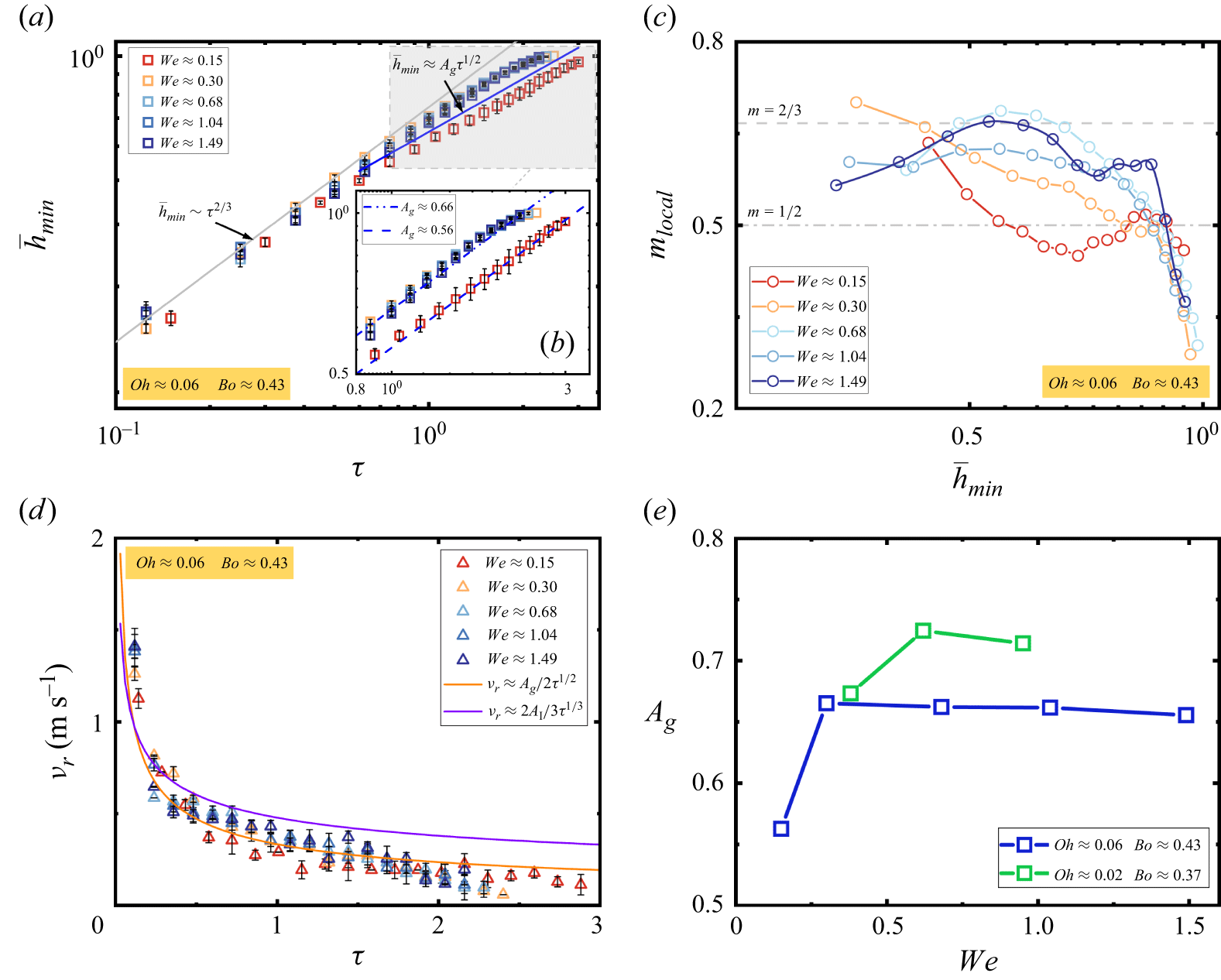
Neck contraction dynamics for different Weber numbers. (a) Dimensionless minimum radius
 $\bar {h}_{\textit{min}}$
versus dimensionless remaining time
 $\tau$
, compared with the theoretical power laws
 $\bar {h}_{\textit{min}}\sim \tau ^{1/2}$
and
 $\bar {h}_{\textit{min}}\sim \tau ^{2/3}$
. (b) Contraction factor
 $A_g$
in the
 $1/2$
-power-law regime as a function of
 $ \textit{We}$
, with corresponding fits. (c) Local power-law exponent
 $m_{\textit{local}} = \mathrm{d}\ln \bar {h}_{\textit{min}}/\mathrm{d}\ln \tau$
versus
 $\bar {h}_{\textit{min}}$
. (d) Radial contraction rate
 $v_r = \dot {{h}}$
versus
 $\tau$
, compared with the power laws
 $v_r \approx A_g / (2 \tau ^{1/2})$
and
 $v_r \approx 2 A_I / (3 \tau ^{1/3})$
. (e) Contraction factor
 $A_g$
versus
 $ \textit{We}$
for different Ohnesorge and Bond numbers.

Neck contraction dynamics for different Bond numbers. (a) Dimensionless minimum radius
 $\bar {h}_{\textit{min}}$
as a function of dimensionless remaining time
 $\tau$
, compared with the theoretical power laws
 $\bar {h}_{\textit{min}} \sim \tau ^{1/2}$
and
 $\bar {h}_{\textit{min}} \sim \tau ^{2/3}$
. (b) Contraction factor
 $A_g$
in the
 $\tau ^{1/2}$
scaling regime as a function of
 $ \textit{Bo}$
, with corresponding power-law fits. (c) Contraction factor
 $A_g$
versus
 $ \textit{Bo}$
for different combinations of the Ohnesorge and Weber numbers.

Figure 3. Long description
The image contains three panels, each depicting different aspects of drop formation dynamics in Newtonian fluids. Panel A: A scatter plot shows the dimensionless minimum radius as a function of dimensionless remaining time. The x-axis is labeled with the symbol tau, and the y-axis is labeled with the symbol h_min. The plot includes multiple data series represented by different symbols and colors, corresponding to different Bond numbers (Bo) ranging from 0.26 to 0.55. The plot also includes theoretical power-law fits with annotations indicating the power laws. An inset within this panel shows a zoomed-in view of the data in the scaling regime. Panel B: An inset shows local power-law fits of the dimensionless minimum radius h_min versus dimensionless remaining time τ in the 1/2-power-law regime, with the corresponding fitted contraction factors A_g. The graph includes multiple data series represented by different symbols and colors, corresponding to different Bond numbers. The plot also includes power-law fits with annotations indicating the power laws. Panel C: A line graph shows the contraction factor (A_g) versus Bond number (Bo) for different combinations of the Ohnesorge (Oh) and Weber (We) numbers. The x-axis is labeled Bo, and the y-axis is labeled A_g. The graph includes two data series represented by different symbols and colors, corresponding to different combinations of Oh and We numbers.
The Weber number (
 $ \textit{We}$
), which characterises the inertia-to-capillary force ratio, is critical for achieving dynamic surface-tension balancing. For
 $ \textit{We} \lt 0.1$
and
 $ \textit{Bo} \approx 1$
, the droplet is in a quasi-static dripping regime dominated by gravity and surface tension. We therefore restrict our attention to
 $ \textit{We} \gt 0.1$
, where inertia, surface tension and gravity are in dynamic balance. Figure 2 investigates the effect of
 $ \textit{We}$
(0.15, 0.30, 0.68, 1.04, 1.49) on neck contraction under
 $ \textit{Oh} \ll 1$
and
 $ \textit{Bo} \approx 0.43$
. Figure 2(a) shows the evolution of the minimum dimensionless neck radius
 $\bar {h}_{\textit{min}}$
with dimensionless remaining time
 $\tau$
. All curves exhibit a clear double-power-law behaviour: an initial
 $\bar {h}_{\textit{min}} \sim \tau ^{1/2}$
scaling followed by a transition to
 $\bar {h}_{\textit{min}} \sim \tau ^{2/3}$
scaling near breakup. In the early stage, the curves show strong
 $ \textit{We}$
dependence. The
 $ \textit{We} = 0.15$
curve lies noticeably below the others, indicating faster initial contraction due to surface-tension dominance. For
 $ \textit{We} \ge 0.30$
, the curves nearly coincide, suggesting that increasing inertia slows contraction and shifts the curves upward. As contraction proceeds, all curves converge to the
 $\tau ^{2/3}$
scaling, marking the entry into the inertial–capillary balanced regime. Figure 2(b) presents fits of the early-stage data to the
 $\tau ^{1/2}$
power law. The fitted contraction factor
 $A_g$
is smallest at
 $ \textit{We} = 0.15$
(
 $A_g = 0.56$
), increases rapidly to approximately
 $0.66$
at
 $ \textit{We} = 0.30$
and remains nearly constant for higher
 $ \textit{We}$
. This behaviour reflects the condition for dynamic surface-tension balancing, which requires
 $ \textit{We} \sim 1$
. At small
 $ \textit{We}$
, balancing is initially absent, leading to rapid surface-tension-driven contraction. As contraction proceeds, the local
 $ \textit{We}$
increases and balancing becomes established. Near
 $ \textit{We} \sim 1$
, inertia dominates, slowing contraction. The slight decrease in
 $A_g$
at the highest
 $ \textit{We}$
values suggests that excessive stretching may mildly disrupt the force balance. Figure 2(c) shows the local power-law exponent
 $m_{\textit{local}} = \mathrm{d}\ln \bar {h}_{\textit{min}} / \mathrm{d}\ln \tau$
as a function of
 $\bar {h}_{\textit{min}}$
. For
 $ \textit{We} = 0.15$
,
 $m_{\textit{local}}$
fluctuates around
 $0.5$
before gradually approaching
 $2/3$
. For
 $ \textit{We} \ge 0.30$
,
 $m_{\textit{local}}$
increases monotonically with decreasing
 $\bar {h}_{\textit{min}}$
, and larger
 $ \textit{We}$
accelerates the transition to the
 $2/3$
scaling. The early-stage plateau near
 $0.5$
is most prolonged for the smallest
 $ \textit{We}$
, consistent with the extended
 $\tau ^{1/2}$
behaviour observed in figure 2(a). Figure 2(d) plots the radial contraction rate
 $v_r = \dot {h}$
against
 $\tau$
for different
 $ \textit{We}$
. In the inertial–capillary equilibrium regime,
 $\bar {h}_{\textit{min}} \approx A_g \tau ^{1/2}$
, yielding
 $v_r \approx A_g / (2 \tau ^{1/2})$
; in the inertial self-similar regime,
 $\bar {h}_{\textit{min}} \approx A_I \tau ^{2/3}$
, yielding
 $v_r \approx 2 A_I / (3 \tau ^{1/3})$
. These correspond to the orange and purple curves, respectively. The data show a clear transition between the two power laws. Smaller
 $ \textit{We}$
delays the transition and maintains the
 $\tau ^{-1/2}$
scaling over a longer interval, while larger
 $ \textit{We}$
accelerates the transition, in agreement with the evolution of
 $m_{\textit{local}}$
shown in figure 2(c). Figure 2(e) compares
 $A_g$
as a function of
 $ \textit{We}$
for different
 $ \textit{Bo}$
and
 $ \textit{Oh}$
. Two datasets are shown: blue (
 $ \textit{Oh} \approx 0.06$
,
 $ \textit{Bo} \approx 0.43$
) and green (
 $ \textit{Oh} \approx 0.02$
,
 $ \textit{Bo} \approx 0.37$
). Both exhibit a rapid initial increase in
 $A_g$
followed by saturation, stabilising at approximately
 $0.66$
and
 $0.72$
, respectively. The blue curve lies below the green curve, indicating that the combined change in fluid properties, especially the increase in
 $ \textit{Oh}$
, reduces
 $A_{{g}}$
and leads to faster apparent contraction. Despite these quantitative differences, the overall trend – smallest
 $A_g$
at small
 $ \textit{We}$
– remains consistent with figure 2(b). In summary, the experimental data capture the complete transition from the surface-tension-balancing regime to the inertial–capillary regime during neck contraction. A key observation is that smaller
 $ \textit{We}$
prolongs the
 $\tau ^{1/2}$
scaling regime, as evidenced by the evolution of
 $\bar {h}_{\textit{min}}$
,
 $m_{\textit{local}}$
,
 $v_r$
and
 $A_g$
. This behaviour originates from the growth of
 $ \textit{We}$
during contraction: early-stage balancing requires
 $ \textit{We} \sim 1$
, and a smaller initial
 $ \textit{We}$
delays the onset of this condition, thereby extending the balancing-dominated window. Once
 $ \textit{We} \sim 1$
is reached, the system transitions more rapidly to inertial–capillary dominance. While viscous and gravitational effects (via
 $ \textit{Oh}$
and
 $ \textit{Bo}$
) influence the absolute value of
 $A_g$
, the control of
 $ \textit{We}$
over the duration of the
 $\tau ^{1/2}$
regime holds across different fluid properties.
The Bond number (
 $ \textit{Bo}$
) characterises the ratio of gravity to surface tension and captures the influence of finite gravity. Figure 2(e) shows that varying
 $ \textit{Bo}$
has a measurable effect on the contraction factor. Figure 3 further elucidates the role of
 $ \textit{Bo}$
in neck-contraction dynamics under moderate finite gravity (
 $ \textit{Bo} \lesssim 0.5$
), with measurements extending to
 $ \textit{Bo} \approx 0.55$
. Figure 3(a) shows
 $\bar {h}_{\textit{min}}$
versus
 $\tau$
for different
 $ \textit{Bo}$
values at fixed
 $ \textit{We} \approx 1$
and
 $ \textit{Oh} \approx 0.06$
. In the main dataset,
 $ \textit{Bo}$
was varied by changing the nozzle dimensions up to the
 $2.3\,\mathrm{mm}$
inner-diameter needle, with inner diameters of
 $1.6$
and
 $2.3\,\mathrm{mm}$
and corresponding outer diameters of
 $1.8$
and
 $2.8\,\mathrm{mm}$
. Across this moderate-
 $ \textit{Bo}$
dataset, the contraction curves still exhibit the same apparent transition observed in figure 2(a): an early
 $\tau ^{1/2}$
regime followed by a later inertial–capillary
 $\tau ^{2/3}$
regime. As
 $ \textit{Bo}$
increases, the contraction curves shift, indicating that finite gravity modifies the global drop shape and the initial stretching state. However, in this moderate-
 $ \textit{Bo}$
range, the influence of
 $ \textit{Bo}$
is mainly reflected in the contraction factor rather than in a measurable change of the apparent early-stage scaling exponent. Figure 3(b) presents local fits to the
 $\tau ^{1/2}$
region in figure 3(a), yielding
 $A_g$
as a function of
 $ \textit{Bo}$
. The fitted values are as follows: for
 $ \textit{Bo} = 0.26$
–
 $0.33$
,
 $A_g \approx 0.65$
(
 $R^2 = 0.99$
); for
 $ \textit{Bo} = 0.38$
–
 $0.55$
,
 $A_g \approx 0.70$
(
 $R^2 = 0.98$
). These results indicate high fit reliability and show that
 $A_g$
varies moderately with
 $ \textit{Bo}$
within the present parameter range. This suggests that moderate gravity can modify the contraction prefactor by changing the initial drop configuration, while still remaining subdominant in the local neck balance. Figure 3(c) further compares
 $A_g$
versus
 $ \textit{Bo}$
for two parameter combinations: the purple curve
 $(Oh \approx 0.01, We \approx 0.8)$
and the yellow curve
 $(Oh \approx 0.06, We \approx 1)$
. In both cases,
 $A_g$
varies only weakly and non-monotonically with
 $ \textit{Bo}$
: the purple curve changes from approximately
 $0.69$
to
 $0.74$
and then decreases to
 $0.68$
, while the yellow curve increases from approximately
 $0.65$
to
 $0.70$
before returning to
 $0.65$
. The purple curve generally lies above the yellow curve, indicating that lower
 $ \textit{Oh}$
and lower
 $ \textit{We}$
give a larger contraction factor and hence slower apparent contraction. Compared with this moderate variation in
 $ \textit{Bo}$
, the combined effects of viscosity and inertia have a stronger influence on
 $A_g$
. Collectively, the measurements within
 $ \textit{Bo} \lesssim 0.5$
show that the Bond number mainly provides a weak prefactor-level correction to
 $A_g$
, without measurably changing the transition from the early surface-tension-balancing regime
 $(\bar {h}_{\textit{min}}\sim \tau ^{1/2})$
to the inertial–capillary regime
 $(\bar {h}_{\textit{min}}\sim \tau ^{2/3})$
. Higher-
 $ \textit{Bo}$
cases were also analysed to assess the upper limit of this regime. Their local-exponent behaviour departs from the
 $1/2$
prediction of the present model, and the detailed analysis is given in the Supplementary Material, which is available at https://doi.org/10.1017/jfm.2026.11931.
Comparison of neck-contraction dynamics for different Ohnesorge numbers as a function of Weber number. (a) Dimensionless minimum radius
 $\bar {h}_{\textit{min}}$
versus dimensionless remaining time
 $\tau$
for different
 $ \textit{We}$
at
 $ \textit{Oh} \approx 0.14$
,
 $ \textit{Bo} \approx 0.37$
. (b) Local fits in the
 $1/2$
-power-law region of (a) and the corresponding contraction factor
 $A_g$
. (c)
 $\bar {h}_{\textit{min}}$
versus
 $\tau$
for different
 $ \textit{We}$
at
 $ \textit{Oh} \approx 0.55$
,
 $ \textit{Bo} \approx 0.40$
. (d) Local fits in the
 $1/2$
-power-law region of (c) and the corresponding
 $A_g$
. As
 $ \textit{Oh}$
increases, the surface-tension-balancing regime is significantly shortened,
 $A_g$
decreases and the system enters the viscosity-dominated linear contraction regime earlier.

Figure 4. Long description
The image contains four panels of graphs analyzing the neck-contraction dynamics for different Ohnesorge numbers as a function of Weber number. Panel A: A plot with data points, error bars, and fitted lines showing the dimensionless minimum radius (h_min) versus dimensionless remaining time (τ) for different Weber numbers (We) at Ohnesorge number (Oh) approximately 0.14 and Bond number (Bo) approximately 0.37. The plot includes data points for We values of 0.38, 0.63, and 0.96. Panel B: A line graph showing local fits in the power-law region of Panel A and the corresponding contraction factor (A_g). The graph includes lines for A_g values of 0.56, 0.58, and 0.59. Panel C: A plot with data points, error bars, and fitted lines showing the dimensionless minimum radius (h_min) versus dimensionless remaining time (τ) for different Weber numbers at Oh approximately 0.55 and Bo approximately 0.40. The plot includes data points for We values of 0.41, 0.68, and 1.04. Panel D: A line graph showing local fits in the power-law region of Panel C and the corresponding contraction factor (A_g). The graph includes lines for A_g values of 0.43 and 0.45. The graphs illustrate how the surface-tension-balancing regime shortens as the Ohnesorge number increases, leading to earlier entry into the viscosity-dominated linear contraction regime.
Sensitivity of the contraction factor
 $A_g$
to dimensionless numbers and the resulting dimensionless correlation. (a)
 $A_g$
versus
 $ \textit{We}$
for different
 $ \textit{Oh}$
. (b) Relationship between
 $A_g$
and the dimensionless combination
 $\varPi = We^{0.06} Bo^{-0.01} Oh^{-0.08}$
. The red line represents the empirical fit
 $\ln A_g = \ln k + \ln \varPi$
, and the black open circles denote the experimental data points.

The Ohnesorge number (
 $ \textit{Oh}$
) characterises the ratio of viscous forces to the combined inertial–capillary forces and plays a key role in disrupting the dynamic surface-tension balance. While figures 2 and 3 show that modest variations in
 $ \textit{Oh}$
non-negligibly affect the contraction factor
 $A_g$
in the
 $\tau ^{1/2}$
regime, a systematic examination of viscosity effects is presented in figures 4 and 5. An overview of the overall viscous effect on contraction timescales is provided in the Supplementary Material. Figure 4 explores the influence of
 $ \textit{Oh}$
on neck contraction dynamics at two representative viscosity levels. Figures 4(a) and 4(c) plot
 $\bar {h}_{\textit{min}}$
versus
 $\tau$
for
 $ \textit{Oh} \approx 0.14$
(with
 $ \textit{We} = 0.38$
,
 $0.63$
,
 $0.96$
) and
 $ \textit{Oh} \approx 0.55$
(with
 $ \textit{We} = 0.41$
,
 $0.68$
,
 $1.04$
), both at
 $ \textit{Bo} \approx 0.37$
–
 $0.40$
. For each fixed
 $ \textit{Oh}$
, the curves for different
 $ \textit{We}$
closely collapse, indicating that once the system enters the
 $\tau ^{1/2}$
regime, the influence of
 $ \textit{We}$
on the contraction path saturates. At
 $ \textit{Oh} \approx 0.14$
, a clear transition from the surface-tension-balancing regime to an inertial–viscous–capillary balanced regime is observed. At
 $ \textit{Oh} \approx 0.55$
, however, the balancing regime is drastically shortened – becoming nearly invisible – and the later regime, characterised by a power law approaching
 $\bar {h}_{\textit{min}} \sim \tau$
, dominates the contraction. Figures 4(b) and 4(d) present fits to the
 $\tau ^{1/2}$
scaling for the two datasets. At
 $ \textit{Oh} \approx 0.14$
,
 $A_g$
values range from
 $0.56$
to
 $0.59$
(
 $R^2 \gt 0.99$
), showing a slight decrease with increasing
 $ \textit{We}$
. At
 $ \textit{Oh} \approx 0.55$
,
 $A_g$
values are significantly lower, ranging from
 $0.43$
to
 $0.46$
(
 $R^2 \gt 0.99$
), and exhibit a weak increase with
 $ \textit{We}$
before stabilising. Although the fit quality remains high at
 $ \textit{Oh} \approx 0.55$
, the fitting window is greatly shortened, and the balancing regime accounts for only a minimal fraction of the total contraction time. This suggests that at high viscosity, initial balancing is at best nominal and brief. Collectively, figure 4 demonstrates that at
 $ \textit{Oh} \approx 0.14$
, a distinct balancing regime exists with
 $A_g \approx 0.56$
–
 $0.59$
, followed by a transition to an inertial–viscous–capillary balanced regime. At
 $ \textit{Oh} \approx 0.55$
, enhanced viscosity nearly eliminates the balancing regime (
 $A_g \approx 0.43$
–
 $0.46$
), and the system enters a viscosity-dominated linear contraction regime much earlier.
Figure 5 quantitatively analyses the sensitivity of the contraction factor
 $A_g$
to the governing dimensionless numbers. Figure 5(a) shows
 $A_g$
as a function of
 $ \textit{We}$
for two fixed
 $ \textit{Oh}$
values:
 $0.14$
and
 $0.55$
. At
 $ \textit{Oh} = 0.14$
,
 $A_g$
increases slowly and then stabilises as
 $ \textit{We}$
increases. At
 $ \textit{Oh} = 0.55$
,
 $A_g$
also increases slowly and then stabilises, but the entire curve lies below that for
 $ \textit{Oh} = 0.14$
, indicating that increased viscosity significantly reduces
 $A_g$
. In summary, the dependence of the contraction factor
 $A_g$
on the dimensionless numbers can be summarised as follows. With increasing
 $ \textit{We}$
,
 $A_g$
varies weakly and generally increases slightly, indicating a weak positive correlation with inertia. Increasing
 $ \textit{Oh}$
reduces
 $A_g$
, showing that viscosity narrows the balancing region and accelerates the apparent contraction. Within the moderate finite-gravity range considered here, the variation of
 $A_g$
with
 $ \textit{Bo}$
is comparatively weak, suggesting that gravity mainly provides a prefactor-level correction rather than acting as a dominant control parameter. Based on these observations, a dimensionless combination
 $\varPi = We^{a} Bo^{b} Oh^{c}$
is proposed to describe
 $A_g$
in a unified manner. Multivariate nonlinear regression using experimental data across different
 $ \textit{Oh}$
,
 $ \textit{Bo}$
and
 $ \textit{We}$
yields
 $a = 0.06$
,
 $b = -0.01$
and
 $c = -0.08$
, i.e.
 $\varPi = We^{0.06} Bo^{-0.01} Oh^{-0.08}$
. Figure 5(b) plots
 $\ln A_g$
versus
 $\ln \varPi$
, together with a linear fit
 $\ln A_g = \ln k + \ln \varPi$
. The fit gives
 $k = 0.49$
with a coefficient of determination
 $R^2 = 0.77$
. Despite some scatter, the overall agreement supports the use of this empirical correlation within the present parameter range. This correlation provides a quantitative prediction for
 $A_g$
in the surface-tension-balancing regime and shows that
 $A_g$
is weakly enhanced by inertia, reduced by viscosity and only weakly affected by
 $ \textit{Bo}$
within the moderate finite-gravity range.
4. Conclusion
By combining theoretical modelling and high-speed photography, this work investigates pendant-drop neck contraction under moderate finite gravity (
 $ \textit{Bo}\lesssim 0.5$
). The main conclusions are as follows. A theoretical model for the dynamic surface-tension-balancing regime yields the scaling law
 $h\sim \tau ^{1/2}$
, independent of viscosity, with the initial condition
 $ \textit{We} \sim 1$
, and the associated scalings
 $\dot {h} \sim \tau ^{-1/2}$
and
 $L \sim \tau ^{-1}$
. Experiments verify a three-stage evolution from dynamic balancing to inertial–capillary equilibrium and self-similarity. Within the present Bond-number range,
 $ \textit{Bo}$
mainly provides a weak prefactor-level correction to
 $A_{\mathrm{g}}$
, while the contraction dynamics remain consistent with the apparent transition from the
 $\tau ^{1/2}$
regime to the
 $\tau ^{2/3}$
regime. The coupled regulatory laws are clarified: smaller
 $ \textit{We}$
prolongs the balancing regime and reduces
 $A_g$
, while larger
 $ \textit{Oh}$
narrows the balancing window and reduces
 $A_g$
. The empirical correlation
 $A_g = 0.49\,We^{0.06}Bo^{-0.01}Oh^{-0.08}$
with
 $R^2 = 0.77$
shows that
 $A_g$
is weakly enhanced by inertia, reduced by viscosity and only weakly affected by
 $ \textit{Bo}$
in this range. This work identifies the range of validity of a dynamic surface-tension-balancing law in the non-self-similar contraction regime under finite but non-dominant gravity and provides a quantitative description of the contraction factor under coupled inertial, viscous and gravitational effects.
Supplementary materials and movies
Supplementary materials and movies are available at https://doi.org/10.1017/jfm.2026.11931.
Funding
This study is supported by the National Natural Science Foundation of China (Grant No. 12172094).
Declaration of interests
The authors report no conflict of interest.

 R
 R1
 R
 h¯min
 L
 t0=tb−t
 tb
 Oh≈0.06
 We≈1.04
 Bo≈0.43
 t0=tb−t
 t0=20.6ms
 t0=0

 25±1∘C
 h¯min
 τ
 h¯min∼τ1/2
 h¯min∼τ2/3
 Ag
 1/2
 We
 mlocal=dlnh¯min/dlnτ
 h¯min
 vr=h˙
 τ
 vr≈Ag/(2τ1/2)
 vr≈2AI/(3τ1/3)
 Ag
 We

 h¯min
 τ
 h¯min∼τ1/2
 h¯min∼τ2/3
 Ag
 τ1/2
 Bo
 Ag
 Bo

 h¯min
 τ
 We
 Oh≈0.14
 Bo≈0.37
 1/2
 Ag
 h¯min
 τ
 We
 Oh≈0.55
 Bo≈0.40
 1/2
 Ag
 Oh
 Ag

 Ag
 Ag
 We
 Oh
 Ag
 Π=We0.06Bo−0.01Oh−0.08
 lnAg=lnk+lnΠ



