


Introduction
Rising unemployment and poverty due to globalization,Footnote 1 structural changes in the economy,Footnote 2 automation, Footnote 3 and other reasons revealed the shortcomings of the welfare state and its social security systems. Footnote 4 In search of justice in income distribution and easy access to necessities by everyone, basic income (BI) has become one of the main topics of conversation. BI has long been addressed from different points of view. There are diverse interpretations and suggestions for an unconditional income granted to citizens. Nevertheless, besides the moral principle, the subject has been popularized in the economic literature since the 1960s. Many authors discuss its impacts on freedom, economy, labor market, and income distribution Footnote 5 together with its social feasibility and its effects on psychological well-being from different political and economic backgrounds. Footnote 6 The impacts of the recent Covid-19 pandemic on the labor markets also draw attention to social policies. Footnote 7 Besides economics, the need for a BI finds a voice in other disciplines. In their recent study, Johnson etal. draw attention to the social and economic impacts of the Covid-19 pandemic, such as unemployment and homelessness. Footnote 8 Authors suggest that BI solves the possible intergenerational trauma that can arise due to the pandemic.
Since there is no single inventor of BI, there are several names: guaranteed income, unconditional basic income, universal basic income, social dividend, or demogrant. Philippe van Parijs defines BI as “an income paid by a political community to all its members on an individual basis, without means test or work requirement.” Footnote 9 Contrary to the welfare state, which aims for every member of the population to work, BI does not require work incentives or even a work record.
There are many reasons behind the suggestion of BI: rising income inequality, the declining income share of labor, the process of robotization in manufacturing, service, and other industries, and growth without employment.Footnote 10 Similar trends in the economy forced people to seek liberty and equality and fight against unacceptable working conditions.
BI policy has many advantages. Giving a chance of getting basic needs to all people, elimination of poverty, decreasing the need for and the costs of bureaucracy, making the employer–employee relationship more symmetrical via increasing employee’s bargaining power, and rewarding volunteer work or the housework done mainly by women—which are not paid in the market—are some of them.Footnote 11 BI policy lowers the uncertainty of households by lowering bureaucratic costs generated by means-tested policies (the bureaucratic costs of transfers in Turkey are reported to be $857 million by the Turkish Statistical Institute (TurkStat) for 2017). It can also be related to unpaid labor in housework that is mostly done by women. With a BI policy, the bargaining power of labor increases since their reservation wage increases. As is discussed further, implementations have shown that it also shifts the labor supply curve upwards and does not increase leisure demand. Finally, eliminating poverty would save money spent on healthcare and reduce crime-prevention costs.Footnote 12
A current BI experiment may provide more reliable information on the positive implications of such policy. The experiment was in progress in Canada. The Ontario Basic Income Project started in 2017 with 4,500 recipients between the ages of 18 and 64. Footnote 13 Recipients are not randomly selected, yet they have to be living on a low income. The income tax on market income is 50 percent. After the project ended in March 2019, Basic Income Canadian Network (BICN) conducted a survey and asked twenty-two questions to 400 participants, constituting 9.4 percent of total recipients. Footnote 14 According to the results, 88 percent of respondents reported less stress and anxiety. At the beginning of the pilot project, 81 percent of participants reported stress; 58 percent of the respondents reported improved house quality; 34 percent reported better transportation to work, childcare opportunities, or chance to start their businesses; 32 percent of them upgraded their educational background; 46 percent of them paid their debts; 74 percent of respondents accessed healthy food; and 45 percent reported fewer problems related to their health. However, 80 percent of them started to face their previous problems after the pilot’s cancellation, and 61 percent had to cancel their plans. As another recent example, Finland granted €560 per month to 2,000 unemployed citizens between the ages of 25 and 58. Footnote 15 BI payment is exempt from taxation and continues in case the recipient becomes employed. The experiment was in progress during 2017 and 2018. After a year, preliminary results show that recipients had better well-being with less stress and health problems and increased concentration. However, there have been no effects on employment.
There are also objections to the BI proposal. Reduction in work incentives is one of the reasons for these objections. The reduction happens due to high tax rates for financing the schemeFootnote 16 or the free-riding behavior with increasing nonwage income.Footnote 17 It is also criticized for being too expensive to be feasible or too little to be effective, and thus for being cost-ineffective.Footnote 18
Although some studies analyze a means-tested minimum incomeFootnote 19 with different amounts and coverage for Turkey,Footnote 20 there is no other analysis of the cost and income effect of BI to our knowledge. Considering all the critical aspects above, we estimate the cost of a possible BI scheme in Turkey. We aim to shed light on the topic in a way that will also benefit other developing countries. The data set we use is individual-level microdata which are obtained from surveys by TurkStat. It enables us to perform a static tax–benefit microsimulation that analyzes the households’ before- and after-policy incomes. The study continues with the evaluation of different approaches in the literature and analyzes implementations from around the world. After a short review of Turkey’s social policy and income distribution, it calculates the cost of possible BI scenarios for the country and evaluates its distributional effects. Findings show that a BI equal to the poverty line for the individuals aged 15 or above and equal to 30 percent of the poverty line for children below 15 leads to a reduction in the poverty rate from 12.43 percent to zero, the Gini index from 0.388 to 0.181, and the Theil index from 0.302 to 0.065. While the cost of this plan is equal to 17.77 percent of the gross domestic product (GDP), it can be covered solely by multiplying the current income tax by 3.54. Note that this tax is for the market income, and it does not apply to BI. When we consider BI, the effective tax rate increases less than this factor, especially for the relatively poor. The results section presents the detailed results and the other three scenarios and discusses them.
Review of the literature and implementations from the world
BI has been discussed worldwide, and there have been several experiments. This section presents some critical implementations from the around world and evaluates their results after reviewing the literature.
To our knowledge, although there are several descriptive studies on the topic, there is no study that estimates the costs or benefits of a BI policy in Turkey. Ayşe Buğra and Tolga N. Sınmazdemir’s study calculates the cost of granting an income to poor households in Turkey. Footnote 21 The cost-to-GDP ratio is investigated in twenty-four scenarios covering four different minimum income amounts and six different poverty lines. The most affordable scenario covering the monthly food expenditure of a poor household costs 0.06 percent of GDP, whereas the most expensive scenario in which the monthly payment is equal to half of the minimum wage costs 2 percent of GDP. However, this study analyzes means-tested minimum income rather than BI as in our study. Therefore, the costs of analyses are not comparable. Another minimum wage study for Turkey employs the Statistics on Income and Living Conditions data for 2007 and examines a scenario in which all eligible households are provided with 40 percent of the median income.Footnote 22 While eligibility varies among alternative definitions of the poor, the costs of introducing a minimum income scheme vary between 0.33 percent and 2.69 percent of GDP. In the most comprehensive scenario, households below 60 percent of the median income are granted an income subsidy that tops up their income to the threshold, and it costs 2.69 percent of GDP. As a result of this policy, the Gini coefficient decreases from 0.411 to 0.360. Although being informative and comprehensive, this study’s aim is far from that of ours. Therefore, we look for similar estimations for other economies.
Based on 2002 data, Charles M. A. Clark estimates the cost of BI for the USA. The amount of BI is fixed at the poverty threshold for individuals to bring all older adults above the threshold. Footnote 23 Children receive 37 percent of the amount that adults are granted. An essential point of this scheme is that the existing tax and benefit systems remain. A flat tax of 35 percent funds the extra cost of BI without creating a budget deficit. This scheme has a positive effect on income distribution. The Gini coefficient decreases from 0.418 to 0.339 thanks to the implementation of BI. The bottom four quintiles have an increase in income with BI. The only exception is the top quintile, which has a loss in income share by the bottom four’s gain. With progressive taxation instead of a flat rate, results could be even better. Micheal Collins estimates the cost of BI for Ireland by using survey data. Footnote 24 In this study too, the amounts that children and adults receive are differentiated, and the system is financed with a flat tax rate of 44 percent. Jordi Arcarons, Panella Daniel Raventos, and Melich Lluis Torrens introduce a similar analysis for Catalonia by using 2010 microdata, and find that an annual payment above the poverty threshold to adults and one-fifth of it to children is an attainable scheme with a 50 percent flat-rate income tax. Footnote 25 The Gini index decreases from 0.366 to 0.246 with the BI payments and the flat tax. In another study, Karl Widerquist estimates the cost of BI for the USA and finds that a marginal tax rate of 50 percent could finance a plan of $12,000 for adults and $6,000 for children. Footnote 26 The scheme reduces the poverty rate from 13.5 percent to nearly zero, similar to our results. These estimations require a flat tax rate of 37–50 percent and do not shift the burden to the middle-income households much more than the before-policy situation. In our estimations, however, progressive taxation is required for the middle-income households not to be net payers of this scheme. Therefore, to preserve progressivity, we left the tax brackets untouched but raised the rates proportionally.
Besides the estimations in the studies above, the implementation of BI policies around the world may provide guidance for a conceivable BI policy in Turkey. Such implementations are also essential references that provide information on labor supply decisions. The Alaska Permanent Fund, which was founded in 1976, is the most stable experiment in history. Footnote 27 Prudhoe Bay in Alaska is the largest oilfield in North America. At least one-fourth of the oil revenues are directed to the fund, and 90 percent of the state population (currently 670,000 citizens) meet the residency requirement regardless of their age, working situation, or another status to benefit from the fund since 1982. The amount of the payment reflects oil prices. It has been between $1,000 and $2,000 for the last twenty years. Damon Jones and Ioana E. Marinescu investigate the fund’s impact on the labor market. Footnote 28 Their findings show that implementing this policy has not reduced employment; it increased part-time employment instead. David Calnitsky and Jonathan P. Latner analyze the Manitoba Basic Annual Income Experiment launched in Dauphin, Manitoba, Canada, between 1975 and 1977. Footnote 29 During the experiment, each family is given 38 percent of the family’s median income. The amount of payment reflects household type and size. The negative income tax on market income was set at 50 percent. According to the study, the reduction in labor market participation is 11.3 percent. It is largely by single and older people, due to educational or health issues. On the other hand, Evelyn L. Forget shows that Dauphin students were more likely to stay in high school than other students in Manitoba during the experiment period. Footnote 30 Iran started to pay 28 percent of the median per capita household income in 2011 to about 75 million people. The removal of energy subsidies partly finances this amount, around 6.5 percent of GDP. Using the Household Expenditures and Income Survey microdata set, Djavad Salehi-Isfahani and Mohammad H. Mostafavi-Dehzooei employ difference-in-differences and fixed effects methods. Footnote 31 They find that women and self-employed men increased their weekly labor supply by more than half an hour.
Considering that the future of the capitalistic market economy is prone to financial and economic crises, scholars like Thomas Piketty Footnote 32 and Joseph E. Stiglitz Footnote 33 highlight wealth and income inequalities and advise a global wealth tax. At this point, a BI grant would be a reasonable and relevant policy to achieve equality and stability. It is already implemented in various types of economies with varying coverage. Turkey, as a developing country with challenging features for BI, such as a large population, high levels of youth unemployment, and high levels of poverty, would be an informative example for other economies, especially for developing economies. The lack of a comprehensive study that estimates the cost and benefit effects of a possible BI policy for a developing country like Turkey shaped this study’s subject and focus. Therefore, in the next section we analyze the social policy in Turkey before discussing the results of particular scenarios of a BI policy simulation in the following sections.
Social policy in Turkey
Turkey has a population of 80,810,515, of which 68 percent were of working-age in 2017, the year of the most recent data set. There are 22,676,186 households in the country, and 3,491,148 of them are single-person households. A total of 13.26 million people are granted social benefits of $46,105 million. This amount includes administration costs and other expenditures of $857 million, which could also be eliminated by implementing a BI policy. We use the current exchange rate of USD/TRY=8.30 (April 2021).
Some people in our data set receive more than one benefit. In 2017, pension and old-age payments received the most significant amount of benefits ($22,293 million), followed by healthcare benefits ($12,419 million) and benefits to survivors ($5,383 million). Table 1 shows the amounts of payments and the number of recipients by type of social benefits.
Social benefits in Turkey (2017)

Source: Turkish Statistical Institute, Income and Living Conditions Survey Microdata Set, 2019.
Given the figures in Table 1, we now take a look at the historical process and institutional background of the country’s social policy. Ayşe Buğra states that Turkey’s social security system was put in place in the era of regulated capitalism and welfare state development. In contrast, the reform of this system and the more recently introduced social assistance policies to the poor are situated in the global political economy of unregulated capitalism.Footnote 34 Consisting cash transfers and other social assistance payments, the Turkish welfare system has the logic of charity rather than the logic of citizenship, and it suffers from inequalities of class and gender. Supporting the cost of private daycare as a factor discouraging women’s labor force participation is an example of these inequalities. The crucial point is, according to Buğra, that the system does not have the achievement of equality as an objective. Conversely, the BI policy may have crucial importance in avoiding these inequalities and achieving equality in society.
To examine this subject within a theoretical framework, we should refer to Gøst Esping-Andersen’s The Three Worlds of Welfare Capitalism.Footnote 35 In his seminal work, the author describes three welfare regimes in relation to their inclusion of the state, family, and market as interacting actors in social risk protection. According to this theory, liberal regimes intend to provide means-tested assistance to low-income households, usually those that are working class. It offers market solutions to social problems either by guaranteeing a minimum or by directly subsidizing welfare payments. On the other hand, conservative regimes have family values at the core; thus, they comprise family-based assistance that exclude non-working wives from social insurance and provide family benefits that encourage motherhood. Finally, social democrat regimes are universalistic systems that promote equality of high standards. They aim to socialize the costs of caring for children, the aged, and the helpless instead of leaving this responsibility to the family’s capacity to support.
Acknowledging that Esping-Andersen’s theory is based mainly on western European states, alternative typologies are constructed as extensions to the three typologies discussed above. While the East Asian welfare state is a mix of liberal and conservative models, we are more interested in the southern European welfare state type, including Italy, Spain, Portugal, and Greece. In this model, there is a conservative characteristic that aims for family-based social assistance, and there is also governmental support for the young unemployed. In their study, Martin Powell and Erdem Yörük provide a meta-analysis that groups the existing studies on Turkey’s welfare regime by the way they classify the country within the framework of Esping-Andersen’s extended typologies.Footnote 36 Their results show that Turkey is usually classified as part of the southern European welfare regime. Yakut-Cakar etal. also highlight the similar characteristics of the welfare regime in Turkey compared to its southern European counterparts.
If we take a closer look at Turkey’s social insurance institutions before the reform in 2008, as Ayşe Buğra states, workers with different statuses at work were provided with diverse health and old age benefits: Civil Servants’ Retirement Chest and Social Insurance Organization for private sector employees. In 1971, the pension system Bağ-Kur was introduced to cover the self-employed. Means-tested health insurance for the poor, the Green Card, was introduced in 1992. Then, in 2008, Social Security Organization was established as a unified institution for workers with various statuses. It can be regarded as a move against the underlying inequalities of the former three-pillar system since it restructures the welfare payments and coverage from being employment based to income based. A plausible BI policy would be in the same direction as the reform. It would also be a remedy to the underlying inequalities of the current system. It would eliminate the financial dependencies of family members and eliminate the dependency of social protection on employment status or working record, and turn it from being market based to being citizenship based.
Data and methodology
In this part of the study, the distributional consequences of a possible BI policy are assessed employing a tax–benefit microsimulation model. The BI is assumed to be financed entirely by increasing the income tax. The data used for this purpose come from the Income and Living Conditions Survey Microdata Set of TurkStat, which covers 78,015 individuals (58,744 of working age) who were members of 22,869 households in 2017. Footnote 37 This data set is the most recent one available. The data set was published in 2019; however, surveys were conducted in 2017. These individual-level microdata were obtained from surveys and cannot be accessed online without permission. They are used in income distribution analyses since they provide individual- and household-level information on the income by source and type, education, health, and employment. Since it is a random sample from the population, results can be generalized to the population in many cases. There are also informal workers in the data set, and it makes us automatically account for the informality of employment.
It is essential to clarify that the analysis of personal income distribution and poverty is done using microdata only. Therefore, the sample in this part of the analysis is the sample in the microdata set. The data set includes a coefficient for each individual and household, extending analysis from sample to population. It is merely a weight parameter that measures the power of the sample to represent the whole population. However, these coefficients are habitually misleading when working on variables other than household size, for example, household incomes, social benefits, pensions, and tax estimations. Therefore, calculations are confined to the coverage of the data set.
The microdata set of TurkStat provides information on disposable income and social benefits both at the individual level and household level. Working with extensive, countrywide, individual-level data allows us to make more reliable comparisons using after-tax incomes. It also enables us to abide by the definition of BI and evaluate a non-means-tested policy. Since this study estimates the impacts of a BI policy assuming that BI is financed by income tax, it is crucial to recalculate disposable income after a change in income tax rates. So, the gross incomes of individuals are estimated using the information on their net income, then the rate of the income tax required to finance the BI is calculated.
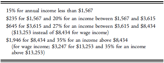
In 2017, income tax rates were imposed in as shown in Table 2. Using this information, gross income is estimated from net income.
Income tax rates (2017)

Source: Turkish Statistical Institute, Income and Living Conditions Survey Microdata Set, 2019.
Reversing the calculations in Table 2, the gross income of individuals is estimated as follows:
 $$GI = {1 \over {0.85}}{\rm{*}}NI\quad{\rm{if}}\,\,\left( {{1 \over {0.85}}{\rm{*}}NI} \right) < 1,567,$$
 $$GI = \left[ {{1 \over {0.80}}{\rm{*}}\left( {NI - \left( {1,567 - 235} \right)} \right)} \right] + 1,567\,\quad{\rm{if}}\,\,1,567 \le \left[ {\left[ {{1 \over {0.80}}{\rm{*}}\left( {I - \left( {1,567 - 235} \right)} \right)} \right] + 1,567} \right] < 3,615,$$
 $$GI = \left[ {{1 \over {0.73}}{\rm{*}}\left( {NI - \left( {3,615 - 645} \right)} \right)} \right] + 3,615\quad{\rm{if}}\,3,615 \le \left[ {\left[ {{1 \over {0.73}}{\rm{*}}\left( {NI - \left( {3,615 - 645} \right)} \right)} \right] + 3,615} \right] < 8,434,\;$$
 $$GI = \left[ {{1 \over {0.65}}{\rm{*}}\left( {NI - \left( {8,434 - 1,946} \right)} \right)} \right] + 8,434\quad{\rm{if}}\,8,434 \le \left[ {\left[ {{1 \over {0.65}}{\rm{*}}\left( {NI - \left( {8,434 - 1,946} \right)} \right)} \right] + 8,434} \right],$$
where
 $GI$
is the gross income,
 $NI$
is the net income, and the unit is US dollars. Note that this calculation is for the proprietors’ income. For the wage income, we use the amounts 3,247 and 13,253 instead of 1,946 and 8,434, respectively.
The main idea of our methodology is that the additional cost of BI is covered by the income tax payments of the individuals. To make it more straightforward, think of a simple example of an economy in which there are
 $I$
individuals and each individual
 $i$
has a gross income of
 $G{I_i}$
, a net income of
 $N{I_i}$
, an initial tax payment of
 ${T_i} = G{I_i} - N{I_i}$
, and an initial tax rate of
 ${t_i} = {T_i}/G{I_i}$
. Regardless of the number of tax brackets, each taxpayer has its tax rate since their gross and net incomes may well differ. When a BI is granted to each individual, its additional cost to the economy is collected from individuals by increasing their income tax equally (it is simply a redistribution among individuals). Therefore, the additional cost of the BI payments is equal to the difference between the new tax payments,
 ${T_i}'$
, and the initial tax payments:
 $$\mathop \sum \nolimits_i^I B{I_i} = \mathop \sum \nolimits_i^I {T_i}' - \mathop \sum \nolimits_i^I {T_i}$$
Since the BI payments are equal for each individual, the left-hand side of the equation can be rewritten as follows for simplicity:
 $$I*BI = \mathop \sum \nolimits_i^I {T_i}' - \mathop \sum \nolimits_i^I {T_i}$$
Note that we stated above that we increase the tax rate of individuals equally to cover the cost of BI. Suppose that the tax rate of each individual is multiplied by a factor
 $f = {T_i}'/{T_i}$
. Therefore, the equation above becomes
 $$I*BI = \mathop \sum \nolimits_i^I \left( {f*{T_i}} \right) - \mathop \sum \nolimits_i^I {T_i}$$
Rearranging the equation, we get
 $$I*BI = \left( {f - 1} \right)\mathop \sum \nolimits_i^I {T_i}$$
The left-hand side of the equation is the total cost of BI, and the right-hand side of the equation is the total initial tax collection multiplied by
 $f - 1$
. The factor
 $f$
is also equal to the ratio of the total cost of BI to the total initial tax collection. Given the recipients and the amount of BI and initial taxes, which are already known, we can calculate the required increase in the income tax rate, namely the factor
 $f$
.
Using the information on the BI payments,
 $B{I_i}$
, and new tax rates,
 $\left( {f*{t_i}} \right)$
, we can calculate the after-policy net income of each individual and Gini and Theil indices and other statistics on distributions such as P90/P10, P90/P50, and S80/S20. P90/P10 is the ratio of the ninth decile’s upper bound value to that of the first decile of income. Similarly, P10/P50 is the ratio of the first decile’s upper bound value to the median income. S80/S20, on the other hand, is the ratio of the average income of the wealthiest quintile to that of the poorest quintile of the population. With these five indicators, one can observe the change in income distribution with high sensitivity. While the Gini coefficient focuses more on the middle part of the distribution, the Theil index puts larger weights on tails. Therefore, the Theil index gives us more sensitive results in the analysis of the poor’s well-being. However, since the policy change would affect the whole population, the Gini coefficient is still a helpful indicator.
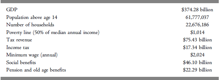
Using the microdata set, the median income and the poverty line are calculated. The poverty line is determined as half of the median income, approximately equal to $1,014. Households with annual equivalent income below this level are classified as poor. Social benefits paid to individuals and households are calculated as well.
As well as reporting the effect of the policy on income distribution, the study also analyzes the change in income of the slices of the population and the poverty rate. Households are separated into ten income groups, and after granting BI and imposing the new income tax the change in each group’s income is calculated. Therefore, gainers and losers from the policy change are detected, and income distribution among groups is reported. Note that the before-policy poverty line is used because if a new line is calculated, before- and after-policy situations would not be comparable. In the same way, income groups are held the same as before the policy to analyze the impact on their incomes.
Two different amounts, the poverty line ($1,014) and half of it, are chosen as the amount of the BI payment. In the next step, the receiver of the payment is determined. BI can be granted at the individual and household levels. For the individual-level analysis, every adult aged 15 or above is granted the full amount, while children younger than 15 are granted 30 percent of the full amount. When we make a household-level analysis, each household is granted the full amount multiplied by its equivalence scale. An equivalence scale is a valuable tool for comparing households of different sizes. It is calculated as the weighted sum of the number of individuals in the household. Weights are 1, 0.5, and 0.3 for the reference person, other adults, and children, respectively. The calculation of the equivalence scale can be shown as follows:
 $$e = \left( {1 + 0.5*\left( {{n_a} - 1} \right) + 0.3*\left( {{n_c}} \right)} \right)$$
where
 $e$
is the equivalence scale,
 ${n_a}$
is the number of adults in the household, and
 ${n_c}$
is the number of children in the household. Now we can calculate equivalent income for the household,
 ${y_d}$
, by dividing the disposable household income,
 ${Y_d}$
, by the equivalence coefficient,
 $e$
:
 $$$${y_d} = {{{Y_d}} \over e}$$$$
Therefore, when the BI is granted to the household instead of the individual, each household receives
 $BI*e$
amounts of dollars, and thus the equivalent income of the members of the household increases exactly by
 $BI$
.
The choice of the amount and recipients gives us four different cases. The distributional impacts and costs of each case are reported in Table 4. In all cases, income distribution is analyzed on the household level by using the equivalent income.
Selected macroeconomic indicators of Turkey (2017)

Source: Turkish Statistical Institute, Income and Living Conditions Survey Microdata Set, 2019.
Implications of the scenarios

Source: Turkish Statistical Institute, Income and Living Conditions Survey Microdata Set, 2019.
Results
From a macroeconomic view, it can be seen from Table 3 that Turkey has a large population size with substantial poverty. It makes it quite expensive to grant a BI payment. Since our first aim is to redistribute income to obtain an equal distribution, we did not impose an upper limit on the tax rates and let the model yield the required tax rates given the amount of the payment. However, we created alternative scenarios with lower levels of BI payment and households as recipients to examine more feasible cases. We then interpret their income-distributional implications.
In 2017, tax collection was roughly $75.43 billion (including $17.34 billion in income tax), and $46.1 billion was given to the public as social benefit, $22.29 billion as pension and old-age benefits. Our study utilizes the income tax as the potential source of financing BI and introduces a model to finance BI payments with additional income tax imposed on individuals.
Table 4 presents the results for four different cases. For comparison, the current value of indicators is reported as well. The Gini index for Turkey was 0.388 in 2017. The Theil index was 0.302, and 12.43 percent of households were living below the poverty line. In the third and fourth columns of Table 4 (titled “Individual”), the costs and implications are estimated for the annual BI payment granted to each individual. In these scenarios, the individuals aged 15 or above are granted the full amount, equal to the poverty line ($1,014) in the third column and half of it ($507) in the fourth column. In the fifth and sixth columns (titled “Equivalent”), the same calculations are then performed for another scenario in which the recipient of BI is the household. In these scenarios, the household is granted the full amount or half of it (as in the “Individual” scenarios) multiplied by the equivalence scale of the household. By multiplication, we control for household size and ensure that regardless of the size of the household, any member of any household has the same equivalent income. For instance, consider a family consisting of two adults and two children. This family’s equivalence scale is
 $1 + 0.5 + \left( {0.3*2} \right) = 2.1$
, where factor 1 is for the first adult in the household, 0.5 is for the second adult, and 0.3 for each of the children. In the third scenario (fifth column of Table 4), this family is granted a BI of
 $\$ 1,014*2.1 = \$ .2,129.4$
. Therefore, given that the household does not have any market income, the equivalent income of the household (the total income divided by the equivalence scale) is still $1,014, which means that the household is at the poverty line and counted as non-poor.
As Table 4 shows, the fourth case does not decrease poverty as much as we expect from such a payment. The second case even slightly increases the poverty rate. The reason behind this situation is that middle-income households pay taxes in large amounts to finance the relatively lower amount of BI payment. Therefore, they become net payers and fall below the poverty line while others climb up to the line. In the second case, the number of households falling below the poverty line is higher than the number of households ending above the poverty line. Thus, the poverty rate slightly increases; the only thing that changed is who is poor. These scenarios show that BI should be high enough, or a more progressive tax scheme should finance it. Remember that we do not have the super-rich in our data set, and we do not have taxes other than income tax as the source of finance. Hence, under these circumstances, these scenarios are unfeasible.
In the first and third scenarios in Table 4, the amount of BI payment is equal to the poverty line. Note that, in the third scenario, we grant BI to the household rather than the individual, and we multiply the initial amount of BI payment by the equivalence scale of the household. Therefore, each household escapes from poverty, and poverty is eliminated. In the first scenario, most households reach an income level even above the poverty line since the payment is made at the individual level.
We want to focus on the first (original) scenario as it grants BI payment at the individual level. This scenario decreases the Gini index from 0.388 to 0.181, which means a considerable amount of redistribution. The Theil index falls even more, from 0.302 to 0.065. It means that there is more distribution at the tails of the distribution. This is as expected because the BI payment tops up the income of the poorest part of the population by eliminating poverty while the high rate of income taxes trims the income of the richest. The effect of the policy can also be seen in the P90/P10, P10/P50, and S80/S20 ratios. More than half of the households are net receivers. Looking at the net payers and net receivers in more detail, we see that the top 40 percent of the population face decrease in their incomes, whereas those at the bottom see their incomes rise significantly.
Figure 1 shows the income distribution before and after the policy change. The solid line shows the distribution before the BI policy, while the dashed line shows the distribution after BI payments and tax reform. After-policy distribution is truncated at the poverty line level (the dotted vertical line) since non-taxable BI payments eliminate poverty. The new distribution has two peaks, the higher one has resulted from after-tax incomes, and the lower one is caused by the increase in the incomes of the poorer households. The new distribution is narrower than the initial distribution, indicating that the incomes of individuals are getting closer.
Before- and after-policy income distribution
Source: Turkish Statistical Institute, Income and Living Conditions Survey Microdata Set, 2019.

Looking at the cost side of the analysis, we see that the first (original) scenario costs 17.77 percent of GDP if granted to Turkey’s whole population. Different sources can finance this cost, as discussed throughout the study, such as income taxes, carbon taxes, and wealth taxes. In our microsimulation, however, we only consider income taxes as the source of finance.
Figure 2, on the other hand, shows the tax rates before and after the policy. On the horizontal axis, there are deciles of the population. While 1 stands for the poorest 10 percent of households, 10 stands for the richest one. The line with circular markers shows the before-policy tax rates paid by each decile of the population. The line with triangular markers shows the after-policy tax rates. The new tax rates are 3.54 times the old rates. However, since BI is non-taxable, we calculate the effective tax rate (the line with square markers),
 ${t_e}$
, as the amount of new tax payments,
 ${T_i}'$
, divided by the amount of gross income,
 $G{I_i}$
, plus the BI payment:Footnote
38
 $${t_e} = {{{T_i}'} {G{I_i} + BI}}$$
Before- and after-policy tax rates
Source: Turkish Statistical Institute, Income and Living Conditions Survey Microdata Set, 2019.

In the equation above,
 ${T_i}'$
and
 $G{I_i}$
are highly correlated because the tax is a function of gross income, and they are both strictly uncorrelated with BI since it is fixed and non-taxable. It implies that individuals with a relatively high income from BI payment face a lower effective income tax rate. Therefore, the effective tax rate shows more progressive behavior than the after-policy tax rate. The effective tax rate is almost the same as the initial (before-policy) tax rate for the poorest, in the middle of the before- and after-policy rates for the middle income, and closer to the after-policy rate for the richest (see Figure 2).
Conclusion
Considering the shortcomings of existing policies to remedy inequality in income distribution and high poverty levels, we discuss the BI as an alternative social policy, analyzing its costs, finance, and impacts. We used a tax–benefit microsimulation model and estimated before-tax incomes and redistributed the income as a BI payment by implementing an additional income tax. We set two alternative BI payments granted to individuals or households in four alternative scenarios. Then we examined the impact on several measures of income distribution and poverty, including the Gini index and the poverty rate. Further, we decomposes the households into income groups utilizing a comprehensive microdata set and investigated changes in their after-tax income to determine net contributors and net payers. The baseline individual-based scenario in this study decreases the poverty rate from 12.43 percent to zero, the Gini index from 0.388 to 0.181, and the Theil index from 0.302 to 0.065, and it can be funded by income tax that is 3.54 times the current rate. However, the effective tax rate is smaller than that (even equal to the initial rate for the poorest decile) and has a more progressive feature since the BI is non-taxable.
Detailed results and the impact of scenarios are discussed in the previous section. Comparing the costs with other studies in the literature, this study shows that for a country with widespread poverty and income inequality like Turkey, it is pretty hard to implement an ambitious BI scheme—at least initially—due to its costs. With a large number of the poor with small or no market income and large population size, Turkey’s demographic characteristics make it difficult to grant a generous amount of BI (equal to the poverty line in our study) paid to each individual or finance its cost only with income tax.
Even financed by income taxes, the BI policy has a powerful positive effect on poor households’ income at the cost of creating a burden on others, especially on the top deciles of the income distribution. Financing BI only with income taxation may not be the best way to sustain such a policy and decrease inequality in society, especially considering the declining share of labor income. Unequal distribution of wealth is a significant determinant of inequalities. A progressive wealth tax imposed on top-income earners (who are not in our sample) would finance BI as well. Taxes on financial transactions, carbon emissions, and patents would be other sources of finance. The declining rate of health issues and crime as expected outcomes of BI would also enable us to transfer the spending on these areas to BI. If such alternative financing sources that would not impose a heavy burden on taxpayers are utilized, society can benefit from the positive effects of BI application.
This study provides a static analysis of the BI policy. A dynamic analysis may include individuals’ labor supply behavior and consumption patterns in response to an additional BI. Therefore, considering the possible alternative sources of finance and behavioral response of the individuals, a possible BI implementation can be analyzed in an extended framework in further studies. Our data set does not allow us to do so. However, for instance, combining this data set with another one that allows the researcher to derive labor supply elasticities would make it possible to analyze the labor supply effects of BI. Although the Household Labor Force Survey of TurkStat allows us to derive the labor supply elasticities, it is only possible to derive the elasticity for means-tested benefits or wage income. This topic may be covered in further research with new data or alternative methods.