


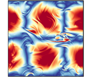



1. Introduction
Global stability analysis aims to provide a quantitative description of flow behaviour by analysing infinitesimal external disturbances superimposed on a complex base flow (Schmid Reference Schmid2007). The external disturbances may represent acoustic waves and vibration (Qin & Wu Reference Qin and Wu2016), surface roughness (Schrader, Brandt & Henningson Reference Schrader, Brandt and Henningson2009), free-stream turbulence (Schneider Reference Schneider2001; Joo & Durbin Reference Joo and Durbin2012; Brinkerhoff & Yaras Reference Brinkerhoff and Yaras2015), or neglected nonlinear terms in the governing equations (DelSole & Farrell Reference DelSole and Farrell1995). The disturbances may also be imposed on the initial condition.
Computational cost is one of the underlying challenges of performing global linear stability analysis (Kamal, Lakebrink & Colonius Reference Kamal, Lakebrink and Colonius2023). Many questions in global linear stability analysis require computing the response of the flow to high-dimensional infinitesimal disturbances. This means that the number of independent disturbances that need to be considered is typically very large and often proportional to the size of the state vector representing the flow in the discrete form. For example, building an input–output operator in a brute-force manner requires solving the inhomogeneous linearized system for the external excitation imposed on each state variable. Another example is determining the most amplified forcings and the most receptive states, which necessitates solving an optimization problem involving many expensive numerical simulations of the linearized Navier–Stokes equations. However, the computational cost varies greatly, depending on the complexity of the flow, whether the flow is homogeneous in any physical dimension, and whether the flow is steady, periodic, or arbitrarily time-dependent.
There are efficient numerical algorithms for performing global stability analysis when the base flow is steady. For steady-state base flows, modal global stability analysis requires solving large-scale eigenvalue problems. Krylov-based techniques (Edwards et al. Reference Edwards, Tuckerman, Friesner and Sorensen1994; Frantz, Loiseau & Robinet Reference Frantz, Loiseau and Robinet2023) have demonstrated excellent performance in extracting leading eigenmodes by projecting the linearized dynamics onto a lower-dimensional subspace, obtained through the orthonormalization of snapshots of the flow field. This technique has been used for the global stability analysis of a three-dimensional jet in crossflow (Bagheri et al. Reference Bagheri, Schlatter, Schmid and Henningson2009), where the base flow is forced to a steady-state solution using the selected frequency damping technique (Åkervik et al. Reference Åkervik, Brandt, Henningson, Hœpffner, Marxen and Schlatter2006). On the other hand, performing non-modal global stability analysis, even when the base flow is steady, requires computing a very large number of eigenmodes, especially for highly non-normal linearized operators. Although the fundamental solution operator formalism can be employed for stability analysis, computing this operator is computationally prohibitive for most practical flows, and is fraught with numerical challenges (Schmid & Henningson Reference Schmid and Henningson2001, § 6.4.2).
Similarly, computational algorithms based on resolvent analysis (Trefethen et al. Reference Trefethen, Trefethen, Reddy and Driscoll1993) have been employed successfully for computing the response to harmonic forcings when the base flow is steady (Schmidt et al. Reference Schmidt, Towne, Rigas, Colonius and Bres2018; Bae, Dawson & McKeon Reference Bae, Dawson and McKeon2020; Cook & Nichols Reference Cook and Nichols2022; Skene et al. Reference Skene, Yeh, Schmid and Taira2022). In resolvent analysis, the linear operator is obtained by linearizing the Navier–Stokes equations around the steady-state base flow or time-averaged mean flow (McKeon & Sharma Reference McKeon and Sharma2010). For many flows, the resolvent operator has fast-decaying singular values, which allows accurate low-rank approximation. This enables the development of numerous diagnostic and predictive tools, including the extraction of dominant coherent structures in turbulent flows (Abreu et al. Reference Abreu, Cavalieri, Schlatter, Vinuesa and Henningson2020), guiding the placement of sensors and actuators for flow control (Martini et al. Reference Martini, Jung, Cavalieri, Jordan and Towne2022; Jin, Illingworth & Sandberg Reference Jin, Illingworth and Sandberg2022), and reduced-order modelling of turbulent flows (McKeon Reference McKeon2017; Sun et al. Reference Sun, Liu, Cattafesta, Ukeiley and Taira2020).
The computational cost of constructing the resolvent operator and computing its low-rank approximation can be prohibitive for complex flows. If the flow has more than one non-homogeneous direction, then the explicit construction of the resolvent operator becomes costly or infeasible due to the storage and inversion of large matrices. Several methodologies have been proposed to address these issues, including the use of a modified randomized singular value decomposition (Ribeiro, Yeh & Taira Reference Ribeiro, Yeh and Taira2020) and methods based on time stepping (Monokrousos et al. Reference Monokrousos, Åkervik, Brandt and Henningson2010; Martini et al. Reference Martini, Rodríguez, Towne and Cavalieri2021) that involve the time integration of the linearized Navier–Stokes equation and its adjoint.
When the base flow is harmonically time-dependent, there are several approaches to perform stability analysis in a cost-effective manner. When the base flow is assumed to be time-invariant, the interactions across various frequencies cannot be computed. Floquet theory enables the stability analysis of linear systems that have periodic time dependence (Liu Reference Liu2003; Kern, Lupi & Henningson Reference Kern, Lupi and Henningson2024a). Resolvent analysis has also been extended recently to base flows with periodic time dependence (Padovan, Otto & Rowley Reference Padovan, Otto and Rowley2020; Padovan & Rowley Reference Padovan and Rowley2022), referred to as harmonic resolvent analysis. The computational cost of performing harmonic resolvent analysis can be significant as the number of considered frequencies increases. To this end, a methodology based on time stepping has recently been proposed to address this issue (Farghadan et al. Reference Farghadan, Jung, Bhagwat and Towne2024). To identify the optimal forcing and response modes that exhibit sparsity both spatially and temporally, a novel variant of resolvent analysis has been introduced (Lopez-Doriga et al. Reference Lopez-Doriga, Ballouz, Bae and Dawson2023). This method, termed space–time resolvent analysis, has been validated through application to statistically stationary channel flow and a time-periodic Stokes boundary layer.
The ability to simulate the evolution of disturbances for arbitrarily time-dependent flows in a cost-effective manner has significant implications for the stability analysis of complex flow problems. When the base flow is unsteady, the linearized operator continuously varies with time, and in general, the effect of this variation must be taken into account in the stability analysis. As mentioned above, while there are well-established and computationally efficient tools for performing linear stability analysis for problems with steady-state and time-periodic base flows, there are far fewer computationally efficient techniques for the stability analysis of unsteady flows (Schmid & Henningson Reference Schmid and Henningson2001, § 6.4.2). Although the fundamental solution operator formalism can be employed for stability analysis, computing this operator is computationally prohibitive for most practical flows.
An example application was studied recently by Kern et al. (Reference Kern, Negi, Hanifi and Henningson2024b), where linear stability analysis was performed for an aerofoil undergoing small-amplitude pitching motion. In this analysis, the base flow undergoes deformation due to a global instability mechanism, leading to secondary instability followed by a rapid breakdown to turbulence. Kern et al. (Reference Kern, Negi, Hanifi and Henningson2024b) investigate the effect of perturbation in the initial condition, which can be expressed as an initial-value problem for a homogeneous time-variant linear system. However, the effect of disturbance at the upstream boundary conditions, surface roughness, or neglected nonlinear terms can be formulated as a time-variant linear system subject to high-dimensional forcing. In these types of problems, the base flow variation with time is non-periodic and arbitrary, and it is not clear what instant of base flow should be chosen for using classical stability analysis methods such as eigenvalue decomposition. This is particularly important for flows with transient instabilities, where a steady base flow cannot be assumed, and using a time-averaged base flow results in a significant loss of information.
More broadly, the analysis of transient instabilities in high-dimensional dynamical systems such as turbulent flows demands cost-effective techniques to track the evolution of high-dimensional disturbance space. Transient instabilities are finite-time events, such as turbulent bursts or extreme events, whose response is markedly different from the high-dimensional attractor where the dynamical system spends most of its lifetime (Sapsis Reference Sapsis2021). Examples include turbulent bursts in laminar or turbulent flows (Avila et al. Reference Avila, Moxey, Lozar, Avila, Barkley and Hof2011; Cherubini & De Palma Reference Cherubini and De Palma2013; Farano et al. Reference Farano, Cherubini, Robinet and De Palma2017; Schmidt & Schmid Reference Schmidt and Schmid2019), the transition between a chaotic attractor and non-chaotic travelling waves (Modarres-Sadeghi et al. Reference Modarres-Sadeghi, Chasparis, Triantafyllou, Tognarelli and Beynet2011), and atmospheric blocking events (Davini et al. Reference Davini, Cagnazzo, Gualdi and Navarra2012).
Our objective is to develop a low-rank approximation of the solution operator for arbitrarily time-dependent base flows. This involves working with the arbitrarily time-dependent matrix obtained by linearizing the Navier–Stokes equations around the instantaneous base flow.
Our approach is to develop an input–output low-rank approximation based on forced optimally time-dependent decomposition (f-OTD) (Donello, Carpenter & Babaee Reference Donello, Carpenter and Babaee2022). The f-OTD is an extension of the OTD approximation (Babaee & Sapsis Reference Babaee and Sapsis2016), and it was originally developed by Donello et al. (Reference Donello, Carpenter and Babaee2022) for computing sensitivities in dynamical systems. The OTD and f-OTD have been utilized for many applications, including the computation of finite-time Lyapunov exponents (Babaee et al. Reference Babaee, Farazmand, Haller and Sapsis2017b), detection of the edge of chaos in dynamical systems (Beneitez et al. Reference Beneitez, Duguet, Schlatter and Henningson2020), prediction of bursting phenomena in high-dimensional dynamical systems (Farazmand & Sapsis Reference Farazmand and Sapsis2016), global transient stability analysis of a time-dependent base flow over an aerofoil (Kern et al. Reference Kern, Negi, Hanifi and Henningson2024b), control and linear instabilities (Blanchard & Sapsis Reference Blanchard and Sapsis2019; Kern et al. Reference Kern, Beneitez, Hanifi and Henningson2021), and skeletal kinetics (Nouri et al. Reference Nouri, Babaee, Givi, Chelliah and Livescu2022, Reference Nouri, Liu, Givi, Babaee and Livescu2024).
The OTD and f-OTD belong to a wider class of low-rank approximation methods used for matrix differential equations (MDEs) that rely on time-dependent bases (TDBs), where the solution of the MDE is evolved on a manifold of low-rank matrices. These TDB-based approximations originated in quantum chemistry and were utilized to solve high-dimensional Schrödinger equations (Beck et al. Reference Beck, Jäckle, Worth and Meyer2000). In Koch & Lubich (Reference Koch and Lubich2007), such techniques were presented for general MDEs under the name of dynamical low-rank approximation (DLRA). The dynamically orthogonal decomposition is another TDB-based method, tailored for solving stochastic partial differential equations (Sapsis & Lermusiaux Reference Sapsis and Lermusiaux2009). Both dynamically orthogonal and f-OTD techniques adopt a two-matrix factorization ( $\boldsymbol{\mathsf{V}} \approx \boldsymbol{\mathsf{U}} \boldsymbol{\mathsf{Y}}^{\mathrm {T}}$) for the full-rank matrix, while DLRA leverages a three-matrix factorization (
 $\boldsymbol{\mathsf{V}} \approx \boldsymbol{\mathsf{U}} \boldsymbol{\mathit{\Sigma}} \boldsymbol{\mathsf{Z}}^{\mathrm {T}}$). See § 2 for the notation used here. As demonstrated in Patil & Babaee (Reference Patil and Babaee2020, Theorem 2.2), two-matrix and three-matrix factorization methods are equivalent. The TDB-based approximations have been applied to various applications, such as turbulent combustion (Ramezanian, Nouri & Babaee Reference Ramezanian, Nouri and Babaee2021) and kinetics equations (Einkemmer & Lubich Reference Einkemmer and Lubich2018; Kusch & Stammer Reference Kusch and Stammer2023).
There are several other low-rank approximation techniques based on time-evolving subspaces. Spectral proper orthogonal decomposition (SPOD) extracts orthonormal time-dependent POD modes, with each mode oscillating at a single frequency (Towne, Schmidt & Colonius Reference Towne, Schmidt and Colonius2018). Recently, Frame & Towne (Reference Frame and Towne2023) proposed space–time POD where the modes vary arbitrarily with time. Both SPOD and space–time POD contrast with space-only POD, which is based on static subspaces. SPOD and space–time POD follow the same mathematical formalism as space-only POD, with the main difference being that the inner product of the SPOD and space–time modes is taken with respect to an integral over space and time.
The SPOD, space–time POD, and f-OTD low-rank approximations extract different types of correlations: SPOD and space–time POD extract spatiotemporal coherent structures, whereas f-OTD extracts instantaneous same-time correlations between different samples of the linearized dynamics. These different samples might be generated due to varying initial conditions or different forcings. Consequently, f-OTD modes are instantaneously orthonormal and vary arbitrarily with time, similar to space–time POD, rather than being time-periodic like SPOD. Another difference is that in SPOD and space–time POD, the bases are time-dependent, while the coefficients of the bases are constant; in f-OTD, both the bases and the coefficients are time-dependent. Additionally, f-OTD does not assume statistical stationarity, allowing it to be applied to flows that are not statistically stationary.
There is also an important difference between f-OTD and other data-driven low-rank approximation approaches: f-OTD is an equation-based low-rank approximation. Unlike SPOD and space–time POD, where modes are computed from data, evolution equations for the f-OTD subspace are derived from the linearized Navier–Stokes equations, and no offline data generation is required.
Perhaps it is more appropriate to compare SPOD and space–time POD to the dynamically orthogonal decomposition (Sapsis & Lermusiaux Reference Sapsis and Lermusiaux2009), which, in addition to being nonlinear and stochastic, shares all the attributes of f-OTD.
Recently, a continuous-time balanced truncation (CTBT) (Padovan & Rowley Reference Padovan and Rowley2024) has been proposed for time-periodic flows. This methodology extends the balanced POD – introduced by Rowley (Reference Rowley2012) for balanced truncation of time-invariant systems – to time-periodic flows. The approach presented by Padovan & Rowley (Reference Padovan and Rowley2024) results in a low-rank approximation based on time-evolving subspaces, where a time-continuous coordinate change and truncation are achieved by setting the time-dependent reachability and observability Gramians to be equal and diagonal. The CTBT low-rank approximation is closely related to harmonic resolvent analysis.
The similarity between f-OTD and CTBT is that the end product for both methodologies is a low-rank approximation based on time-evolving subspaces for forced time-dependent linear systems. However, the goals of these low-rank approximations are different. The CTBT aims to obtain a balanced truncation, which requires computing the Gramians. In contrast, f-OTD seeks to approximate the response of the forced linearized dynamics, and does not aim for a balanced truncation; thus computing Gramians is not needed in f-OTD. In that sense, f-OTD is more closely related to harmonic resolvent analysis than to CTBT. Another important distinction is that the f-OTD evolution equations are solved in the time domain rather than the frequency domain. Therefore, f-OTD can be utilized for forced linear systems that are arbitrarily time-dependent. In this paper, we consider one such problem where we use f-OTD to compute the response of linearized Navier–Stokes equations to a large number of impulses.
The structure of the paper is as follows. In § 2, we develop the f-OTD methodology for constructing low-rank solution operators for the forced linearized dynamics. In § 3, we demonstrate the capability of f-OTD on several examples, including a toy model, a one-dimensional Burgers equation, a two-dimensional temporally evolving jet, the chaotic Kolmogorov flow, and two-dimensional decaying isotropic turbulence. Finally, we discuss the main findings and provide concluding remarks in § 4.
2. Methodology
2.1. The MDEs for the operator evolution
In this subsection, we formulate the evolution of the disturbance due to different external forcings as an MDE. To this end, we consider the semi-discretized system where the governing equations are discretized in space. We consider a nonlinear dynamical system in the form
 \begin{equation} \dot{\boldsymbol{u}}= \boldsymbol{g}(\boldsymbol{u},t), \quad t \in I=[0,T], \end{equation}
where  $\boldsymbol {u}(t) \in \mathbb {R}^n$ represents the state of the dynamical system, and
 $\boldsymbol {g}(\boldsymbol {u},t) \in \mathbb {R}^n$ is a nonlinear function of the state. We consider the solution of (2.1) with the initial condition
 $\boldsymbol {u}(t=0)=\boldsymbol {u}_0$, and we denote the state of the trajectory at time
 $t$ by
 $\boldsymbol {u}(t)$. We consider the problem of the nonlinear dynamics prescribed by (2.1) subject to infinitesimal forcing. The resulting disturbance
 $\boldsymbol {v}$ satisfies the linear equation of variations:
 \begin{equation} \dot{\boldsymbol{v}}= \boldsymbol{\mathsf{L}}(\boldsymbol{u},t)\,\boldsymbol{v} + \boldsymbol{f}, \quad \boldsymbol{v}(0)=\boldsymbol{\mathsf{0}}, \end{equation}
where  $\boldsymbol {v}(t) \in \mathbb {R}^n$ is the state of the disturbance,
 $\boldsymbol{\mathsf{L}}(\boldsymbol {u},t) \in \mathbb {R}^{n\times n}$ is the matrix of the Jacobian of the vector field
 $\boldsymbol {g}(\boldsymbol {u},t)$, i.e.
 $\boldsymbol{\mathsf{L}}_{ij}=\partial \boldsymbol {g}_i/\partial \boldsymbol {u}_j$,
 $i,j=1, \dots, n$, and
 $\boldsymbol {f}(t) \in \mathbb {R}^n$ is the forcing vector. Equation (2.2) describes the effect of external forcing. The external forcing can represent free-stream turbulence, wall roughness or neglected terms, such as nonlinear terms (Schmid Reference Schmid2007). We consider cases where
 $\boldsymbol {f}$ belongs to a class of forcing:
 $\boldsymbol {f} \in \mathcal {S}$ with dimension
 $d$, i.e.
 $d=\mbox {dim}(\mathcal {S})$. Therefore, any forcing in the subset
 $\mathcal {S}$ can be determined with a set of
 $d$ coordinates and a set of basis vectors for
 $\mathcal {S}$:
 \begin{equation} \boldsymbol{f} = \sum_{j=1}^d y_j\,\boldsymbol{f}_{\!j}, \quad \forall \boldsymbol{f} \in \mathcal{S}, \end{equation}
where  $\boldsymbol {f}_{\!j} \in \mathbb {R}^n$ constitute a set of basis vectors for
 $\mathcal {S}$, i.e.
 $\mathcal {S}=\mbox {span}(\boldsymbol {f}_1, \boldsymbol {f}_2, \dots,\boldsymbol {f}_d)$, and
 $y_j \in \mathbb {R}$ are the coordinates. In the presented formulation, the forcing basis vectors do not need to be orthogonal; they need only to be independent. To investigate the response of (2.2) for any
 $\boldsymbol {f} \in \mathcal {S}$, we cast (2.2) as an MDE:
 \begin{equation} \dot{\boldsymbol{\mathsf{V}}}=
\boldsymbol{\mathsf{L}}(\boldsymbol{u},t)\,\boldsymbol{\mathsf{V}}
+ \boldsymbol{\mathsf{F}}, \quad \boldsymbol{\mathsf{V}}(0) = \boldsymbol{\mathsf{0}},
\end{equation}
where  $\boldsymbol{\mathsf{F}} =[\boldsymbol {f}_1, \boldsymbol {f}_2, \dots,\boldsymbol {f}_d] \in \mathbb {R}^{n\times d}$ is the matrix of forcing basis vectors, and
 $\boldsymbol{\mathsf{V}} =[\boldsymbol {v}_1, \boldsymbol {v}_2, \dots,\boldsymbol {v}_d] \in \mathbb {R}^{n\times d}$ is the matrix of corresponding response. The forcing matrix
 $\boldsymbol{\mathsf{F}}$ can be the actual forcing matrix as long as the forcings are independent. The dependent forcings need not be considered, as the response of the linear system to those dependent forcings can be obtained as a linear combination of the responses to the independent forcings.
We refer to (2.4) as the full-order model (FOM). Any column of  $\boldsymbol{\mathsf{V}}(t)$ contains the disturbances of all state variables for a single forcing, and each row of
 $\boldsymbol{\mathsf{V}}(t)$ contains the disturbances of a single state variable for all forcings. Each column of MDE (2.4) can be solved independently of other columns, while each row of MDE (2.4) is dependent on other rows, therefore each row cannot be solved independently.
The solution of the FOM given by (2.4) can be written as
 \begin{equation} \boldsymbol{\mathsf{V}}(t) = \int_0^t \boldsymbol{\mathit{\Phi}}(t,\tau)\,\boldsymbol{\mathsf{F}}(\tau) \,{\rm d}\tau, \end{equation}
where  $ \boldsymbol{\mathit{\Phi}} (t,\tau ) \in \mathbb {R}^{n \times n}$ is the fundamental solution operator, and its evolution is governed by the homogeneous disturbance evolution equation given by
 \begin{equation} \skew3\dot{ \boldsymbol{\mathit{\Phi}}}(t,\tau) = \boldsymbol{\mathsf{L}}(\boldsymbol{u},t)\, \boldsymbol{\mathit{\Phi}}(t,\tau), \quad \boldsymbol{\mathit{\Phi}}(\tau,\tau)= \boldsymbol{\mathsf{I}}, \quad t \geqslant 0, \end{equation}
where  $\boldsymbol{\mathsf{I}} \in \mathbb {R}^{n \times n}$ is the identity matrix. Since the MDE given by (2.4) is linear, the disturbance state for any
 $\boldsymbol {f} \in \mathcal {S}$ is given by
 \begin{equation} \boldsymbol{v}(t) = \left(\int_0^t \boldsymbol{\mathit{\Phi}}(t,\tau)\,\boldsymbol{\mathsf{F}}(\tau) \,{\rm d}\tau \right) \boldsymbol{y}, \end{equation}
where  $\boldsymbol {y} = [y_1,y_2,\dots,y_d]^{\mathrm {T}} \in \mathbb {R}^d$ is the coordinate of forcing
 $\boldsymbol {f}$ in the basis
 $\boldsymbol{\mathsf{F}} = [ \boldsymbol {f}_1, \boldsymbol {f}_2, \dots, \boldsymbol {f}_d]$. We define the operator
 $\boldsymbol {H}^t_{\mathcal {S}}$ as
 \begin{equation} \boldsymbol{H}^t_{\mathcal{S}}(\cdot) = \left(\int_0^t \boldsymbol{\mathit{\Phi}}(t,\tau)\,\boldsymbol{\mathsf{F}}(\tau) \,{\rm d}\tau \right) ({\cdot}), \end{equation}
for  $\boldsymbol {H}^t_{\mathcal {S}}(\cdot ): \mathbb {R}^d \rightarrow \mathbb {R}^{n}$. To calculate the response of any forcing
 $\boldsymbol {f} \in \mathcal {S}$ using the solution operator
 $\boldsymbol {H}^t_{\mathcal {S}}$, first
 $\boldsymbol {f}$ must be expressed in a forcing basis coordinate system according to (2.3). This is expressed as
 $\boldsymbol {f} = \boldsymbol{\mathsf{F}} \boldsymbol {y}$. The coordinate vector
 $\boldsymbol {y}$ is the input to the operator
 $\boldsymbol {H}^t_{\mathcal {S}}(\cdot )$. The output of the operator
 $\boldsymbol {H}^t_{\mathcal {S}}$ is the state of the disturbance, i.e.
 $\boldsymbol {v}(t) = \boldsymbol {H}^t_{\mathcal {S}}(\kern1pt\boldsymbol {y})$. The operator
 $\boldsymbol {H}^t_{\mathcal {S}}$ is an instantaneously linear operator that varies smoothly with time to adapt in response to changes in the state of the disturbances. In this view, the operator
 $\boldsymbol {H}^t_{\mathcal {S}}$ is a time-dependent matrix, and computing this operator is equivalent to computing
 $\boldsymbol{\mathsf{V}}(t)$. However, solving the FOM is computationally prohibitive, since both
 $n$ and
 $d$ are very large for most practical fluid dynamics applications.
2.2. On-the fly low-rank approximation with f-OTD
We present a novel application of low-rank approximation for an MDE based on time-dependent subspaces to approximate the solution of the FOM given by MDE (2.4). In particular, we formulate a low-rank approximation based on f-OTD. The f-OTD formulation seeks to approximate the solution of the FOM with a rank- $r$ matrix:
 \begin{equation} \boldsymbol{\mathsf{V}}(t) \approx \boldsymbol{\mathsf{U}}(t)\,\boldsymbol{\mathsf{Y}}(t)^{\mathrm{T}}, \end{equation}
where  $\boldsymbol{\mathsf{U}}(t) =[\boldsymbol {u}_1(t), \boldsymbol {u}_2(t), \dots, \boldsymbol {u}_r(t)] \in \mathbb {R}^{n \times r}$ is the matrix of the f-OTD modes, and
 $\boldsymbol{\mathsf{Y}}(t)=[\kern1pt\boldsymbol {y}_1(t), \boldsymbol {y}_2(t), \dots, \boldsymbol {y}_r(t)]\in \mathbb {R}^{d \times r}$ is the matrix of the f-OTD coefficient. The f-OTD modes are instantaneously orthonormal, i.e.
 ${\boldsymbol {u}_i(t)}^{\mathrm {T}} {\boldsymbol {u}_j(t)}= \delta _{ij}$, and they represent a low-rank time-dependent basis for the columns of matrix
 $\boldsymbol{\mathsf{V}}(t)$. The matrix
 $\boldsymbol{\mathsf{Y}}(t)$ represents a low-rank time-dependent basis for the rows of matrix
 $\boldsymbol{\mathsf{V}}(t)$. In the f-OTD formulation, the columns of
 $\boldsymbol{\mathsf{Y}}(t)$ are not orthogonal to each other.
Because f-OTD is a low-rank approximation, it cannot satisfy the FOM (2.4). Therefore, the f-OTD expansion satisfies the MDE (2.4) with a residual. To this end, a variational principle is utilized, which seeks to minimize this residual by optimally evolving the f-OTD components  ${ \boldsymbol{\mathsf{U}}(t)}$ and
 ${\boldsymbol{\mathsf{Y}}(t)}$ as
 \begin{equation} \mathcal{F}( \skew3\dot{\boldsymbol{\mathsf{U}}}, \skew3\dot{\boldsymbol{\mathsf{Y}}})= \left\| \frac{{\rm d}(\boldsymbol{\mathsf{U}}{\boldsymbol{\mathsf{Y}}}^{\mathrm{T}})}{{\rm d} t} -\boldsymbol{\mathsf{L}}\boldsymbol{\mathsf{U}} \boldsymbol{\mathsf{Y}}^{\mathrm{T}} -\boldsymbol{\mathsf{F}} \right\|^{2}_{F}, \end{equation}
where  $\|\cdot \|_F$ denotes the Frobenius norm. The dependence of matrices on
 $t$ and
 $\boldsymbol {u}$ is dropped for brevity. The above variational principle is subject to the orthonormality constraints of the spatial modes, i.e.
 ${\boldsymbol{\mathsf{U}}}^{\mathrm {T}}{\boldsymbol{\mathsf{U}}}=\boldsymbol{\mathsf{I}}$. The control parameters for the above function are
 $\skew3\dot {\boldsymbol{\mathsf{U}}}$ and
 $\skew3\dot {\boldsymbol{\mathsf{Y}}}$. The orthonormality constraints can be enforced via the Lagrange multipliers. To this end, we first take a time derivative of the orthonormality constraints:
 \begin{equation} \dot{\boldsymbol{u}}_i^{\mathrm{T}}{\boldsymbol{u}_j}+{\boldsymbol{u}_i}^{\mathrm{T}}{\dot{\boldsymbol{u}}_j}=0. \end{equation}
We denote  $\varPsi _{ij}: = {\boldsymbol {u}_i}^{\rm T}\dot {\boldsymbol {u}}_j$. It is clear from the above equation that
 $\boldsymbol{\mathit{\Psi}} =[\boldsymbol {\psi }_{ij}]\in \mathbb {R}^{ r \times r}$ is an arbitrary skew-symmetric matrix (
 $\boldsymbol{\mathit{\Psi}} ^{\mathrm {T}}=-\boldsymbol{\mathit{\Psi}} $). Incorporating the orthonormality condition into the variational principle leads to the unconstrained optimization problem
 \begin{equation} \boldsymbol{\mathcal{G}}(\skew3\dot{\boldsymbol{\mathsf{U}}}, \skew3\dot{\boldsymbol{\mathsf{Y}}},\boldsymbol{\mathit{\lambda}}) = \left\Vert \frac{{\rm d} (\boldsymbol{\mathsf{U}} \boldsymbol{\mathsf{Y}}^{\mathrm{T}})}{{\rm d} t} -\boldsymbol{\mathsf{L}}\boldsymbol{\mathsf{U}} \boldsymbol{\mathsf{Y}}^{\mathrm{T}} -\boldsymbol{\mathsf{F}} \right\Vert_F^{2}+ \sum_{i,j=1}^r \lambda_{ij} ( \boldsymbol{u}_i^{\mathrm{T}}\dot{\boldsymbol{u}}_j - \varPsi_{ij} ), \end{equation}
where  $\boldsymbol{\mathit{\lambda}} =[\lambda _{ij}]$,
 $i,j=1, \dots, r$, are Lagrange multipliers. The procedure for derivation of the optimality conditions is provided in Donello et al. (Reference Donello, Carpenter and Babaee2022). From the first-order optimality conditions of the unconstrained functional, the closed-form evolution equations for
 $\boldsymbol{\mathsf{U}}$ and
 $\boldsymbol{\mathsf{Y}}$ are derived:
 $$\begin{gather} \skew3\dot{\boldsymbol{\mathsf{U}}} = \boldsymbol{\mathsf{L}}\boldsymbol{\mathsf{U}}-\boldsymbol{\mathsf{U}}\boldsymbol{\mathsf{L}}_r+(\boldsymbol{\mathsf{F}}\boldsymbol{\mathsf{Y}}-\boldsymbol{\mathsf{U}}\boldsymbol{\mathsf{U}}^{\mathrm{T}}\boldsymbol{\mathsf{F}}\boldsymbol{\mathsf{Y}}){\boldsymbol{\mathsf{C}}}^{{-}1}, \quad\boldsymbol{\mathsf{U}}(t_0)=\boldsymbol{\mathsf{U}}_0, \end{gather}$$
 $$\begin{gather}\skew3\dot{\boldsymbol{\mathsf{Y}}}= \boldsymbol{\mathsf{Y}}\boldsymbol{\mathsf{L}}_r^{\mathrm{T}}+\boldsymbol{\mathsf{F}}^{\mathrm{T}}\boldsymbol{\mathsf{U}}, \quad \boldsymbol{\mathsf{Y}}(t_0)=\boldsymbol{\mathsf{Y}}_0, \end{gather}$$
where  $\boldsymbol{\mathsf{C}} = \boldsymbol{\mathsf{Y}}^{\mathrm {T}} \boldsymbol{\mathsf{Y}}\in \mathbb {R}^{ r \times r}$ is the reduced correlation matrix, and
 $\boldsymbol{\mathsf{L}}_r=\boldsymbol{\mathsf{U}}^{\mathrm {T}}{\boldsymbol{\mathsf{L}}\boldsymbol{\mathsf{U}}} \in \mathbb {R}^{ r \times r}$ is the reduced linear operator. We refer to f-OTD as an ‘on-the-fly’ low-rank approximation because it does not require the offline data generation commonly needed in data-driven reduced-order modelling. Instead, the matrix
 $\boldsymbol{\mathsf{V}}(t)$ is solved directly in its low-rank form, i.e. by evolving
 $\boldsymbol{\mathsf{U}}(t)$ and
 $\boldsymbol{\mathsf{Y}}(t)$. The f-OTD subspaces are initialized by first solving the FOM for
 $t_0 = \Delta t$, then computing the first
 $r$ singular vectors of
 $\boldsymbol{\mathsf{V}}(t_0) \approx \boldsymbol{\mathsf{U}}(t_0)\, \boldsymbol{\mathit{\Sigma}}(t_0)\,\boldsymbol{\mathsf{Z}}^{\mathrm {T}}(t_0)$, where
 $\boldsymbol{\mathsf{U}}(t_0) \in \mathbb {R}^{n\times r}$ is used as the initial condition for the f-OTD modes, and
 $\boldsymbol{\mathsf{Y}}(t_0) = \boldsymbol{\mathsf{Z}}(t_0)\, \boldsymbol{\mathit{\Sigma}}(t_0)$, where
 $ \boldsymbol{\mathit{\Sigma}}(t_0) \in \mathbb {R}^{r\times r}$ and
 $\boldsymbol{\mathsf{Z}}(t_0) \in \mathbb {R}^{d\times r}$ are the matrices of singular values and right singular vectors, respectively. In the case of very-large-scale dynamical systems, one can determine the initial conditions for the f-OTD matrices by a targeted sparse sampling of the FOM, which decreases the computational costs (Donello et al. Reference Donello, Palkar, Naderi, Del Rey Fernández and Babaee2023). This approach is based on the CUR low-rank approximation, where the approximation error can be made arbitrarily close to that of the same-rank singular value decomposition (SVD) low-rank approximation through oversampling.
One way to interpret the f-OTD evolution equations is as follows. Equation (2.13) determines the evolution of a time-dependent subspace in the phase space of the dynamics, and (2.14) is the reduced-order model obtained by the orthogonal projection of the FOM onto the time-evolving subspace  $\boldsymbol{\mathsf{U}}$. The above constrained minimization problem can be solved alternatively using Riemannian optimization, where the solution of MDE (2.4) is constrained on a rank-
 $r$ manifold. This will lead to the dynamical low-rank approximation for MDEs (Koch & Lubich Reference Koch and Lubich2007), which results in an equivalent low-rank approximation to the f-OTD formulation.
The evolution equations (2.13) and (2.14) are presented for generic dynamical systems. The f-OTD evolution equations for the incompressible Navier–Stokes equations are derived in Appendix A.
Note that  $\boldsymbol{\mathsf{L}}_r$ is time-dependent even when
 $\boldsymbol{\mathsf{L}}$ is not, due to the time dependence of
 $\boldsymbol{\mathsf{U}}$. The OTD equations can be derived from the f-OTD equations by setting
 $\boldsymbol{\mathsf{F}}$ to
 $\boldsymbol{\mathsf{0}}$. As demonstrated in Babaee & Sapsis (Reference Babaee and Sapsis2016), for a homogeneous linearized flow (where
 $\boldsymbol{\mathsf{F}}=\boldsymbol{\mathsf{0}}$) with a constant
 $\boldsymbol{\mathsf{L}}$, the subspace
 $\boldsymbol{\mathsf{U}}$ initially captures the non-normal growth in early disturbance evolution and eventually converges asymptotically to the rank-
 $r$ subspace spanned by the
 $r$ most unstable eigenvectors of
 $\boldsymbol{\mathsf{L}}$. Furthermore, as shown in Babaee et al. (Reference Babaee, Farazmand, Haller and Sapsis2017b), when
 $\boldsymbol{\mathsf{L}}$ is time-variant, the subspace
 $\boldsymbol{\mathsf{U}}$ converges exponentially to the eigenvectors of the Cauchy–Green strain tensor that corresponds to the most intense finite-time instabilities.
The rank of the f-OTD approximation is a hyperparameter, and increasing the rank improves the accuracy. In fact, for  $r=d$, the f-OTD equations recover the FOM. One heuristic approach to determine the rank is to find the smallest
 $r$ such that the ratio of the last resolved singular value to the Frobenius norm of the operator given by
 \begin{equation} \epsilon(t) = \frac{\sigma_r(t)}{\left(\sum_{i=1}^r \sigma_i^2(t)\right)^{1/2}} \end{equation}
is smaller than a threshold value. Ideally, f-OTD should be rank adaptive because, for a given accuracy criterion, the rank of the approximation needs to vary with time as the singular values of the solution matrix are time-dependent. This criterion has been used recently for a rank-adaptive TDB-based low-rank approximation for MDEs (Donello et al. Reference Donello, Palkar, Naderi, Del Rey Fernández and Babaee2023) and tensor differential equations (Ghahremani & Babaee Reference Ghahremani and Babaee2024). There are also other approaches for rank adaptivity for TDB-based low-rank approximations; see e.g. Dektor, Rodgers & Venturi (Reference Dektor, Rodgers and Venturi2021) and Ceruti, Kusch & Lubich (Reference Ceruti, Kusch and Lubich2022). All of the simulations performed in this paper are based on a fixed rank.
The f-OTD evolution equations become stiff when  $\boldsymbol{\mathsf{C}}$ is ill-conditioned as the inversion of this matrix appears in (2.13). A similar issue also occurs for DLRA and other equivalent TDB-based low-rank approximations. This issue has been the subject of research, and several different algorithms have been proposed that are robust in the presence of a near-singular or rank-deficient correlation matrix or singular value matrix; see e.g. Lubich & Oseledets (Reference Lubich and Oseledets2014), Ceruti & Lubich (Reference Ceruti and Lubich2021) and Donello et al. (Reference Donello, Palkar, Naderi, Del Rey Fernández and Babaee2023).
2.2.1. Computational cost
In the practical applications,  $n \sim O (10^9)$ and
 $d \sim O (10^3)\unicode{x2013} O (10^9)$, therefore solving the FOM is computationally prohibitive due to input–output and memory requirements as well as the floating point operations costs, which scale at least with
 $ O (nd)$. Equation (2.13) can be simplified to
 $\dot {\boldsymbol {u}}_i = \boldsymbol{\mathsf{L}}\boldsymbol {u}_i + \boldsymbol {r}_i$,
 $i=1,\dots, r$. The computational cost of evolving this equation is the same as solving
 $r$ samples of (2.2), i.e.
 $ O (rn)$. Equation (2.13) is a thin MDE, and the computation cost of solving this equation is
 $ O (rs)$. The right-hand side of the f-OTD evolution equations requires computing
 $\boldsymbol{\mathsf{U}}^{\mathrm {T}}\boldsymbol{\mathsf{F}}$ and
 $\boldsymbol{\mathsf{F}}\boldsymbol{\mathsf{Y}}$, which are both
 $ O (rdn)$. If the forcing is sparse, for example, when the forcing is localized at the boundaries, then this cost can become negligible. When
 $\boldsymbol{\mathsf{F}}$ is a dense matrix, the cost of computing these matrix–matrix multiplications can be reduced to
 $ O (r(n+d))$ using oblique projections and sparse sampling (Donello et al. Reference Donello, Palkar, Naderi, Del Rey Fernández and Babaee2023; Naderi & Babaee Reference Naderi and Babaee2023).
2.2.2. Mode ranking and the canonical form
The f-OTD subspace captures the most dominant perturbation subspace; however, the f-OTD modes and their coefficients are not ranked energetically. For example,  $\{\boldsymbol {u}_1,\boldsymbol {y}_1\}$ are not aligned with the first left and right singular vectors of the operator.
The f-OTD modes and the forcing coefficient can be ranked based on their significance after they are computed via (2.13) and (2.14). This is achieved through the eigen-decomposition of the reduced correlation matrix:  $\boldsymbol{\mathsf{C}}(t)\,\boldsymbol{\mathsf{R}}(t)=\boldsymbol{\mathsf{R}}(t)\,{\boldsymbol{\mathit{\Lambda}} }(t)$, where
 $\boldsymbol{\mathsf{C}}(t) = \boldsymbol{\mathsf{Y}}(t)^{\mathrm {T}} \boldsymbol{\mathsf{Y}}(t)$, and the matrix
 $\boldsymbol{\mathsf{R}}(t) \in \mathbb {R}^{r\times r}$ and
 ${\boldsymbol{\mathit{\Lambda}} }(t) = \mbox {diag}(\lambda _1(t), \dots, \lambda _r(t))$ are the eigenvector and eigenvalues of matrix
 $\boldsymbol{\mathsf{C}}(t)$, respectively. The eigenvalues of the correlation matrix are non-negative, i.e.
 $\lambda _i(t)\geqslant 0$, since
 $\boldsymbol{\mathsf{C}}$ is a positive symmetric matrix, and
 $\boldsymbol{\mathsf{R}}(t)$ is an orthonormal matrix. The eigenvalues of
 $\boldsymbol{\mathsf{C}}(t)$ can be ranked such that
 ${\lambda }_1(t) \geqslant {\lambda }_2(t) \geqslant \cdots \geqslant {\lambda }_r(t) \geqslant 0$. It is straightforward to show that
 $\sigma _i(t) = \lambda _i^{1/2}(t)$ are the singular values of the matrix
 $\boldsymbol{\mathsf{U}}(t) \boldsymbol{\mathsf{Y}}(t)^{\mathrm {T}}$. The f-OTD modes and modal coefficients can be rotated by disturbance energy (
 ${\sigma }_{i}^2$) in descending order as
 \begin{equation} \skew3\tilde{\boldsymbol{\mathsf{Y}}}(t) = \boldsymbol{\mathsf{Y}}(t)\,\boldsymbol{\mathsf{R}}(t)\,{ \boldsymbol{\mathit{\Sigma}}}^{{-}1}(t), \quad \skew3\tilde{\boldsymbol{\mathsf{U}}}(t)= \boldsymbol{\mathsf{U}}(t)\,\boldsymbol{\mathsf{R}}(t), \end{equation}
where  $ \boldsymbol{\mathit{\Sigma}}(t) =\mbox {diag}(\sigma _1(t), \dots, \sigma _r(t))$ is the matrix of singular values;
 $\skew3\tilde {\boldsymbol{\mathsf{Y}}}(t)$ and
 $\skew3\tilde {\boldsymbol{\mathsf{U}}}(t)$ are referred to as the bi-orthonormal form of the reduction, i.e.
 $\skew3\tilde {\boldsymbol{\mathsf{U}}}(t)^{\mathrm {T}}\skew3\tilde {\boldsymbol{\mathsf{U}}}(t) = \boldsymbol{\mathsf{I}}$ and
 $\skew3\tilde {\boldsymbol{\mathsf{Y}}}(t)^{\mathrm {T}}\skew3\tilde {\boldsymbol{\mathsf{Y}}}(t) = \boldsymbol{\mathsf{I}}$, where
 $\boldsymbol{\mathsf{I}} \in \mathbb {R}^{r\times r}$ is the identity matrix. We note that the bi-orthonormal forms {
 $\skew3\tilde {\boldsymbol{\mathsf{Y}}}(t), \boldsymbol{\mathit{\Sigma}}(t),\skew3\tilde {\boldsymbol{\mathsf{U}}}(t)$} and {
 $\boldsymbol{\mathsf{U}}(t) ,\boldsymbol{\mathsf{Y}}(t)$} are equivalent, i.e.
 $\skew3\tilde {\boldsymbol{\mathsf{U}}}(t)\, \boldsymbol{\mathit{\Sigma}}(t)\,{\skew3\tilde {\boldsymbol{\mathsf{Y}}}}(t)^{\mathrm {T}}={\boldsymbol{\mathsf{U}}(t)}$
 ${\boldsymbol{\mathsf{Y}}}(t)^{\mathrm {T}}$.
It is possible to write the evolution equations of the f-OTD modes directly in the energetically ranked form, i.e. the evolution equations for  ${\skew3\tilde {\boldsymbol{\mathsf{U}}},\skew3\tilde {\boldsymbol{\mathsf{Y}}}{ \boldsymbol{\mathit{\Sigma}}}}$ or
 ${\skew3\tilde {\boldsymbol{\mathsf{U}}}{ \boldsymbol{\mathit{\Sigma}}},\skew3\tilde {\boldsymbol{\mathsf{Y}}} }$. These evolution equations would result in subspaces equivalent to those obtained by solving (2.13) and (2.14). However, the evolution equations written in the energetically ranked form are not differentiable with time whenever there is a singular value crossing. The issue of singular value crossing has been extensively studied in the context of using the TDB for solving stochastic partial differential equations (Cheng, Hou & Zhang Reference Cheng, Hou and Zhang2013; Choi, Sapsis & Karniadakis Reference Choi, Sapsis and Karniadakis2014; Babaee et al. Reference Babaee, Choi, Sapsis and Karniadakis2017a; Patil & Babaee Reference Patil and Babaee2020). This issue manifests itself through the appearance of the term
 $1/(\sigma _i - \sigma _j)$ in the evolution equations of the TDB when written in the energetically ranked form. This can be understood intuitively: when the singular values cross, the more energetic mode before the crossing becomes the less energetic mode after the crossing. As a result, the more energetic mode, whose singular value is
 $\max \{\sigma _i,\sigma _j\}$, varies non-differentiably with time. These singularities do not occur for the f-OTD evolution equations, and as a result, the f-OTD modes vary smoothly with time.
2.2.3. Low-rank solution operator
In this subsubsection, we provide an operator interpretation of f-OTD. We consider the MDE (2.4) with a homogeneous initial condition, i.e.  $\boldsymbol{\mathsf{V}}(t=0) = \boldsymbol{\mathsf{0}}$. The low-rank operator for the MDE (2.4) is given by
 \begin{equation} \boldsymbol{H}^t_{\mathcal{S}}(\cdot) = \skew3\tilde{\boldsymbol{\mathsf{U}}}( t)\,{ \boldsymbol{\mathit{\Sigma}}}(t)\,\skew3\tilde{\boldsymbol{\mathsf{Y}}}(t)^{\mathrm{T}} (\cdot). \end{equation}
The inputs of the operator  $\boldsymbol {H}^t_{\mathcal {S}}: \mathbb {R}^d \rightarrow \mathbb {R}^{n}$ are the forcing coordinates
 $\boldsymbol {y} \in \mathbb {R}^d$, and the output of the operator is the state of the disturbance
 $\boldsymbol {v} \in \mathbb {R}^n$. The above operator constructed by f-OTD is an approximation to the operator given by (2.8). The above operator can be useful for a number of fluid dynamics problems; we highlight two of the key applications here.
(i) Surrogate modelling. The low-rank operator can serve as a rapid surrogate model to estimate responses to any forcing in
 $\mathcal {S}$. This is especially useful in receptivity analysis and uncertainty quantification. Once $\boldsymbol {H}^t_{\mathcal {S}}$ has been constructed, it allows for estimating responses to new forcings with minimal computational expense.
(ii) Optimal forcing. Operator
$\boldsymbol {H}^t_{\mathcal {S}}$ can be readily employed to find the most amplified forcing since it is factorized in the SVD form. The maximum disturbance energy is obtained by
(2.18)Moreover, the first right and left singular vectors of\begin{equation} G(t) =\max_{ \boldsymbol{y} \neq \boldsymbol{\mathsf{0}}} \dfrac{\|\boldsymbol{v}(t)\|^2_2}{\|\boldsymbol{y}\|^2_2} = \max_{ \boldsymbol{y} \neq \boldsymbol{\mathsf{0}}} \dfrac{\|\boldsymbol{H}^t_{\mathcal{S}}(\kern1pt\boldsymbol{y})\|^2_2}{\|\boldsymbol{y}\|^2_2} = \|\skew3\tilde{\boldsymbol{\mathsf{U}}}( t)\,{ \boldsymbol{\mathit{\Sigma}}}(t)\,\skew3\tilde{\boldsymbol{\mathsf{Y}}}(t)^{\mathrm{T}}\|^2_2= \sigma^2_1(t). \end{equation}$\boldsymbol {H}_{\mathcal {S}}^t$ are the optimal forcing and the state of the optimal disturbance, respectively. Specifically, the coefficient of the optimal forcing that achieves the highest amplification at a given time $t^*$ is represented by the vector $\boldsymbol {y}^* = \tilde {\boldsymbol {y}}_1(t^*)$. The corresponding optimal forcing is denoted as $\boldsymbol {f}^* = \boldsymbol{\mathsf{F}}\,\tilde {\boldsymbol {y}}_1(t^*)$, and the state of the optimal disturbance can be expressed as $\boldsymbol {v}^* = \sigma _1(t^*)\,\tilde {\boldsymbol {u}}_1(t^*)$.


3. Demonstration cases
In this section, we demonstrate the utility of f-OTD for various example problems.
3.1. Toy model
In the first example, we consider a three-dimensional nonlinear ordinary differential equation, which was analysed recently using harmonic resolvent analysis (Padovan et al. Reference Padovan, Otto and Rowley2020). The toy model is represented by the system of equations
 \begin{equation} \left.\begin{gathered} \dot{u}_1 = \mu u_1 - \gamma u_2 - \alpha u_1u_3 - \beta u_1u_2, \\ \dot{u}_2 = \gamma u_1 + \mu u_2 - \alpha u_2u_3 + \beta u_1^2, \\ \dot{u}_3 ={-}\alpha u_3 + \alpha(u_1^2 + u_2^2), \end{gathered}\right\} \end{equation}
where  $\mu =0.2$,
 $\gamma =1$,
 $\alpha =0.2$ and
 $\beta =0.2$. For the choice
 $\beta =0$, the above dynamical system corresponds to the reduced-order model of laminar flow around a cylinder (Noack et al. Reference Noack, Afanasiev, Morzynski, Tadmor and Thiele2003). Performing linearization of the above reduced-order model around the harmonically time-varying base state yields

where  $a_1=a_2=1$ and
 $a_3=0.01$. The matrix
 $\boldsymbol{\mathsf{L}} \in \mathbb {R}^{3\times 3}$, which represents the linearized system, is time-dependent due to its dependence on the current state of the system. The vector
 $\boldsymbol {v}_{i}$ is the response of the linearized system to the external forcing
 $\boldsymbol {f}_{i}(t)$, and
 $\boldsymbol{\mathsf{F}} =[\boldsymbol {f}_{1}(t), \boldsymbol {f}_{2}(t), \boldsymbol {f}_{3}(t)] \in \mathbb {R}^{3\times 3}$ is the matrix of external forcing, consisting of periodic signals at the frequency
 $\omega$. For the forcing frequency, we choose the limit cycle frequency, which is equal to
 $\omega =\sqrt {1-\beta ^2\mu /\alpha }$ (Padovan et al. Reference Padovan, Otto and Rowley2020).
To illustrate the utility of f-OTD, we choose a rank- $2$ f-OTD subspace (
 $r=2$) to approximate the response with a full rank (
 $d=3$). We integrate the nonlinear dynamical systems for
 $12 T$, where
 $T=2{\rm \pi} /\omega$ and
 $\omega = 0.98$. Here,
 $T$ and
 $\omega$ are the limit cycle period and frequency of the nonlinear dynamical system, respectively. Next, we solve the FOM with three different forcings for one time step to obtain
 $\boldsymbol{\mathsf{V}}(t_0)$, where
 $t_0 = \Delta t = T/2000$. We then perform the SVD on
 $\boldsymbol{\mathsf{V}}(t_0)$ to obtain the truncated rank-
 $2$ approximation of
 $\boldsymbol{\mathsf{V}}(t_0)$, i.e.
 $\boldsymbol{\mathsf{V}}(t_0) \approx \sigma _1(t_0)\,\tilde {\boldsymbol {u}}_1(t_0)\, \tilde {\boldsymbol {y}}_1(t_0)^{\mathrm {T}} + \sigma _2(t_0)\,\tilde {\boldsymbol {u}}_2(t_0)\, \tilde {\boldsymbol {y}}_2(t_0)^{\mathrm {T}}$. We then initialize the rank-
 $2$ f-OTD subspace as
 $\boldsymbol {u}_i(t_0) =\tilde {\boldsymbol {u}}_i(t_0)$ and
 $\boldsymbol {y}_i(t_0)=\sigma _i(t_0)\, \tilde {\boldsymbol {y}}_i(t_0)$ for
 $i=1,2$. For the time integration of the f-OTD equations, we use the explicit fourth-order Runge–Kutta method. The ground truth is also obtained by solving the FOM for
 $\boldsymbol{\mathsf{V}}(t) = [\boldsymbol {v}_1(t), \boldsymbol {v}_2(t),\boldsymbol {v}_3(t)]$.
The best time-dependent rank- $r$ approximation of the FOM solution is obtained by performing the SVD of
 $\boldsymbol{\mathsf{V}}(t)$ at each time step, and truncating at rank
 $r$. Comparing the singular values derived from f-OTD with those from the FOM serves as a valid metric for evaluating the performance of the f-OTD low-rank approximation. We first compute the fast Fourier transform of the singular values. We denote the spectra of
 $\sigma _i$ with
 $\hat {\sigma }_i$. The spectra of the two singular values of the rank-2 f-OTD and the first two singular values of the FOM are compared in figure 1. The spectra are computed after integrating the f-OTD for
 $15T$, i.e. fifteen cycles, which is sufficient for the f-OTD system to reach periodic behaviour, with the initial transient response having passed. The cross-frequency interaction between
 $\boldsymbol{\mathsf{L}}(t)$ and the monochromatic forcing is evident in the response. A good match between the spectra of f-OTD and the FOM is also observed.
Toy model, spectra of the singular values of f-OTD and FOM: (a) the first singular value; (b) the second singular value.

Now we investigate the relationship between the f-OTD low-rank approximation and the phase shift mode associated with the phase shift singularity of time-periodic linear systems. The phase shift mode exists in the linear time-periodic model of the toy problem, and it corresponds to the neutrally stable direction along the periodic orbit. The existence of this phase shift mode in time-periodic linear systems is trivial and may contaminate dynamically important amplification mechanisms. Therefore, we investigate the relationship between the f-OTD subspace and the direction associated with the phase shift mode.
The phase shift mode can be obtained by computing the eigenvector of the monodromy matrix associated with the eigenvalue 1. The monodromy matrix is a specific case of the fundamental solution matrix  $ \boldsymbol{\mathit{\Phi}} (t,\tau )$ presented in (2.6). In particular, the monodromy matrix is the fundamental solution matrix evaluated over one period
 $T$, i.e.
 $ \boldsymbol{\mathit{\Phi}} (t+T,t)$. To compute the phase shift mode, we perform the eigen-decomposition of
 $ \boldsymbol{\mathit{\Phi}} (t+T,t)$, where
 $ \boldsymbol{\mathit{\Phi}} (t+T,t)$ is the monodromy matrix obtained by solving (2.6) over one cycle. We denote the eigenvector of
 $ \boldsymbol{\mathit{\Phi}} (t+T,t)$ associated with the eigenvalue 1 as
 $\boldsymbol {v}_p(t)$.
We compute the angle between the f-OTD modes in the canonical form and  $\boldsymbol {v}_p(t)$. Assuming that
 $\boldsymbol {v}_p(t)$ has a unit norm, the angle between the phase shift mode and the f-OTD modes can be obtained as
 \begin{equation} \theta_i(t) = \cos^{{-}1}(\tilde{\boldsymbol{u}}_i^{\mathrm T}(t)\,\boldsymbol{v}_p(t) ). \end{equation}
The angles between the f-OTD modes and  $\boldsymbol {v}_p(t)$ are shown in figure 2(a). It is clear that none of the f-OTD modes is aligned with the phase shift mode; however, as time evolves, the angle between the first f-OTD mode (
 $\tilde {\boldsymbol {u}}_1$) and
 $\boldsymbol {v}_p(t)$ decreases, while the angle between the second f-OTD mode (
 $\tilde {\boldsymbol {u}}_2$) and
 $\boldsymbol {v}_p(t)$ increases. This behaviour is expected since
 $\tilde {\boldsymbol {u}}_2$ is orthogonal to
 $\tilde {\boldsymbol {u}}_1$.
Toy model: (a) angles between the phase shift mode and rank-2 f-OTD modes and rank-1 OTD mode; (b) projected limit cycle, phase shift vector and the canonical f-OTD vectors.

There is a closer connection between the phase shift mode and the OTD low-rank approximation, which corresponds to f-OTD low-rank approximation with no forcing, i.e.  $\boldsymbol{\mathsf{F}} = \boldsymbol{\mathsf{0}}$. First, we note that the phase shift mode is the least stable direction of the linearized dynamics of the toy model. As shown in Babaee et al. (Reference Babaee, Farazmand, Haller and Sapsis2017b), the OTD modes align themselves exponentially fast to the least stable subspace of the dynamical system. We perform a rank-1 OTD low-rank approximation of the linearized dynamics, and compute the angle between the OTD mode and
 $\boldsymbol {v}_p(t)$. This angle is also shown in figure 2(a). As expected, the OTD mode quickly aligns itself with
 $\boldsymbol {v}_p(t)$ as
 $\theta$ goes to zero.
The projected limit cycle, the phase shift vector and the f-OTD vectors at  $t=7T$ are shown in figure 2(b). The phase shift vector is tangent to the limit cycle, the first f-OTD vector makes a small angle with
 $\boldsymbol {v}_p$, and the second f-OTD vector is nearly orthogonal to
 $\boldsymbol {v}_p$.
Since the first f-OTD vector is not perfectly aligned with  $\boldsymbol {v}_p$, it still contains dynamically important information related to amplification mechanisms. Therefore, one can project the f-OTD modes onto the space spanned by the complement of the phase shift mode. Given that a rank-1 OTD captures the phase shift mode, a computationally efficient approach for high-dimensional systems is to solve a rank-1 OTD low-rank approximation alongside the f-OTD system, then project the f-OTD modes onto the complement of the OTD mode. This can be accomplished by computing
 \begin{equation} \boldsymbol{\mathsf{U}}^{{\perp}}_{\textrm{f-OTD}}(t) = \boldsymbol{\mathsf{U}}_{\textrm{f-OTD}}(t)-\boldsymbol{u}_{\textrm{OTD}}(t)\,\boldsymbol{u}_{\textrm{OTD}}(t)^{\mathrm T}\, \boldsymbol{\mathsf{U}}_{\textrm{f-OTD}}(t), \end{equation}
where  $\boldsymbol{\mathsf{U}}_{\textrm{f-OTD}}(t)$ is the f-OTD subspace,
 $\boldsymbol {u}_{\textrm{OTD}} \in \mathbb {R}^n$ is the rank-1 OTD approximation, and
 $\boldsymbol{\mathsf{U}}^{\perp }_{\textrm{f-OTD}}(t)$ is the projected f-OTD subspace onto the complement of rank-1 OTD mode.
3.2. Relationship between f-OTD and resolvent analysis
The purpose of this example is to demonstrate numerically a connection between the f-OTD low-rank approximation and resolvent analysis. To this end, we consider the linearized Burgers equation subject to harmonic forcing. We demonstrate numerically that the rank- $r$ f-OTD subspace asymptotically approximates the subspace obtained by the rank-
 $r$ SVD truncation of the resolvent operator. For this purpose, we consider the one-dimensional Burgers equation expressed as
 \begin{equation} {\partial{ {u_b}}\over{\partial t}} + \frac{1}{2}\,{\partial{u^2_b}\over{\partial x}} = \nu\,{\partial^2{u_b}\over{\partial x^2}} , \quad x\in[0,L], \end{equation}
where the base flow is denoted by  ${u_b}= {u_b}(x,t)$,
 $L=2{\rm \pi}$ is the length of the domain, and the viscosity is given by
 $\nu =0.02$. We consider the initial condition
 ${u_b}(x,0)=({1}/{s \sqrt {2{\rm \pi} }} )\exp ({-(x-{\rm \pi} )^2/2 s ^2})$ with
 $s=0.15$.
Since our goal is to compare f-OTD with resolvent analysis, we linearize the Burgers equation around a time-invariant state. Specifically, we consider the time-averaged solution of (3.5):
 \begin{equation} \bar{u}_b(x) = \frac{1}{T}\int_0^{T} u_b(x,t)\,{\rm d}t. \end{equation}
To investigate the amplification of disturbances around  $\bar {u}_b(x)$, we consider the linear evolution equation for the Burgers equation given by
 \begin{equation} {\partial{ v_{i}}\over{\partial t}}= L(v_i)+ f_{i}, \end{equation}
where  $L(v_i) := -{\partial (\bar {u}_b v_i)}/{\partial x} + \nu ({\partial ^2 v_i }/{\partial x^2})$ denotes the linearized Burgers operator. The discretized representation of the linear operator is a time-invariant matrix. The harmonic forcing is described by
 \begin{equation} f_{i}(x, t)=\boldsymbol{\delta}(x-x_i)\exp(j \omega t), \quad i=1,2, \dots, d, \end{equation}
where  $j=\sqrt{-1}$, and
 ${x_i}$ represent the grid points. The forcing basis functions
 $\boldsymbol {\delta }(x-x_i)$ are defined as
 $\boldsymbol {\delta }(x-x_i) =0$ when
 $x \neq x_i$, and
 $\boldsymbol {\delta }(x-x_i) =1$ when
 $x = x_i$. Here,
 $\omega =2{\rm \pi} /T$ signifies the frequency, with
 $T = 2$ being the period, and
 $d$ denotes the number of external excitations. We use
 $d=n$ independent forcings, implying that the number of forcings equals the dimension of the system. The parametrization of the forcing as given by (3.8) ensures that the f-OTD coefficient vectors (
 $\kern1pt\boldsymbol {y}_i \in \mathbb {R}^n$) are defined on the same grid as the state vectors.
For the spatial discretization of the Burgers equation, the FOM, and the f-OTD equations, we use the Fourier spectral method with  $n=256$ Fourier modes. For the temporal discretization, we use the exponential time-differencing fourth-order Runge–Kutta method (Kassam & Trefethen Reference Kassam and Trefethen2005) with time step
 $\Delta t= 0.01$. We first solve the Burgers equation for one period (
 $T$). The mean state (
 $\bar {u}_b(x)$) is computed as the mean of
 $u_b(x,t)$ during this period. We solve the f-OTD equations using
 $\bar {u}_b(x)$ in the linearized operator. The f-OTD modes and coefficients are initialized by selecting the first
 $r$ dominant modes from the FOM solution at the final time step of the period.
We now explain how f-OTD can be compared to resolvent analysis. While the f-OTD equations are solved in the temporal domain, the resolvent analysis is performed in the frequency domain. To facilitate this comparison, we convert the f-OTD reconstructed solution ( $\boldsymbol{\mathsf{U}}(t)\,\boldsymbol{\mathsf{Y}}(t)^{\mathrm {T}}$) into the frequency domain using the fast Fourier transform. The fast Fourier transform is applied to each column of the
 $\boldsymbol{\mathsf{U}}(t)\,\boldsymbol{\mathsf{Y}}(t)^{\mathrm {T}}$ matrix.
The f-OTD low-rank approximation is solved as an initial-value problem capturing both the transient evolution of the disturbance and its asymptotic behaviour. As resolvent analysis captures the asymptotic behaviour, we focus on comparing the f-OTD response after long-time integration. To this end, we solve the f-OTD evolution equations for 16 units of time. This duration ensures that the f-OTD reconstructed solution achieves a statically converged state. Due to the absence of significant separation between the resolvent singular values, a relatively large f-OTD rank  $r=80$ is chosen. Therefore,
 $\boldsymbol{\mathsf{U}}$ and
 $\boldsymbol{\mathsf{Y}}$ are both of size
 $256 \times 80$, and
 $\boldsymbol {H}^t_{\mathcal {S}} = \boldsymbol{\mathsf{U}}(t)\,\boldsymbol{\mathsf{Y}}(t)^{\mathrm {T}}$ is a rank-80 approximation of the instantaneous solution operator. We then apply the fast Fourier transform to each column of
 $\boldsymbol {H}^t_{\mathcal {S}}$ to obtain a frequency domain solution operator, which is denoted as
 $\hat {\boldsymbol {H}}_{\mathcal {S}}(\omega )$. The temporal solution of the f-OTD asymptotically converged to a harmonic behaviour with the same frequency as
 $\omega$. We use the f-OTD solution during the last two periods to compute
 $\hat {\boldsymbol {H}}_{\mathcal {S}}(\omega )$.
The 15 leading singular values of  $\hat {\boldsymbol {H}}_{\mathcal {S}}(\omega )$ are compared against those obtained from resolvent analysis in figure 3(a). The results indicate that the asymptotic solution of the f-OTD subspace and the resolvent analysis agree well with one another. In figure 3(b), we compare the first dominant response and forcing modes obtained from resolvent analysis and the f-OTD approximation. In particular, the first left and right singular vectors of the resolvent operator and those obtained from f-OTD are shown. Excellent agreement between these singular vectors is observed. This example demonstrates numerically the connection between f-OTD and resolvent analysis. One might be able to rigorously establish a connection between f-OTD and resolvent analysis by analysing the f-OTD response to a harmonically forced time-invariant linear system – similar to the results that showed the asymptotic convergence of OTD modes (
 $\boldsymbol{\mathsf{F}}=\boldsymbol{\mathsf{0}}$) to the least unstable subspace of
 $\boldsymbol{\mathsf{L}}$ (Babaee & Sapsis Reference Babaee and Sapsis2016, Theorem 2.3). However, such mathematical development is beyond the scope of the current study.
Resolvent analysis (RA) and f-OTD for the Burgers equation. (a) Comparison of the first  $15$ dominant singular values of the resolvent operator with the asymptotic solution of f-OTD. (b) The first dominant response and forcing mode from the resolvent operator and f-OTD.

3.3. Temporally evolving jet
In this subsection, we demonstrate the capability of f-OTD for a transient flow with an arbitrary time-dependent base flow. We consider the temporally mixing layer, which is a classic example of transient disturbance growth and has been studied extensively; see e.g. Broze & Hussain (Reference Broze and Hussain1994) and Arratia, Caulfield & Chomaz (Reference Arratia, Caulfield and Chomaz2013). The transient evolution of the mixing layer exhibits time-varying dynamics, transient non-normal growth, and vortex pairing, all of which make it a compelling test case for the f-OTD demonstration. A schematic representation of the mixing layer can be seen in figure 4. It is important to note that throughout the period under consideration ( $0 \leqslant t \leqslant 30$), the base flow exhibits arbitrary time dependence. Additionally, the flow experiences a transition due to vortex pairing.
Schematic of the temporally evolving jet, showing the evolution of the base flow at different time instances ( $t_1=12$,
 $t_2 =15$,
 $t_3 =18$,
 $t_4=21$).

In the following, we use the f-OTD reconstructed input–output operator to find the worst-case disturbance, i.e. the most amplified disturbance. When the base flow is arbitrarily time-dependent, finding the most amplified disturbance requires solving an optimization problem, typically using a gradient-based optimization algorithm. Computing the gradient necessitates solving the adjoint equation, which must be done backwards in time and requires storing the time-resolved nonlinear state. In general, adjoint equations are costly to solve for large-scale problems due to the input–output cost of storing and reading the nonlinear state from disk. Additionally, the iterations of gradient-based optimization algorithms have a sequential workflow due to the dependency of each iteration on the previous one, making them quite costly.
3.3.1. Problem set-up
The evolution of the base flow is governed by the incompressible Navier–Stokes equations. The f-OTD evolution equations are presented in Appendix A. Equations (A1)–(A2) are subject to periodic boundary conditions in the  $x$ and
 $y$ directions. The computational domain extends from
 $x = 0$ to
 $x = L$, and from
 $y = 0$ to
 $y = H$, with both
 $L$ and
 $H$ being equal to 1. For enhanced visualization, the contour plots are displayed over a domain with length
 $2L$. The initial velocity is given by
 $\boldsymbol {u}_b(x,y,t_0) = \bar {\boldsymbol {u}}(y) + \boldsymbol {u}'(x,y)$, where
 $\bar {\boldsymbol {u}}(y)$ is the initial velocity profile, and
 $\boldsymbol {u}'(x,y)$ is a divergence-free fluctuation velocity field to trigger the transition from laminar to an unsteady flow. The norm of
 $\boldsymbol {u}'(x,y)$ is four orders smaller than the norm of
 $\bar {\boldsymbol {u}}(y)$. The velocity profile
 $\bar {\boldsymbol {u}}(y) = [\bar u_x(y), 0]^{\mathrm {T}}$ is defined as
 \begin{equation} \bar{u}_x(y) = \frac{u_{m}}{2}\left(\tanh\left(\frac{y-y_s}{\delta}\right) - \tanh\left(\frac{y-y_e}{\delta}\right) - 1 \right), \end{equation}
where  $\delta = 0.01$,
 $y_s = 0.45$,
 $y_e = 0.55$ and
 $u_{m} = 1$ are used in this study. The jet is centred in the middle. We consider a Reynolds number given by
 $Re = u_{m}H/\nu = 10^{4}$. The forced linearized Navier–Stokes equations that govern the evolution of disturbances due to external forcing, as well as the f-OTD equations for the incompressible Navier–Stokes equations, are given in Appendix A. Equations (A3)–(A4) constitute the FOM in this demonstration.
The two-dimensional incompressible Navier–Stokes equations, the FOM, and the evolution equations for f-OTD are solved using the Fourier spectral method, employing  $N_x = N_y = 2^7$ Fourier modes in each direction. For the time integration, we utilize a fourth-order Runge–Kutta scheme with time step
 $\Delta t = 3.125 \times 10^{-3}$. To initialize the time-varying base flow, we integrate the incompressible Navier–Stokes equations for 25 time units. Subsequently, the solution from the final time step is taken as the initial condition for the base flow. Figure 4 depicts the base flow evolution at various time instances.
3.3.2. Harmonic forcing
To generate the localized forcing, we introduce the expressions
 $$\begin{gather} \tilde{f}_{x}(x,y)= \frac{I(y)}{k_x } \cos(2{\rm \pi} k_x x)\sin(2{\rm \pi} k_y y), \end{gather}$$
 $$\begin{gather}\tilde{f}_{y}(x,y)={-}\dfrac{I(y)}{k_y } \sin(2{\rm \pi} k_x x)\cos(2{\rm \pi} k_y y), \end{gather}$$
where  $I(y) = \tanh ({(y-y_s)}/{\delta }) - \tanh ({(y-y_e)}/{\delta })$ serves as the indicator function that localizes the forcing within the region defined by
 $y_s \leqslant y \leqslant y_e$, and different forcings are generated by varying the wavenumbers
 $k_x$ and
 $k_y$. The vector field
 $\tilde {\boldsymbol {f}}= [\tilde {f}_{x},\tilde {f}_{y}]^{\mathrm {T}}$ is not divergence-free due to the multiplication of
 $I(y)$ by each component. We map this vector field to a divergence-free vector field using the projection function
 $\phi$, which is obtained by solving
 $\nabla ^2 \phi = \boldsymbol {\nabla }\boldsymbol {\cdot }\tilde {\boldsymbol {f}}$ and updating the vector field using the relations
 $$\begin{gather} f_{x}(x,y,t)=c \left(\tilde{f}_x(x,y) - \frac{\partial \phi}{\partial x}\right)\sin(\omega t), \end{gather}$$
 $$\begin{gather}f_{y}(x,y,t)=c \left(\tilde{f}_y(x,y) - \frac{\partial \phi}{\partial y}\right)\sin(\omega t). \end{gather}$$
It is easy to verify that the vector field  $(f_x,f_y)$ is divergence-free. Here, the coefficient
 $c$ determines the energy spectrum of each force component and is given by
 $c=1/(k_x+k_y)$. We consider a total of
 $d=144$ external excitations by varying the wavenumbers
 $k_x=[1,2, \dots, 12]$ and
 $k_y=[1,2, \dots, 12]$. We consider the tensor product of these sets, and generate
 $d=144$ forcings. The temporal forcing frequency is denoted by
 $\omega$, and for all the forcings considered in this problem, we set
 $\omega = 0.37$. This excitation frequency is identified as one of the dominant frequencies in the nonlinear base flow.
The space–time discretization of the f-OTD equation is identical to that of the FOM. To initialize the f-OTD modes and modal coefficients, we solve the FOM for one time step for all  $d=144$ forcings. We construct a matrix of the FOM solution, wherein the matrix has
 $2N_x N_y = 2^{15}$ rows, corresponding to the total number of grid points times two for the two components of velocity, and
 $d=144$ columns, with each column representing the response to each forcing. We then perform SVD on this matrix, and set the rank-
 $r$ SVD-truncated matrix as the initial condition for the f-OTD subspace. For very large dynamical systems, the initial condition for the f-OTD matrices can be computed through a targeted sparse sampling of the FOM to reduce computational costs (Donello et al. Reference Donello, Palkar, Naderi, Del Rey Fernández and Babaee2023).
Figure 5 displays a comparison of normalized singular values between the FOM and f-OTD. To compute the normalized singular values, we divide the instantaneous singular value from f-OTD and the FOM by the total sum of the FOM singular values at each time instance. We solve the f-OTD equations with rank  $r=8$, and figure 5 illustrates that the largest singular values are approximated accurately by f-OTD.
Temporally evolving jet: comparison of the dominant normalized singular values obtained from the FOM and f-OTD.

The reason why the f-OTD singular values do not perfectly match those of the FOM is that f-OTD provides an approximation of the best low-rank solution, which is obtained by performing SVD on the FOM solution. Since f-OTD is a reduced-order model, errors from reduced-order modelling accumulate over time (i.e. memory error), causing the singular values to deviate from those of the FOM.
The dimensionality of this system varies over time, as observed by the clustering of singular values at the beginning ( $0 \leqslant t \leqslant 5$) where many modes are required to approximate the FOM. As the flow evolves, two time-dependent f-OTD modes become dominant – growing by two to three orders of magnitude larger than the other modes. The dominance of the first two singular values suggests that the response to various forcings can be approximated accurately with a low-rank approximation based on TDBs.
Figure 6 demonstrates the efficacy of f-OTD reduction in reconstructing the disturbance field when there is a strong cross-frequency interaction between the forcing frequency and the base flow. We examine two distinct excitations,  $v_1$ and
 $v_{13}$, corresponding to wavenumbers
 $(k_x, k_y) = (1, 1)$ and
 $(k_x, k_y) = (2, 1)$, respectively. The figure presents a comparison of the temporal evolution of the f-OTD reconstructed response and the FOM at two different locations,
 $A$ and
 $B$, with coordinates
 $(x_A, y_A) = (0.39, 0.59)$ and
 $(x_B, y_B) = (0.10, 0.12)$. The disturbance exhibits transitional multi-frequency behaviour, attributable to the cross-frequency interactions between the harmonic forcing frequency and the arbitrarily time-dependent base flow. It is observed that f-OTD low-rank approximation captures this evolution accurately.
Temporally evolving jet: comparison of the temporal evolution of the perturbation velocity at two probe locations,  $(x_A,y_A) = (0.39, 0.59)$ and
 $(x_B,y_B) = (0.10, 0.12)$.

Figure 7 displays snapshots of the first four dominant f-OTD spatial modes at different time instances, sorted by their singular values from the most dominant to the least dominant modes. The dashed lines show the contours of vorticity for the base flow. The first two modes are associated with the dominant singular values  $\sigma _1(t)$ and
 $\sigma _2(t)$, and exhibit similar structures. The dominant modes capture the largest structures, while the lower modes extract finer structures. It is also evident that the f-OTD modes evolve instantaneously with the base flow.
Temporally evolving jet: the first four dominant left singular vectors of the f-OTD low-rank solution operator at different times (dashed lines show the base flow's vorticity). The f-OTD modes are energetically ranked in descending order.

Figure 8 shows the time evolution of the orthonormalized modal coefficients  $\skew3\tilde {\boldsymbol{\mathsf{Y}}}(t)^{\mathrm {T}}$. Each row approximates a right singular vector of the solution operator, while each column represents the contribution of each excitation to different modes. As time progresses, the modal coefficients evolve, capturing the time-dependent contribution of different forces to the f-OTD low-rank subspace. For example, at
 $t_1=2$, the first row (
 $\tilde {\boldsymbol {y}}_1^{\mathrm {T}}$) shows that among all
 $144$ excitations,
 $\boldsymbol {f}_1$ and
 $\boldsymbol {f}_{13}$, associated with wavenumbers
 $(k_x,k_y)=(1,1)$ and
 $(2,1)$, respectively, have the most significant contributions. However, the third row (
 $\tilde {\boldsymbol {y}}_3^{\mathrm {T}}$), associated with
 $\sigma _3$, demonstrates the dominant contributions of
 $\boldsymbol {f}_2$ and
 $\boldsymbol {f}_{14}$. The modal coefficients contain rich insights into the excitations and can be exploited for physical or dynamical understanding.
Temporally evolving jet: the first eight dominant right singular vectors ( $\skew3\tilde {\boldsymbol{\mathsf{Y}}}^{\mathrm {T}}(t)$) of the f-OTD low-rank solution operator at different times.

We utilize the low-rank approximation of the solution operator based on f-OTD to determine the optimal forcing without incurring additional computational costs. In particular, we seek to identify the forcing  $\boldsymbol {f} \in \mathcal {S}$ whose response achieves maximum amplification at
 $t = t^*$ among all forcings in
 $\mathcal {S}$. As demonstrated in § 2.2.3, the optimal forcing is obtained from
 $\boldsymbol {f}^* = \boldsymbol{\mathsf{F}}\,\tilde {\boldsymbol {y}}_1(t^*)$, leading to maximal amplification at the designated time
 $t^*$. To obtain the optimal perturbation vector, we solved (2.2) with the forcing
 $\boldsymbol {f}=\boldsymbol{\mathsf{F}}\,\tilde {\boldsymbol {y}}_1(t^*)$. To underscore the significance of the optimal forcing vector
 $\tilde {\boldsymbol {y}}_1(t^*)$, we solved (2.2) for a random excitation
 $\boldsymbol {f}_{Rand} = \boldsymbol{\mathsf{F}}\,\boldsymbol {y}_{Rand}$, where
 $\|\boldsymbol {y}_{Rand}\|=1$. In figure 9(a), we compare the evolution of disturbance energy resulting from these two different external forcings. The grey line represents the maximum possible amplification
 $G_{max}(t)=\sigma _1^2(t)$, which signifies the maximal energy that any
 $\boldsymbol {f} \in \mathcal {S}$ can achieve; it can be regarded as the envelope of perturbation energy for all
 $\boldsymbol {f} = \boldsymbol{\mathsf{F}}\boldsymbol {y}$, where
 $\|\boldsymbol {y}\|=1$. It is evident that the response to the optimal forcing, shown by the dashed black line, reaches the envelope (
 $\sigma ^2_{1}$) at
 $t^*$, shown by a blue circle, after which its energy decays. In contrast, the energy of the random excitation experiences growth but remains roughly one to two orders of magnitude smaller than the maximum possible amplification.
Temporally evolving jet: comparison between optimal forcing and a random forcing within the forcing space. At time  $t^*=18.75$, the magnitudes of the optimal and random forcings with their corresponding responses are displayed.

To demonstrate the capability of f-OTD as a rapid surrogate model, we obtain state disturbance due to the optimal forcing using the operator
 \begin{equation} \boldsymbol{v}^*(t)=\boldsymbol{H}^t_{\mathcal{S}}(\tilde{\boldsymbol{y}}_1(t^*)) = \skew3\tilde{\boldsymbol{\mathsf{U}}}( t)\,{ \boldsymbol{\mathit{\Sigma}}}(t)\,\skew3\tilde{\boldsymbol{\mathsf{Y}}}(t)^{\mathrm{T}} \,(\tilde{\boldsymbol{y}}_1(t^*) ). \end{equation}
Note that  $\tilde {\boldsymbol {y}}_1(t^*)$ is not a time-dependent vector. The energy of this solution is shown with cross symbols, which matches well with the disturbance obtained by solving (2.2), which is the ground truth in this setting.
Figures 9(b)–9(e) illustrate the structures of these excitations and their corresponding responses at time  $t^*$. The
 $x$-component of the response to the forcing is shown in (figures 9c) and (9e). The optimal forcing in figure 9(b) exhibits a significant presence in the shear layer and is influenced by lower wavenumbers. In figures 9(c) and 9(e), we observe that the flow responses share similar structures; however, they have completely different magnitudes. The fact that the disturbance resulting from the random forcing has a shape similar to that of the optimal disturbance is because
 $\boldsymbol {y}_{Rand}$ has a small projection onto the optimal
 $\tilde {\boldsymbol {y}}_1(t^*)$. Given that this direction in the forcing space grows significantly faster than other directions, its response ultimately dominates the shape of the disturbance.
3.4. Two-dimensional chaotic Kolmogorov flow
The purpose of this demonstration is to show the performance of f-OTD in computing the response of a chaotic flow subject to high-dimensional external excitations. In particular, we consider a chaotic flow that exhibits a short-lived intermittent phenomenon.
We consider the two-dimensional chaotic Kolmogorov flow (Platt, Sirovich & Fitzmaurice Reference Platt, Sirovich and Fitzmaurice2024) governed by the forced incompressible Navier–Stokes equations
 \begin{equation} \frac{\partial \boldsymbol{u}_b}{\partial t} + (\boldsymbol{u}_b \boldsymbol{\cdot}\boldsymbol{\nabla}) \boldsymbol{u}_b ={-} \boldsymbol{\nabla} p_b + \frac{1}{Re}\,\nabla^2 \boldsymbol{u}_b + \boldsymbol{f}_{\!b}, \quad \boldsymbol{\nabla}\boldsymbol{\cdot}\boldsymbol{u}_b = 0, \end{equation}
where  $\boldsymbol {u}_b(x,y,t) =[u_b(x,y,t),v_b(x,y,t)]^{\mathrm {T}}$ is the time-dependent base flow, and
 $\boldsymbol {f}_b(y) = \sin (n y)\,\boldsymbol {e}_1$, with
 $\boldsymbol {e}_1 = [1, 0]^{\mathrm {T}}$. The flow is considered in the physical domain
 $(x,y) \in [0, 2{\rm \pi} ]\times [0, 2{\rm \pi} ]$, with periodic boundary conditions in both
 $x$ and
 $y$. The Kolmogorov flow has a laminar solution
 \begin{equation} \boldsymbol{u}_b(y) = \frac{Re}{n^2} \sin (n y)\,\boldsymbol{e}_1. \end{equation}
The above laminar profile is stable for  $n=1$ and any Reynolds number. For
 $n>1$ and a sufficiently large Reynolds number, the above laminar solution is unstable (Platt et al. Reference Platt, Sirovich and Fitzmaurice2024) .
The Kolmogorov flow has applications in magnetohydrodynamics, where it can be reproduced using appropriate magnetic and electric fields. For a review of the Kolmogorov flow and its applications, see Fylladitakis (Reference Fylladitakis2018).
We consider  $n=4$ and
 $Re=40$, which result in an unstable flow. Under these parameters, the flow is chaotic and exhibits a strange attractor. Moreover, for these parameters, the Kolmogorov flow exhibits intermittent dynamics, which manifests itself as short-lived burst of energy dissipation. The energy dissipation is defined as
 \begin{equation} D(t) = \frac{1}{Re\,L^2 }\int_0^{L} \int_0^{L} |\omega(x,y,t) |^2 \,{{\rm d}\kern0.07em x} \,{{\rm d}y}, \end{equation}
where  $\omega (x,y,t)$ is the vorticity, and
 $L=2{\rm \pi}$ is the length of the domain in each dimension. Also, the energy input is defined as
 \begin{equation} I(t) = \frac{1}{L^2 }\int_0^{L} \int_0^{L} \boldsymbol{u}_b(x,y,t)\boldsymbol{\cdot}\boldsymbol{f}_{\!b}(y)\, {{\rm d}\kern0.07em x}\, {{\rm d} y}. \end{equation}
In figure 10(a),  $D(t)$ versus
 $I(t)$ is shown. This figure portrays the chaotic attractor as well as the excursion from the attractor.
The Kolmogorov flow: (a) energy input versus energy dissipation; (b) evolution of the energy dissipation  $D$; and (c) largest eigenvalue
 $\lambda ^S_1$ of the symmetric part for the reduced linear matrix
 $\boldsymbol {S}_r$ for
 $d=16\,384$.

The bursting phenomenon was studied by Farazmand & Sapsis (Reference Farazmand and Sapsis2016), where the OTD low-rank approximation is used to build indicators for these extreme events. We also consider the same parameters as Farazmand & Sapsis (Reference Farazmand and Sapsis2016), i.e.  $n=4$ and
 $Re=40$. In this work, we investigate the effect of external forcing disturbance as opposed to the initial condition perturbations considered by Farazmand & Sapsis (Reference Farazmand and Sapsis2016).
We use f-OTD for the numerical simulation of the Kolmogorov flow subject to high-dimensional external disturbances. In particular, we consider divergence-free forcing disturbances in the form
 \begin{equation} f_{x}(x,y)= \frac{c}{k_x}\cos(k_x x) \sin(k_y y), \quad f_{y}(x,y)={-} \dfrac{c}{k_y} \sin(k_x x)\cos(k_y y), \end{equation}
where  $c =1/(k_x^2+k_y^2)$ is the forcing spectrum. Here,
 $k_x$ and
 $k_y$ are the wavenumbers ranging from
 $1$ to
 $p$, i.e.
 $k_x=[1,2,\dots, p]$ and
 $k_y=[1,2,\dots, p]$. Therefore, the total number of external excitations considered is
 $d=p^2$. The external forcing defined above should be viewed as infinitesimal disturbances to the base flow
 \begin{equation} \frac{\partial \boldsymbol{u}'_b}{\partial t} + (\boldsymbol{u}'_b \boldsymbol{\cdot}\boldsymbol{\nabla}) \boldsymbol{u}'_b ={-} \boldsymbol{\nabla} p'_b + \frac{1}{Re}\,\nabla^2 \boldsymbol{u}'_b + \boldsymbol{f}_{\!b} + \epsilon \boldsymbol{f}, \end{equation}
where  $\boldsymbol {f} = [f_x, f_y]^{\mathrm {T}}$ is the external disturbance vector, and
 $\boldsymbol {u}'_b$ and
 $p'_b$ are the perturbed velocity and pressure fields, respectively. Therefore, the disturbance field is
 $\boldsymbol {v} = (\boldsymbol {u}'_b - \boldsymbol {u}_b)/\epsilon$ as
 $\epsilon \rightarrow 0$. The evolution of
 $\boldsymbol {v}$ is governed by the forced linearized Navier–Stokes equations (A3) and (A4) presented in Appendix A. Different forcings
 $\boldsymbol {f}_i$, for
 $i=1,2,\dots, d$ are obtained by considering all combinations of wavenumbers
 $k_x$ and
 $k_y$ in their respective ranges, which generates the disturbance
 $\boldsymbol {v}_i$. The base flow driving force (
 $\boldsymbol {f_b}$) does not appear in the linearized Navier–Stokes equations because
 $\boldsymbol {f_b}$ is not a function of the state variables and therefore is unperturbed.
We solve the base flow and the f-OTD equations using the same numerical methods as in the previous example. We consider a grid of size  $128 \times 128$, and
 $\Delta t = 0.004$.
We consider two cases,  $p=10$ and
 $p=128$, which results in
 $d=10^2 = 100$ and
 $d=128^2=16\,384$, respectively. The dimension of the space spanned by the forcing in the case
 $d=128^2$ is equal to the size of the grid points. The case with
 $p=10$ is considered for verification purposes, for which we solve the FOM. For the case
 $p=128$, solving the FOM is too costly because it requires solving 16 384 linearized Navier–Stokes equations. For this case, we perform only the f-OTD simulations.
We first integrate the base flow until it reaches the attractor. To this end, we initialize the base flow with the steady-state profile given by (3.16), superimposed with small divergence-free perturbations. For the chosen parameters, the base flow is unstable and becomes chaotic and arbitrarily time-dependent. We integrate the flow until  $t_0=210$, after which an intermittent phenomenon occurs, as is evident in the dissipation shown in figure 10(b). We then solve the FOM for one time step, and compute the SVD of the FOM and truncate at rank
 $r$ to initialize the f-OTD low-rank matrices.
The f-OTD reconstruction can be used to compute the response ratio for any of the forces. For this problem, the forcing is not time-dependent, and the response ratio is the ratio of the norm of the disturbance to the norm of the corresponding forcing:
 \begin{equation} R_i(t) = \frac{\| \boldsymbol{v}_i(x,y,t)\|}{\|\kern1pt\boldsymbol{f}_i(x,y)\|}, \quad i=1,2, \dots, d. \end{equation}
An advantage of computing the response ratio is that it removes the effect of the forcing spectrum; in other words, the forcings that are attenuated in the spectrum are restored to their original magnitudes. If the forcing spectrum is not used, then the singular values will cluster near the initial evolution, requiring a large rank. Therefore,  $R_i(t)$ is an objective metric to assess the performance of f-OTD and also an important quantity for analysing how the flow responds to individual forces.
The norm of  $\boldsymbol {v}_i$ using f-OTD does not require explicitly forming
 $\boldsymbol {v}_i$, and it can be computed using the low-rank approximation as
 \begin{align} \|\boldsymbol{v}_i \|^2 = \left\| \sum_{m=1}^r y_{im} \boldsymbol{u}_m \right\|^2 &= \left\langle \sum_{m=1}^r y_{im} \boldsymbol{u}_m,\sum_{m'=1}^r y_{im'} \boldsymbol{u}_{m'} \right\rangle\nonumber\\ &= \sum_{m=1}^r \sum_{m'=1}^r y_{im} y_{im'}\left\langle \boldsymbol{u}_m , \boldsymbol{u}_{m'} \right\rangle\nonumber\\ &= \sum_{m=1}^r \sum_{m'=1}^r y_{im} y_{im'}\delta_{m m'} = \sum_{m=1}^r y^2_{im}, \end{align}
where  $y_{im}$ is the
 $(i,m)$ entry of the f-OTD coefficient matrix, i.e.
 $y_{im} = \boldsymbol{\mathsf{Y}}_{(i,m)}$. In the above derivation, we have made use of the orthonormality properties of the f-OTD modes. Therefore,
 $\| \boldsymbol {v}_i \|$ is equal to the second norm of
 $i$th row of the
 ${\boldsymbol{\mathsf{Y}}}$ matrix, which can be computed at a negligible computational cost.
The response ratios for the case  $d=100$ and the f-OTD rank
 $r=20$ at three different time instants are shown in figure 11. These response ratios for 100 forcings are shown in the
 $k_x$–
 $k_y$ plane. The corresponding quantities are also calculated from the FOM. It is clear that the flow is much more responsive to the forces with lower wavenumbers. Moreover, comparing the f-OTD results with the FOM shows that the f-OTD approximation tends to be more accurate for the most excited forces. This is not surprising, as f-OTD seeks to capture the most amplified subspace, which in this problem is dominated by response to forces with lower wavenumbers.
The Kolmogorov flow: response ratio for  $d=100$ and
 $r=20$.

Now we consider the case with  $d=16\,384$. Solving the FOM for this case is cost-prohibitive. Therefore, we perform the f-OTD low-rank approximation for only three ranks,
 $r=10$,
 $15$ and 20, to demonstrate convergence. We show how the f-OTD low-rank approximation can be used to extract quantities that describe the intermittent events. To this end, we compute the eigenvalues of the symmetric part of
 $\boldsymbol{\mathsf{L}}_r$. The matrix
 $\boldsymbol{\mathsf{L}}_r$ is the reduced linear operator that is obtained by projecting the full-dimensional instantaneous linear operator onto the f-OTD subspace, i.e.
 $\boldsymbol{\mathsf{L}}_r = \boldsymbol{\mathsf{U}}^\textrm {T} \boldsymbol{\mathsf{LU}} \in \mathbb {R}^{r\times r}$. The symmetric part of
 $\boldsymbol{\mathsf{L}}_r$ is given by
 \begin{equation} \boldsymbol{\mathsf{S}}_r = \frac{\boldsymbol{\mathsf{L}}_r+\boldsymbol{\mathsf{L}}_r^{\mathrm{T}}}{2}. \end{equation}
The eigenvalues of  $\boldsymbol{\mathsf{S}}_r$ are real and can be sorted such that
 $\lambda ^S_1 \geqslant \lambda ^S_2 \geqslant \cdots \geqslant \lambda ^S_r$, and
 $\lambda ^S_1$ represents the maximum instantaneous growth rate within the f-OTD subspace (Farrell & Ioannou Reference Farrell and Ioannou1996). In figure 10(b), the energy dissipation is depicted, which shows an intermittent event during the time interval
 $t \in [210, 260]$. In figure 10(c),
 $\lambda ^S_1(t)$ for three f-OTD ranks are shown. We observe that the intermittent event causes a significant increase in
 $\lambda ^S_1$. Moreover, as
 $r$ increases,
 $\lambda ^S_1$ converges to an upper envelope.
The singular values for  $r=10$,
 $15$ and
 $20$ are shown in figure 12. It is clear that the leading singular values have converged, and there is a larger discrepancy between the singular values of
 $r=10$,
 $15$ and 20 for modes with lower energy. The leading singular values grow exponentially with time due to the chaotic nature of the dynamics. There is also a large gap between the leading singular values, indicating that the resulting MDE is instantaneously low-rank.
The Kolmogorov flow: convergence study for singular values evolution from f-OTD for different reduction sizes ( $r=20$,
 $15$ and
 $10$) for
 $d=16\,384$.

3.5. Two-dimensional decaying isotropic turbulence
In this subsection, we present the application of f-OTD in low-rank approximation of the response of the linearized Navier–Stokes equation to a large number of impulses, which has utility in flow control and in particular balanced truncation reduced-order models (Moore Reference Moore1981; Lall, Marsden & Glavaški Reference Lall, Marsden and Glavaški1999; Rowley Reference Rowley2012).
The post-transient response of the linearized Navier–Stokes equations and their adjoint to an impulse is widely used in control to estimate the Gramians, as solving the time-dependent Lyapunov equation in the time domain is prohibitive for large-scale dynamical systems. When the base flow is steady-state, it is possible to compute the Gramians cost-effectively. For periodic base flows, Padovan & Rowley (Reference Padovan and Rowley2024) proposed an effective approach to compute the frequential Gramians by solving them in the frequency domain. However, for arbitrarily time-dependent base flows, computing the Gramians requires determining the response of the direct and adjoint linearized Navier–Stokes equations to a very large number of impulses, which is computationally taxing.
In this demonstration, we show that the f-OTD low-rank approximation can reduce the computational cost of solving this problem. Specifically, we illustrate the computational advantages of formulating the response to a large number of impulses as an MDE. We demonstrate numerically that the resulting MDE is instantaneously low-rank. These low-rank properties are then exploited using f-OTD by approximating the solution of the MDE on the manifold of low-rank matrices.
For the demonstration, we consider two-dimensional decaying turbulent flow. This flow is chosen due to its complex dynamics, highly unsteady and time-dependent base flows, and chaotic nature (Jiménez Reference Jiménez2020). The simulations are conducted using the same numerical methods as those explained in § 3.3. The computational domain is a square with length  $L = 2{\rm \pi}$, discretized with a
 $512 \times 512$ grid. We use the time step
 $\Delta t =0.001$ for temporal advancement, and
 $Re=10\,000$. The flow fields are initialized using the Taylor–Green vortex (Vuorinen & Keskinen Reference Vuorinen and Keskinen2016).
For this problem, we employ an external forcing in space that acts impulsively at the initial time. We define the external forcing as
 \begin{equation} f_{x}(x,y,t)= \frac{c}{k_x }\cos(k_x x) \sin(k_y y)\,g(t), \quad f_{y}(x,y,t)={-} \dfrac{c}{k_y} \sin(k_x x)\cos(k_y y)\, g(t), \end{equation}
where  $g(t)$ is the impulse function, defined as
 \begin{equation} g(t) = \begin{cases} 1 & \text{if } t = t_0, \\ 0 & \text{if } t > t_0, \end{cases} \end{equation}
where  $t_0=\Delta t$.
The forcing spectrum is the same as that used for the Kolmogorov flow. In this study, the wavenumbers  $k_x$ and
 $k_y$ varied from
 $1$ to
 $32$. We considered a total of
 $d=1024$ external excitations, and employed a subspace size
 $r=30$ for the f-OTD reduction, which yielded satisfactory results. For this analysis, we conducted only f-OTD simulations. The f-OTD was initialized by computing the FOM for a single time step, after which the initial conditions for the f-OTD were assigned by using the first
 $r$ rank from the SVD of the FOM solution.
To demonstrate the convergence of the f-OTD modes, we compare the leading singular values from two different subspace sizes,  $r=20$ and
 $30$. As illustrated in figure 13, the singular values match well with each other, indicating that
 $r=20$ is sufficiently large. There is also a large gap between the singular values, especially between the first singular values and the rest, indicating that this problem is instantaneously low-rank.
Two-dimensional decaying isotropic turbulence: singular value of f-OTD with  $r = 20$ and
 $30$ of post-transient response matrix to
 $d=1024$ impulses.

The computational cost of solving the f-OTD equations is approximately equal to solving  $r$ forced linearized Navier–Stokes equations; see § 2.2.1 for more details. Therefore, the computational savings offered by f-OTD, in terms of floating point operations, memory and input–output, is approximately equal to the factor
 $d/r$.
Figure 14 presents the temporal evolution of the first three dominant f-OTD modes in canonical form, as well as the base flow, at five time instances. The base flow is visualized by the values of the vorticity  $|\boldsymbol {\nabla } \times \boldsymbol {u}_b|$, and the f-OTD modes, in the canonical form, are visualized by the f-OTD vector at each grid point, i.e.
 $|\tilde {\boldsymbol {u}}_i(x,y,t)| = (\tilde {u}_{x_i}(x,y,t)^2+\tilde {u}_{y_i}(x,y,t)^2)^{1/2}$, where
 $\tilde {u}_{x_i}$ and
 $\tilde {u}_{y_i}$ are the
 $x$- and
 $y$-components of
 $\tilde {\boldsymbol {u}}_i(x,y,t)$. The results show a rapid realignment of the initial f-OTD subspace to the dynamically dominant perturbation subspace in the early stages of the evolution (
 $0< t<0.2$). During this period, although the base flow has barely changed, the f-OTD subspace evolves very quickly. As time progresses, the effect of the base flow evolution on the f-OTD modes becomes evident, resulting in rich and complex modes that evolve with the base flow. The response to the impulse becomes highly localized over time, as manifested by the strong presence of the f-OTD modes in small regions of the flow.
Two-dimensional decaying isotropic turbulence: evolution of the first three dominant f-OTD modes and the base flow for low-rank approximation of the post-transient response to  $d=1024$ impulses. The base flow is visualized by the magnitude of vorticity
 $|\boldsymbol {\nabla } \times \boldsymbol {u}_b|$, and the modes are visualized by the magnitude of the f-OTD vector at each grid point,
 $|\tilde {\boldsymbol {u}}_i| = (\tilde {u}_{x_i}^2+\tilde {u}_{y_i}^2)^{1/2}$.

4. Conclusion
Analysis of linear disturbance growth due to external forcing is crucial for flow stability, control, and uncertainty quantification. However, when the base flow is arbitrarily time-dependent, the computational tools that are effective for analysing steady-state base flows become either inadequate or too computationally prohibitive to use. To this end, we present a methodology to build low-rank solution operators for the linear evolution of disturbance for problems with unsteady base flows. The solution operator is a time-dependent matrix whose evolution equation is governed by forced linearized dynamics. The formulation is based on the forced optimally time-dependent decomposition (f-OTD), in which the solution operator is approximated by the multiplication of two skinny time-dependent matrices. Using a variational principle, evolution equations for these two matrices are derived. The f-OTD low-rank approximation is equivalent to the dynamical low-rank approximation and similarly constrains the solution of the matrix differential equation to a manifold of low-rank matrices.
We demonstrate the utility of the developed methodology through several case studies. These demonstrations show how the methodology can identify the optimal forcing and employ the operator as an effective surrogate model. We also show the connection between the presented methodology and the resolvent analysis. In particular, we show numerically that when it is applied to the steady-state mean flow, the presented low-rank approximation converges asymptotically to that of the resolvent analysis.
Two mathematical developments are of interest for future studies: (i) rigorously proving the connection between the asymptotic behaviour of f-OTD and resolvent analysis; (ii) developing a rank-adaptive f-OTD methodology that determines the rank of the low-rank approximation at each time instant, based on the accuracy requirements of the solution operator.
Acknowledgements
The authors are grateful to the reviewers for their comments, which led to several improvements. In particular, we thank Reviewer 1 for highlighting the potential contamination of the f-OTD subspace due to the phase shift singularity, which prompted our investigation into this issue, as discussed in the toy model results. This research was supported in part by the University of Pittsburgh Center for Research Computing through the resources provided.
Funding
We gratefully acknowledge support funding from Transformational Tools and Technology (TTT), NASA grant no. 80NSSC22M0282, and the National Science Foundation (NSF), USA, under the grant CBET2042918.
Declaration of interests
The authors report no conflict of interest.
Appendix A. The f-OTD derivation for the incompressible Navier–Stokes equations
In this appendix, we present the f-OTD evolution equations for the incompressible Navier–Stokes equations. The incompressible Navier–Stokes equations govern the evolution of the base flow as
 $$\begin{gather} \frac{\partial \boldsymbol{u}_b}{\partial t} + (\boldsymbol{u}_b \boldsymbol{\cdot}\boldsymbol{\nabla}) \boldsymbol{u}_b = \boldsymbol{\nabla} p_b + \frac{1}{Re}\,\nabla^2 \boldsymbol{u}_b, \end{gather}$$
 $$\begin{gather}\boldsymbol{\nabla}\boldsymbol{\cdot}{\boldsymbol{u}_b} = 0, \end{gather}$$
where  ${\boldsymbol {u}_b}(x,y,t)$ is the velocity vector field with components
 ${\boldsymbol {u}_b}(x,y,t) = [u_b(x,y,t), v_b(x,y,t)]^{\mathrm {T}}$, and
 ${p}_b(x,y,t)$ is the pressure field. The evolution equation for disturbance
 $\boldsymbol {v}_i(x,y,t)$ is given by
 $$\begin{gather} \frac{\partial \boldsymbol{v}_i}{\partial t} = \mathcal{L}_{NS}( \boldsymbol{v}_i) -\boldsymbol{\nabla} p_i + \boldsymbol{f}_i, \end{gather}$$
 $$\begin{gather}\boldsymbol{\nabla}\boldsymbol{\cdot} { \boldsymbol{v}_i} = 0, \end{gather}$$
where  $\mathcal {L}_{NS}(\cdot )$ is the linearized Navier–Stokes operator given by
 \begin{equation} \mathcal{L}_{NS}(\boldsymbol{v}_i) ={-} (\boldsymbol{u}_b \boldsymbol{\cdot}\boldsymbol{\nabla}) \boldsymbol{v}_i - (\boldsymbol{v}_i \boldsymbol{\cdot}\boldsymbol{\nabla}) \boldsymbol{u}_b+\frac{1}{Re}\, \nabla^2 \boldsymbol{v}_i, \quad i=1,2,\dots, d, \end{equation}
and  $\boldsymbol {f}_i(x,y,t) = [f_{x_i}(x,y,t),f_{y_i}(x,y,t)]^{\mathrm {T}}$ is the external forcing. The matrix
 ${\boldsymbol{L}}$ and vector
 $\boldsymbol {f}_i$ in the f-OTD evolution equations are the discrete representations of
 $\mathcal {L}_{NS}$ and
 $\boldsymbol {f}_{\!i}(x,y,t)$, respectively. For the incompressible Navier–Stokes equations, each f-OTD mode is a vector field, i.e.
 $\boldsymbol {u}_i = [u_{x_i}, u_{y_i}]^{\mathrm {T}}$, for
 $i=1, \ldots, r$. The f-OTD modes are orthonormal with respect to the inner product
 \begin{equation} \left\langle \boldsymbol{u}_i,\boldsymbol{u}_j \right\rangle = \iint (u_{x_i} u_{x_j} + u_{y_i} u_{y_j}) \, {{\rm d}\kern0.07em x} \, {{\rm d}y}, \quad \|\boldsymbol{u} \| = \left\langle \boldsymbol{u},\boldsymbol{u} \right\rangle^{1/2}. \end{equation}
The induced norm is also defined above. Moreover, the f-OTD vector field must be divergence-free to ensure that any f-OTD reconstructed field is also divergence-free. Therefore,  $\boldsymbol {\nabla }\boldsymbol {\cdot } \boldsymbol {u}_i =0$. To enforce the divergence-free condition, we use the projection method. Below, we explain the steps for the time integration for the f-OTD equations for an explicit Euler scheme.
(i) Solve (2.13), in which
$\boldsymbol{\mathsf{L}}$ is the discrete representation of $\mathcal {L}_{NS}$ operator given by (A5):
(A7)where the solution at time step\begin{equation} \skew3\hat{\boldsymbol{\mathsf{U}}}^{k+1} = \boldsymbol{\mathsf{U}}^{k} + \Delta t \left(\boldsymbol{\mathsf{L}}^k\boldsymbol{\mathsf{U}}^k-\boldsymbol{\mathsf{U}}^k\boldsymbol{\mathsf{L}}^k_r+ (\boldsymbol{\mathsf{F}}^k\boldsymbol{\mathsf{Y}}^k-\boldsymbol{\mathsf{U}}^k\boldsymbol{\mathsf{U}}^{k^{\mathrm{T}}}\boldsymbol{\mathsf{F}}^k \boldsymbol{\mathsf{Y}}^k){\boldsymbol{\mathsf{C}}}^{k^{{-}1}} \right), \end{equation}$k$ is denoted with a superscript $k$, and $\Delta t$ is the time advancement magnitude. For an efficient implementation of this step, it is important to note that the matrix $\boldsymbol{\mathsf{L}}$ does not need to be formed explicitly; rather, what is required is the action of $\boldsymbol{\mathsf{L}}$ on vector fields.(ii) Note that the pressure gradient is not included in the linearized operator, and as a result, the columns of
$\skew3\hat {\boldsymbol{\mathsf{U}}}^{k+1}$, denoted by $\hat {\boldsymbol {u}}_i^{k+1}$, are not divergence-free. In this step, we use the projection method to project $\hat {\boldsymbol {u}}_i^{k+1}$ onto a divergence-free vector field:
(A8)where\begin{equation} \left.\begin{gathered} \boldsymbol{\mathsf{D}} \boldsymbol{\mathsf{G}} \boldsymbol{\phi}^{k+1}_i = \boldsymbol{\mathsf{D}} \hat{\boldsymbol{u}}_i^{k+1}, \quad i=1,2, \dots, r,\\ \boldsymbol{u}_i^{k+1} = \hat{\boldsymbol{u}}_i^{k+1} - \boldsymbol{\mathsf{G}} \boldsymbol{\phi}^{k+1}_i, \end{gathered}\right\} \end{equation}$\boldsymbol{\mathsf{D}} \in \mathbb {R}^{n \times 2n }$ and $\boldsymbol{\mathsf{G}} \in \mathbb {R}^{2n \times n}$ are the discrete representations of the gradient and divergence operators, respectively.(iii) In the final step, we advance the evolution equation for the f-OTD coefficients using the divergence-free f-OTD modes:
(A9)\begin{equation} \boldsymbol{\mathsf{Y}}^{k+1} = \boldsymbol{\mathsf{Y}}^k + \Delta t \left( \boldsymbol{\mathsf{Y}}^k\boldsymbol{\mathsf{L}}_r^{k^{\mathrm{T}}}+\boldsymbol{\mathsf{F}}^{k^{\mathrm{T}}}\boldsymbol{\mathsf{U}}^k \right). \end{equation}


We use the fourth-order Runge–Kutta scheme for the time integration of the f-OTD equations. Time advancement of every stage of the Runge–Kutta scheme is analogous to the explicit Euler scheme explained above.


 Open access

