Coated transmission-line method

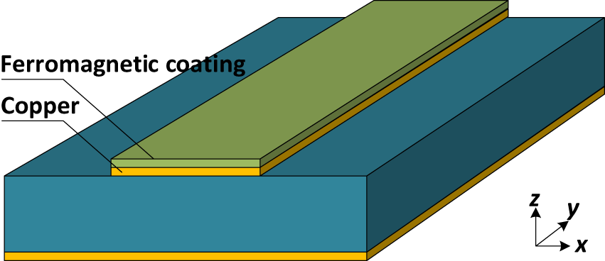
The fact that a microstrip line can be analytically modeled with transmission line theory makes it an ideal measurement platform. The microwave ferromagnetic thin film can be coated or plated onto the surface of the upper conductor of a microstrip line, as shown in Figure 1. A dual-carrier signal is fed into the microstrip line. Because the permeability of the ferromagnetic material depends on the magnetic field, i.e., its constitutive relation is nonlinear, the signals propagating along the microstrip line generate nonlinear signal components. Since the nonlinear signals carry the information of the materials’ nonlinear parameters, we can extract them by establishing the relationship between these nonlinear signals and the nonlinear parameters. In the following, transmission line theory is employed to derive the relationship between the PIM of a ferromagnetic-material-coated microstrip line and its third-order permeability.

Figure 1.

Schematic diagram of a ferromagnetic-material-coated microstrip line.

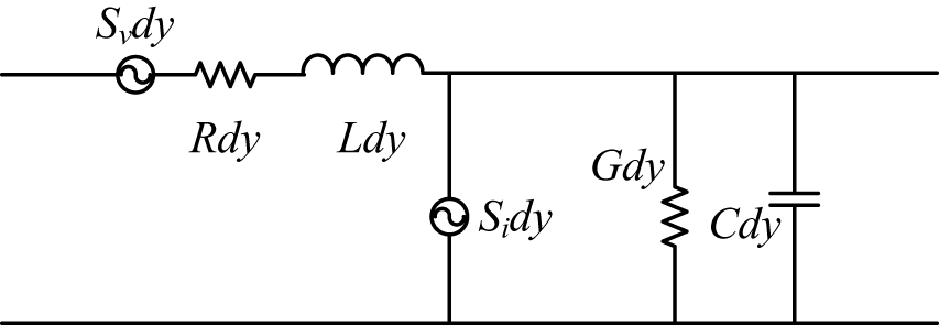
According to Ref. [Reference Zhao, He and Zhang15], the equivalent circuit of a dy length microstrip line with nonlinearity can be illustrated as Figure 2, where R, L, G, and C are the resistance, inductance, conductance, and capacitance per unit length of the microstrip line, and S_v and S_i are the controlled voltage and current sources per unit length, respectively. S_v can model the nonlinearity from R and L, while the nonlinearity of G and C can be modeled using S_i.

Figure 2.

Schematic of the equivalent circuit for a microstrip line with nonlinearity.

For a microstrip line with ferromagnetic coating, its nonlinearity is caused by the inductance nonlinearity. The nonlinear inductance can be expressed using a polynomial function:

(1)\begin{equation}\tilde L = L + {L_2}{i^2} + {L_4}{i^4} + \cdots ,\end{equation}

where L is the linear part inductance, L ₂ and L ₄ are the nonlinear coefficients, and i is the current.

Therefore, the voltage across the nonlinear conductance can be denoted as:

(2)\begin{equation}dv = \frac{{d\left( {\tilde Ldy \cdot i} \right)}}{{dt}} = \left( {Ldy} \right) \cdot \frac{{di}}{{dt}} + \left( {{L_2}dy} \right) \cdot \frac{{d{i^3}}}{{dt}} + \left( {{L_4}dy} \right) \cdot \frac{{d{i^5}}}{{dt}} + \cdots .\end{equation}

In this work, we mainly consider the third-order PIM model; therefore, we can consider only the third-order nonlinear term, that is

(3)\begin{equation}dv = \frac{{d\left( {\tilde Ldy \cdot i} \right)}}{{dt}} \approx \left( {Ldy} \right) \cdot \frac{{di}}{{dt}} + \left( {{L_2}dy} \right) \cdot \frac{{d{i^3}}}{{dt}}.\end{equation}

For the PIM test, a two-tone excitation is generally used, i.e.,

(4)\begin{equation}{i_0} = {I_1}\cos \left( {2\pi {f_1}t + {\phi _1}} \right) + {I_2}\cos \left( {2\pi {f_2}t + {\phi _2}} \right),\end{equation}

where I ₁ and I ₂ are the magnitudes of the two-tone signals, f ₁ and f ₂ are the frequencies, ϕ ₁ and ϕ ₂ are the initial phases, and t is the time.

Applying the harmonic balance method to Eq. (2) and considering the presence of the i ³ term, it can be concluded that the expression must contain the third-order intermodulation frequency components at 2f ₁ − f ₂ and 2f ₂ − f ₁. Extracting the 2f ₁ − f ₂ component and combining it with Eq. (4), the expression for the 2f ₁ − f ₂ component is obtained as:

(5)\begin{equation}d{V_{fPIM}} \approx \left( {Ldy} \right) \cdot \left( {j2\pi {f_{PIM}}} \right){I_{fPIM}} + \left( {{L_2}dy} \right) \cdot \frac{3}{4}I_1^2{I_2}\left( {j2\pi {f_{PIM}}} \right),\end{equation}

where V_fPIM and I_fPIM are the voltage and current signals at the PIM frequency, f_PIM = 2f ₁ − f ₂. The second term on the right-hand side of the expression can be regarded as a source term, from which the PIM signal is excited. Hence, we write:

(6)\begin{equation}{S_v}dy \approx \left( {{L_2}dy} \right) \cdot \frac{3}{4}I_1^2{I_2}\left( {j2\pi {f_{PIM}}} \right).\end{equation}

It should be noted that Eq. (6) only accounts for amplitude information. Since the signal phase varies along the microstrip line, the expression for the controlled voltage source that incorporates the phase information becomes:

(7)\begin{equation}{S_v}dy \approx \left( {{L_2}dy} \right) \cdot \frac{3}{4}I_{10}^2{I_{20}}\left( {j2\pi {f_{PIM}}} \right)\exp \left( { - j\left( {2{k_1} - {k_2}} \right)y} \right),\end{equation}

where I ₁₀ and I ₂₀ are the amplitudes of current at the input port, and k ₁ and k ₂ are the propagation constants.

The voltage drop generated by S_vdy at the input port is S_v·exp(−jky)dy, where k = 2k ₁ − k ₂. By integrating this voltage drop over the input port, the reverse PIM voltage wave can be obtained.

(8)\begin{align}{V_{r,PIM}} &= \int_0^L {{S_v}\exp \left( { - jky} \right)dy} \cr &= - \frac{{3\pi }}{{4k}}{L_2}I_1^2{I_2}\left( {{f_{PIM}}} \right)\left[ {\exp \left( { - j2kL} \right) - 1} \right]\end{align}

Therefore:

(9)\begin{equation}\left| {{V_{r,PIM}}} \right| = \frac{{3\pi }}{{2k}}{L_2}I_1^2{I_2}\left( {{f_{PIM}}} \right)\left| {\sin \left( {kL} \right)} \right|.\end{equation}

Similarly, the transmitted PIM voltage wave at the output port is obtained as:

(10)\begin{align}{V_{f,PIM}} &= \int_0^L {{S_v}\exp \left( { - jk\left( {L - y} \right)} \right)dy} \cr &= \frac{3}{4}{L_2}I_1^2{I_2}\left( {j2\pi {f_{PIM}}} \right)L\exp \left( { - jkL} \right).\end{align}

Then:

(11)\begin{equation}\left| {{V_{f,PIM}}} \right| = \frac{{3\pi }}{2}{L_2}I_1^2{I_2}\left( {{f_{PIM}}} \right)L.\end{equation}

Thus, the relationship between the PIM voltage and the nonlinear coefficient L ₂ has been established.

Next, if the relationship between L ₂ and the intrinsic nonlinear parameters of the ferromagnetic material is obtained, the connection between PIM and the intrinsic parameters can be established.

The internal inductance per unit length of the ferromagnetic coating can be expressed as:

(12)\begin{equation}{L_{\operatorname{int} ,Ni}} = \frac{{\mu \delta }}{W},\end{equation}

where μ is the permeability, δ the skin depth, and W the width of the microstrip line. For a ferromagnetic material, its permeability is the function of magnetic field strength.

That is:

(13)\begin{equation}\mu \left( H \right) = {\mu _0}{\mu _r} + {\mu _0}\mu _r^{\left( 3 \right)}{\left| H \right|^2} + \cdots ,\end{equation}

where μ ₀ and μ_r are the vacuum and relative permeabilities, respectively, and μ_r ⁽³⁾ is the third-order permeability.

Since I is the total current propagating along the upper conductor and the ferromagnetic coating exists only on its top surface, only a fraction of the current flows through the coating layer. Let this fraction be denoted by k ₀. Then the magnetic field H due to that portion of the current can be estimated as k ₀I/W. Additionally, we must consider only the fraction ξ of this magnetic field that couples back into the microstrip line to form a quasi-TEM wave. Given the approximate symmetry between these two processes, we assume the coupling efficiency satisfies ξ ≈ k ₀. Therefore,

(14)\begin{equation}\mu \left( H \right) \approx {\mu _0}{\mu _r} + {\mu _0}\mu _r^{\left( 3 \right)}k_0^3{\left( {\frac{I}{W}} \right)^2} + \cdots .\end{equation}

By substituting Eq. (14) into Eq. (12), we have:

(15)\begin{equation}{L_{\operatorname{int} ,Ni}} \approx {\mu _0}{\mu _r}\frac{\delta }{W} + {\mu _0}\mu _r^{\left( 3 \right)}k_0^3\frac{\delta }{{{W^3}}}{I^2} + \cdots .\end{equation}

Comparing Eq. (15) and Eq. (1), we obtain:

(16)\begin{equation}{L_2} = \frac{{{\mu _0}k_0^3}}{{{W^3}}}\delta \mu _r^{\left( 3 \right)}.\end{equation}

Thus, we find the relationship between the equivalent nonlinear parameter L ₂ and the material parameters. In Eq. (16), both μ_r ⁽³⁾ and δ are related to the material parameters determining its nonlinear performance; therefore, we treat the product of these two parameters as its intrinsic nonlinear parameter.

According to the microwave theory, the intrinsic impedance of a good conductor is

(17)\begin{equation}\eta = \left( {1 + j} \right)\sqrt {\frac{{\omega \mu }}{{2\sigma }}} = \frac{1}{{\sigma \delta }} + j\omega \left( {\frac{1}{2}\mu \delta } \right),\end{equation}

where σ is the conductivity. 1/(σδ) represents the surface resistance, while 1/(2μδ) is regarded as the surface inductance. For magnetic materials, μ is a function of the magnetic field strength, i.e., μ(H). This leads to nonlinearity. Consequently, this nonlinearity is viewed as originating from the nonlinear behavior of the surface inductance.

Therefore, the surface inductance can be expressed as:

(18)\begin{equation}\begin{gathered} \frac{1}{2}\mu \delta = \sqrt {\frac{\mu }{{2\omega \sigma }}} = \left\langle {\frac{1}{2}\mu \delta } \right\rangle \sqrt {1 + \frac{{\mu _r^{\left( 3 \right)}{{\left| H \right|}^2} + \cdots }}{{{\mu _r}}}} \\ = \left\langle {\frac{1}{2}\mu \delta } \right\rangle \left( {1 + \frac{1}{2}\frac{{\mu _r^{\left( 3 \right)}{{\left| H \right|}^2}}}{{{\mu _r}}} + \cdots } \right), \\ = \left\langle {\frac{1}{2}\mu \delta } \right\rangle + \frac{1}{4}{\mu _0}\mu _r^{\left( 3 \right)}\left\langle \delta \right\rangle {\left| H \right|^2} + \cdots \\ \end{gathered} \end{equation}

where <1/(2μδ)> represents the surface inductance under the condition of neglecting nonlinear effects. Eq. (18) shows that the third-order PIM is primarily influenced by 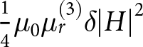$\frac{1}{4}{\mu _0}\mu _r^{\left( 3 \right)}\delta {\left| H \right|^2}$. Since the nonlinear term is much smaller than the linear term at microwave frequencies, <δ> ≈ δ. Therefore, we define the material-dependent parameter δμ_r ⁽³⁾ as the intrinsic nonlinear parameter.

Using Eqs. (9), (11), and (16), the relationship between PIM power and the intrinsic nonlinear parameter is derived.

(19a)\begin{equation}{P_{IM3,{\text{forward}}}} = \frac{{{{\left| {{V_{f,PIM}}} \right|}^2}}}{{2{Z_0}}} = \frac{{9{\pi ^2}}}{{8{Z_0}}}{\left( {I_1^2{I_2}L{f_{PIM}}\frac{{{\mu _0}k_0^3}}{{{W^3}}}} \right)^2}{\left( {\delta \mu _r^{\left( 3 \right)}} \right)^2},\end{equation}

(19b)\begin{align}{P_{IM3,{\text{reverse}}}} &= \frac{{{{\left| {{V_{r,PIM}}} \right|}^2}}}{{2{Z_0}}}\cr &= \frac{{9{\pi ^2}}}{{8{k^2}{Z_0}}}{\left( {I_1^2{I_2}{f_{PIM}}\frac{{{\mu _0}k_0^3}}{{{W^3}}}\left| {\sin \left( {kL} \right)} \right|} \right)^2}{\left( {\delta \mu _r^{\left( 3 \right)}} \right)^2}\!\!\!,\end{align}

where Z ₀ is the characteristic impedance, which is 50 Ω.

LNS-FDTD full-wave method

Since the nonlinear effects of ferromagnetic materials can be described by a nonlinear constitutive equation, their resulting nonlinear responses, such as PIM and harmonics, can be simulated in a full-wave solver by incorporating such a nonlinear constitutive relation. Then, the nonlinear parameters can be extracted by adjusting the nonlinear parameters until the simulated results match the experimental data. Because the nonlinear effect, for example, PIM, is usually weak, the simulation process can adopt the “linearity-nonlinearity separation” method [Reference Zhao, He and Zhang13, Reference Zhao, He and Zhang16]. It should be noted that the thickness of the ferromagnetic coating is typically on the micron scale, which is much smaller than the usual mesh size. Therefore, a special modeling method is required in the full-wave simulation. In the following, a PIM simulation method for ferromagnetic-material-coated microstrip lines is developed, thereby enabling the extraction of third-order nonlinear parameters via full-wave simulation.

Let’s start with the nonlinear constitutive equation for an isotropic ferromagnetic material with third-order magnetic nonlinearity.

(20)\begin{equation}B = {\mu _0}{\mu _r}H + {\mu _0}\mu _r^{\left( 3 \right)}{\left| H \right|^2}H,\end{equation}

where B is the magnetic flux density.

Neglecting the nonlinear term in Eq. (20), its zeroth-order approximation is given by:

(21)\begin{equation}{B_0} = {\mu _0}{\mu _r}{H_0}.\end{equation}

By subtracting Eq. (21) from Eq. (20), we have:

(22)\begin{equation}{B_p} = {\mu _0}{\mu _r}{H_p} + {\mu _0}\mu _r^{\left( 3 \right)}{\left| H \right|^2}H,\end{equation}

where 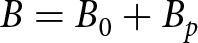$B = {B_0} + {B_p}$, and $H = {H_0} + {H_p}$.

Because the nonlinearity is usually weak for microwave applications, we simplify Eq. (3) to be

(23)\begin{equation}{B_p} = {\mu _0}{\mu _r}{H_p} + M,\end{equation}

where $M = {\mu _0}\mu _r^{\left( 3 \right)}{\left| {{H_0}} \right|^2}{H_0}.$

Let the surface tangential magnetic field be H ₀(t). Under the good-conductor approximation, the field inside the conductor decays approximately exponentially:

(24)\begin{equation}{H_0}\left( {z,t} \right) \approx {H_0}\left( t \right)\exp \left( { - {z \mathord{\left/ {\vphantom {z \delta }} \right. } \delta }} \right).\end{equation}

The equivalent surface magnetization is defined as the depth integral of the volume magnetization:

(25)\begin{align}{M_s}\left( t \right) &= \int_0^\infty {M\left( {z,t} \right)dz} \cr &= \int_0^\infty {{\mu _0}\mu _r^{\left( 3 \right)}{{\left| {{H_0}} \right|}^2}{H_0}dz} \cr &= \frac{1}{3}{\mu _0}\left( {\delta \mu _r^{\left( 3 \right)}} \right){\left| {{H_0}\left( t \right)} \right|^2}{H_0}\left( t \right).\end{align}

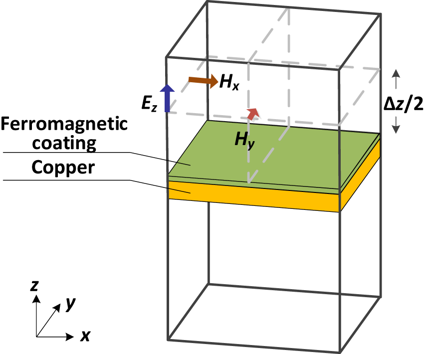
To incorporate this source term into the FDTD update equations, it must be converted into a volume magnetic current density acting on the magnetic-field grid. Physically, this corresponds to “spreading” the surface-concentrated magnetic current over the nearest half-grid thickness (Δz/2), because the tangential magnetic field is defined only on the surface center of the Yee mesh grid as shown in Figure 3.

Figure 3.

The definition positions of the tangential magnetic fields do not coincide with the conductor surface in the Yee grid.

Therefore,

(26)\begin{equation}{M_v}\left( t \right) = \frac{2}{{\Delta z}}{M_s}\left( t \right) \approx \frac{2}{{3\Delta z}}{\mu _0}\left( {\delta \mu _r^{\left( 3 \right)}} \right){\left| {{H_0}\left( t \right)} \right|^2}{H_0}\left( t \right){\delta _{k,{k_{suf}}}}.\end{equation}

where δ_{k, ksurf} is the Kronecker delta, which ensures that the source term exists only at the surface layer.

According to Maxwell’s equations, we have:

(27)\begin{align}\nabla \times {E_p} &= - \frac{{\partial {B_p}}}{{\partial t}} = - \frac{{\partial \left( {{\mu _0}{\mu _r}{H_p} + M} \right)}}{{\partial t}} \cr &= - {\mu _0}{\mu _r}\frac{{\partial {H_p}}}{{\partial t}} - \frac{2}{{3\Delta z}}{\mu _0}\left( {\delta \mu _r^{\left( 3 \right)}} \right)\cr &\quad\times\frac{{\partial {{\left| {{H_0}\left( t \right)} \right|}^2}{H_0}\left( t \right)}}{{\partial t}}{\delta _{k,{k_{suf}}}}.\end{align}

Thus, the equation for the nonlinear part field is obtained, and we use it in the FDTD solver to simulate PIM of the ferromagnetic-material-coated microstrip line. The implementation of the simulation can refer to [Reference Zhao, He and Zhang13, Reference Zhao, He and Zhang16]. Eq. (27) shows that only the intrinsic nonlinear parameter δμ_r ⁽³⁾ is unknown. Therefore, if we compare the experimental data with the simulation results, we can extract this parameter.

Intrinsic nonlinear parameter extraction of Ni coating

PIM experiments

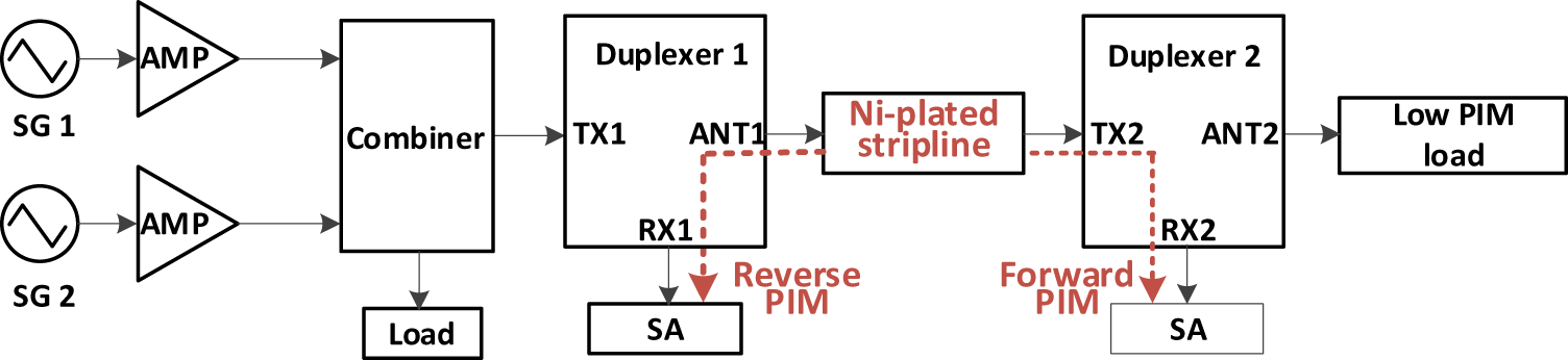
This section validates the nonlinear parameter extraction method by plating a nickel layer on a microstrip line and measuring its PIM effects. The microstrip line is fabricated using a copper-clad laminate with a dielectric constant of 3.5 and a thickness of 1 mm, and a 0.5-oz nickel layer is electroplated onto its upper conductor, as shown in Figure 4(a). The PIM measurement equipment (BXT Technologies) is shown in Figure 4(b). The schematic block diagram of the measurement setup is given in Figure 5. Two carrier signals are set at 728 and 746 MHz, respectively. After amplification, they are combined and fed through Duplexer 1 into the microstrip line under test. The transmitted carriers continue through Duplexer 2 and are absorbed by a low-PIM load. The intermodulation products generated by the nickel-plated microstrip line propagate toward both its input and output ports. The PIM signal traveling toward the input port passes through Duplexer 1 and is sampled by a spectrum analyzer, which is referred to as the reflected PIM. The PIM signal traveling toward the output port passes through Duplexer 2 and is sampled by the spectrum analyzer, which is termed the transmitted PIM. In this experiment, the third-order PIM signal at 710 MHz is measured.

Figure 4.

Photos of (a) the nickel-plated microstrip lines and (b) the PIM test equipment.

Figure 5.

Schematic diagram of the PIM test system.

Figure 5 Long description

On the left, two Signal Generators (SG 1, SG 2) connect via Amplifiers to a Combiner. The combined signal enters Duplexer 1 via the TX port and exits via the ANT port. The signal then passes through the Device Under Test (DUT): a nickel-plated microstrip line. After the DUT, the signal enters Duplexer 2 via its ANT port and terminates at a Low PIM Load. Reverse PIM is measured at the RX port of Duplexer 1 using Spectrum Analyzer 1. Forward PIM is measured at the RX port of Duplexer 2 using Spectrum Analyzer 2.

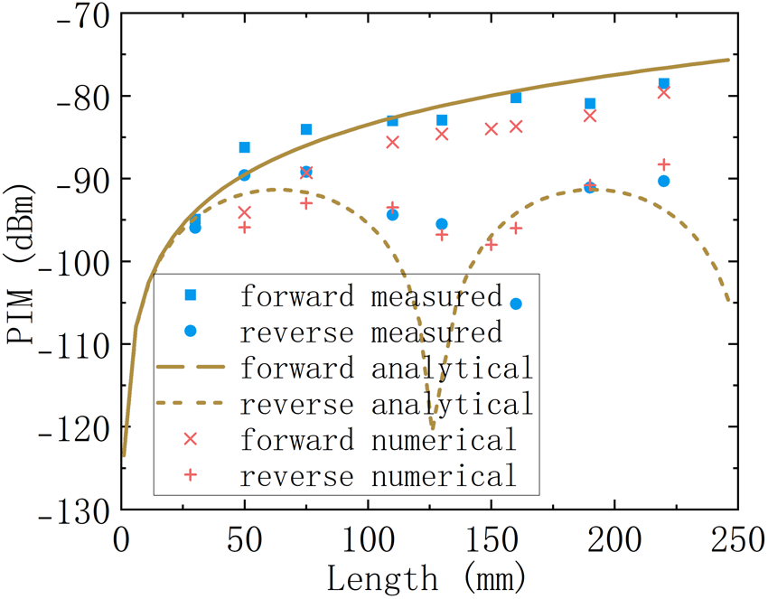
The experimental results are shown in Figure 6. It indicates that as the microstrip line length increases, the forward PIM gradually rises while the reverse PIM exhibits oscillatory behavior, which is consistent with the experimental findings by other researchers [Reference Kozlov, Shitvov and Schuchinsky12].

Figure 6.

PIM results as the function of the length of the microstrip line obtained from the experiments, the coated-microstrip-line-model analytical equations, and the LNS-FDTD full-wave numerical calculation. The experimental data are obtained from Ref. [17].

Figure 6 Long description

This line graph plots Passive Intermodulation (PIM) levels in dBm on the y-axis against the Length of the microstrip line in millimeters on the x-axis (range 0–250 mm). The graph displays six curves representing three different methods: experimental measurements, analytical equations, and LNS-FDTD numerical calculations. Each method includes data for both forward and reverse signal transmission directions. The legend indicates that “forward measured” (blue squares) and “reverse measured” (blue circles) represent the experimental data. The analytical model is shown with yellow dashed lines, and the numerical calculations are represented by red crosses and plus signs. The curves illustrate how PIM levels generally increase with the length of the microstrip line for all tested methods.

Based on the formulas for forward and reverse PIM derived from the coated transmission-line model, Eq. (19), the experimental data are fitted. Here, the input currents I ₁ and I ₂ can be calculated from input power, leaving δμ_r ⁽³⁾ as the only unknown parameter. By performing the fit, the value of δμ_r ⁽³⁾ can be extracted. According to the fitting results shown in Figure 6, it is found that δμ_r ⁽³⁾ = 0.48 × 10⁻¹⁰ m³/A².

For the LNS-FDTD full-wave method, since δμ_r ⁽³⁾ is also the only unknown simulation parameter, an appropriate value of δμ_r ⁽³⁾ is adjusted until the simulation results match the experimental measurements, thereby determining the parameter δμ_r ⁽³⁾ = 1 × 10⁻¹⁰ m³/A². The corresponding simulation results are also shown in Figure 6. It can be seen that the nonlinear parameters obtained by the transmission-line method and the full-wave method are in good agreement, which verifies the feasibility of the proposed extraction method. Taking the ratio of the two to evaluate the deviation between the two methods, the deviation is given by $e = \frac{{1 \times {{10}^{ - 10}}}}{{0.48 \times {{10}^{ - 10}}}} = 6.4{\text{dB}}{\text{.}}$

Limitation of the extraction methods

In the transmission-line method, an equivalent circuit model is employed to derive the analytical expressions for the PIM of the ferromagnetic-material-coated microstrip line. A key assumption that could introduce error is the coupling efficiency ξ ≈ k ₀. This coupling coefficient represents the efficiency with which the nonlinear field generated in the ferromagnetic-material coating couples back into the microstrip line and is subsequently absorbed by the load. In reality, however, because the nonlinear field is primarily generated above the microstrip line, a significant portion is lost due to radiation. Only a fraction of couples back into the line, resulting in an actual coupling efficiency ξ < k ₀. Therefore, this can lead to an underestimation of the extracted nonlinear coefficient.

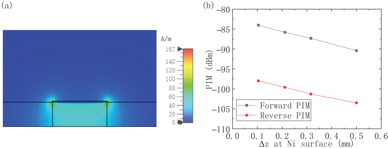
Furthermore, the proportionality coefficient k₀ also needs further discussion. As shown in the magnetic field distribution in Figure 7(a), the current density on the upper and lower surfaces of the upper conductor is not uniform across the conductor width. In the fitting performed in the “PIM experiments” section, the ratio of current densities at the center of the conductor was taken as the value of k ₀, which is obtained to be 0.17. We note that this approach for determining k ₀ also requires further investigation to improve the accuracy of nonlinear parameter extraction.

Figure 7.

(a) The H_x field distribution of the coated microstrip line; and (b) the calculated PIM as a function of the mesh size ∆z at the nearest grid of the nickel surface.

Figure 7 Long description

This figure consists of two parts. Subplot (a) is a 2D heatmap showing the Hx magnetic field distribution (A/m) around a coated microstrip line. A key feature is the visible field intensity difference between the top and bottom surfaces of the upper conductor, attributed to the presence of the dielectric substrate, which alters the field confinement. Subplot (b) illustrates the convergence analysis of the numerical simulation. It plots PIM levels (dBm) against the mesh size (Δz) at the nickel surface. The graph demonstrates that as the mesh size decreases (grid refinement), both the forward and reverse PIM values exhibit a slight increasing trend. This behavior indicates the simulation is converging towards an asymptotic value as the grid size approaches zero.

With respect to the full-wave method, it is necessary to obtain the magnetic field values at the conductor surface. However, since the conductor boundary lies on the Yee grid boundary, the tangential magnetic field on the conductor surface is not directly defined in the FDTD calculation, requiring interpolation. In this work, we use the magnetic field value at the nearest grid point as an approximation, which we identify as the primary source of error in extracting nonlinear parameters via the full-wave method. Evidently, reducing the mesh size brings the nearest-grid magnetic field closer to the actual surface field, thereby improving simulation accuracy. Figure 7(b) presents the computed PIM values under different nearest-grid mesh sizes. It can be observed that as the mesh size decreases, the PIM tends to increase. Hence, it can be inferred that the nonlinear parameter extracted by the full-wave method will be larger than its actual value.

Due to the constraint of the Courant stability condition, reducing the mesh size requires a corresponding decrease in the time step, which significantly increases the simulation time and thus limits the extent to which the mesh can be refined. In the future, the Hybrid Implicit Explicit (HIE)-FDTD algorithm [Reference Chen18] could be considered, as it relaxes the time-step restriction while still allowing a finer mesh in the z-direction.

As described in the above section, the nonlinear parameter extracted by the LNS-FDTD full-wave method is larger than that obtained by the coated transmission-line model, which is consistent with the above analysis.