Question 1.

Do you specify the GUM with contemporaneous relationships or not; that is, y_t on lagged y_t and current and lagged {z_i,t}, or y_t only on lags of y_t and {z_i,t}? Presumably one can consider both alternatives and compare the outcomes. Do you have any experience with this?

Answer 1.

PcGets can indeed do both, and we have tried both extensively. With contemporaneous relationships, there is the possibility of invalid conditioning (endogeneity, or a lack of weak exogeneity), so the program allows for instrumental variable (IV) selection for the relation of interest: PcGets could also be used for the choice of the relevant IVs themselves (see Hendry and Krolzig, 2004b). We have mainly simulated the case of valid conditioning (i.e., least squares), as that is the arena where the effects of selection per se can be studied, as opposed to investigating the gamut of other econometric problems that are likely to remain in any given empirical exercise. We also have Monte Carlo experience with selecting vector autoregressions (VARs), where the second situation holds (only lagged regressors). This is again relevant to selecting IVs in a time-series context. We have not simulated IV estimation yet, partly because of the technical problem of potentially nonexistent moments and partly because we have been progressing so rapidly on the regression case that it seemed sensible to develop that first, then proceed to the finite-sample properties of selecting in an IV context.

Question 2.

You sometimes do simulations to investigate the performance of the program. What happens if the DGP is not included in the GUM?

Answer 2.

We have done a large number of simulation experiments, first to calibrate the program, then to investigate its operating characteristics and overall performance. In all of these, however, the DGP is nested in the GUM (denoted DGP ⊆ GUM) as we also wished to test our theory of model selection. Much of the model selection literature is pessimistic about search and attributes quite high costs to searching for a model in a morass of irrelevance, unless the sample is large relative to the number of candidate variables. The classic study is Lovell (1983).

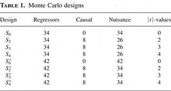
However, that is far from our experience with PcGets. Table 1 records the form of one set of simulation experiments (a subset from Hendry and Krolzig, 2004a). The sample size is T = 150, all variables are white noise, and the number of irrelevant variables N is either 26 (experiments S₂–S₄) or 34 (experiments S₂*–S₄*) in matching pairs. There are either none or eight relevant variables, where all t-values are equal within experiments (to allow us to compute outcomes in the more likely situation when there is a mixture). The noncentralities of the eight relevant variables' t-tests are successively all 2, then all 3, then all 4, respectively (shown by the subscript of the experiment), so S₀ has a null DGP.

Monte Carlo designs

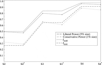
The outcomes are recorded in Figure 1 in Section 4 (the two strategies called Liberal and Conservative are defined in the answer to question 6 but are approximately 5% and 1% per test, respectively). They will be discussed in detail shortly, but the graph suggests that search costs per se are remarkably low as there is little difference in outcomes between matching S_i and S_i*.

Our heuristic explanation for the success of PcGets regression searches where all variables are mutually orthogonal is as follows: rank the squared t-tests on each variable in the GUM and retain all and only those that exceed the preset significance level—thus, the final model is actually selected by a single decision. Consequently, “repeated testing” is not involved: the problem of chance significance is really sampling fluctuations, not search. However, the probabilities of observing any given squared t-values in excess of the desired critical value are altered by the numbers of relevant and irrelevant variables. Some of the apparent repeated testing in modeling algorithms is due to collinearity making the initial t-test ranking useless, thereby enforcing a search for what the “real” t-values are. Notice, therefore, that in all our experiments, misspecification testing has simply been a cost, with no possible benefits, since no GUMs were misspecified.

When the DGP is not nested in the GUM, there nevertheless exists a “local DGP” (denoted LDGP), namely, the derived distribution in the space of the variables under consideration, obtained by marginalization, conditioning, and so on: this follows from the theory of reduction (see, e.g., Hendry 1995; Bontemps and Mizon, 2003). Then two possibilities arise. In the first, an empirically congruent representation can be achieved, in which case we would expect PcGets to be judged by how well it located that LDGP. For example, the DGP may involve an AR(1) variable that is not observed, generating an autoregressive moving average (ARMA) error, approximated in turn by using longer lags on the variables that are observed, such that the final residuals do not depart significantly from a martingale difference sequence. In the second possibility, the LDGP cannot be well approximated by the specified GUM, so congruence is violated. Now misspecification testing at least reveals such a problem exists. Two routes are then open:

Question 3.

Are there any advantages or disadvantages in using a small or large GUM: if the DGP is in the GUM, is it less likely to be found when starting with a large GUM?

Answer 3.

This trade-off is important and is discussed in Hendry and Krolzig (2001). If the DGP ⊆ GUM, it is less likely to be found when starting with a larger GUM, in that there is a higher probability of retaining one or more of the additional irrelevant variables by chance, and if the setting is not orthogonal, also a higher probability of omitting relevant variables. Thus, conditional on DGP ⊆ GUM, the smallest possible GUM is best: prior simplification pays, which allows an important role for theoretical reasoning about what is excluded as well as what variables should be included. However, the obvious danger is that a priori simplification could lead to relevant variables being omitted, violating DGP ⊆ GUM, in which case one will never locate the DGP. Thus, it is essential to devote considerable prior thought to specifying the GUM, which is obviously crucial to the success of the search.

Question 4.

Is it more or less likely that the DGP will be embedded in the final model if one starts with a small GUM rather than a larger one, assuming that the true DGP is in the GUM?

Answer 4.

In an orthogonal specification, additional irrelevant variables should not greatly affect whether the DGP is embedded in the final model. As we have just noted, the costs of additional orthogonal variables are small: matching pairs of S_i and S_i* show only a small decrease in the probabilities of retaining relevant variables. However, if there is considerable intercorrelation between all variables (relevant and irrelevant), then a larger GUM is likely to reduce the probability of retaining relevant variables, and hence the DGP may not be embedded in the finally selected model.

Question 5.

What happens if z_1,t and z_2,t are highly collinear, such as alternative definitions of some economic variable, in particular when (a) one of the z_i,t belongs in the DGP; or (b) when neither does?

Answer 5.

Collinearity is dependent on the parameterization adopted rather than being intrinsic to a model: for example, (1) is invariant under linear transformations. Moreover, there are three possibilities: (i) neither variable matters; (ii) only one of the variables matters; (iii) both matter. The first is easiest: one variable will be immediately eliminated, and the second should then follow, subject to the usual probability of adventitious significance. Alternative definitions of an economic variable, however, are an example of (ii), where only one matters. I assume the one matters importantly (i.e., with a large t-value), and conditional on the correct choice, the other is irrelevant. Then the behavior of PcGets depends on its settings. If only multipath searches are used, each of z_1,t and z_2,t will constitute the start of an elimination path, with the other provisionally retained, and therefore a terminal model with each will almost surely be found. These are then subject to an encompassing comparison, and if that is indecisive, a model selection criterion, such as that due to Schwarz (1978) (denoted SC), is used. The collinearity between z_1,t and z_2,t is not the real problem; rather what matters is whether or not the “true” determinant empirically has a higher correlation with y_t in the observed sample. However, if presearch tests were used, the one of the two with the smaller marginal contribution in the GUM would almost certainly be eliminated, leaving the other to win the day.

This difference in search strategy becomes crucial when perfect collinearity holds: for example, an investigator may be unsure which of the combinations of z_t, z_t−1, and Δz_t determines y_t. It may surprise econometricians, but all three variables can be entered, and if only path searches are used, the correct combination can be selected. We conducted four small one-off experiments where, in turn, y_t depended on (a) z_t and z_t−1; (b) z_t and Δz_t; (c) z_t−1 and Δz_t; and (d) Δz_t; but in each case all of z_t, z_t−1, and Δz_t were entered as regressors in the GUM. PcGets gave the correct answers in (b), (c), and (d) but rather amusingly in (a) selected the equivalent, but more orthogonal, representation, z_t−1 and Δz_t. This is an example of how our new tool yields new insights: one might have suspected that perfect collinearity was insoluble, but having tried the preceding idea, we have found it can work. However, presearch tests would arbitrarily eliminate whatever variable the inversion routine happened to treat as redundant, which may even depend on the order in which they were entered in the regression (see Hendry and Krolzig, 2004b).

Finally, concerning (iii), there are two aspects, one related to the intercorrelations, which can be removed by an orthogonal transformation, and one related to the net information content in (say) z_2,t given z_1,t, which determines the net noncentrality of the least significant component after orthogonalizing. As Hendry and Krolzig (2001) note, two random walks with drift can be intercorrelated 0.999, yet there is no problem in finding the correct specification, whereas the same correlation between two regressors from a standardized bivariate normal will usually ensure failure to retain both variables when both matter. In that latter case, the net contribution of the marginal component is negligible. The Monte Carlo experiments in Hendry and Krolzig (2004a) show that size and power are adversely affected by this effect, even in the correctly orthogonalized representation.

Question 6.

If, in the reduction process, you use a criterion like |t| ≥ 2 for a parameter estimate, can the modeler chose a more parsimonious criterion, such as |t| ≥ 2.5, say? Are there any examples of what is found?

Answer 6.

The user can set any selection criterion level, from tight to loose. PcGets has two preprogrammed settings, and when T is about 100, one is based around |t| ≥ 2 (i.e., approximately 5%), called the Liberal strategy, and the other around |t| ≥ 2.625 (i.e., roughly 1%), called the Conservative. Both strategies use critical values that depend on T, and for large samples on N, the former converging to the critical values corresponding to the criterion proposed by Hannan and Quinn (1979), denoted HQ, and the latter to SC. Both Liberal and Conservative are much more stringent in small samples than HQ and SC, respectively. We have extensive experience with both strategies, and their relative costs and benefits, which depend on the nature of the problem. If there are many potentially irrelevant variables and few relevant but with high significance, the Conservative strategy outperforms (e.g., the Hoover and Perez, 1999, rerun of the Lovell, 1983, “data mining” experiments); whereas for few irrelevant and many relevant, perhaps with |t|-values around 2–3, Liberal is far better. Indeed, in the latter experiments, the Liberal strategy commencing from a highly overparameterized GUM outperforms the Conservative commencing from the DGP, emphasizing the importance of the choice of strategy.

Figure 1 shows the comparative probabilities of retaining relevant variables by the Liberal (solid line with points) and Conservative (dashed line with points) strategies for an equation like (1) from the experiments in Table 1. When N is either 26 (experiments S₂–S₄) or 34 (experiments S₂*–S₄*), the Liberal strategy will on average retain 1.3 or 1.7 irrelevant variables per trial as adventitiously significant at 5%, whereas the Conservative will keep only 0.26 or 0.34—that is, roughly one variable significant by chance every three equation selections. Conversely, the power loss of Conservative over Liberal is about 0.15 at t = 2, falling to under 0.1 at t = 4: that is a large cost to ensure that almost no irrelevant variables are retained.

Probabilities of retaining relevant variables.

However, the expected powers for testing in scalar t-distributions with those noncentralities and 100 degrees of freedom are easily calculated at 5% and 1% and are shown by the dotted and long dashed lines, respectively. There are several implications. First, both strategies are close to their theoretical upper bounds (the slight crossovers are due to the null rejection frequencies not being precisely 5% or 1%, respectively). Second, the apparent power loss of the 1% stringent rule relative to the 5% is to be expected, even if neither search nor selection was involved: it is primarily a cost of inference, not of search. Third, the “power gap” between them narrows as the noncentrality rises, so the costs of the Conservative strategy are lower at higher powers. Finally, there is almost no “power” difference between S_i and S_i*, a comparison I noted in answering your question 2. Intermediate significance levels, such as 2.5% (|t| ≥ 2.275), can be reasonably inferred from these results: for instance, 0.65 and 0.85 irrelevant variables retained on average, with powers of 0.39, 0.76, and 0.96 for t = 2, 3, 4, respectively.

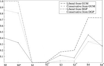
Some researchers try to interpret the overall selection procedure in terms of size and power, namely, how often will the selected model retain any irrelevant variables, and how often will it keep all the relevant? For these experiments, such results might seem depressing: the overall “sizes” are 0.74 and 0.83 at 5% and 0.23 and 0.29 at 1%; and the overall powers 0.004, 0.25, and 0.82 at 5% and essentially zero, 0.03 and 0.49 at 1%. Together these translate into low probabilities of locating the DGP. However, even if one commenced from (2) as the initially postulated model, rather than (1), but still had to conduct the usual statistical tests of misspecification and coefficient significance, the DGP would almost never be retained, particularly using the Conservative strategy. Figure 2 (another subset from Hendry and Krolzig, 2004a) illustrates. Here S₀ and S₀* denote experiments with no relevant variables, so the DGP is bound to be kept if it is the starting hypothesis. The Conservative strategy nonetheless does fairly well in that setting, locating the null between 85% and 80% of the time, notably higher than the frequencies of 77% and 71% predicted by the preceding “size” calculations. This difference reflects that PcGets uses block F-tests in addition to t-tests in its decisions: when the null is true, F-tests at even loose significance levels will sometimes lead to all variables being excluded before search, improving its performance in that null setting at little cost in others but adding to the difficulty of deriving its properties analytically.

Probabilities of locating the DGP.

Notice that S₂ and S₂* are never found, even when commencing from the DGP. Thus, the basic problem is one of lack of significance, a cost of inference, not one induced by searching per se. Conducting only absolute comparisons—like the probability of getting the correct answer—while failing to standardize by the relative comparison of knowing the DGP delivers a misleading picture of how well search performs. Experiments S₃ and S₃* are even more enlightening: the Liberal strategy commencing from the GUM dominates the Conservative strategy commencing from the DGP. Moreover, with even 26 irrelevant variables, there is little difference between commencing from the DGP or GUM, although that gap grows for 34 irrelevant. I doubt the empirical relevance of such large numbers of irrelevant variables in macroeconometrics, although I can see micro and finance situations where it is all too likely (see, e.g., Sullivan, Timmermann, and White, 2001). Finally, the outcomes in S₄ and S₄* are now predictable: knowing the DGP and using Liberal really pays, since almost all relevant variables are retained, and no irrelevant; and the Liberal strategy from the GUM still outperforms the Conservative strategy commencing from the DGP for 26 irrelevant but not for 34. The outcomes for |t| ≥ 5 follow logically: all probabilities will be higher, but the Conservative strategy will now outperform Liberal, confirming a

-shaped relation for choice of strategy as a function of the average noncentrality, with a monotonic benefit from stringency as the number of irrelevant candidate variables increases.

Question 7.

Is it possible to relax some of the basic requirements of the procedure, such as that models satisfy a Chow test or that residuals are normally distributed? Do you have experience whether such relaxations produce a very different final model?

Answer 7.

The actual operation of PcGets is more sophisticated than it may appear at first sight, in that it is programmed to make decisions about test rejections as follows. Say normality is rejected at the initially set significance level (e.g., 1%). First, a much tighter level is checked (say, 0.1%, preprogrammed as a function of the initial level), and if that also rejects, then the test is “suspended” for the analysis. The user is alerted, and it is assumed the user will either change the GUM to alleviate the difficulty or did not deem normality to be important for congruence. If the tighter level accepts, then that is used for the associated test during simplification—but now regarded as a diagnostic of the validity of reductions—such that path searches will be terminated if that tighter level is violated. We adopted such an approach because overparameterized dynamic models can induce (e.g.) significant negative residual autocorrelation. We do not have much simulation experience on the impacts of dropping tests when there is a genuine problem, since all the simulations have DGP ⊆ GUM. However, my practical experience is that such rejections at the 1% level or smaller almost always signify misspecifications of the GUM for the LDGP when empirical data are analyzed, especially if it is parameter constancy that is rejected. Conversely, for Monte Carlo response surfaces—where PcGets can be invaluable given very large numbers of potential regressors—several tests of functional form may reject without implying a poor descriptive representation.

Question 8.

A theory sometimes puts constraints on groups of parameters, either within a single equation or across equations. Can such constraints be accommodated in the program, or should you just run it and test if the constraints hold?

Answer 8.

Some classes of constraints can be imposed already, namely, those that deliver a specific numerical combination of variables, such that the remainder ought then to be insignificant. At the request of several users, Hans-Martin and I have recently been addressing the issue of sign restrictions. At present, sign restrictions are not handled: users must simply delete the offending variable(s) from the GUM and restart if violations occur. We instead propose that first the signs be tested in the GUM. If they are rejected, then there is no feasible congruent simplified model satisfying the constraints, so the user needs to rethink and respecify the GUM itself. However, if the restrictions are accepted at the preassigned significance level, then they are imposed during simplification as constraints precisely like the diagnostic tests—a violation terminates a search path as inadmissible. Then the final model is guaranteed to satisfy the constraints and be a valid, congruent reduction that will parsimoniously encompass the GUM. Even so, one should always run the program and check if the constraints hold anyway: if so, the best model has been found. If not, then it is worth recording the costs of the constraints even if an acceptable model satisfying them has been located. The cross-equation variety will follow once a systems-based algorithm has been developed (see Section 7).

When there are competing theory models of a given variable, PcGets could be used to select the “best representative” of each theory, given their information sets and entailed GUMs. That would allow encompassing tests to be used to determine their relative performance, albeit without precluding that a union could dominate either alone.

Question 9.

There are some occasions when a model's purpose requires that certain variables remain in its specification, such as policy variables in a model designed to study policy scenarios. Can the program specify that designated variables not be dropped in the reduction process?

Answer 9.

Yes, PcGets already provides such a facility: variables can be denoted as “fixed” so must enter all specifications, including the final selected model. In Hendry and Krolzig (2001), we recommend that a user run the program both with and without “fixed variables” and, if the models differ, conduct an encompassing test between them. Naturally, the “null” is the restricted formulation, as that is deemed theoretically preferable, so a stringent critical value is allowable, but equally, there must exist some level of significance at which the theory—and entailed policy—should be questioned. Further, the forcibly retained variables need not be significant—and may even have signs that clash with the theory, perhaps remedied by answer 8.

However, our latest research has resolved another important aspect of model selection for policy analyses, where unbiased and small variance estimates of policy derivatives are paramount. Selecting by discrete criteria, such as

where α is the significance level of the test, and eliminating otherwise, leads to what is called “pretest” bias, since the estimated coefficient

is a weighted average of the value when retained and zero when eliminated. That result refers to the unconditional distribution of the estimator, which does not seem relevant given the decision rule. The relevant distribution is the conditional, namely,

, say, as that is the estimate in the selected model, and now

must be biased away from zero (“small” estimates are not retained). That bias can be corrected in substantial measure, without much increase in root mean square errors (RMSEs) when variables are relevant and with a substantial reduction in RMSEs when variables are irrelevant. That may sound too much like a free lunch, but it follows from knowing that unrestrictedly,

is approximately normally distributed, so

is a truncated normal, where the truncation rule

is known. Thus, like the results in (say) Heckman (1976), the selection bias can be approximately corrected. Preliminary results are presented in Hendry and Krolzig (2004c).

Question 10.

Do all variables have to be I(0), or can one have a mixture of I(0) and I(1)?

Answer 10.

Variables can be a mix of I(0) and I(1) in principle, but there are important caveats. Unless PcGets “knows” what their integrability properties are, it cannot make correct inferences, as all critical values are based on conventional asymptotics at present (this is not an issue of principle, merely program complexity). Providing the GUM formulation ensures that all specification hypotheses to be tested correspond to I(0) inferences as in Sims, Stock, and Watson (1990), then no invalid inferences will be conducted: for example, in a scalar process y_t, if it is I(1), a test of the significance of y_t−1 will use incorrect critical values but must inevitably reach the correct decision that y_t−1 matters. The F-test of the null of no relation would use the wrong reference distribution but would also correctly reject, given that the alternative is indeed true. Misspecification tests on the GUM, and any reduced models thereof, will be fine as well: see, for example, Wooldridge (1999). However, a user could formulate a specification that violates this setting, namely, with Δy_t as the dependent variable when y_t−1 is a regressor, in which case conventional critical values are incorrect (see, e.g., Dickey and Fuller, 1981). We tend to advise nonexperts to enter all variables in levels (after appropriate functional form transformations) and allow PcGets to make the decisions about I(0) transforms (cointegration and differencing), as well as relevance.

Question 11.

If y_t is I(0) and a pair of z_i,t are I(1) and cointegrated, are they both likely to occur in the final model?

Answer 11.

If y_t is I(0) when a pair of z_i,t are I(1) and cointegrated, then either both or neither are virtually certain to occur in the final model, the former if their cointegrated combination matters, the latter if it does not. That claim is based on theory and experience and some pilot Monte Carlo evidence: it would be easy to conduct a range of relevant simulations; t-tests of the null that each z_i,t was irrelevant would again use the wrong reference distribution under the null, and so be slightly oversized, but correctly reject under the alternative.

Question 12.

Can you build an error-correction model with PcGets with an extension of adding further explanatory I(0) variables?

Answer 12.

PcGets “nonexpert” mode requests only the list of basic regressors (i.e., before lags but after functional form transformations), chooses the lag length, checks for cointegration, transforms to I(0), and then selects the relevant subset of regressors. The final model, therefore, has an equilibrium-correction component if cointegration occurs between y and the zs, as well as I(0) differenced regressors. Any levels variable, even an I(0) one, would be “attributed” to the cointegration combination, which makes sense since all I(0) variables must be cointegrated, but this would underestimate the uncertainty in the final model's coefficients. Again, we have not yet conducted the relevant simulations of its performance but plan to do so. Reestimating a variety of published specifications suggests it does remarkably well against experts.

Question 13.

Are there any constraints on the dependent variable y_t? If I can model y_t, can I also model |y_t| or y_t²; that is, some measure of risk? Here the assumption of normality would not be appropriate.

Answer 13.

We have not tried modeling nonlinear functions of the dependent variable such as |y_t| or y_t². The principles are unaffected, although as you note, the considerations discussed in answering question 6 seem likely to intrude. If congruence required (say) an error distributed as a chi-square, it would be good to test against that, and no methodological issue precludes doing so, although in practice we have not programmed such cases (PcGive does allow QQ plots against, say, χ², so we could allow for similar forms of comparison in later releases; see Hendry and Doornik, 2001).

Question 14.

If I have a regression of the form

can I estimate λ by trying a number of possible values, say, λ = 0, or 0.2, or 0.4, or 0.8, or 1, and then compare models? Or, should I put all z_1,t^λs with these λ values into the GUM?

Answer 14.

We have recently started on the theory for selecting nonlinear models but have not tried any specific approaches. However, I suspect the best approach is optimizing over λ subject to ensuring that β₁ ≠ 0 (for identifiability). A general nonlinear GUM might be a more useful initial specification, such that specific forms like z_1,t^λ are reductions to be tested for validity.

Question 15.

As the program just uses y_t and a vector of z_i,t variables, it can presumably be used to estimate a model of the form

where the functions g(·), h_i(·) are given. A variety of alternative h_i(·) functions could be used in the GUM. Do you think this is plausible? Have you any experience with this?

Answer 15.

I assume you intend to include all the “variety of alternative h_i(·) functions” simultaneously in the GUM. Then the answer is rather like that to question 14. However, on a different interpretation, this also relates to question 10: at present users are required to prespecify appropriate functional form transformations, which is often difficult. Consequently, automating that choice would be beneficial. There are at least six important problems needing to be resolved. First, there is the specification problem: what class of functions g(·) and h_i(·) are relevant? Presumably these are specified by the user on the basis of theoretical analyses. Second, can one determine a general functional form approximation for a GUM within which reductions to anticipated g(·) and h_i(·) can be evaluated? Often polynomial approximations are used, but other systems of approximating functions merit consideration. Third, there is a computational problem: how to efficiently investigate that class? Polynomials can be orthogonalized, so that would seem a useful basis, but are not obviously the best choice. Next, a general functional form may involve more potential variables than observations (i.e., N > T). Surprisingly, this need not be a problem for PcGets providing n << T (see, e.g., Hendry and Krolzig, 2004b), confirming that the new tool can also solve previously intractable problems. Fourth, there is the statistical problem of controlling rejection frequencies if the class of functions or approximations considered is very large. A rule for setting critical values, once k + m < T, could be based on being at least as stringent as SC, but converging to SC as T and N diverge to ensure consistent selection. Finally, there is an identification problem when some parameters vanish under the null, affecting the reference distributions. This would need to be circumvented by ensuring that postulated g(·) and h_i(·) functions first effected a significant reduction. There are many interesting research avenues to be explored here, but again the tool itself highlights new perspectives on how to proceed. We are comparing the performance of PcGets with the relevant transformation of the inputs network approach (RETINA) of Perez-Amaral, Gallo, and White (2003, this issue), which is explicitly oriented to selecting nonlinear representations. Their findings suggest both approaches have advantages in some settings, so aspects of their work will undoubtedly enhance how a generic automatic approach performs.

Question 16.

I understand that PcGets can be used to estimate a vector autoregression. What cost function is used for this model? For the original VAR, it may be possible to use least squares separately for each equation because of the “seemingly unrelated” property. However, after some reduction, this would no longer hold.

Answer 16.

Indeed: after some reductions, least squares separately for each equation would not be optimal but would remain feasible, if inefficient. This is the present implementation, awaiting programming of a system likelihood-based approach. This will include vector tests across variables, such as the longest lag on every equation, and so on, in a full VAR implementation. The efficiency issue is explicitly addressed in Krolzig (2003). When the reduced-form VAR has a diagonal covariance matrix, then all possible reductions of the system can be efficiently estimated by ordinary least squares (OLS), and model-selection procedures can operate equation-by-equation without any loss in efficiency. For a structural VAR (SVAR), with a recursive specification as in Wold (1949), a similar result holds for OLS being efficient. In Krolzig's Monte Carlo experiments, the PcGets selection procedure recovers the DGP specification from a large unrestricted SVAR with controlled size and with high power relative to the DGP estimates.

Question 17.

People will want to build multiple equation models but may not want to be limited to a VAR format. Could they just build a model using the program for each individual dependent variable? Do you think that the “specification gain” will beat any “estimation loss” from such an approach?

Answer 17.

Yes, one could model each equation separately and for computational reasons will have to do that (or small blocks of closely related variables) for some time to come. I doubt if the “estimation loss” is serious relative to the “specification gain” if GUMs are well thought out. It used to take literally months to explore data and develop dynamic models thereof, and a large part of that burden has been removed for linear specifications, with many other model classes to follow. Simultaneous cointegrated systems are in principle feasible: the system (“reduced form”) is identified, and simultaneity is merely another reduction that replaces a linear combination of many unmodeled variables by a few combinations of endogenous variables, so identification is easy to maintain in that framework: Krolzig (2003) makes several proposals, since extended in Hendry and Krolzig (2004b). Cointegration selection algorithms already work—see Omtzig (2002). A general likelihood-based selection algorithm of this form would, of course, also efficiently solve the VAR selection problem you raised in the previous question.

Question 18.

Forecasting density functions is an interesting current topic but not an easy one in practice. One method could be to model cos(qy_t) and sin(qy_t) for various values of q. From these one can get an estimate of the conditional characteristic function, from which the conditional density function can be derived. Can you see any obvious problems with the approach? Perhaps the z_i,t variables could be transformed to be in the (−1,1) region. Extending the idea of modeling transformations of the dependent variable, could one consider exp(qy_t) and directly obtain an approximation to the moment generating function?

Answer 18.

Forecasting remains on the research agenda for the moment. We have seen the main task of our research as establishing the properties of Gets methods of selecting models relative to the DGP. Once one has discovered that such an approach to model selection is not distortionary, the use of the resulting models for forecasting in stationary processes merits analysis. Some preliminary results are provided by Brüggemann, Krolzig, and Lütkepohl (2002), who find that PcGets does well relative to information criteria and usually outperforms using the estimated DGP: the costs of estimating some parameters exceed the benefits from including the corresponding variables.

As yet, PcGets does not have a decision rule explicitly designed for selecting forecasting models. This is because my research with Mike Clements (see, e.g., Clements and Hendry, 1999) has found that nonstationarities are a dominant factor in forecasting performance, particularly unanticipated location shifts. Consequently, adaptability and robustness to such shifts are essential attributes of any forecasting device that hopes to succeed operationally. Other approaches to automatic model selection focus much more on forecasting performance. For example, the original final prediction error (FPE) criterion of Akaike (1969) was explicitly designed for that purpose, albeit for constant-parameter processes. Peter Phillips has pioneered an automated approach that reselects the model specification and reestimates as new information accrues, to ensure adaptability (see, e.g., Phillips, 1994, 1995, 1996, 2003). There are important aspects of his approach that should enhance any automatic selection approach for forecasting.

Question 19.

For conditional density models, one approach is to model quantiles, but this requires the use of nonsymmetric cost functions. Is there any possibility that at some time a wider class of cost functions than just least squares can be used?

Answer 19.

Almost certainly: likelihood is really the basis of PcGets, and that need not coincide with least squares. Selecting in a quantile regression is surely feasible, albeit unresearched.

Question 20.

How do you see new tools like PcGets progressing over the next few years?

Answer 20.

The whole area is bubbling with exciting developments and new ideas: see many of the papers in the special issue on model selection edited by Haldrup, van Dijk, and Hendry (2003) and this volume celebrating the 20th anniversary of Econometric Theory. Any problem that can be tackled by a human investigator is susceptible to programming to ease the burden. Exploring many paths, or many values of auxiliary parameters, or recursively reselecting and reestimating, or investigating many functional forms, and so on, are all problems at which computers have a huge comparative advantage over humans. Thus, I see almost unbounded applications for such methods to relieve the more tedious aspects of modeling, reducing its labor intensity and freeing time for more productive activities.

There is also a major public relations task to be confronted. Some editors and referees have reacted adversely to such work, claiming it “de-skills” econometricians or “loses control” of the creative aspects of modeling. These represent a serious misunderstanding of where the value-added of economists and econometricians arises in empirical modeling. When computers first replaced hand calculations for computing regressions, I remember complaints that “no one will really understand the process”; yet econometrics could not have progressed without computers. Similarly, with automatic selection. I believe model selection will remain essential in an evolving process like an economy to try to exclude the nonconstancies and thereby reduce the potential for forecast failure.

A second class of reactions has been disbelief that “data mining” might actually be a productive activity even when conducted sensibly. The evidence to date is really positive for several approaches, including Gets, and, although in a linear regression context, does establish that search and selection are not pernicious when properly conducted. Compared to the operational characteristics of the approaches investigated by Lovell (1983), great progress has been made in a short time. Symbioses with developments in both computer learning and expert systems must follow soon.

Even though explicit derivations of the sampling distributions of the outcomes from automatic procedures are very difficult, impressive progress has occurred there too, especially in the work of Leeb and Pötscher (2003a, 2003b). Although in their contribution to this volume, those authors are skeptical (see Leeb and Pötscher, this issue), the case they are focusing on is intrinsically problematic, namely, selection to “improve” inference about a specific parameter of interest for one of a set of correlated regressors, when estimation of the constant parameters of the DGP would be inconsistent. In the Monte Carlo simulations in Hendry and Krolzig (2004a), PcGets produces bimodal distributions for the selected irrelevant variables, and that would also occur for “nearly irrelevant” variables (i.e., those with small noncentralities of their t-tests, such as less than unity in absolute value). Such variables would rarely be selected: even |t| = 2 is only found 50% of the time. As noted previously, developing orthogonal representations of models is an integral step in our approach, aimed at locating congruent invariant and parsimonious empirical models, in contrast to (say) “focused inference” (as in Claeskens and Hjort, 2003).

Overall, I anticipate many additional practical developments, as well as further insightful theoretical analyses of finite-sample behavior.