1. Introduction
Asia, the world’s most populous region, is home to approximately 9.5–10.6 million stroke patients annually [Reference Tan, Pandian, Liu, Toyoda, Leung, Uchiyama, Kuroda, Suwanwela, Aaron, Chang and Venketasubramanian1]. Stroke, as a non-communicable disease, and particularly in China, has established itself as one of the leading causes of death and disability among older adults [Reference Tu and o. C. S. S. Report2]. Compared with traditional physical, occupational, and language therapy, robot-assisted rehabilitation technology offers three primary advantages in stroke rehabilitation. First, precise motion control capability: The robot achieves precise motion positioning through an optical encoder and closed-loop control, reducing subjective errors in traditional manipulation [Reference Banyai and Brişan3, Reference Han4]. Second, a standardized training system: The technology features built-in switchable training modes (e.g., virtual scene interaction, resistance training). Real-time calibration of joint trajectories via sensors, combined with closed-loop algorithms, ensures significantly higher standardization of training actions than traditional methods [Reference Hong, Li, Bao, Liu and Jin5, Reference Tam, Tang, Kamsani, Yap, Coffey-Aladdin, Goh, Tan, Lui, Lee, Suresh and Chew6]. Third, a quantitative evaluation system: Rehabilitation robots can collect core data such as joint activity and gait spatio-temporal parameters (e.g., step length, step frequency) through a sensor network. Based on an AI algorithm, they generate real-time dynamic rehabilitation reports with motor function trends, enhancing the objectivity of therapeutic effect evaluation by 50%–60% compared to traditional manual assessments [Reference Park, Lee and Lee7]. According to prior research, various lower limb rehabilitation robots (e.g., Lokomat, HAL, Ekso) have been evaluated in clinical trials at multiple global research centers [Reference Zhang, Yue and Wang8]. Numerous RCTs have demonstrated that robot-assisted rehabilitation outperforms traditional therapy in improving gait independence and long-term outcomes [Reference Rodriguez-Fernandez, Lobo-Prat and Font-Llagunes9, Reference Bettella, Tortora, Menegatti, Petrone and Felice10]. More importantly, in the field of stroke rehabilitation, robot-assisted gait rehabilitation (RAGT) has been recommended as an essential adjuvant therapy by multiple international clinical guidelines (e.g., American Heart Association, Canadian Stroke Guidelines) and consequently has gradually emerged as a common clinical intervention [Reference CalabrÒ, Sorrentino, Cassio, Mazzoli, Andrenelli, Bizzarini, Campanini, Carmignano, Cerulli, Chisari, Colombo, Dalise, FundarÒ, Gazzotti, Mazzoleni, Mazzucchelli, Melegari, Merlo, Stampacchia, Boldrini, Mazzoleni, Posteraro, Benanti, Castelli, Draicchio, Falabella, Galeri, Gimigliano, Grigioni, Mazzon, Molteni, Morone, Petrarca, Picelli, Senatore, Turchetti and Bonaiuti11]. However, varying brain injuries among patients (including lesion location, size, and concomitant neurological deficits) drive clinical heterogeneity. Specifically, prefrontal and parietal lobe damage may impair cognitive functions, while primary motor cortex (M1) lesions disrupt limb motor abilities [Reference Li, Fang, Li and Zhang12]. These anatomical and functional heterogeneities directly determine residual limb motor capacity, influencing neural plasticity and training adaptability. Thus, rehabilitation strategies (including exoskeleton assistance strength, step frequency parameters, and task-oriented training protocols) require dynamic adjustment based on individual injury profiles [Reference Zich, Ward, Forss, Bestmann, Quinn, Karhunen and Laaksonen13].
Diverse lower-limb rehabilitation robots have been developed to meet the varied needs of rehabilitation training for lower-limb movement disorders [Reference Li, Zhou, Dong, Rong and Jiao14]. Motion Maker, a representative lower-limb rehabilitation robot, was developed by the Swiss Federal Institute of Technology [Reference Bouri, Abdi, Bleuler, Reynard and Deriaz15]. The robot has bilateral mechanical exoskeleton legs, which can perform lower-limb rehabilitation training in horizontal lying, inclined lying, and sitting postures. The Lokomat lower-limb rehabilitation robot developed by Hocoma (Switzerland) [Reference Jezernik, Colombo, Keller, Frueh and Morari16] has a global installation base of approximately 1,200 units. However, its widespread clinical adoption has been hindered by its bulky mechanical design, high cost, and restriction to standing gait training. The multi-joint lower-limb rehabilitation robot developed by Yanshan University [Reference Feng, Wang, Lu, Vladareanuv, Li and Zhao17, Reference Wang, Wang, Hu, Tian, Lin, Yan, Niu and Sun18] – capable of enabling both active and passive lower limb training in sitting and recumbent postures – has successfully entered the rehabilitation departments of multiple hospitals [Reference Lu19].
Overall, there have been substantial advancements in lower-limb rehabilitation robots. However, the industrialization process remains protracted. Although these commercial products have certain technological advancements, they have revealed practical limitations such as insufficient adaptability to different patient states and poor flexibility in human–computer interaction in clinical applications [Reference Kapsalyamov, Hussain, Goecke, Brown and Jamwal20]. These limitations reflect the technical bottlenecks of robot systems in adaptability and flexibility of human–machine cooperative control [Reference Centeno-Barreda, Salazar-Cruz, López-Gutiérrez, Rosales-Luengas and Lozano21]. The key to enhancing the adaptability of rehabilitation robot systems to patients lies in adequately accounting for human–machine contact interaction [Reference Li, Wei, Zhang and Liu22] and establishing an accurate human–machine dynamics model [Reference Sun, Hu, Gao, Gao, Ma and Wang23, Reference Zhang, Zhang and Elsabbagh24]. Solving the problem of human–machine collaborative control compliance – and thereby enhancing rehabilitation comfort [Reference Yang, Yin, Qi, Li, Zhou, Liu and Xu25] and training effectiveness – relies on stable and reliable control methodologies. Widely adopted control approaches include PID control, impedance control, and admittance control [Reference Zhou, Yang and Xue26–Reference Wang and Zhao29]. In ref. [Reference Aguirre-Ollinger, Colgate, Peshkin and Goswami30], Aguirre-Ollinger et al. analyzed the effect of 1-DOF exoskeleton admittance control. Experimental results demonstrate an improvement in the robot’s compliance. Chen et al. [Reference Chen, Wang, Song, Wang, Zhang and Li31] employed admittance control to map human–robot interaction forces to desired trajectories, thereby achieving the robot’s active compliance with human lower limbs. However, in clinical practice, patients may experience muscle spasms, abnormal gait patterns, and other complications, potentially leading to mechanical compression or secondary injuries during human–robot interaction. Therefore, the aforementioned control method cannot accommodate the strongly nonlinear dynamics of human–machine coupling. To address this limitation, a feedforward control strategy is introduced [Reference Schmidhuber32], with compliance control parameters adjusted in real time based on human–machine interaction forces [Reference Chen and Ro33]. This enables dynamic adaptation, thereby enhancing the performance of human–machine cooperative control.
This paper takes the multi-posture lower-limb rehabilitation robot as the research object. The contact interaction is systematically analyzed and quantified to establish a human–machine coupling dynamics model. Building upon a low-level position controller, an admittance controller that takes human–machine contact force as its input is designed, employing the RMSprop adaptive algorithm to achieve adaptive control of the lower-limb rehabilitation robot. The effectiveness of the proposed control approach is validated through comparative experiments.
2. Structural design of the multi-posture lower limb rehabilitation robot
Aiming to adequately address the multi-stage rehabilitation training needs of patients with lower-limb movement disorders (e.g., stroke and other neurological diseases), reduce the physical footprint of rehabilitation robots, reduce R&D costs, and enhance its rehabilitation capacity and efficiency, this paper presents a multi-posture lower-limb rehabilitation training robot capable of supine, seated, and standing postures. The robot comprises an exoskeleton, a telescopic seat, a tracking and lifting mechanism, a supine positioning mechanism, a weight-support system, and an active drive system. The exoskeleton mimics the physiological mechanics of the human thigh, calf, and foot, with rigid articulated connecting rods arranged in series. Paired with adjustable hip width, thigh length, and calf length mechanisms, it accommodates patients with diverse postures and body dimensions. The exoskeleton, in conjunction with the supine positioning mechanism, telescopic seat, and weight-support system [Reference Rodrigues and Gonçalves34], isolates multi-joint movements of the human lower limbs in the sagittal plane and tracks joint motion trajectories. The structural prototype of the multi-posture lower-limb rehabilitation training robot is depicted in Figure 1.
Multi-posture lower limb rehabilitation robot prototype.

3. Human-exoskeleton coupling dynamic modeling
The exoskeleton of the rehabilitation robot is a rigid structure composed of serially connected rigid linkages. By comparison, the human lower-limb surface consists of flexible tissues (e.g., muscles and skin), while the internal skeleton is rigid. During robot use, the patient’s lower limbs are connected to the exoskeleton via a human–machine contact interaction unit, typically a flexible strap. Thus, human–machine coupling establishes a complex, rigid-flexible coupled system during rehabilitation training. Furthermore, the coupling stiffness between the exoskeleton and the human body directly influences gait quality and comfort [Reference Shafiei and Behzadipour35].
Prior studies [Reference Liang, Yan, Wang, Su, He, Li and Hou36, Reference Hwang and Jeon37] often model the human–machine system as a single rigid body, assuming the exoskeleton leg is perfectly and rigidly attached to the lower limb. While this assumption simplifies mathematical modeling, it overlooks two key factors that restrict its practical applicability: (1) Joint center mechanical misalignment: The simplified rotational motion of robotic joints differs inherently from the complex elliptical trajectory of human knee joints. Even minor kinematic discrepancies can generate unexpected interaction forces at the human–robot interface. Zanotto et al.’s experiment [Reference Zanotto, Akiyama, Stegall and Agrawal38] showed that a 20 mm thigh length mismatch resulted in a 15% increase in hip joint interaction torque during the mid-swing phase. Holistic equivalent models cannot capture such phenomena due to their inability to analyze local soft-tissue compliance at the human–robot interface. (2) Inertial parameter individual differences: These models rely on anthropometric average values for body segment inertial parameters (BSIPs), neglecting inter-individual variations in mass distribution, muscle tissue morphology, and limb geometry. Hwang et al. [Reference Hwang and Jeon37] demonstrated that using generic BSIPs (e.g., Dempster model) results in a root-mean-square error of 7.3 N m in joint torque estimation, underscoring the necessity for user-specific parameterization. In contrast to the holistic equivalence approach, the rigid-flexible coupling relationship between humans and machines is decomposed into segments for separate modeling. The force transfer mechanism in human–machine coupled interaction is analyzed.
3.1. Dynamics modeling of rehabilitation robot exoskeleton components
Regarding the exoskeleton of the rehabilitation robot, the following assumptions are made: (1) The exoskeleton consists of two rigid linkages, with the center of gravity located in the central symmetrical plane of the linkages; (2) the model is limited to motion in the sagittal plane; and (3) the robot leg and foot pedal are treated as a single rigid body. These assumptions streamline the analytical derivation of the Lagrangian dynamic equations, focusing on core kinematic–dynamic relationships while avoiding complexities arising from material flexibility or three-dimensional motion coupling. This approach aligns with standard practices in preliminary robot dynamics modeling, enabling systematic formulation of the baseline framework.
The dynamic equation is derived using the Lagrangian method. A coordinate system is defined with the hip joint center as the origin, where counterclockwise joint rotation is defined as positive. The dynamic equation of the exoskeleton under no-load conditions is
 \begin{align} \tau _{r}=M_{r}\theta ''_{r}+C_{r}\theta '_{r}+G_{r} \end{align}
where
 $M_{r}, C_{r}$
, and
 $G_{r}$
are the inertia, damping, and gravity 2 × 2 matrix of the exoskeleton, respectively;
 $\theta _{r}$
is the joint angle 2 × 1 vector of the exoskeleton hip and knee; and
 $\tau _{r}$
is the output torque 2 × 1 vector of the exoskeleton hip and knee joints. As depicted in Figure 2, within the base coordinate system, the centroid coordinates of the exoskeleton’s thigh and calf segments are
 $Co_{1}^{r}(x_{c1}^{r},y_{c1}^{r})$
and
 $Co_{2}^{r}(x_{c2}^{r},y_{c2}^{r})$
; the velocity of the exoskeleton’s thigh and calf segments’ centroid is
 $v_{c1}^{r}(x_{c1}^{r'},y_{c1}^{r''})$
and
 $v_{c2}^{r}(x_{c2}^{r'},y_{c2}^{r'})$
, the formulations for calculating centroid coordinates and centroid velocity are provided in the Appendix. The total kinetic energy of the exoskeleton’s thigh and calf segments is
 \begin{align} T_{r}&=\frac{1}{2}m_{1}^{r}\left(L_{c1}^{r}\right)^{2}\left(\theta _{1}^{r}\right)^{2}+\frac{1}{2}m_{2}^{r}\left(L_{1}\theta _{1}^{r'}\cos \theta _{1}^{r}+L_{c2}^{r}\left(\theta _{1}^{r'}+\theta _{2}^{r'}\right)\cos \left(\theta _{1}^{r}+\theta _{2}^{r}\right)\right)^{2} \nonumber \\[3pt] &\quad +\frac{1}{2}m_{2}^{r}\left(-L_{1}\theta _{1}^{r'}\sin \theta _{1}^{r}-L_{c2}^{r}\left(\theta _{1}^{r'}+\theta _{2}^{r'}\right)\sin \left(\theta _{1}^{r}+\theta _{2}^{r}\right)\right)^{2}+\frac{1}{2}J_{c1}^{r}\left(\theta _{1}^{r'}\right)^{2}+\frac{1}{2}J_{c2}^{r}\left(\theta _{2}^{r'}\right)^{2} \end{align}
where
 $m_{1}^{r},m_{2}^{r},L_{1},L_{c1}^{r},L_{c2}^{r}$
, and
 $g$
denote the mass of the exoskeleton thigh; the mass of the calf; the distance from the hip joint center of the thigh to the knee joint center; the distance from the hip joint center of the thigh to the center of mass of the thigh; the distance from the knee joint center of the calf to the center of mass of the calf; and the acceleration due to gravity, respectively.
Segmented equivalent model of human lower limb-exoskeleton.

Although the rigid-body and sagittal-plane assumptions facilitate basic dynamic modeling, they may introduce inaccuracies in scenarios involving flexible materials, three-dimensional gaits (e.g., pelvic tilt during turning), or compliant ground interactions (e.g., nonlinear foot-ground forces). As a foundational framework, future investigations will integrate flexible multi-body dynamics, three-dimensional motion coupling, and adaptive pedal compliance to improve clinical applicability.
The total potential energy of the exoskeleton’s thigh and calf segments is
 \begin{align} E_{r}=m_{1}^{r}gL_{c1}^{r}\cos \theta _{1}^{r}+m_{2}^{r}g\left(L_{1}\cos \theta _{1}^{r}+L_{c2}^{r}\cos \left(\theta _{1}^{r}+\theta _{2}^{r}\right)\right) \end{align}
The Lagrange multiplier is
 \begin{align} L=T_{r}-E_{r} \end{align}
The dynamics equations of the exoskeleton derived using the Lagrangian method are:
 \begin{align} \tau _{i}^{r}=\frac{\text{d}}{\text{d}t}\left(\frac{\partial L}{\partial \theta '_{i}}\right)-\frac{\partial L}{\partial \theta _{i}},\quad i=1,2 \end{align}
 \begin{align} \left[\begin{array}{l} \tau _{1}^{r}\\[3pt] \tau _{2}^{r} \end{array}\right]=\left[\begin{array}{l@{\quad}l} M_{11}^{r} & M_{12}^{r}\\[3pt] M_{21}^{r} & M_{22}^{r} \end{array}\right]\left[\begin{array}{l} \theta _{1}^{r''}\\[3pt] \theta _{2}^{r''} \end{array}\right]+\left[\begin{array}{l@{\quad}l} C_{11}^{r} & C_{12}^{r}\\[3pt] C_{21}^{r} & C_{22}^{r} \end{array}\right]\left[\begin{array}{l} \left(\theta _{1}^{r'}\right)^{2}\\[3pt] \left(\theta _{2}^{r'}\right)^{2} \end{array}\right]+\left[\begin{array}{l@{\quad}l} D_{11}^{r} & D_{12}^{r}\\[3pt] D_{21}^{r} & D_{22}^{r} \end{array}\right]\left[\begin{array}{l} \theta _{1}^{r'}\theta _{2}^{r'}\\[3pt] \theta _{2}^{r'}\theta _{1}^{r'} \end{array}\right]+\left[\begin{array}{l} G_{1}^{r}\\[3pt] G_{2}^{r} \end{array}\right] \\[9pt] \nonumber \end{align}
Variable definitions for the equations are provided in the Appendix.
3.2. Biomechanical modeling of human lower limbs
For human lower limbs, higher model complexity correlates with more accurate kinematic descriptions [Reference Maita and Venture39]. However, increased model complexity leads to a drastic increase in computational load. Patients undergoing rehabilitation with robots predominantly perform sagittal-plane hip and knee joint motions. Thus, this study balances model accuracy against computational efficiency by omitting hip joint degrees of freedom (DOFs) in the coronal (adduction/abduction) and horizontal (internal/external rotation) planes, as well as all ankle joint DOFs (including sagittal dorsiflexion/plantar flexion and coronal varus/valgus). As a result, human lower limbs are modeled as a 2-DOF (two-degree-of-freedom) planar linkage.
In the base coordinate system, the centroid coordinates of the thigh and calf are
 $Co_{1}^{h}(x_{c1}^{h},y_{c1}^{h})$
and
 $Co_{2}^{h}(x_{c2}^{h},y_{c2}^{h})$
, respectively, and the velocities of the centroids of the thigh and calf are
 $v_{c1}^{h}(x_{c1}^{h'},y_{c1}^{h'})$
and
 $v_{c2}^{h}(x_{c2}^{h'},y_{c2}^{h'})$
, respectively. The total kinetic energy of the system composed of the thigh and calf is
 \begin{align} _{h}&=\frac{1}{2}m_{1}^{h}\left(L_{c1}^{h}\right)^{2}\left(\theta _{1}^{h}\right)^{2}+\frac{1}{2}m_{2}^{h}\left(L_{1}\theta _{1}^{h'}\cos \theta _{1}^{h}+L_{c2}^{h}\left(\theta _{1}^{h'}+\theta _{2}^{h'}\right)\cos \left(\theta _{1}^{h}+\theta _{2}^{h}\right)\right)^{2} \nonumber \\[3pt] &\quad +\frac{1}{2}m_{2}^{h}\left(-L_{1}\theta _{1}^{h}\sin \theta _{1}^{h}-L_{c2}^{h}\left(\theta _{1}^{h'}+\theta _{2}^{h'}\right)\sin \left(\theta _{1}^{h}+\theta _{2}^{h}\right)\right)^{2}+\frac{1}{2}J_{c1}^{h}\left(\theta _{1}^{h'}\right)^{2}+\frac{1}{2}J_{c2}^{h}\left(\theta _{2}^{h'}\right)^{2} \end{align}
where
 $m_{1}^{h},m_{2}^{h},L_{c1}^{h}$
, and
 $L_{c2}^{h}$
denote the mass of the human lower limb thigh; the mass of the calf; the distance from the hip joint center to the center of mass of the thigh; and the distance from the knee joint center to the center of massof the calf; the moment of inertia of the thigh about the hip joint; and the moment of inertia of the calf about the knee joint, respectively.
The total potential energy of the human thigh and calf segments is
 \begin{align} E_{h}=m_{1}^{h}gL_{c1}^{h}\cos \theta _{1}^{h}+m_{2}^{h}g\left(L_{1}\cos \theta _{1}^{h}+L_{c2}^{h}\cos \left(\theta _{1}^{h}+\theta _{2}^{h}\right)\right) \end{align}
The Lagrange multiplier is
 \begin{align} L=T_{h}-E_{h} \end{align}
The dynamic equation of the human lower limb derived using the Lagrangian method is
 \begin{align} \tau _{i}^{h}=\frac{\text{d}}{\text{d}t}\left(\frac{\partial L}{\partial \theta '_{i}}\right)-\frac{\partial L}{\partial \theta _{i}},\quad i=1,2 \end{align}
 \begin{align} \left[\begin{array}{l} \tau _{1}^{h}\\[3pt] \tau _{2}^{h} \end{array}\right]=\left[\begin{array}{l@{\quad}l} M_{11}^{h} & M_{12}^{h}\\[3pt] M_{21}^{h} & M_{22}^{h} \end{array}\right]\left[\begin{array}{l} \theta _{1}^{h''}\\[3pt] \theta _{2}^{h''} \end{array}\right]+\left[\begin{array}{l@{\quad}l} C_{11}^{h} & C_{12}^{h}\\[3pt] C_{21}^{h} & C_{22}^{h} \end{array}\right]\left[\begin{array}{l} \left(\theta _{1}^{h'}\right)^{2}\\[3pt] \left(\theta _{2}^{h'}\right)^{2} \end{array}\right]+\left[\begin{array}{l@{\quad}l} D_{11}^{h} & D_{12}^{h}\\[3pt] D_{21}^{h} & D_{22}^{h} \end{array}\right]\left[\begin{array}{l} \theta _{1}^{h'}\theta _{2}^{h'}\\[3pt] \theta _{2}^{h'}\theta _{1}^{h'} \end{array}\right]+\left[\begin{array}{l} G_{1}^{h}\\[3pt] G_{2}^{h} \end{array}\right] \\[9pt] \nonumber \end{align}
The specific meaning of the variables in the formula is shown in the Appendix.
3.3. Modeling of flexible contact interfaces in human-exoskeleton interaction
During predefined positional rehabilitation training with the robot, the mechanical leg length, hip joint spacing, and exoskeleton posture remain constant. The lower limb is secured to the exoskeleton, and relative motion between the limb and exoskeleton primarily arises from elastic deformation of muscle, skin, and straps. Mechanically, the rehabilitation robot’s suspension-based weight-support system is not independent but forms an integrated support framework via connections between the backboard and exoskeleton components. As the servo system tracks the human body’s vertical center of gravity movement, the suspension system ensures synchronous vertical motion, constraining trunk-robot relative displacement at the hardware level. To validate this mechanical coupling, the NOKOV motion capture system (accuracy: 0.1 mm) was used to collect 10 training trial datasets (Figure 3(a)), simultaneously measuring 3D coordinates of reference points on the human trunk, hip, knee, ankle, and corresponding robot markers. Experimental results (Figure 3(b)) show mean three-dimensional distance deviations of: Trunk reference point: 8.3587 mm, hip joint reference point: 9.3838 mm, knee joint reference point: 4.0963 mm, and ankle joint reference point: 4.4388 mm. These deviations represent 1.0%–1.4% of the experimental gait step length (600–800 mm), qualifying as negligible errors in kinematic analysis, indicating small human–machine relative motion at trunk and joint points, consistent with rigid coupling kinematics.
(a) Human–robot reference point 3D motion trajectories during gait training (NOKOV motion capture), (b) quantitative analysis of three-dimensional distance deviations between human joints and robot reference points.

Based on the mechanical design (rigid structural integration) and experimental results (relative motion), this study assumes that during rehabilitation training, (1) the human torso and robot backplane form a kinematic unity (shared coordinate system). (2) The foot and exoskeleton foot are rigidly bound (hip/ankle joint coordinate centers coincide with exoskeleton joint centers). (3) Human–robot relative displacement and interaction forces arise exclusively from elastic deformations in the contact area between straps and the body.
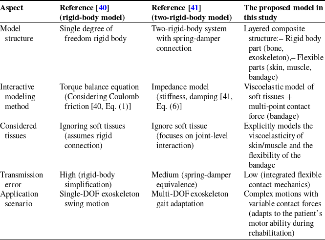
Prior studies (e.g., [Reference Tran, Cheng, Lin, Duong and Huang40, Reference Huang, Cheng, Qiu and Zhang41]) simplify the human–exoskeleton interaction interface as rigid-body or spring-damper-connected two-rigid-body systems, neglecting the mechanical properties of soft tissues (skin, muscle, and flexible bandages). In contrast, our model adopts a layered composite structure to distinguish rigid components (human bones, exoskeleton) and flexible components (soft tissues, connectors). By introducing viscoelastic parameters to characterize energy dissipation in soft tissues, we reduce transmission errors caused by oversimplification (see Table I for detailed comparisons).
Comparison of the proposed model with prior studies.

This explicit modeling of soft tissue mechanics and flexible contact interactions enables more accurate simulation of complex rehabilitation motions, surpassing the rigid-body assumptions in ref. [Reference Tran, Cheng, Lin, Duong and Huang40] (which ignore soft tissue flexibility) and the limited joint-level focus in ref. [Reference Huang, Cheng, Qiu and Zhang41] (which do not explicitly model soft tissue viscoelasticity). Our model dynamically adapts to changes in the patient’s motor ability during rehabilitation, enhancing its applicability to real-world scenarios.
As illustrated in Figure 4, the skin and muscle on the human limb surface form a flexible contact layer
 $S_{2}$
. Unlike the contact collision of two rigid bodies, the contact interface between the rehabilitation robot exoskeleton and the human body exhibits two regimes. The first regime involves the bottom support acting as the rigid exoskeleton’s
 $S_{1}$
surface. The other is
 $S_{3}$
fixed by a flexible belt. The rigid and flexible properties of “B” and “E” are different, and there is an approximate non-contact between
 $S_{1}$
and
 $S_{2}$
in the process of motion, that is,
 $z_{0}\geq 0$
; and
 $S_{3}$
is always in contact with
 $S_{2}$
, that is,
 $z_{3}\equiv 0$
. Therefore, this study treats human-limb–exoskeleton collision contact as flexible contact for modeling. Under the assumption of no collision impulse, contact loss is determined directly from position and velocity without considering impulsive dynamics. The interaction between human lower limbs and the exoskeleton is investigated in one-dimensional sagittal-plane collision contact, with other three-dimensional components neglected. Within the human–machine interaction contact system, the generated contact interaction force is dominated by contact and friction forces perpendicular to the leg direction. This study employs a first-order system to construct a flexible contact model. This modeling approach enables the separation of rigid-body dynamics in the human–machine coupled system from contact mechanics. The relative position and velocity of the human–machine system determine the contact interaction force, which is subsequently incorporated into the robot dynamics system as a known input.
Human-exoskeleton interaction contact model.

The contact model mainly includes the exoskeleton rigid body part “E,” the flexible belt part “B,” the limb skeleton rigid body “H”, the zero-mass contact surface
 $S_{1} , S_{2}$
, and
 $S_{3}$
, and three equivalent springs and three equivalent dampers. Variables
 $z_{1} , z_{2} , z_{3}$
, and
 $z_{0}$
represent the position of the
 $S_{1}$
and
 $S_{2}$
contact surfaces and the distance between the contact surfaces, respectively.
 $K_{s1}^{r},K_{s3}^{r},K_{s2}^{h},C_{s1}^{r},C_{s3}^{r},$
and
 $C_{s2}^{h}$
are the stiffness and damping coefficients of the
 $S_{1},S_{3}$
, and
 $S_{2}$
contact surfaces, respectively. As the human limb and exoskeleton contact interface are engaged via strapping, lateral friction acts on the limb in addition to the normal contact force
 $F_{f}$
.
In flexible contact modeling, the Coulomb friction model effectively characterizes the frictional force. Accounting for frictional effects, the human–robot interaction contact model (HRIF) is herein developed:
 \begin{align} F_{i}& =\left\{\begin{array}{l} K_{1}^{d}\left(v_{i}^{r}-v_{i}^{h}\right)+C_{1}^{d}\left(v_{i}^{r'}-v_{i}^{h'}\right)+f_{c,i}sign\left(v_{i}^{r'}-v_{i}^{h'}\right)+f_{s,i}\left(v_{i}^{r'}-v_{i}^{h'}\right)\!,\,\,\mathrm{z}_{0}\gt 0\\[3pt] K_{2}^{d}\left(v_{i}^{r}-v_{i}^{h}\right)+C_{2}^{d}\left(v_{i}^{r'}-v_{i}^{h'}\right)+f_{c,i}sign\left(v_{i}^{r'}-v_{i}^{h'}\right)+f_{s,i}\left(v_{i}^{r'}-v_{i}^{h'}\right)\!,\,\,\mathrm{z}_{0}=0 \end{array}\right. \nonumber\\[3pt] K_{1}^{d} &=\frac{K_{s3}^{r}K_{s2}^{h}}{K_{s3}^{r}+K_{s2}^{h}},\mathrm{C}_{1}^{d}=C_{s3}^{r}+C_{s2}^{h} \nonumber\\[3pt] K_{2}^{d} & = \frac{\left(K_{s1}^{r}+K_{s3}^{r}\right)K_{s2}^{h}}{K_{s1}^{r}+K_{s3}^{r}+K_{s2}^{h}},\mathrm{C}_{2}^{d}=\frac{C_{s1}^{r}C_{s3}^{r}}{C_{s1}^{r}+C_{s3}^{r}}+C_{s2}^{h} \end{align}
In the formula,
 $F_{i}~ ,~ i=1,2$
represent the human–machine interaction contact force at the thigh and calf, respectively.
 $v_{i}^{r},v_{i}^{h}$
represent the displacement of the exoskeleton and the human lower limb segments.
 $f_{c,i},f_{s,i}$
represent the Coulomb friction coefficient and the viscous friction coefficient, respectively.
3.4. Integrated human-exoskeleton coupling model
Analysis of the rehabilitation robot’s exoskeleton joint driving torque reveals that the joint torque output comprises three primary components: the torque required to drive the exoskeleton under ideal conditions
 $\tau _{r}$
, the torque required to drive the patient’s lower limbs under perfect conditions
 $\tau _{h}$
, and the human–machine interaction force resulting from rigid-flexible coupling losses
 $\tau _{hr}$
:
 \begin{align} \tau =\tau _{r}+\tau _{hr}+\tau _{h} \end{align}
Based on the dynamic equation of the rehabilitation robot’s exoskeleton (formula (1)), parameter identification under no-load conditions determines the unknown parameters of the exoskeleton dynamic model to derive the torque required to drive the exoskeleton. Friction at the exoskeleton’s actuated joints is influenced by multiple factors, exhibiting nonlinear dependence on joint velocity, which renders accurate linear modeling challenging. The rehabilitation robot employed in this study is equipped with a torque sensor at the joint output, enabling direct measurement of joint torque and indirect compensation for frictional interference. In subsequent control research, motor current measurements can estimate the torque output of the deactivated motor. The discrepancy between the joint’s commanded torque and measured torque reveals the torque dissipated by friction, which is temporarily disregarded in this analysis. For human lower limbs, this study adopts the anthropometric mass proportion method from Anthropometric Reference Data [Reference Fryar, Carroll, Gu, Afful and Ogden42] to determine thigh and calf mass ratios. By integrating the human lower limb equivalent dynamics equation with formula (11), the torque required to drive the limbs under ideal conditions is identified. The HRIF model characterizes human–machine coupling forces, and by transforming each component’s torque into the exoskeleton’s joint space, the human–machine coupled dynamic equation is ultimately derived:
 \begin{align} M_{r}\theta ''_{r}+C_{r}\theta '_{r}+G_{r}\theta _{r}=\tau _{r}+\tau _{hr}+\tau _{h} \\[-28pt] \nonumber \end{align}
 \begin{align} \tau _{hr}=Q_{hr}\left(C_{i}^{h},K_{i}^{h},C_{i}^{r},K_{i}^{r},f_{c,i},f_{s,i}\right) \\[-28pt] \nonumber \end{align}
 \begin{align} \tau _{h}={\unicode[Arial]{x03A6}} _{r}^{T}{\unicode[Arial]{x03A6}} _{h}^{-T}\left(M_{h}\theta ''_{h}+C_{h}\theta '_{h}+G_{h}\right) \\[-6pt] \nonumber \end{align}
In the formula,
 $Q_{hr}(\,)$
represents the function of the parameters of the interactive contact model,
 ${\unicode[Arial]{x03A6}} _{h} , {\unicode[Arial]{x03A6}} _{r}$
is the Jacobian matrix of the exoskeleton and the human lower limb.
4. Adaptive admittance control for lower limb rehabilitation robots
The patient’s active force in human–machine interaction reflects motor ability and intention [Reference Zou, Zeng, Huang, Peng, Zhang and Cheng43]. To ensure patient safety and comfort, the rehabilitation robot must adjust the mechanical leg’s trajectory control according to the patient’s motion intention. To avoid excessive compressive forces between the mechanical leg and human lower limbs – and thereby prevent injury – this study presents an adaptive admittance control strategy utilizing root mean square propagation (RMSprop) to dynamically adjust damping and stiffness parameters for compliance control.
In rehabilitation scenarios, the adaptive adjustment of admittance control parameters must simultaneously satisfy human–machine collaborative control’s safety, real-time performance, and dynamic adaptability requirements [Reference Almaghout, Tarvirdizadeh, Alipour and Hadi44]. Traditional gradient descent (SGD) with a fixed learning rate fails to address time-varying demands, while deep learning methods rely on offline training [Reference Arefeen and Xiang45]. In contrast, RMSprop achieves dynamic learning rate scaling via exponential weighted averaging of gradient squares. The parameter update process will not cause system oscillation due to energy accumulation, ensuring safety. Compared to deep learning, RMSprop’s low computational complexity meets the real-time constraint of the rehabilitation robot’s 1-ms joint control cycle. Furthermore, as patients’ motor function evolves during rehabilitation (e.g., joint angular velocity increasing from 0.1 rad/s to 0.8 rad/s), RMSprop’s adaptive mechanism, via adjustable exponential weighting coefficients, flexibly balances historical and current gradients, enabling personalized adaptation to non-stationary force distributions [Reference Rospawan, Tsai and Hung46]. Thus, RMSprop is selected as the adaptive adjustment algorithm for admittance control parameters.
In this study, the human–machine interaction force deviation is defined as a loss function, serving as a metric to evaluate human–machine interaction performance:
 \begin{align} {\unicode[Arial]{x0393}} \left(t\right)=\left\| F^{m}\left(t\right)-F_{d}\left(t\right)\right\| _{2} \end{align}
where
 $F^{m}$
and
 $F_{d}$
are the measured and expected values of the human–-exoskeleton interaction force. The damping parameter learning rate is defined as follows:
 \begin{align} G_{B}^{m}=\gamma G_{B}^{m-1}+\left(1-\gamma \right)\cdot \left[\frac{\partial {\unicode[Arial]{x0393}} ^{m}\left(t\right)}{\partial B_{d}^{m}\left(t\right)}\right]^{2} \end{align}
The adaptive adjustment rate of the damping coefficient is derived:
 \begin{align} B_{d}^{m+1}\left(t\right)=B_{d}^{m}\left(t\right)-\frac{\eta _{B}}{\sqrt{G_{B}^{m}+\varepsilon }}\cdot \frac{\partial {\unicode[Arial]{x0393}} ^{m}\left(t\right)}{\partial B_{d}^{m}\left(t\right)} \end{align}
where
 $\gamma$
represents the attenuation coefficient,
 $\eta$
represents the learning rate,
 $\varepsilon$
represents the numerical stability of the small constant,
 $\partial {\unicode[Arial]{x0393}} ^{m}(t)/\partial B_{d}^{m}(t)$
the calculation formula is
 \begin{align} \frac{\partial {\unicode[Arial]{x0393}} ^{m}\left(t\right)}{\partial B_{d}^{m}\left(t\right)}=\frac{\partial f^{m}\left(t\right)}{\partial B_{d}^{m}\left(t\right)}\cdot \frac{\partial {\unicode[Arial]{x0393}} ^{m}\left(t\right)}{\partial f^{m}\left(t\right)}=\theta '^{m}\left(t\right)\frac{\partial {\unicode[Arial]{x0393}} ^{m}\left(t\right)}{\partial F^{m}\left(t\right)} \end{align}
Similarly, the learning rate and adaptive adjustment rate of the stiffness coefficient are derived:
 \begin{align} G_{K}^{m}=\gamma G_{K}^{m-1}+\left(1-\gamma \right)\cdot \left[\frac{\partial {\unicode[Arial]{x0393}} ^{m}\left(t\right)}{\partial K_{d}^{m}\left(t\right)}\right]^{2} \end{align}
 \begin{align} K_{d}^{m+1}\left(t\right)=K_{d}^{m}\left(t\right)-\frac{\eta _{K}}{\sqrt{G_{K}^{m}+\varepsilon }}\cdot \frac{\partial {\unicode[Arial]{x0393}} ^{m}\left(t\right)}{\partial K_{d}^{m}\left(t\right)} \end{align}
 \begin{align} \frac{\partial {\unicode[Arial]{x0393}} ^{m}\left(t\right)}{\partial K_{d}^{m}\left(t\right)}=\frac{\partial f^{m}\left(t\right)}{\partial K_{d}^{m}\left(t\right)}\frac{\partial {\unicode[Arial]{x0393}} ^{m}\left(t\right)}{\partial f^{m}\left(t\right)}=\theta ^{m}\left(t\right)\frac{\partial {\unicode[Arial]{x0393}} ^{m}\left(t\right)}{\partial F^{m}\left(t\right)} \\[-12pt] \nonumber \end{align}
Formula (12) quantifies the human–machine contact relationship, maps it to joint space, and establishes the mechanical impedance relationship during human–machine interaction as
 \begin{align} f\left(t\right)=M\left(t\right)\theta ''\left(t\right)+B\left(t\right)\theta '\left(t\right)+K\left(t\right)\theta \left(t\right) \end{align}
To obtain
 $\partial {\unicode[Arial]{x0393}} /\partial F_{d}^{m}(t)$
, the idea of iterative learning is used to calculate [Reference Li and Ge47]. The admittance system assumes that the human–machine interaction force in the initial static state is 0. On this basis, the state variables
 $x_{1}(t)=\theta (t) , x_{2}(t)=x'_{1}(t) , x'_{3}(t)=f(t)$
are taken. The output matrix between the system state and the output
 $y(t)$
is
 $C(t)$
, and the direct transfer matrix is
 $D(t)$
. The human–machine interaction force is treated as the system input. The state-space expression and output equation for the mechanical impedance in human–machine interaction are given as follows:
 \begin{align} \left\{\begin{array}{c} x'\left(t\right)=A\left(t\right)x\left(t\right)+B\left(t\right)f\left(t\right)\\[3pt] y\left(t\right)=C\left(t\right)x\left(t\right)+D\left(t\right)f\left(t\right) \end{array}\right. \end{align}
In the formula,
 $A(t)$
is the state matrix,
 $B(t)$
is the input matrix, and its specific form is
 \begin{align} A\left(t\right)=\left[\begin{array}{l@{\quad}l@{\quad}l} 0 & 1 & 0\\[3pt] -M^{-1}\left(t\right)K\left(t\right) & -M^{-1}\left(t\right)B\left(t\right) & 0\\[3pt] 0 & 0 & 0 \end{array}\right] \\[-24pt] \nonumber \end{align}
 \begin{align} B\left(t\right)=\left[\begin{array}{l} 0\\[3pt] M^{-1}\left(t\right)\\[3pt] 1 \end{array}\right] \\[-24pt] \nonumber \end{align}
 \begin{align} x\left(t\right)=\left[\begin{array}{l} x_{1}\left(t\right)\\[3pt] x_{2}\left(t\right)\\[3pt] x_{3}\left(t\right) \end{array}\right] \\[-12pt] \nonumber \end{align}
Taking
 $f(t)$
as the control input, for the linear time-invariant system described by Eq. (25), the D-type learning control mechanism is adopted, and the update rule of human–machine interaction force is
 \begin{align} f^{m}\left(t\right)=f^{m-1}\left(t\right)-\varsigma e_{m}\left(t\right) \end{align}
In the formula,
 $e_{m}(t)=y'^{m}(t)-y'_{d}(t) , \varsigma$
satisfies:
 \begin{align} \left\| I-\varsigma B\left(t\right)C\left(t\right)\right\| _{\infty }\lt 1 \end{align}
where
 $I$
is the identity matrix.
By updating the control input, that is, the interaction force, the deviation between the control output
 $y^{m}(t)$
and
 $y_{d}(t)$
is reduced. The deviation is also described by the loss function of Eq. (17), and it can be obtained:
 \begin{align} f^{m}\left(t\right)=f^{m}\left(t\right)-\sigma \cdot \frac{\partial {\unicode[Arial]{x0393}} ^{m}\left(t\right)}{\partial F^{m}\left(t\right)} \end{align}
By formulas (30) and (31), we obtain:
 \begin{align} \frac{\partial {\unicode[Arial]{x0393}} ^{m}\left(t\right)}{\partial F^{m}\left(t\right)}=\frac{\varsigma }{\sigma }\left(y'^{m}\left(t\right)-y'_{d}\left(t\right)\right) \end{align}
By substituting formula (32) into formula (19) and formula (22), and taking
 $\alpha =\varsigma /\sigma$
, the adaptive rate of the damping coefficient and stiffness coefficient can be obtained:
 \begin{align} B_{d}^{m+1}\left(t\right)=B_{d}^{m}\left(t\right)-\frac{\eta _{B}\alpha \theta '^{m}\left(t\right)}{\sqrt{G_{B}^{m}+\varepsilon }}\cdot \left(y'^{m}\left(t\right)-y'_{d}\left(t\right)\right) \end{align}
 \begin{align} K_{d}^{m+1}\left(t\right)=K_{d}^{m}\left(t\right)-\frac{\eta _{K}\alpha \theta ^{m}\left(t\right)}{\sqrt{G_{K}^{m}+\varepsilon }}\cdot \left(y'^{m}\left(t\right)-y'_{d}\left(t\right)\right) \\[9pt] \nonumber \end{align}
The inner-loop position controller is integrated with the outer-loop admittance controller. RMSprop is employed to optimize the admittance parameters, and the adaptive adjustment rates of the admittance controller’s damping and stiffness parameters are designed to achieve human–machine cooperative motion control via interaction force. The framework of the double-loop control system is illustrated in Figure 5.
Adaptive admittance control system framework.

5. Experiment validation
5.1. Experimental identification of exoskeleton inertial parameters
The rehabilitation robot’s exoskeleton model can be identified via conventional dynamic parameter identification following linearization. Linearization of the exoskeleton dynamic equation enables the derivation of rigid exoskeleton parameters. The linearized form of the dynamic equation is
 \begin{align} \tau _{r}=M_{r}\theta ''_{r}+C_{r}\theta '_{r}+G_{r}=H\left(\theta ''_{r},\theta '_{r},\theta _{r}\right)X \end{align}
where
 $H(\theta ''_{r},\theta '_{r},\theta _{r})$
is the observation matrix and
 $X$
is the inertial parameter matrix. A detailed explanation is given in the Appendix.
Under the no-load condition (i.e., considering only the exoskeleton’s weight), the exoskeleton’s motion excitation trajectory is input to the rehabilitation robot. This trajectory is parameterized using the FFS method [Reference Losantos, Montiel, Mustata, Zorrilla and Valiño48] and optimized using the condition number criterion [Reference Ostaszewicz and Rogowski49] and the particle swarm optimization algorithm [Reference Suraj, Wu, Guru and Buyya50]. The trajectory covers the rehabilitation training range of the hip joint (−30°, 60°) and knee joint (0°, 120°), ensuring effective excitation of the inertial parameters to be identified.
The high-precision MILLE encoder (6400 PPR) and torque sensor (range: 360 N m, resolution: 0.01 N m) were used. They collected data from the rehabilitation robot operating along the motion excitation trajectory, including hip and knee joint angles and joint output torque. The collected data were first smoothed and filtered to ensure data accuracy and reliability. The LOWESS method was employed for filtering, with the window size control parameter span set to 0.05, which preserved key motion features while suppressing noise.
The genetic algorithm [Reference Losantos, Montiel, Mustata, Zorrilla and Valiño48, Reference Ostaszewicz and Rogowski49] was used to identify the inertial parameters. The relevant parameter settings were as follows: the initial population size was 1000 (with the optimal size determined via pre-test), the crossover probability was 0.8 (determined by referring to similar studies and adapted to the present model), the mutation probability was 0.01 (to balance convergence and diversity), and the maximum number of iterations was 1000 (pre-test verified the sufficiency of convergence). The static penalty function was used to constrain the reasonable range of the parameters to be identified. The objective function was the minimum of the error between the theoretical and measured torque, plus the minimum of the static penalty function.
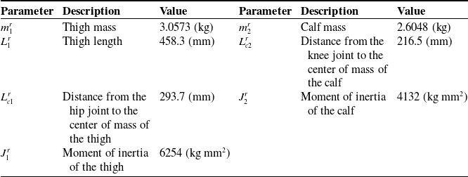
Measurement data from 10 groups of excitation trajectory motions were recorded. Each group of trajectories differed in motion amplitude, frequency, or joint coupling relationship, thus covering richer motion modes and improving the robustness of parameter identification. The dynamic inertial parameter identification results for the rehabilitation robot’s exoskeleton are shown in Table II.
Identification results of the exoskeleton.

With experimental baseline conditions unchanged, an exoskeleton motion trajectory is replanned based on the gait trajectory of healthy subjects and applied to the rehabilitation robot. Motion and torque data are collected from joint sensors. Concurrently, the theoretically determined model is employed for computation, and experimental values are compared with theoretical predictions. As shown in Figure 6, the predicted results are consistent with the overall trend of the sensor measurement results, but the measured values are greater than the expected values. To clarify the source of error, a zero-calibration test of the sensor was conducted before the experiment, and factors such as sensor accuracy and signal transmission interference were examined. It was determined that the offset arose from the sensor’s zero offset. The correlation coefficients between the measured and theoretical values were further calculated to be 0.92, indicating a high correlation between the fluctuation patterns of the two, with no impact on the validity of the verification results.
Comparison of theoretical and experimental torque results for hip and knee joints. (a) Hip joint. (b) Knee joint.

5.2. Experimental identification of human lower limb inertial parameters
The standard human body attribute proportion method described in ref. [Reference Fryar, Carroll, Gu, Afful and Ogden42] is a generic empirical model. However, due to individual differences in anthropometric parameters and body segment properties (such as height, body weight, segmental bone lengths (e.g., femur, tibia, and humerus), mass distribution, muscle-fat ratio, joint morphology, and kinematic properties), significant errors may occur. OpenSim [Reference Rajagopal, Dembia, DeMers, Delp, Hicks and Delp51], a widely used biomechanical simulation software, performs inverse dynamics simulations of human walking using motion data and ground reaction forces. Its accuracy is highly validated in the literature and is widely recognized for reliability [Reference Arnold, Salinas, Hakawa and Delp52, Reference Sandbakk, Dembia, Silder, Uchida, Hicks and Delp53].
Therefore, this paper collected the subject’s motion capture marker and plantar pressure data. The collected data were filtered using a Butterworth low-pass filter (cutoff frequency: 6 Hz). The generic model was scaled in OpenSim based on the filtered marker data. The collected marker data included static data used to scale the generic model and adjust its proportions to match the subject’s body dimensions and motion data used to solve inverse kinematics and inverse dynamics. By comparing the distances between the marker points of the generic model and those of the subject, the scaling ratio weights were adjusted, with the maximum error controlled to less than 2 cm and the root mean square error to less than 1 cm, thereby establishing the subject-specific model.
Then, using OpenSim’s inverse kinematics and inverse dynamics analysis functions [Reference Wei, Zhang and Zhang54], the collected plantar pressure data were loaded to calculate the muscle force, joint force, and torque of the human lower limb model. Hip and knee joint angles (flexion–extension direction time series) and joint torque (torque time series) were exported from OpenSim, while body segment parameters (such as thigh mass, moment of inertia, centroid position, among others) following model scaling were derived. The obtained joint angle and torque data were used to extract the effective segment of the walking cycle (single support phase) for subsequent parameter identification; the segment parameters were compared with the anthropometric database [Reference Winter55] to verify that parameters such as thigh moment of inertia fell within the normal biomechanical range, ensuring the model’s validity.
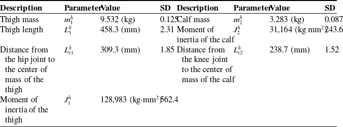
Finally, based on the joint torque and joint angle data, the least squares method was used to identify the parameters of the human lower limb dynamic model. The covariance matrix of the output parameters was obtained during the identification process. By taking the square roots of the diagonal elements of the matrix, the standard deviation (SD) of each inertial parameter was derived, quantifying the uncertainty in the parameter estimation (a smaller SD indicates better stability of the model fit to the experimental data). The detailed implementation procedure is illustrated in Figure 7, with the identification results tabulated in Table III.
Parameter identification workflow for the human lower extremity using OpenSim.

Identification results of the human lower limb.

5.3. Parameter identification of the human–machine interaction contact model
Drawing on the parameter identification framework in ref. [Reference Yan, Chen, Huang, Chen and Guo56] and other related studies, the experiment was designed based on the contact characteristics addressed in this study, and the experiment was conducted using the multi-posture lower limb rehabilitation robot platform. The subject was a 26-year-old healthy adult male, with a height of 170 cm and a weight of 66 kg. The subject’s hip and knee joints were well matched with the mechanical leg. A one-dimensional force sensor was installed at the human–machine interaction contact module of the thigh and calf (i.e., at the connection between S1 and the exoskeleton E). The sensor parameters are as follows: range: 360 N, resolution: 0.01 N, nonlinearity: ±0.02% F.S, repeatability: ±0.02% F.S, and hysteresis: ±0.02% F.S. The rehabilitation robot adopted a passive training mode to drive the subject to move along the preset gait trajectory. The subject did not actively exert force; instead, the mechanical leg drove the human lower limbs to simulate human–machine interaction in real rehabilitation scenarios.
Reflective markers were attached to the subject’s lower limbs and mechanical legs, and the NOKOV motion capture system was used to acquire real-time motion information of the human limbs and the rehabilitation robot exoskeleton (sampling frequency: 100 Hz). Motion and interaction contact force information were recorded synchronously during the experiment. A total of 10 sets of data were collected, with the first eight sets used as the experimental group (for parameter identification) and the last two sets as the verification group (for model verification). The LOWESS method was first used for filtering, with the window size control parameter span set to 0.05, which preserved key motion features and suppressed noise.
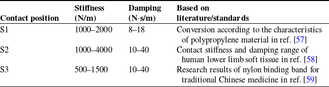
The ranges of the model’s three equivalent spring and damping coefficients are determined based on their material properties and related research, as presented in Table IV. Among them, S1 (polypropylene medical guard plate) is a hard material with small deformation and a narrow parameter variation range. S2 (human tissue), composed of soft structures such as muscle and skin, exhibits significant deformation and slow recovery after loading, resulting in a wide damping parameter range. The elasticity of S3 (flexible strap, nylon material) is between that of the first two; it can be stretched but has a limited deformation range.
Reference range of parameters of the interactive contact model.

To address the complexity of the human–machine interaction contact model and account for the overall context, this study uses the genetic algorithm – suitable for nonlinear and multi-parameter optimization problems – to identify the parameters of the human–machine interaction contact model. The relevant parameters are set as follows: initial population size = 500, crossover probability = 0.8, mutation probability = 0.02, constraint conditions are set according to the previously determined parameter ranges, and maximum number of iterations = 1000 (convergence criterion: fitness change<1e-4 for 50 consecutive generations). The objective function is the minimum error between the theoretical and measured interaction forces.
The identification results of the three equivalent springs and damping coefficients are presented in Table V. These results were verified using data from the verification group. Figure 8 shows the verification group’s model prediction and actual measurement results over two random motion cycles. By comparing the force–time curves of the theoretical and measured results in the figure, the two trends are found to be generally consistent. The maximum root mean square errors (RMSEs) of the verification results for the thigh and calf are 2.3187 and 1.4461 N, respectively. This error range falls within the valid error range of similar research results (RMSE/maximum interaction force ≤ 10%, ref. [Reference Yan, Chen, Huang, Chen and Guo56]), confirming the validity of the identification results.
Parameter identification results of the interactive contact model.

Validation of human–computer interaction contact model parameter results.

5.4. Experimental validation of adaptive admittance control
Based on the results of the previous parameter identification experiments, the numerical solution of the human–machine coupled dynamic equation excluding interaction losses is derived. The interaction force is then fed into the adaptive admittance control model to obtain trajectory deviations induced by interaction forces. To validate the control performance and interaction comfort of human–machine cooperative motion with the adaptive admittance controller, a comparative experiment is designed in this study.
Subjects were secured to the rehabilitation robot and walked at a constant speed on a treadmill. The NOKOV motion capture system collected human lower limb motion data, while the rehabilitation robot synchronously recorded exoskeleton joint trajectory outputs and interaction forces.
Figure 9 illustrates the hip and knee joint motion trajectories and human–machine interaction forces under adaptive admittance parameter adjustment. Figure 10 depicts the same metrics with fixed admittance parameters. Figures 9 and 10 show four complete and continuous gait cycles [Reference Yin, Zhu, Gao, Niu, Shen, Fan and Wang60] randomly selected during walking.
Experimental results of the adaptive admittance controller.

Experimental results of the fixed admittance controller.

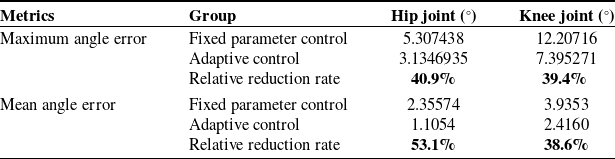
Comparison of joint angle errors.

The use of boldface is to precisely emphasize the relative improvement effects of adaptive control on two types of metrics (joint angle errors and human - exoskeleton interaction forces).
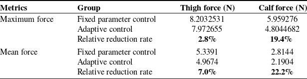
Comparison of human-exoskeleton interaction forces.

The use of boldface is to precisely emphasize the relative improvement effects of adaptive control on two types of metrics (joint angle errors and human - exoskeleton interaction forces).
The experimental data comparisons are presented in Tables VI and VII. The relative reduction rate is calculated as
 \begin{align} \text{Relative reduction rate}=\left(1-\frac{\text{Adaptive}}{\text{Fixed}}\right)\times 100 \end{align}
Table VI demonstrates that the adaptive controller reduces the maximum hip and knee joint angle errors by 40.9% and 39.4%, respectively, and mean angle errors by 53.1% and 38.6% compared to the fixed parameter controller. For human–exoskeleton interaction forces (Table VII), the maximum thigh and calf forces decrease by 2.8% and 19.4%, while mean forces reduce by 7.0% and 22.2%. These results confirm the adaptive controller’s superiority in improving joint angle consistency and minimizing interaction forces, with clear baseline comparisons (fixed parameter controller) provided for each metric.
6. Conclusion
This study presents a multi-posture lower limb rehabilitation robot system designed to address multi-stage rehabilitation requirements. By analyzing human–machine coupling interactions during rehabilitation training, the human–machine contact relationship is quantified using a flexible contact approach, enabling dynamic decoupling of interaction forces and motion trajectory deviations. Unlike conventional human–machine integrated equivalent modeling approaches, the human–machine system is decomposed into subsystems, and a human–machine coupled dynamic model accounting for contact losses in human–machine interaction is developed.
An admittance controller incorporating adaptive RMSprop rate adjustment is developed. Leveraging a low-level position controller, a double-loop control system for the lower limb rehabilitation robot is designed to realize adaptive compliance control.
The inertial parameters of the exoskeleton of the lower-limb rehabilitation robot and the human lower limb were identified through experiments. The inertial and contact model parameters of each human–machine system component were determined. A comparative experiment was conducted to verify the adaptive compliance controller. The results show that, compared with the fixed-compliance-parameter controller, the adaptive compliance controller significantly improves trajectory consistency, with the maximum joint angle error reduced by more than 48.4% and the maximum human–machine interaction force decreased by more than 21.4%. This advantage directly enhances the safety and effectiveness of rehabilitation training. The notable reduction in trajectory error can mitigate the risk of secondary injury caused by movement deviation. At the same time, the decrease in interaction force can improve patients’ training adaptability and ensure safety during long-term rehabilitation.
Compared with the research by Lu et al. [Reference Lu19], this study further elucidates the mechanism of human–machine interaction contact in lower-limb rehabilitation training and provides new insights for reducing human–machine interaction force, enhancing comfort and coordination, and mitigating the risk of secondary injury. Compared with existing fixed-parameter control [Reference Chen, Wang, Song, Wang, Zhang and Li31] or simplified human–machine models [Reference Huang, Cheng, Qiu and Zhang41], the “human–machine coupling dynamic model considering contact loss” proposed in this study overcomes the limitations of traditional integrated modeling and achieves dynamic decoupling of force and trajectory deviation. The “adaptive root mean square propagation rate adjustment admittance controller” developed based on this model addresses the static setting of compliance parameters and enables dynamic and personalized rehabilitation control. The above results provide key technical support for rehabilitation robots’ human–machine collaboration theory and advance the field from “passive assistance” to “active adaptation”.
However, there are three key limitations in this study:
-
1. Limitation in subject scope: The methods were validated only in healthy adults, and their efficacy for stroke patients with motor dysfunctions (e.g., spastic hemiplegia, balance disorders) remains untested. Pathological individual differences (e.g., muscle spasticity, joint contracture) may disrupt the controller’s ability to adapt to dynamic human–machine interaction patterns, affecting control strategies’ adaptability in clinical use.
-
2. Limitation in algorithm robustness evaluation: While effective in standard scenarios, the controller’s robustness under extreme conditions (sudden patient resistance, external disturbances) has not been tested. This unevaluated robustness may lead to inadequate real-time adjustment under such conditions, potentially limiting its real-time adaptability in practice.
-
3. Insufficiency in clinical validation: The evaluation focused on kinematic and force interaction metrics but lacked a systematic assessment of long-term outcomes (motor function recovery, gait symmetry, and quality of life). These long-term outcomes are critical for determining the practical clinical utility of the methods, as they directly reflect the actual benefits for rehabilitation.
In the future, clinical trials for different patient cohorts, algorithm optimization, and long-term efficacy tracking can be conducted to address the above limitations. On this basis, the human–machine coupling dynamics modeling and adaptive compliance control method proposed in this study can be extended to other fields of wearable robots, such as exoskeleton assistance devices and robots for individuals with disabilities, and provide a general technical framework for solving safety and comfort issues in human–machine collaboration.
Author contribution
Conceptualization, Chao Gao and Chang Wang; methodology, Chao Gao; software, Chao Gao; validation, Chang Wang, Hui Li, Jianhua Zhang, Xinpeng Du, and Jianjun Zhang; formal analysis, Chang Wang; investigation, Hui Li; resources, Xinpeng Du; data curation, Jianhua Zhang; writing—original draft preparation, Chao Gao; writing—review and editing, Chang Wang; visualization, Chang Wang; supervision, Jianhua Zhang; project administration, Jianjun Zhang; funding acquisition, Hui Li.
Financial support
This work was supported by the National Natural Science Foundation of National Key R&D Program of China (Grant No. 2023YFB4706100) and National Natural Science Foundation of China (Grant No. U23A20338).
Competing interests
The authors declare no conflicts of interest exist.
Ethical approval
Not applicable.
Appendix
 \begin{align} \begin{array}{l} \left\{\begin{array}{l} x_{c1}^{r}=L_{c1}^{r}\sin \theta _{1}^{r}\\[3pt] y_{c1}^{r}=L_{c1}^{r}\cos \theta _{1}^{r} \end{array}\right.\\[3pt] \left\{\begin{array}{l} x_{c2}^{r}=L_{1}\sin \theta _{1}^{r}+L_{c2}^{r}\sin \left(\theta _{1}^{r}+\theta _{2}^{r}\right)\\[3pt] y_{c2}^{r}=L_{1}\cos \theta _{1}^{r}+L_{c2}^{r}\cos \left(\theta _{1}^{r}+\theta _{2}^{r}\right) \end{array}\right. \end{array} \\[-24pt] \nonumber \end{align}
 \begin{align} \begin{array}{l} \left\{\begin{array}{l} x_{c1}^{r'}=L_{c1}^{r}\cos \theta _{1}^{r}\cdot \theta _{1}^{r'}\\[3pt] y_{c1}^{r'}=-L_{c1}^{r}\sin \theta _{1}^{r}\cdot \theta _{1}^{r'} \end{array}\right.\\[3pt] \left\{\begin{array}{l} x_{c2}^{r'}=L_{1}\cos \theta _{1}^{r}\cdot \theta _{1}^{r'}+L_{c2}^{r}\cos \left(\theta _{1}^{r}+\theta _{2}^{r}\right)\cdot \left(\theta _{1}^{r'}+\theta _{2}^{r'}\right)\\[3pt] y_{c2}^{r'}=-L_{1}\sin \theta _{1}^{r}\cdot \theta _{1}^{r'}-L_{c2}^{r}\sin \left(\theta _{1}^{r}+\theta _{2}^{r}\right)\cdot \left(\theta _{1}^{r'}+\theta _{2}^{r'}\right) \end{array}\right. \end{array} \\[-24pt] \nonumber \end{align}
 \begin{align} \begin{array}{l} M_{11}^{r}=m_{1}^{r}\left(L_{c1}^{r}\right)^{2}+m_{2}^{r}\left(L_{c2}^{r}\right)^{2}+m_{2}^{r}\left(L_{1}\right)^{2}+2m_{2}^{r}L_{1}L_{c2}^{r}\cos \left(2\theta _{1}^{r}+\theta _{2}^{r}\right)+J_{1}^{r};\\[3pt] M_{12}^{r}=m_{2}^{r}\left(L_{c2}^{r}\right)^{2}+m_{2}^{r}L_{1}L_{c2}^{r}\cos \left(2\theta _{1}^{r}+\theta _{2}^{r}\right);\\[3pt] M_{21}^{r}=m_{2}^{r}\left(L_{c2}^{r}\right)^{2}+m_{2}^{r}L_{1}L_{c2}^{r}\cos \left(2\theta _{1}^{r}+\theta _{2}^{r}\right);\\[3pt] M_{22}^{r}=m_{2}^{r}\left(L_{c2}^{r}\right)^{2}+J_{2}^{r}; C_{11}^{r}=0; C_{12}^{r}=-m_{2}^{r}L_{1}L_{c2}^{r}\sin \theta _{1}^{r};\\[3pt] C_{21}^{r}=m_{2}^{r}L_{1}L_{c2}^{r}\sin \theta _{2}^{r}; C_{22}^{r}=0; D_{11}^{r}=-2m_{2}^{r}L_{1}L_{c2}^{r}\sin \theta _{1}^{r};\\[3pt] D_{12}^{r}=D_{21}^{r}=D_{22}^{r}=0; G_{2}^{r}=-m_{2}^{r}gL_{c2}^{r}\sin \left(\theta _{1}^{r}+\theta _{2}^{r}\right);\\[3pt] G_{1}^{r}=-m_{1}^{r}gL_{c1}^{r}\sin \theta _{1}^{r}-m_{2}^{r}gL_{c2}^{r}\sin \left(\theta _{1}^{r}+\theta _{2}^{r}\right)-m_{2}^{r}gL_{1}\sin \theta _{1}^{r};\\[3pt] J_{c1}^{r}=I_{z1}^{r}+I_{z2}^{r}+m_{1}^{r}\left(L_{c1}^{r}\right)^{2}+m_{2}^{r}\left(L_{c2}^{r}\right)^{2}+m_{2}^{r}\left(L_{1}^{r}\right)^{2};\\[3pt] J_{c2}^{r}=I_{z2}^{r}+m_{2}^{r}\left(L_{c2}^{r}\right)^{2}; \end{array} \\[-24pt] \nonumber \end{align}
 \begin{align} \begin{array}{l} \left\{\begin{array}{l} x_{c1}^{h}=L_{c1}^{h}\sin \theta _{1}^{h}\\[3pt] y_{c1}^{h}=L_{c1}^{h}\cos \theta _{1}^{h} \end{array}\right.\\[3pt] \left\{\begin{array}{l} x_{c2}^{h}=L_{1}\sin \theta _{1}^{h}+L_{c2}^{h}\sin \left(\theta _{1}^{h}+\theta _{2}^{h}\right)\\[3pt] y_{c2}^{h}=L_{1}\cos \theta _{1}^{h}+L_{c2}^{h}\cos \left(\theta _{1}^{h}+\theta _{2}^{h}\right) \end{array}\right. \end{array} \\[-24pt] \nonumber \end{align}
 \begin{align} \begin{array}{l} \left\{\begin{array}{l} x_{c1}^{h'}=L_{c1}^{h}\cos \theta _{1}^{h}\cdot \theta _{1}^{h'}\\[3pt] y_{c1}^{h'}=-L_{c1}^{h}\sin \theta _{1}^{h}\cdot \theta _{1}^{h'} \end{array}\right.\\[3pt] \left\{\begin{array}{l} x_{c2}^{h'}=L_{1}\cos \theta _{1}^{h}\cdot \theta _{1}^{h'}+L_{c2}^{h}\cos \left(\theta _{1}^{h}+\theta _{2}^{h}\right)\cdot \left(\theta _{1}^{h'}+\theta _{2}^{h'}\right)\\[3pt] y_{c2}^{h'}=-L_{1}\sin \theta _{1}^{h}\cdot \theta _{1}^{h'}-L_{c2}^{h}\sin \left(\theta _{1}^{h}+\theta _{2}^{h}\right)\cdot \left(\theta _{1}^{h'}+\theta _{2}^{h'}\right) \end{array}\right. \end{array} \\[-24pt] \nonumber \end{align}
 \begin{align} \begin{array}{l} M_{11}^{h}=m_{1}^{h}\left(L_{c1}^{h}\right)^{2}+m_{2}^{h}\left(L_{c2}^{h}\right)^{2}+m_{2}^{h}\left(L_{1}\right)^{2}+2m_{2}^{h}L_{1}L_{c2}^{h}\cos \left(2\theta _{1}^{h}+\theta _{2}^{h}\right)+J_{1}^{h};\\[3pt] M_{12}^{h}=m_{2}^{h}\left(L_{c2}^{h}\right)^{2}+m_{2}^{h}L_{1}L_{c2}^{h}\cos \left(2\theta _{1}^{h}+\theta _{2}^{h}\right);\\[3pt] M_{21}^{h}=m_{2}^{h}\left(L_{c2}^{h}\right)^{2}+m_{2}^{h}L_{1}L_{c2}^{h}\cos \left(2\theta _{1}^{h}+\theta _{2}^{h}\right);\\[3pt] M_{22}^{h}=m_{2}^{h}\left(L_{c2}^{h}\right)^{2}+J_{2}^{h}; C_{11}^{h}=0; C_{12}^{h}=-m_{2}^{h}L_{1}L_{c2}^{h}\sin \theta _{1}^{h};\\[3pt] C_{21}^{h}=m_{2}^{h}L_{1}L_{c2}^{h}\sin \theta _{2}^{h}; C_{22}^{h}=0; D_{11}^{h}=-2m_{2}^{h}L_{1}L_{c2}^{h}\sin \theta _{1}^{h};\\[3pt] D_{12}^{h}=D_{21}^{h}=D_{22}^{h}=0; G_{2}^{h}=-m_{2}^{h}gL_{c2}^{h}\sin \left(\theta _{1}^{h}+\theta _{2}^{h}\right);\\[3pt] G_{1}^{h}=-m_{1}^{h}gL_{c1}^{h}\sin \theta _{1}^{h}-m_{2}^{h}gL_{c2}^{h}\sin \left(\theta _{1}^{h}+\theta _{2}^{h}\right)-m_{2}^{h}gL_{1}\sin \theta _{1}^{h};\\[3pt] J_{c1}^{h}=I_{z1}^{h}+I_{z2}^{h}+m_{1}^{h}\left(L_{c1}^{h}\right)^{2}+m_{2}^{h}\left(L_{c2}^{h}\right)^{2}+m_{2}^{h}\left(L_{1}^{h}\right)^{2};\\[3pt] J_{c2}^{h}=I_{z2}^{h}+m_{2}^{h}\left(L_{c2}^{h}\right)^{2}; \end{array} \\[-12pt] \nonumber \end{align}
where
 $I_{z1}^{h},I_{z2}^{h},I_{z1}^{r},$
and
 $I_{z2}^{r}$
are the rotational inertias of the thigh segment of the human lower limb about the hip joint, the thigh segment of the exoskeleton about the hip joint, the calf segment of the human lower limb about the knee joint, and the calf segment of the exoskeleton about the knee joint, respectively.
 \begin{align} {\unicode[Arial]{x03A6}} ^{j}=\left[\begin{array}{l@{\quad}l} -L_{1}^{j}\sin \left(\theta _{1}^{j}\right)-L_{2}^{j}\sin \left(\theta _{1}^{j}+\theta _{1}^{j}\right) & -L_{2}^{j}\sin \left(\theta _{1}^{j}+\theta _{1}^{j}\right)\\[3pt] L_{1}^{j}\cos \left(\theta _{1}^{j}\right)+L_{2}^{j}\cos \left(\theta _{1}^{j}+\theta _{1}^{j}\right) & L_{2}^{j}\cos \left(\theta _{1}^{j}+\theta _{1}^{j}\right) \end{array}\right] \\[-24pt] \nonumber \end{align}
 \begin{align} H=\left[\begin{array}{l@{\quad}l@{\quad}l@{\quad}l@{\quad}l@{\quad}l@{\quad}l@{\quad}l@{\quad}l@{\quad}l} H_{11} & H_{12} & H_{13} & H_{14} & H_{15} & H_{16} & H_{17} & H_{18} & H_{19} & H_{10}\\[3pt] H_{21} & H_{22} & H_{23} & H_{24} & H_{25} & H_{26} & H_{27} & H_{28} & H_{29} & H_{20} \end{array}\right] \\[-24pt] \nonumber \end{align}
 \begin{align} \begin{array}{l} H_{11}=\theta _{1}^{j''}; H_{12}=\cos \left(2\theta _{1}^{j}+\theta _{2}^{j}\right)\theta _{1}^{j''}; H_{13}=\theta _{2}^{j''};~ \\[3pt] ~ H_{14}=\cos \left(2\theta _{1}^{j}+\theta _{2}^{j}\right)\theta _{2}^{j''};H_{15}=\left(\theta _{1}^{j'}\right)^{2}; H_{16}=\sin \left(\theta _{1}^{j}\right)\left(\theta _{2}^{j'}\right)^{2}; \\[3pt] H_{17}=H_{18}=\theta _{1}^{j'}\theta _{2}^{j'}; H_{19}=g\sin \left(\theta _{1}^{j}\right);H_{10}=g\sin \left(\theta _{1}^{j}+\theta _{2}^{j}\right); \\[3pt] H_{21}=\theta _{1}^{j''}; H_{22}=\theta _{1}^{j''}\cos \left(2\theta _{1}^{j}+\theta _{2}^{j}\right); H_{23}=\theta _{1}^{j''};\\[3pt] H_{24}=\left(\theta _{1}^{j'}\right)^{2}\sin \left(\theta _{2}^{j}\right); H_{25}=\left(\theta _{1}^{j'}\right)^{2}; H_{26}=H_{27}=\theta _{1}^{j'}\theta _{2}^{j'};~ \\[3pt] ~ H_{27}=\sin \left(\theta _{2}^{j}\right)\left(\theta _{1}^{j'}\right)^{2}; H_{28}=g\sin \left(\theta _{1}^{j}+\theta _{2}^{j}\right); H_{29}=H_{20}=0; \end{array} \\[-24pt] \nonumber \end{align}
 \begin{align} X=\left[\begin{array}{l@{\quad}l@{\quad}l@{\quad}l@{\quad}l@{\quad}l@{\quad}l@{\quad}l@{\quad}l@{\quad}l} X_{11} & X_{12} & X_{13} & X_{14} & X_{15} & X_{16} & X_{17} & X_{18} & X_{19} & X_{10}\\[3pt] X_{21} & X_{22} & X_{23} & X_{24} & X_{25} & X_{26} & X_{27} & X_{28} & X_{29} & X_{20} \end{array}\right]^{T} \\[-24pt] \nonumber \end{align}
 \begin{align} \begin{array}{l} X_{11}=m_{1}^{j}\left(L_{c1}^{j}\right)^{2}+m_{2}^{j}\left(L_{c2}^{j}\right)^{2}+m_{2}^{j}\left(L_{1}^{j}\right)^{2}+J_{1}^{j}; X_{12}=2m_{2}^{j}L_{c2}^{j}L_{1}^{j};\\[3pt] X_{13}=m_{2}^{j}\left(L_{c2}^{j}\right)^{2}; X_{14}=m_{2}^{j}L_{c2}^{j}L_{1}^{j}; X_{15}=0; X_{16}=-m_{2}^{j}L_{c2}^{j}L_{1}^{j};\\[3pt] X_{17}=-2m_{2}^{j}L_{c2}^{j}L_{1}^{j}; X_{18}=0; X_{19}=-m_{1}^{j}L_{c1}^{j}-m_{2}^{j}L_{1}^{j};\\[3pt] X_{10}=-m_{2}^{j}L_{c2}^{j}; X_{21}=m_{2}^{j}\left(L_{c2}^{j}\right)^{2}; X_{22}=X_{24}=m_{2}^{j}L_{c2}^{j}L_{1}^{j};\\[3pt] X_{23}=m_{2}^{j}\left(L_{c2}^{j}\right)^{2}+J_{2}^{j}; X_{25}=X_{26}=X_{27}=X_{29}=X_{20}=0;\\[3pt] X_{28}=-m_{2}^{j}L_{c2}^{j}; \end{array} \\[-12pt] \nonumber \end{align}