1 Introduction
A blunt-body wake influencing a wall-bounded shear layer is often encountered in engineering applications, such as multi-airfoil configurations in high-lift systems and compressor blade interactions in turbo-machinery (Durbin & Wu Reference Durbin and Wu2007). A better understanding of this process is important in the design of these machines, in terms of achieving high aerodynamic performance or heat transfer.
Previous studies in the literature (see Morkovin Reference Morkovin and Wells1969, Klebanoff Reference Klebanoff1971, Kendall Reference Kendall1985, Westin et al. Reference Westin, Boiko, Klingmann, Kozlov and Alfredsson1994, Jacobs & Durbin Reference Jacobs and Durbin2001 and Fransson, Matsubara & Alfredsson Reference Fransson, Matsubara and Alfredsson2005 for a few examples) have shown that under the influence of high free-stream turbulence (FST), the boundary layer will undergo bypass transition. This kind of bypass transition is initialized by the so-called Klebanoff mode (Klebanoff Reference Klebanoff1971; Kendall Reference Kendall1985), which is characterized by the appearance of low-speed streaks and algebraic growth of the disturbances in the boundary layer. As the amplitude grows, secondary instabilities occur on these streaky structures, and the flow eventually breaks down into turbulence.
The boundary layer transition under the influence of a blunt-body wake, however, has received less attention. The wake of a blunt body usually contains not only high FST but also large-scale coherent vortices. These energetic large-scale wake vortices may interact with the boundary layer and induce new coherent structures in the boundary layer, thus altering the transition process.
The experimental study of Kyriakides et al. (Reference Kyriakides, Kastrinakis, Nychas and Goulas1999), in which a circular cylinder was placed upstream of a flat plate horizontally and parallel to the leading edge, indicated that secondary structures were formed near the wall simultaneously with the passage of the wake vortices generated by the circular cylinder. The secondary structures were in fact spanwise vortices induced by the wake vortices. These secondary vortices had the opposite rotation sense and formed a one-to-one relationship with the lower wake vortices. That is to say, in each wake vortex shedding period, a secondary vortex would be induced in the near-wall region. Kyriakides et al. (Reference Kyriakides, Kastrinakis, Nychas and Goulas1999) also pointed out that the forming of the secondary vortex in the boundary layer marked the onset of transition. In their study, the Reynolds number based on the cylinder diameter,
 $Re_{D}$
, was 3500 (
 $Re_{D}=U_{\infty }D/{\it\nu}$
where
 $U_{\infty }$
is the free-stream velocity,
 $D$
the cylinder diameter and
 ${\it\nu}$
the kinematic viscosity). However, the numerical simulation of Ovchinnikov, Piomelli & Choudhari (Reference Ovchinnikov, Piomelli and Choudhari2006) did not find the existence of secondary vortices in the boundary layer for
 $Re_{D}=385$
, 1155 and 3900. These authors suggested that spanwise rollers shed from the cylinder developed spanwise-periodic deformations, which caused the injection of external wake momentum into the boundary layer, thus leading to the formation of low-speed streaks in the boundary layer and the transition to turbulence.
The flow visualizations of Pan et al. (Reference Pan, Wang, Zhang and Feng2008) revealed, however, that the spanwise vortices in the wake could induce initially two-dimensional secondary vortices in the near-wall region for
 $Re_{D}=2000$
. Three-dimensional instabilities then evolved along the vortex axis and led to the successive occurrence of hairpin vortices and hairpin packets. Streamwise elongated low-speed streaks were then generated by the continuous lift-up inducement of the legs of a hairpin packet. Pan et al. (Reference Pan, Wang, Zhang and Feng2008) concluded that this transition route characterized by the evolution of spanwise secondary vortices in the boundary layer was different from the bypass transition induced by FST.
The differences between numerical simulations (Ovchinnikov et al.
Reference Ovchinnikov, Piomelli and Choudhari2006) and experimental studies (Pan et al.
Reference Pan, Wang, Zhang and Feng2008) motivated the study of Mandal & Dey (Reference Mandal and Dey2011). Their study for
 $Re_{D}=929$
and 1568 confirmed the appearance of spanwise secondary vortices in the early stage, and these spanwise vortices tended to evolve into
 ${\it\Lambda}$
or hairpin vortices. Mandal & Dey (Reference Mandal and Dey2011) also reported that some flow features in a wake-induced transition resembled those induced by FST in the late stage. They concluded that although the free-stream disturbance in a wake-induced transition and that in a FST-induced bypass transition were different in nature, the late-stage process seemed to be the same in both transition scenarios.
In a recent experimental study of He, Wang & Pan (Reference He, Wang and Pan2013), secondary vortices were also observed in the near-wall region for
 $Re_{D}=1118$
. In this case the cylinder was not placed near the leading edge but downstream and right above the boundary layer in order to avoid problems of leading edge receptivity. They investigated the initial growth of disturbances associated with the evolution of secondary vortices in the boundary layer. By adopting a novel flow diagnostic method proposed by Rowley et al. (Reference Rowley, Mezic, Bagheri, Schlatter and Henningson2009) and Schmid (Reference Schmid2010), called dynamic mode decomposition (DMD), He et al. (Reference He, Wang and Pan2013) found that the disturbance level in the boundary layer was at first manifested as the dominant growth of disturbance at the wake vortex shedding frequency, which corresponded to the formation of secondary vortices. In the subsequent growth stage, the disturbance had a broader spectrum, and the low-frequency components associated with destabilization of the secondary vortices were dominant.
Previous studies on flow structures in the literature have mostly been based on Eulerian methods, i.e. the structures were revealed by quantities derived from the velocity field or its gradient (see Adrian, Christensen & Liu Reference Adrian, Christensen and Liu2000a for some examples of these methods). Although Eulerian methods have proven to be very useful, none of them can accurately define the boundary of coherent structures (Green, Rowley & Haller Reference Green, Rowley and Haller2007). Recently, an effort has been made by Haller and coworkers (Green et al. Reference Green, Rowley and Haller2007; Mathur et al. Reference Mathur, Haller, Peacock, Ruppert-Felsot and Swinney2007; Haller & Sapsis Reference Haller and Sapsis2011; Peacock & Haller Reference Peacock and Haller2013; Haller Reference Haller2015) to elucidate the theory of Lagrangian coherent structures (LCS). LCS form the skeletons of Lagrangian particle dynamics (Haller Reference Haller2015). In practice, the ridges in the finite-time Lyapunov exponents (FTLE) field are usually defined as LCS (Haller Reference Haller2002; Shadden, Lekien & Marsden Reference Shadden, Lekien and Marsden2005). The FTLE method identifies flow structures based on the properties of fluid particle trajectories. Compared to Eulerian methods, it defines the structure boundary without relying on a preselected threshold and can often yield more details about the structure. Using the FTLE method, Shadden, Dabiri & Marsden (Reference Shadden, Dabiri and Marsden2006) analysed fluid transport in vortex ring flows and revealed the lobe dynamics during vortex ring entrainment and detrainment. Green et al. (Reference Green, Rowley and Haller2007) used FTLE to detect LCS in two different three-dimensional flows, including a single isolated hairpin vortex and a fully turbulent flow. Their simulation study showed the evolution of a single hairpin vortex into a hairpin packet, and the turbulent boundary layer was found to be populated with such hairpin vortices.
The investigation of coherent structures in the boundary layer from a Lagrangian perspective has received much less attention than Eulerian methods, and previous studies of LCS were usually either limited to the fully turbulent boundary layer or based on qualitative flow visualizations. In the present study, a quantitative FTLE method is used in combination with the qualitative hydrogen bubble visualization technique to investigate LCS in the wake-induced transition scenario. The evolution of the LCS from the very beginning of transition up to when the boundary layer turns turbulent is considered, and statistics about the LCS are first extracted from the quantitative FTLE fields. It is hoped that the new information developed in this work can help to promote greater understanding of wake-induced boundary layer transition and turbulence.
2 Experimental set-up and methodology
2.1 Experimental set-up
The present experiment was conducted in a low-speed water tunnel with a working section of 600 mm
 $\times$
600 mm
 $\times$
3000 mm (height
 $\times$
width
 $\times$
length). The free-stream velocity
 $U_{\infty }$
was
 $67~\text{mm}~\text{s}^{-1}$
and the free-stream turbulence intensity
 $Tu$
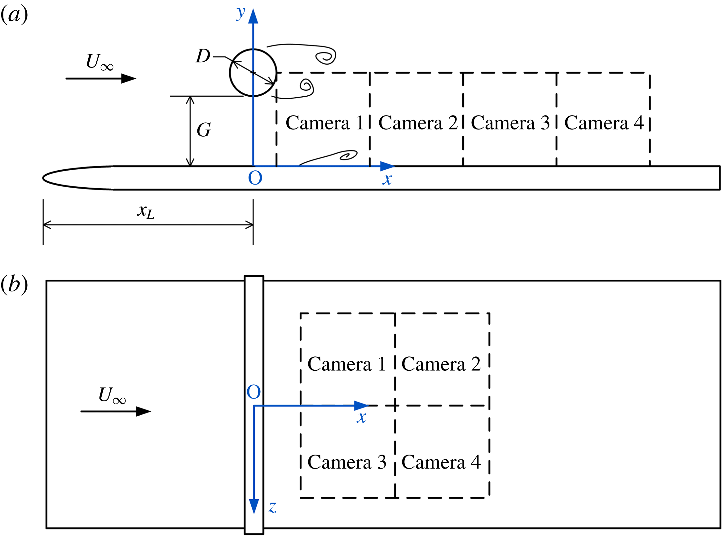
was less than 0.8 %. Figure 1 illustrates the experimental schematic and definition of the coordinates. A flat plate of dimensions 10 mm
 $\times$
500 mm
 $\times$
2500 mm (thickness
 $\times$
width
 $\times$
length) had an
 $8\,:\,1$
elliptical leading edge to prevent the flow from separation. The flat plate was horizontally positioned at the centre of the entire depth of the water tunnel. A circular cylinder with diameter
 $D=20$
mm and length
 $L=580$
mm was horizontally placed over the whole span of the flat plate, and was positioned 300 mm
 $(15D)$
downstream of the leading edge to avoid complicated receptivity problems associated with the elliptical leading edge (Schrader et al.
Reference Schrader, Brandt, Mavriplis and Henningson2010). The gap height
 $G$
between the cylinder and the flat plate was 40 mm, corresponding to a gap ratio of
 $G/D=2.0$
. This gap ratio was chosen in accordance with the flow in engineering applications, where the wake would be close enough to interact with the boundary layer underneath, but not so close that it would cause constant boundary layer separation. The Reynolds number based on the cylinder diameter,
 $Re_{D}=U_{\infty }D/{\it\nu}$
, was 1072. The flow around the circular cylinder was in the subcritical range
 $(300<Re_{D}<3\times 10^{5})$
. The flow away from the cylinder surface was laminar, with the transition occurring in the separated shear layer, and the Karman vortex street became turbulent. The shedding frequency of the circular cylinder wake vortices with the flat plate underneath was
 $f_{0}=0.75$
Hz, which was determined by looking for the dominant peak on the spectra of wall-normal velocity fluctuations in the wake. The corresponding Strouhal number
 $St=f_{0}D/U_{\infty }$
was 0.22, only slightly higher than the value
 $St=0.21$
for an isolated circular cylinder at the subcritical Reynolds number. This suggests that the effects of the wall on the shedding of wake vortices may be insignificant at the present gap ratio.
Sketch of the experimental schematic and definition of the coordinates: (a) side view; (b) plan view. The cylinder diameter in (a) is enlarged in scale for clarity.

Two-dimensional time-resolved particle image velocimetry (2DTRPIV) was used to provide quantitative information on the statistics and dynamics of the flow field. Hollow glass beads with a median diameter of
 $10~{\rm\mu}\text{m}$
and density
 $1.05~\text{g}~\text{cm}^{-3}$
were used as seeding particles. The target flow field was illuminated by a continuous laser sheet with a thickness of approximately 1 mm and a constant energy output of 8.0 W. The surface of the flat plate was painted black using flatting paint, which significantly reduced the amount of reflection. By comparing the measured unperturbed laminar boundary layer with the Blasius solution, it was found that only velocities measured below
 $y=1$
mm were affected by reflection of the wall.
Measurements were taken of the flow field in both the wall-normal plane (side view) and the streamwise–spanwise plane (plan view). In side view measurements, four charge-coupled device (CCD) cameras with a resolution of 648
 $\times$
488 pixels were aligned in the streamwise direction (see figure 1
a) in the wall-normal plane at
 $z=0$
mm. These cameras recorded particle images simultaneously under the control of a synchronizer, and yielded a combined field of view (FOV) of approximately 260 mm
 $\times$
50 mm
 $(13D\times 2.5D)$
. For plan view measurements, the four cameras were aligned differently (see figure 1
b) in a spanwise plane at
 $y=3$
mm (
 $y/D=0.15$
), and they yielded a combined FOV of approximately 140 mm
 $\times$
100 mm
 $(7D\times 5D)$
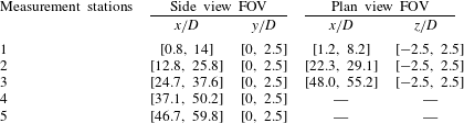
. The FOV of the four cameras was adjusted by imaging a single target at the same time, and there was an overlap of at least 5 mm between the FOV of adjacent cameras. Measurements were made at different streamwise stations, and the FOV for each measurement station is given in table 1.
Field of view (FOV) for different measurement stations.

The sampling frequency of the PIV system was 100 Hz, two orders of magnitude higher than the wake vortex shedding frequency
 $f_{0}$
of 0.75 Hz; therefore the temporal information can be regarded as time-resolved. Most of the imaged particles had diameter
 $d_{p}$
greater than two pixels, so the peak-locking effect was negligible (Christensen Reference Christensen2004). The exposure time was 3 ms. The maximum stretching of particle images in the streamwise direction was less than two pixels, so its influence on the determination of particle image displacement should be insignificant. The recorded 12-bit particle images were analysed using a multi-pass interrogation algorithm with a final interrogation window size of 16
 $\times$
8 pixels. The particle image density was 0.054 particle per pixel, so there were six to seven particle images on average in the final interrogation window. The velocity field was in the form of [
 $u(x,y,t)$
,
 $v(x,y,t)$
] for the side view and [
 $u(x,z,t)$
,
 $w(x,z,t)$
] for the plan view. This interrogation window size corresponds to a physical domain of approximately
 $1.72\times 0.86~\text{mm}^{2}$
for the side view measurement and
 $2\times 1~\text{mm}^{2}$
for the plan view measurement. There was a 50 % overlap of the interrogation windows. The spacing between adjacent velocity vectors for the side view measurement was approximately 0.43 mm in the wall-normal
 $(y)$
direction and 0.86 mm in the streamwise
 $(x)$
direction, whereas for the plan view measurement it was approximately 0.5 mm in the spanwise
 $(z)$
direction and 1.0 mm in the streamwise direction. The maximum particle displacement in the flow was more than six pixels. Using 0.1 pixel as the subpixel peak fitting uncertainty in determining the particle image displacement, the uncertainty of the velocity was estimated to be less than 2 % of the free-stream velocity. In one repetition 6350 continuous frames could be recorded, and three repetitions were taken to enlarge the sampling duration to more than 3 min.
Several previous experiments on boundary layer flow (Pan et al.
Reference Pan, Wang, Zhang and Feng2008; Wang, Pan & Zhang Reference Wang, Pan and Zhang2009; Wang, Zhang & Pan Reference Wang, Zhang and Pan2011; Zhang, Pan & Wang Reference Zhang, Pan and Wang2011; Pan, Wang & He Reference Pan, Wang and He2012; Wu, Pan & Li Reference Wu, Pan and Li2012) have been carried out using this set-up, so it could be guaranteed that a laminar boundary layer would develop along the upper surface of the flat plate when the circular cylinder was absent. The local Blasius boundary layer thickness
 ${\it\delta}_{B}$
at
 $x/D=0$
was 10.6 mm, corresponding to a
 ${\it\delta}_{B}/D$
of 0.53, so the circular cylinder in the present experiment was placed well outside the boundary layer (
 $G/{\it\delta}_{B}=3.78$
). The boundary layer Reynolds number
 $Re_{{\it\delta}^{\ast }}=U_{\infty }{\it\delta}^{\ast }/{\it\nu}$
(where
 ${\it\delta}^{\ast }$
is the displacement thickness of the Blasius boundary layer) at
 $x/D=0$
was 243, well below the critical value of 400 (White Reference White1991), the minimum Reynolds number for initial instability on the neutral stability curve. The current PIV measurements had a wall-normal resolution of
 $0.08{\it\delta}_{B}$
at
 $x/D=0$
; this resolution in terms of the boundary layer thickness would increase as the boundary layer becomes thicker downstream, especially when it undergoes transition. At
 $x/D=50$
, where the boundary layer has already become turbulent, the wall-normal resolution was approximately 2.8
 $y^{\ast }$
(where
 $y^{\ast }={\it\nu}/u_{{\it\tau}}$
is the inner length scale).
In addition to the PIV measurements, some hydrogen bubble visualizations were conducted. The hydrogen bubbles were produced from a platinum wire with a diameter of
 $25~{\rm\mu}\text{m}$
, which was welded to a holder with a span of 250 mm. Two typical working modes were used in the current study: the continuous mode, driven by a constant voltage on the wire, and the pulsed mode, driven by the periodic square-wave voltage on the wire. These two modes produced, respectively, a continuous sheet of hydrogen bubbles and so-called hydrogen bubble time lines. The flow was illuminated by a tungsten filament lamp and recorded by a Sony digital video camera at 25 f.p.s. or by CCD cameras at 50 f.p.s., depending on the size of the required FOV.
2.2 Data analysis methods
This section gives a brief overview of the methods used to analyse the PIV data, including FTLE, the Hilbert transformation and the proper orthogonal decomposition.
2.2.1 Finite-time Lyapunov exponents
Finite-time Lyapunov exponents (FTLE) can be used to find separatrices in time-dependent systems, which are often analogous to stable and unstable manifolds of time-independent systems. These separatrices are called Lagrangian coherent structures (LCS). The FTLE method offers a convenient way to reveal LCS, even for systems that have general time dependence and are defined only over a finite interval of time, which is often the case in experimental and numerical studies of fluid flow. As mentioned earlier, the ridges of the FTLE field are defined as LCS.
FTLE can be derived by considering the stretching between two neighbouring particles (Shadden et al.
Reference Shadden, Dabiri and Marsden2006). Consider an arbitrary point
 $\boldsymbol{x}$
at time
 $t_{0}$
. Let
 $\unicode[STIX]{x1D731}_{t_{0}}^{t_{0}+T}:\boldsymbol{x}(t_{0})\rightarrow \boldsymbol{x}(t_{0}+T)$
denote the flow map, which maps fluid particles from their initial location at time
 $t$
to their location at time
 $t+T$
. The FTLE are expressed as
 $$\begin{eqnarray}{\it\sigma}(\boldsymbol{x},t_{0},T)=\frac{1}{|T|}\ln \left\Vert \frac{\text{d}\unicode[STIX]{x1D731}_{t_{0}}^{t_{0}+T}(\boldsymbol{x})}{\text{d}x}\right\Vert .\end{eqnarray}$$
The quantity
 ${\it\sigma}(\boldsymbol{x},t_{0},T)$
measures the linearized maximum exponential growth rate over the interval
 $T$
of trajectories starting near point
 $\boldsymbol{x}$
at time
 $t_{0}$
;
 $T>0$
and
 $T<0$
mean forward and backward time computations, respectively. In the present work, only
 $T<0$
is used, so the ridges of high FTLE correspond to attracting LCS. The initial locations
 $\boldsymbol{x}(t_{0})$
of the virtual tracer particles are on a regular grid with a spatial resolution of 0.25 mm
 $(0.0125D)$
in both the
 $x$
and the
 $y$
directions, denser than the grid of the original PIV velocity vectors. These virtual tracer particles are then allowed to move in time following the PIV velocity. The trajectories of the particles are calculated using a fourth-order Runge–Kutta method with a time step of 0.01 s (the time interval between adjacent velocity fields). Because the velocity vectors measured with PIV are discrete data (on a grid), a cubic interpolation of the velocity data at time
 $t$
is used to obtain the local Eulerian velocity at
 $\boldsymbol{x}(t)$
. After a time interval of
 $T$
, the particles arrive at
 $\boldsymbol{x}(t_{0}+T)$
; then
 ${\it\sigma}(\boldsymbol{x},t_{0},T)$
is given in the discrete form as the logarithm of the largest singular value
 ${\it\lambda}_{max}$
of the deformation gradient matrix:
 $$\begin{eqnarray}{\it\sigma}(\boldsymbol{x},t_{0},T)=\frac{1}{|2T|}\ln \left({\it\lambda}_{max}\left\{\left[\frac{\partial \boldsymbol{x}(t_{0}+T)}{\partial \boldsymbol{x}(t_{0})}\right]^{\prime }\left[\frac{\partial \boldsymbol{x}(t_{0}+T)}{\partial \boldsymbol{x}(t_{0})}\right]\right\}\right).\end{eqnarray}$$
The ridges of
 ${\it\sigma}(\boldsymbol{x},t_{0},T)$
represent the LCS at time
 $t_{0}$
.
2.2.2 Hilbert transformation and amplitude modulation
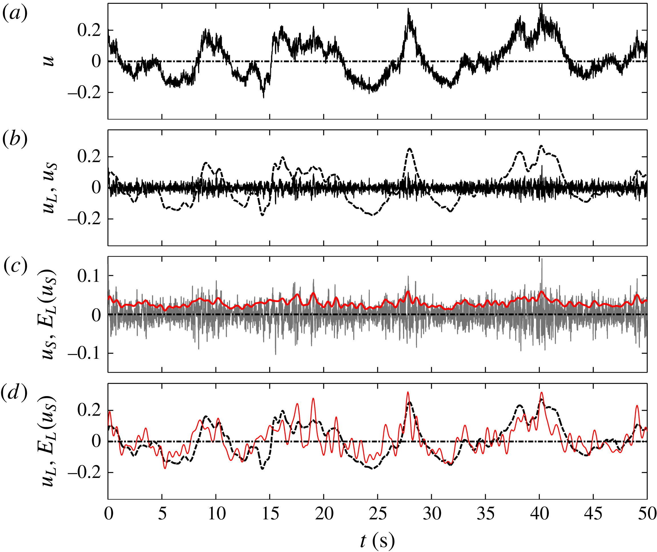
In the study of Mathis, Hutchins & Marusic (Reference Mathis, Hutchins and Marusic2009), the Hilbert transformation was applied to the spectrally filtered small-scale component of fluctuating velocity signals. They found that the small-scale structures were subject to a high degree of amplitude modulation originating from the larger scales. A detailed description of this method can be found in Mathis et al. (Reference Mathis, Hutchins and Marusic2009). Here we just give a summary of this method, dealing with the velocity traces from a single point, which does not require extra information about the advective lag needed in the two-point correlation method.
-
(1) Firstly, the fluctuating velocity
 $u(y,t)$
at a single point (
$x$
,
$y$
) (
$x$
is usually fixed) is decomposed by a cutoff frequency
$f_{c}$
into a low-frequency-band (large-scale) component
$u_{L}(y,t)$
and high-frequency-band (small-scale) component
$u_{S}(y,t)$
.
-
(2) Secondly, the Hilbert transformation is applied to the small-scale component
$u_{S}(y,t)$
to get its envelope
$E(u_{S}(y,t))$
.The Hilbert transform is useful in calculating instantaneous attributes of a time series, especially the amplitude and frequency. For a real-valued signal
$x(t)$
, its Hilbert transformation
$h(t)$
is given by (2.3)where
$$\begin{eqnarray}\displaystyle h(t)=\frac{P}{{\rm\pi}}\int _{-\infty }^{\infty }\frac{x({\it\tau})}{t-{\it\tau}}\,\text{d}{\it\tau}, & & \displaystyle\end{eqnarray}$$
$P$
is the Cauchy principal value of the integral;
$h(t)$
is a version of the original real sequence with a
$90^{\circ }$
phase shift. The associated complex analytic signal
$Z(t)$
is defined as (2.4)Here
$$\begin{eqnarray}\displaystyle Z(t)=x(t)+\text{i}h(t)=A(t)\text{e}^{\text{i}{\it\varphi}(t)}. & & \displaystyle\end{eqnarray}$$
$A(t)$
is the amplitude of
$Z(t)$
and also the envelope of
$x(t)$
; it is given by (2.5)Applying the Hilbert transformation to the small-scale fluctuation
$$\begin{eqnarray}\displaystyle A(t)=\sqrt{x^{2}(t)+h^{2}(t)}. & & \displaystyle\end{eqnarray}$$
$u_{S}(y,t)$
yields its envelope
$E(u_{S}(y_{0},t))$
, which is then low-pass filtered using the cutoff frequency
$f_{c}$
.
-
(3) Finally, the low-pass filtered envelope
$E_{L}(u_{S}(y_{0},t))$
is correlated with the large-scale component
$u_{L}(y_{0},t)$
: (2.6)where
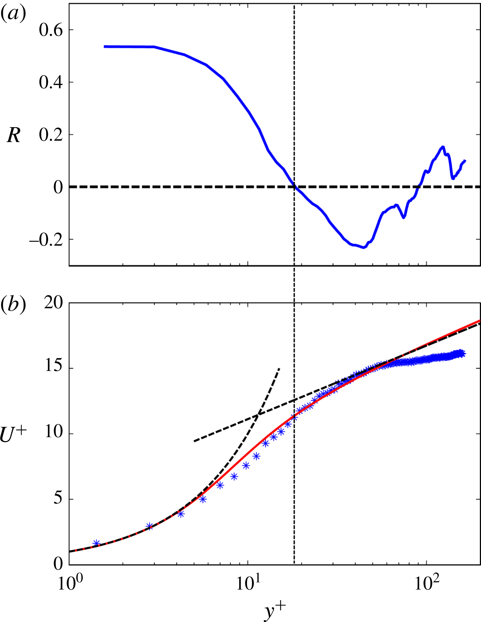
$$\begin{eqnarray}\displaystyle R(y)=\frac{\langle u_{L}(y,t),E_{L}(u_{S}(y,t))\rangle }{\Vert u_{L}(y,t)\Vert \Vert E_{L}(u_{S}(y,t))\Vert }, & & \displaystyle\end{eqnarray}$$
$\langle \cdot \rangle$
denotes the inner product and
$\Vert \cdot \Vert$
the 2-norm of a vector. The modulation effect at the selected height
$y$
can then be examined by checking the correlation coefficient
$R(y)$
.


2.2.3 Proper orthogonal decomposition
Proper orthogonal decomposition (POD) is a common tool in the analysis of fluid flow, as it is very useful in extracting the dominant flow structures from the complex flow field. In this technique, a random function is decomposed into a weighted linear sum of orthogonal eigenfunctions. The first
 $n$
eigenfunction modes of POD can capture more energy than the first
 $n$
functions of any other basis. The theory and application of the POD method are well documented in the literature (see Berkooz, Holmes & Lumley Reference Berkooz, Holmes and Lumley1993, for example), so we will not repeat the descriptions here. Since the current PIV measurement provides a large amount of instantaneous data over a large spatial extent, POD analysis of these data may be useful in extracting the dominant flow structures.
3 Experimental results
3.1 Mean velocity
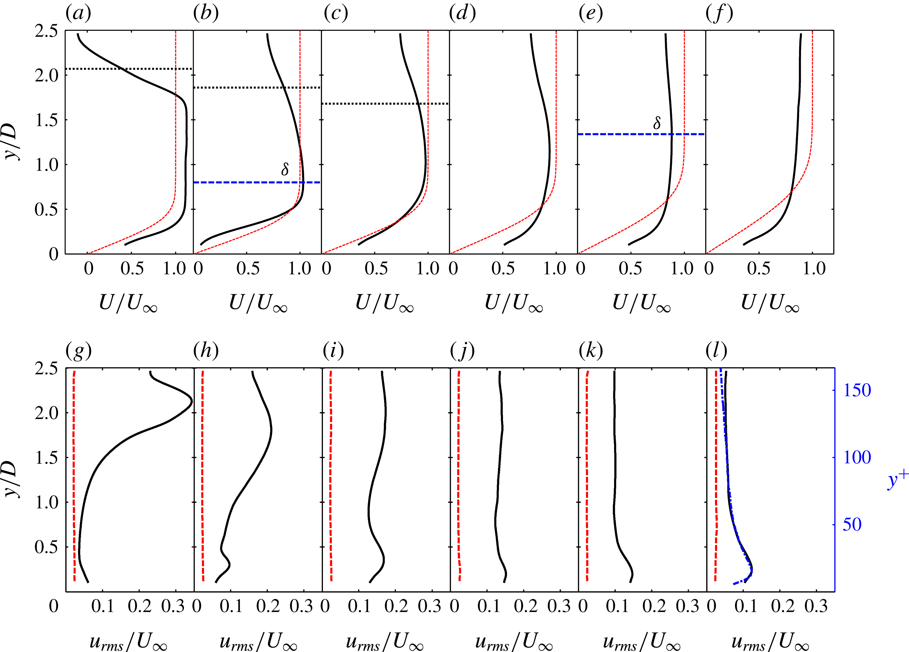
Profiles of flow velocity statistics are presented in figure 2. Figure 2(a–f) shows the mean streamwise velocity profiles at several streamwise locations. Due to the limitation of the wall-normal FOV, only the lower wake flow is captured (the circular cylinder is centred at
 $y/D=2.5$
). In the wake region, the velocity deficit behind the cylinder is evident. The half-width of an independent circular cylinder wake, defined as the distance between the centreline and the location where the velocity deficit diminishes to half of the maximum deficit, is marked for
 $x/D=2.5$
, 5 and 10. In the presence of the flat plate, these lines still provide a good estimate of the wake half-width, suggesting that the influence of the flat plate on the flow around the circular cylinder may be insignificant for
 $x/D\leqslant 10$
. The wake velocity deficit gradually decreases in the downstream locations; however, even at
 $x/D=50$
, the deficit still persists (see the profile at this location in figure 2
f). At
 $x/D=2.5$
, there is an overshoot of the mean velocity due to the acceleration of flow around the cylinder. At
 $x/D=5$
, this overshoot is still observable above
 $y/D=0.5$
. Very close to the wall, however, the mean velocity is smaller than that of the Blasius profile. This is caused by the local separation associated with the periodic formation of secondary vortices, which will be shown later. Further downstream, the profile near the wall surpasses that of the Blasius profile, indicating a boundary layer transition. As no uniform outer flow can be observed due to the existence of the wake, we adopt a definition of boundary layer thickness used in the studies of Sarkar & Sarkar (Reference Sarkar and Sarkar2009) and He et al. (Reference He, Wang and Pan2013). In this definition, the height of the maximum streamwise velocity between the wall and the wake deficit region is the boundary layer edge (as indicated by the horizontal dashed lines for the profiles at
 $x/D=5$
and
 $25$
). According to this definition, the boundary layer thickness
 ${\it\delta}$
is approximately
 $0.8D$
at
 $x/D=5$
and increases to approximately
 $1.34D$
at
 $x/D=25$
. However, further downstream at
 $x/D=50$
, where the boundary layer has already become turbulent, the mean velocity increases monotonically with wall-normal height. It has not reached a maximum or the uniform velocity, due to the limited size of the FOV. In this case,
 ${\it\delta}$
is assumed to be
 $2.5D$
to give a rough estimate of the boundary layer thickness. This corresponds to a Reynolds number of
 $Re_{{\it\tau}}=162$
(
 $Re_{{\it\tau}}={\it\delta}/y^{\ast }$
where
 $y^{\ast }={\it\nu}/u_{{\it\tau}}$
is the inner length scale of the turbulent boundary layer). The friction velocity
 $u_{{\it\tau}}$
was estimated by fitting the turbulent boundary layer profile using the Musker model (Kendall & Koochesfahani Reference Kendall and Koochesfahani2006). This estimate of
 $u_{{\it\tau}}$
has a mean error of approximately 0.5 %, so the derived results (such as
 $y^{\ast }$
) are not sensitive to this estimation.
Profiles of flow velocity statistics at several streamwise locations: (a,g)
 $x/D=2.5$
; (b,h)
 $x/D=5$
, (c,i)
 $x/D=10$
, (d,j)
 $x/D=15$
, (e,k)
 $x/D=25$
, (f,l)
 $x/D=50$
. (a–f) Mean streamwise velocity profiles (black solid lines) and local Blasius profiles (red dashed lines); the blue horizontal dashed lines at
 $x/D=5$
and
 $25$
indicate the local boundary layer edges, and the black horizontal dotted lines indicate the half-width of the wake of an isolated circular cylinder (note that the cylinder is centred at
 $y/D=2.5$
). (g–l) Root mean square of streamwise velocity fluctuations,
 $u_{rms}$
, where black solid lines and red dashed lines represent
 $u_{rms}$
profiles for the flow with and without the presence of the cylinder, respectively, and the blue dash–dot line at
 $x/D=50$
represents the canonical turbulent boundary layer triggered by a trip wire at
 $Re_{{\it\tau}}=173$
(Pan, Wang & Zhang Reference Pan, Wang and Zhang2009); inner-scaled coordinates are given for
 $x/D=50$
.

Profiles of the streamwise fluctuation intensity,
 $u_{rms}$
, are shown in figure 2(g–l), from which it can be seen that the presence of the cylinder greatly disturbs the flow over the flat plate. In the wake, a dominant peak appears in the profile, due to magnification of disturbances in the lower shear layer and the subsequent formation of low wake vortices. This peak decreases with increase of streamwise location, corresponding to weakening of the wake vortices as they convect downstream. On the other hand, in the near-wall region, a peak becomes more and more evident. At
 $x/D=10$
the peak value even surpasses the disturbance level in the wake, which is a more direct indication of the boundary layer transition. At
 $x/D=50$
, the
 $u_{rms}$
profile compares well with a canonical turbulent boundary layer (the blue dash–dot line, which was rescaled by setting its peak value to the same value as
 $12.3\,\%\times U_{\infty }$
in the present study), although there is a small discrepancy for
 $y/D>2$
due to the influence of the cylinder wake. This suggests that the boundary layer has already become turbulent at this location.
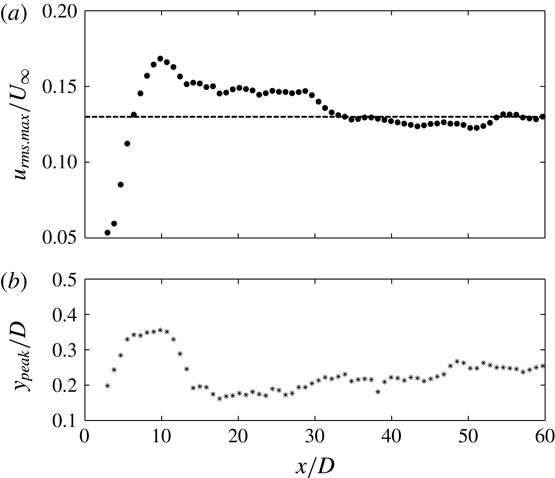
Evolution of maximum disturbance and its wall-normal position in the boundary layer: (a) streamwise growth of the maximum of fluctuation intensity,
 $u_{rms.max}$
, in the boundary layer, with the black dashed line indicating
 $u_{rms.max}/U_{\infty }$
in a canonical turbulent boundary layer at approximately
 $Re=300$
(Spalart Reference Spalart1988); (b) wall-normal position of
 $u_{rms.max}$
in the boundary layer.

To show more clearly the growth of the disturbance in the boundary layer, the maximum fluctuation intensity
 $u_{rms.max}$
in the near-wall region in the profiles of figure 2(g–l) is plotted against streamwise location in figure 3(a). It is evident that the disturbance level in the boundary layer experiences a rapid growth immediately downstream of the cylinder. After reaching a peak value at approximately
 $x/D=$
10, the disturbance level slowly decreases and finally reaches a nearly constant level after
 $x/D>35$
, close to the value of the canonical turbulent boundary layer (Spalart Reference Spalart1988). The fast growth of the disturbance in the boundary layer has also been reported in the experimental study of Mandal & Dey (Reference Mandal and Dey2011) and in the simulation study of Ovchinnikov et al. (Reference Ovchinnikov, Piomelli and Choudhari2006). As will be shown later, this fast growth is closely related to the formation and evolution of secondary vortices in the boundary layer. In figure 3(b), the streamwise variation of the position
 $y_{peak}$
, which is the wall-normal height of
 $u_{rms.max}$
, is presented. Interestingly, immediately behind the cylinder,
 $y_{peak}$
increases rapidly, in accordance with the fast disturbance growth. After reaching a maximum of approximately
 $y_{peak}/D=0.35$
around
 $x/D=10$
, the
 $y_{peak}$
drops to a much lower wall-normal height. The increase of
 $y_{peak}$
may be related to the local separation and lift-up of the shear layer in the near-wall region (discussed further below). The movement of
 $u_{rms.max}$
towards the wall in the transition process is in agreement with other wake-induced transition studies (Ovchinnikov et al.
Reference Ovchinnikov, Piomelli and Choudhari2006; Pan et al.
Reference Pan, Wang, Zhang and Feng2008; Mandal & Dey Reference Mandal and Dey2011). Further downstream,
 $y_{peak}$
experiences a slow increase and reaches approximately
 $y_{peak}/D=0.25$
at
 $x/D=50$
, which corresponds to an inner-scale normalized wall-normal height of
 $y^{+}=16$
. This is close to the value of
 $y^{+}=15$
for a turbulent boundary layer, confirming that the boundary layer has reached a turbulent state at this location. For the benefit of the following discussion, we divide the boundary layer flow downstream of the cylinder roughly into three stages: the beginning of transition (the fast-growing stage of the disturbance,
 $x/D<10$
), the middle stage of transition (the slow decay stage,
 $10<x/D<35$
) and the turbulent state (the nearly constant stage,
 $x/D>35$
).
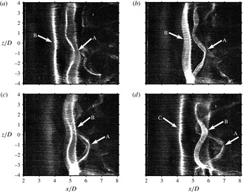
Hydrogen bubble visualization of spanwise secondary vortices at the beginning of transition: plan view. The platinum wire was working in continuous mode and was placed parallel to the flat plate at
 $x/D=2$
and a wall-normal height of
 $y_{w}/D=0.1$
. Panels (a–d) are a time sequence with a time interval of
 ${\rm\Delta}t/T_{0}=0.225$
(where
 $T_{0}$
is the shedding period of the wake vortices) between two consecutive instants; the arrows A, B and C indicate the vortex tubes. See supplementary movie 1 available at http://dx.doi.org/10.1017/jfm.2016.81.

3.2 Flow structures
3.2.1 LCS revealed by hydrogen bubble visualizations
The flow structures in the boundary layer immediately downstream of the cylinder are revealed by the hydrogen bubble visualization shown in figure 4. Spanwise secondary vortices are periodically induced in the near-wall region by the passing wake vortices. The spanwise vortex tubes of the secondary vortices (indicated by arrows A, B and C) are visualized by the high-concentration regions of hydrogen bubbles. The vortex tube is nearly two-dimensional at first, and loses its spanwise coherence through three-dimensional destabilization as it convects downstream. In this three-dimensional destabilization process,
 ${\it\Lambda}$
vortices are formed. Similar spanwise instability developing on a two-dimensional vortex tube can often be observed in a free shear layer (Pierrehumbertt & Widnall Reference Pierrehumbertt and Widnall1982; Ashurst Reference Ashurst1988; Lasheras & Choi Reference Lasheras and Choi1988). The
 ${\it\Lambda}$
vortex is tilted in the streamwise direction (not shown in the plan view visualization here). Its head is located higher in the wall-normal direction and moves faster than its legs (see Pan et al.
Reference Pan, Wang, Zhang and Feng2008). It has been pointed out in an earlier study of He & Wang (Reference He and Wang2015) that the three-dimensional destabilization is triggered by the spanwise instability of wake vortices. As
 ${\it\Lambda}$
vortices are stretched in the streamwise direction, their counter-rotating streamwise-stretched legs would induce a streamwise elongated low-speed region in the boundary layer, so low-frequency disturbances associated with them will gradually become dominant in the growth of disturbances in the boundary layer (He et al.
Reference He, Wang and Pan2013). Corresponding to the formation and destabilization of the secondary vortices, the total disturbance experiences a fast growth, as shown in figure 3(a).
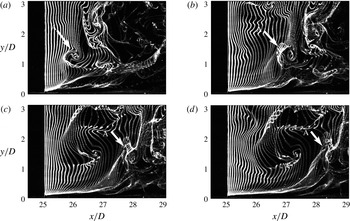
Hydrogen bubble time line visualization of a hairpin vortex in the middle stage of transition: side view. The platinum wire was working in pulsed mode with a frequency of 16 Hz and was placed perpendicular to the flat plate at approximately
 $x/D=25$
. Panels (a–d) are a time sequence with an interval of
 $U_{\infty }{\rm\Delta}t/{\it\delta}=0.75$
(where
 ${\it\delta}/U_{\infty }$
is the boundary layer turnover time) between two consecutive time instants. See supplementary movie 2.

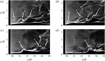
Hydrogen bubble time line visualization of a hairpin vortex packet in the turbulent boundary layer: side view. The platinum wire was working in pulsed mode with a frequency of 16 Hz and was placed perpendicular to the flat plate at approximately
 $x/D=50$
. Panels (a–d) are a time sequence with an interval of
 $U_{\infty }{\rm\Delta}t/{\it\delta}=0.80$
(where
 ${\it\delta}/U_{\infty }$
is the boundary layer turnover time) between two consecutive time instants. See supplementary movie 3.

According to Pan et al. (Reference Pan, Wang, Zhang and Feng2008), the
 ${\it\Lambda}$
vortices would evolve into primary hairpin vortices downstream. Figure 5 shows such a primary hairpin vortex (with its head indicated by arrow A) in the middle stage of boundary layer transition. Unlike figure 4, the hydrogen bubble visualization here was in a wall-normal plane and the platinum wire was working in pulsed mode. The hairpin vortex in figure 5 is the result of further lift-up of the
 ${\it\Lambda}$
vortex head and streamwise stretching of the
 ${\it\Lambda}$
vortex legs. At
 $x/D=25$
, the estimated boundary layer thickness
 ${\it\delta}/D$
is 1.34. So the scale of the primary hairpin vortex spans the boundary layer in the wall-normal direction, with its legs close to the wall and its head extending out of the boundary layer (see figure 5
d). This means that it is a large and strong primary hairpin vortex which, according to Zhou et al. (Reference Zhou, Adrian, Balachandar and Kendall1999), could generate new hairpin vortices and lead to the formation of a hairpin packet in the boundary layer.
The hydrogen bubble visualization in figure 6 shows the hairpin packet in the turbulent boundary layer. It can be seen that hairpin B is generated by hairpin A, judging by their spatial positions and the continuity of the bright concentrated hydrogen bubble line. The mechanism behind the generation of a new hairpin vortex has been addressed by Smith et al. (Reference Smith, Walker, Haidari and Sobrun1991) and Zhou et al. (Reference Zhou, Adrian, Balachandar and Kendall1999). It has been explained that for a primary hairpin vortex above a certain strength threshold, a kink forms in the long legs of the primary hairpin vortex, owing to their mutual induction. The shear layer lifted up between the legs rolls up into a spanwise vortex near the kink, while the long legs of the primary vortex sever at this point. The upstream segments of the legs then connect with the spanwise vortex to form a new hairpin vortex. This regeneration process could go on to produce a chain of hairpin vortices in the streamwise direction, forming a so-called hairpin packet. The current visualization is a cross-section cutting through the head and between the legs of the hairpin vortices, so only the hairpin heads and the shear layer between the legs can be seen. The visualization here reveals a regeneration process consistent with the above description, although some aspects are missing due to the limitation of planar observation. Similarly, hairpin D is generated by hairpin C. The streamwise alignment of these four hairpin vortices can be viewed as a hairpin packet (or perhaps two hairpin packets each containing two hairpins, depending on the relationship between vortex B and vortex C). It should be noted here that a very long low-speed streak is expected to be generated under this packet, which can be inferred from the lack of hydrogen bubbles beneath the hairpin vortices due to the upward induction of the counter-rotating hairpin legs. Evidence in support of this will be given later.
3.2.2 LCS revealed by FTLE
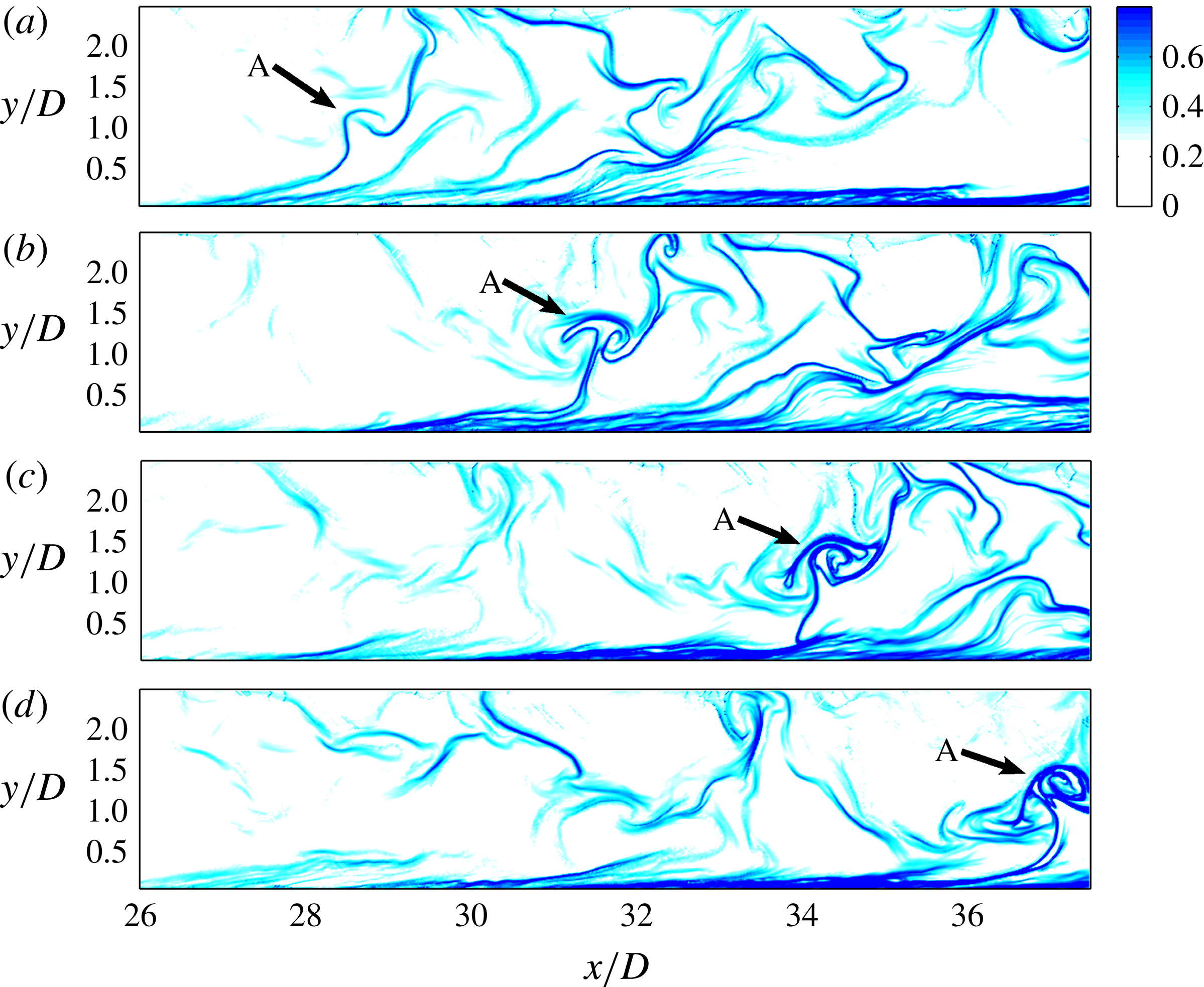
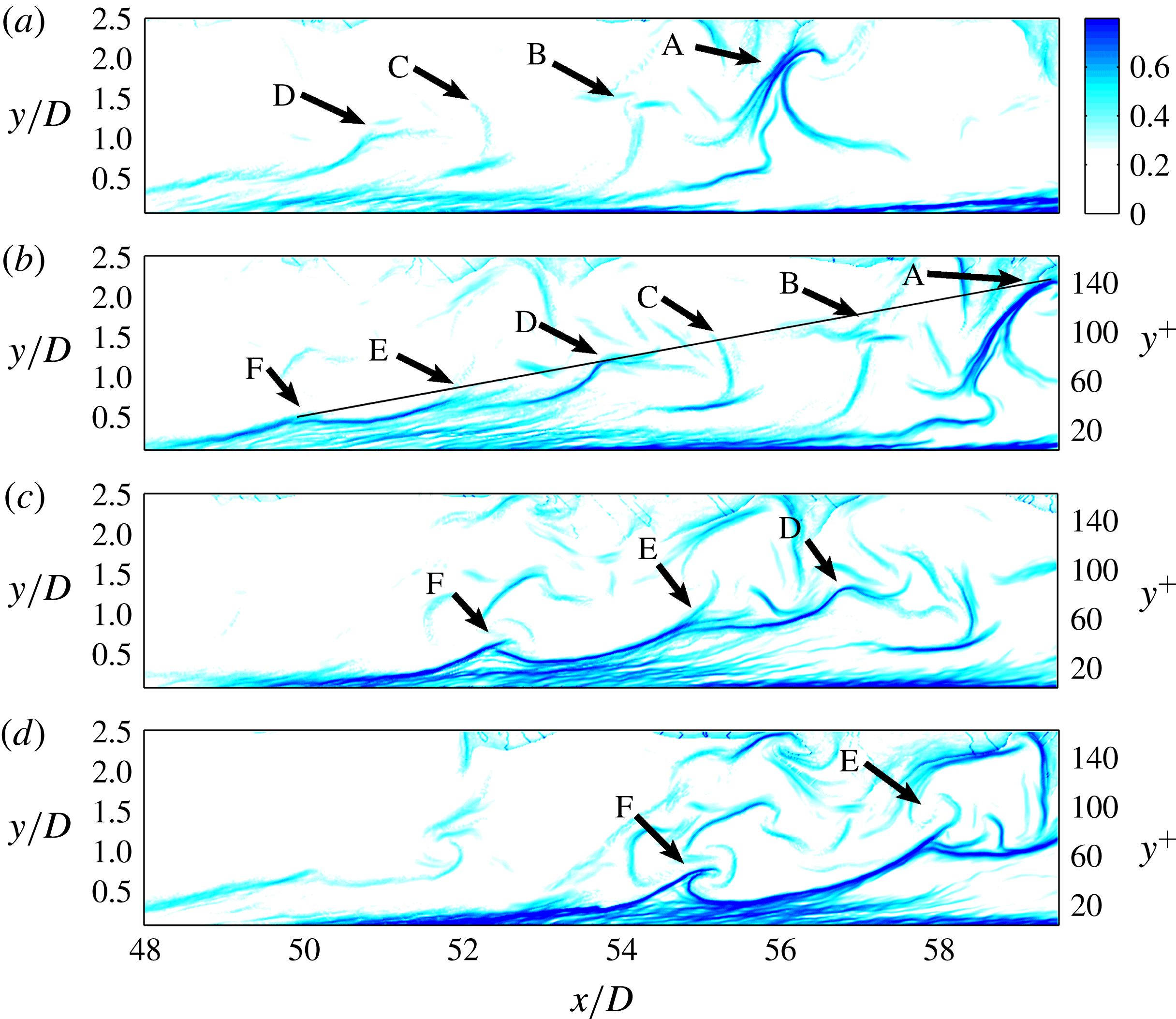
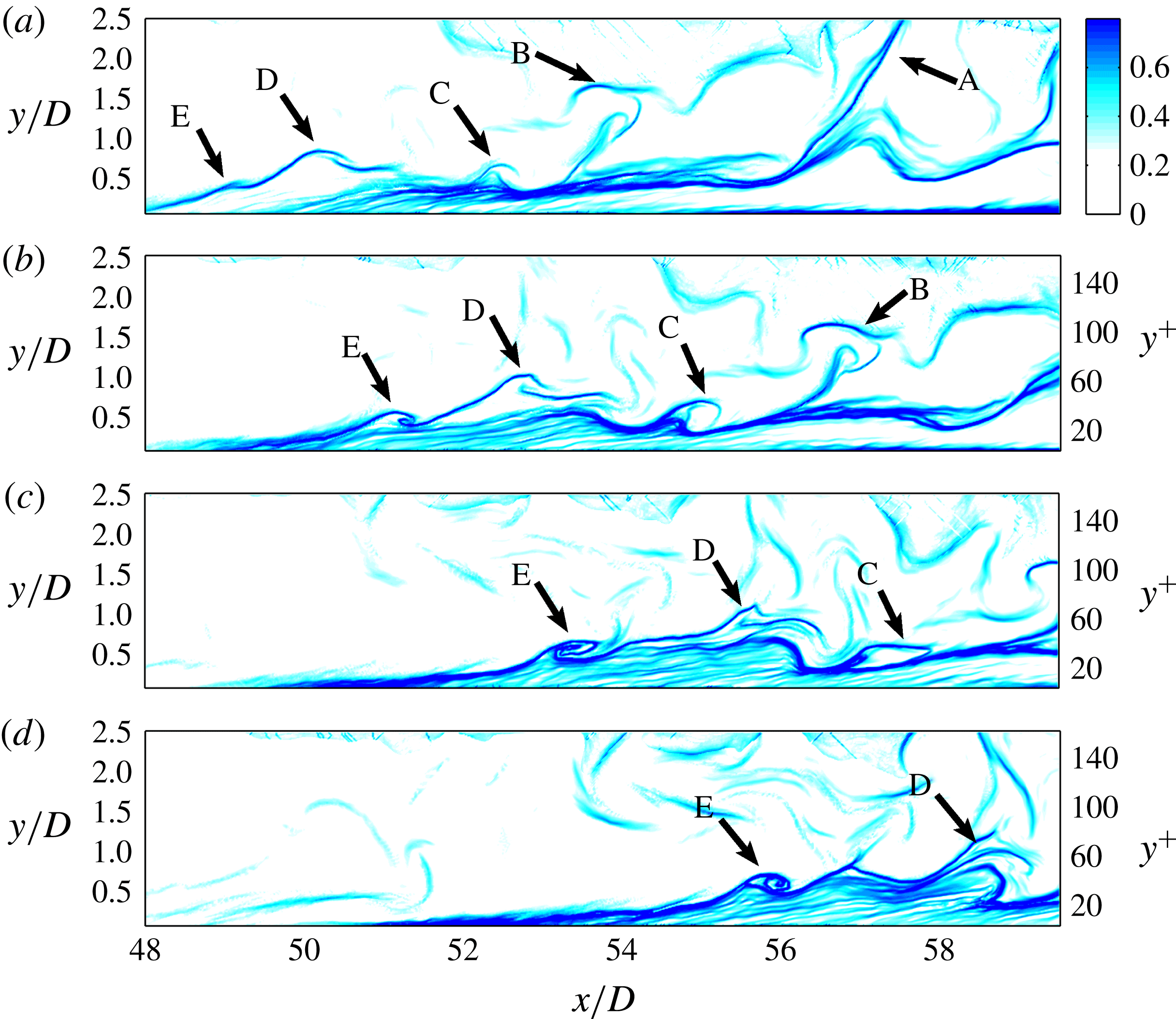
The evolution of LCS, from the beginning of transition until the formation of the turbulent boundary layer, has also been revealed by the FTLE fields shown in figures 7–10.
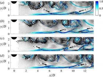
Secondary vortices induced by the wake vortices at the beginning of transition. Panels (a–d) are a time sequence with an interval of
 ${\rm\Delta}t/T_{0}=0.56$
(where
 $T_{0}$
is the shedding period of the wake vortices) between two consecutive time instants. The LCS are revealed by the FTLE field with an integration time of
 $T/T_{0}=-3$
(negative time means backward integration). The vectors show the fluctuation velocity. See supplementary movie 4.

A hairpin vortex in the middle stage of boundary layer transition. Panels (a–d) are a time sequence with an interval of
 $U_{\infty }{\rm\Delta}t/{\it\delta}=2.5$
between two consecutive time instants. The LCS are revealed by the FTLE field with an integration time of
 $U_{\infty }T/{\it\delta}=-10.0$
(backward integration). See supplementary movie 5.

A hairpin packet in the turbulent boundary layer. Panels (a–d) are a time sequence with an interval of
 $U_{\infty }{\rm\Delta}t/{\it\delta}=1.34$
between two consecutive time instants. The LCS are revealed by the FTLE field with an integration time of
 $U_{\infty }T/{\it\delta}=-5.36$
(backward integration). See supplementary movie 6.

Another example of hairpin packets in the turbulent boundary layer. Panels (a–d) are a time sequence with an interval of
 $U_{\infty }{\rm\Delta}t/{\it\delta}=1.34$
between two consecutive time instants. The LCS are revealed by the FTLE field with a normalized integration time of
 $U_{\infty }T/{\it\delta}=-5.36$
(backward integration). See supplementary movie 7.

Figure 7 shows the FTLE fields immediately downstream of the cylinder, which are computed from the PIV data with an integration time length of 4 s (or three wake vortex shedding periods). A longer integration time would not show greater detail of the LCS, because most of the virtual tracers have already convected out of the domain. Backward integration is used in this investigation, so attracting Lagrangian coherent structures are revealed. The fluctuating Eulerian velocities are shown by the vectors. It can be seen that the coherent structures are captured very well by this FTLE method. In the wake region behind the cylinder (
 $y/D>1$
), the captured structures are the lower shear layer and the wake vortices shed from the cylinder. In the near-wall region, the formation of secondary vortices under the induction of the wake vortices can be seen very clearly. Take, for example, vortex B in figure 7(a); under the induction of the lower wake vortex shed from the circular cylinder, there is a local separation in the boundary layer, resulting in a lifted shear layer. Due to the continuous induction of the wake and the instability of the shear layer, the shear layer rolls into a vortex. The secondary vortices have the same periodicity as the wake vortices. The FTLE results further confirm the existence of secondary vortices induced by the wake vortices. Note that after
 $x/D>6$
, the vortices indicated by the arrows are just one cross-section of the spanwise deformed secondary vortices (
 ${\it\Lambda}$
vortices shown in figure 4).
Figure 8 shows a single hairpin vortex (indicated by arrow A) in the middle stage of boundary layer transition for
 $x/D>26$
. The hairpin vortex here and the one shown in the hydrogen bubble visualization in figure 5 are very much alike. It is also similar to the isolated hairpin vortex shown by Green et al. (Reference Green, Rowley and Haller2007) using the FTLE method. The size of the vortex suggests that it may be able to generate a hairpin packet as it convects downstream. Although its subsequent evolution cannot be directly followed due to limitation of the FOV, a growing population of hairpin packets can be seen in the boundary layer downstream.
A hairpin packet is shown in figure 9 for
 $x/D>48$
. The boundary layer has become turbulent at this streamwise location. The inner-scaled wall-normal coordinate
 $y^{+}$
is given on the right of the plots. This hairpin packet seems to consist of six hairpin vortices (indicated by the arrows A–F), with the largest primary hairpin vortex (arrow A) at the downstream end and the youngest one at the upstream end (arrow F). Hairpin vortices B and C are not as clear as the rest of the vortices. This may be attributed to the fact that in a turbulent boundary layer, instead of being perfectly symmetrical about the middle plane, hairpin vortices are usually asymmetric one-sided cane-like structures (Zhou et al.
Reference Zhou, Adrian, Balachandar and Kendall1999). As a result, the hairpin vortices in a packet will not align perfectly along the streamwise direction, but rather will stagger to some extent in the spanwise direction. The process of generation of new hairpin vortices (such as hairpin vortices E and F) is also very similar to that described in the study of Green et al. (Reference Green, Rowley and Haller2007), who used the FTLE method to detect the simulated evolution of an isolated hairpin vortex.
The packet shown in figure 9 is consistent with the coherent packets in the turbulent boundary layer shown by Adrian and coworkers (Zhou et al.
Reference Zhou, Adrian, Balachandar and Kendall1999; Adrian, Meinhart & Tomkins Reference Adrian, Meinhart and Tomkins2000b
; Adrian Reference Adrian2007). A line connecting the hairpin vortex heads yields a slope of approximately
 $11^{\circ }$
, which is very close to the mean angle of
 $12^{\circ }$
reported by Adrian et al. (Reference Adrian, Meinhart and Tomkins2000b
). However, this angle only gives the characteristic slope of the envelope of hairpin packets. If we look more locally, the inclination angle for a single hairpin vortex (see hairpin vortex A in figure 9, for example) is much larger than the slope of the envelope. (The local inclination angle of LCS will be given later.) The average streamwise distance between the hairpin vortex heads in figure 9(b) is approximately
 $l/D=2$
, corresponding to
 $l^{+}=130$
(where
 $l^{+}=l/y^{\ast }$
), again in agreement with the average spacing of 100–150 in the experimental measurements of Adrian et al. (Reference Adrian, Meinhart and Tomkins2000b
). The total streamwise extent of this hairpin packet is approximately 700 wall units. It should be emphasized again that due to the induction of the legs of hairpins in the packet, a very long low-speed region can be expected near the wall under the packet. It should also be mentioned that hairpin packets can be observed in the middle stage of transition occasionally, but with very low chance and a smaller streamwise length scale.
Figure 10 gives another example of hairpin packets in the turbulent boundary layer. Two smaller packets are observed here, but they seem to form an even larger structure than the packet in figure 9. One packet consists of hairpin vortices A, B and C, while the other consists of D and E. The structure indicated by arrow A may be a primary hairpin vortex with its head extending out of view. The streamwise alignment of these two packets forms an even larger structure with streamwise length comparable to the streamwise FOV. This observation conforms to the model proposed by Kim & Adrian (Reference Kim and Adrian1999), which describes the creation of very large-scale motions (VLSM) in the turbulent boundary layer through the coherent alignment of hairpin packets in the streamwise direction. However, it should be clarified here that the Reynolds number in the present study is very low (just above
 $Re_{{\it\tau}}=160$
), so there is no clear separation of scales between the near-wall structures and the VLSM typically seen in the outer layer. The very large structure observed in figure 10 consists of only two hairpin packets.
Although this structure has a roughly estimated streamwise extent close to 5
 ${\it\delta}$
(it is assumed that
 ${\it\delta}=2.5D$
at
 $x/D=50$
), its inner-scaled streamwise length is approximately 800 wall units, close to the streamwise length of low-speed streaks in the viscous sublayer in a turbulent boundary layer (approximately 1000 wall units). Therefore it may not be a well-defined VLSM. Nevertheless, the hierarchy of scales in the present study, including the hairpin vortices, the hairpin packets and the observed even-larger structures, suggests that the same mechanism for creating VLSM may exist at lower Reynolds numbers, at least for the current wake-induced boundary layer transition scenario. For convenience, we still refer to the largest structure observed in figure 10 as VLSM in the present study.
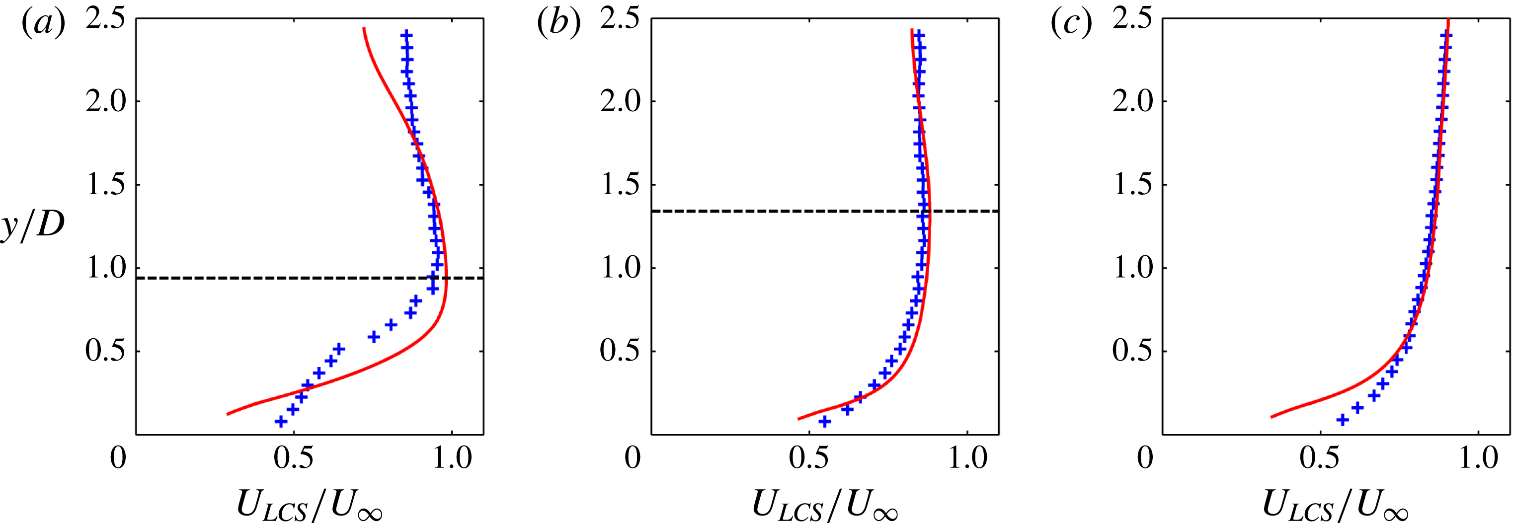
Mean streamwise convection velocity of LCS at (a)
 $x/D=7.5$
, (b)
 $x/D=25$
and (c)
 $x/D=50$
. The plus symbols represent the mean convection velocity of LCS and the red solid lines are the mean streamwise Eulerian velocity profiles. The black horizontal dashed lines in (a) and (b) indicate the local boundary layer thickness.

The above results reveal the evolution of LCS in the boundary layer. First, spanwise secondary vortices are periodically induced by the wake vortices shed from the circular cylinder. Their three-dimensional destabilization leads to the formation of
 ${\it\Lambda}$
vortices, which further evolve into primary hairpin vortices in the transitional boundary layer. The primary hairpin vortex can generate new hairpin vortices upstream, resulting in the formation of a coherent hairpin packet. The regeneration process of hairpin vortices increases their population, and the boundary layer is eventually populated with hairpin packets and becomes turbulent. This evolution scenario has previously been visualized by Pan et al. (Reference Pan, Wang, Zhang and Feng2008).
The above hydrogen bubble visualizations and FTLE fields reveal qualitatively similar evolution of the LCS. However, the FTLE method has some advantages. First, it does not rely on physical tracers to reveal the flow structures. Physical tracers such as hydrogen bubbles will dissipate into the water after a while, putting a limit on the size of the visualized area. Moreover, the capability of the hydrogen bubbles to follow the flow decreases with increase of the flow velocity. Secondly, the FTLE fields are derived from PIV data, so quantitative statistics can be extracted from them. The statistics of the LCS, including their mean convection velocity and average inclination angle, are presented in the following subsections.
3.2.3 Mean convection velocity and average inclination angle of LCS
The wall-normal profiles of the mean streamwise convection velocity at three different streamwise locations are displayed in figure 11. The mean convection velocity is calculated based on two-point cross-correlation. For given points B and C with a streamwise displacement of
 ${\rm\Delta}x$
between them, the mean streamwise convection velocity at the middle point A is given by
 $U_{LCS}={\rm\Delta}x/{\rm\Delta}t_{BC}$
, where
 ${\rm\Delta}t_{BC}$
is the time for the LCS to travel from the upstream point B to the downstream point C. The value of
 ${\rm\Delta}t_{BC}$
can be determined from the cross-correlation coefficients
 $R(x_{A},y_{A},{\it\tau})$
of the time sequences of FTLE at B and C,
 $$\begin{eqnarray}\displaystyle R(x_{A},y_{A},{\it\tau})=\frac{\langle {\it\sigma}(x_{B},y_{B},t),{\it\sigma}(x_{C},y_{C},t+{\it\tau})\rangle }{\Vert {\it\sigma}(x_{B},y_{B},t)\Vert \Vert {\it\sigma}(x_{C},y_{C},t+{\it\tau})\Vert }, & & \displaystyle\end{eqnarray}$$
where
 $\langle \cdot \rangle$
denotes the inner product and
 $\Vert \cdot \Vert$
the 2-norm of a vector. The time
 ${\rm\Delta}t_{BC}$
corresponds to the peak of the correlation coefficient
 $R(x_{A},y_{A},{\rm\Delta}t_{BC})$
. In the present study,
 ${\rm\Delta}x$
is chosen to be 10 mm
 $(0.5D)$
. This is a small distance considering that the streamwise variation of mean velocity is slow, but it is large enough to yield an accurate result (as
 ${\rm\Delta}t_{BC}$
is the denominator in determining
 $U_{LCS}$
, a value of
 ${\rm\Delta}t_{BC}$
that is too small would result in large uncertainty). The uncertainty in determining the mean convection velocity is estimated to be less than 2 % of
 $U_{\infty }$
.
Figure 11(a) gives the wall-normal profile of
 $U_{LCS}$
, the mean streamwise convection velocity of LCS, at
 $x/D=7.5$
. The black horizontal dashed line indicates the local boundary layer thickness; here
 $U_{LCS}$
is compared with the local mean streamwise Eulerian velocity
 $U$
(the red solid line), and they do not exhibit any agreement across the measured wall-normal range. In the wake region, where there is a velocity deficit due to the separation behind the circular cylinder,
 $U_{LCS}$
is distinctly larger than
 $U$
. In the outer part of the boundary layer, the mean Eulerian velocity
 $U$
is higher than
 $U_{LCS}$
. It should be noted here that very close to the wall,
 $U_{LCS}$
becomes larger again. Generally speaking,
 $U_{LCS}$
exhibits a smaller wall-normal gradient than
 $U$
. This suggests that the LCS can resist the strong shearing effect of the mean flow to some extent, in accordance with the observed tendency of LCS to maintain their general shapes in the flow for a long time. In the middle stage of transition at
 $x/D=25$
(figure 11
b), the differences between
 $U_{LCS}$
and
 $U$
become insignificant but are still observable, especially in the region very close to the wall. For the turbulent boundary layer (at
 $x/D=50$
, figure 11
c),
 $U_{LCS}$
agrees well with
 $U$
except in the near-wall region (below
 $y^{+}=30$
). Adrian et al. (Reference Adrian, Meinhart and Tomkins2000b
) have already reported that the mean streamwise convection velocity of the hairpin vortex heads is in agreement with the mean flow velocity in the turbulent boundary layer. This implies that in the outer part of a turbulent boundary layer, the streamwise flow transport is determined by the convection of LCS. In the inner layer, however, due to the non-slip boundary condition and the dominant role of viscosity,
 $U$
is much smaller than
 $U_{LCS}$
. This difference near the wall between the mean convection velocity and the Eulerian velocity has been reported by Del Alamo & Jimenez (Reference Del Alamo and Jimenez2009), Pan et al. (Reference Pan, Wang and Zhang2009) and Renard & Deck (Reference Renard and Deck2015).
Aside from the mean convection velocity, the average inclination angle
 ${\it\gamma}$
of the LCS has also been extracted from the FTLE fields. The computation of
 ${\it\gamma}$
is based on autocorrelation of the FTLE fields. The autocorrelation coefficients
 $R(x_{0},y_{0},{\rm\Delta}x,{\rm\Delta}y)$
are given by
 $$\begin{eqnarray}\displaystyle R(x_{0},y_{0},{\rm\Delta}x,{\rm\Delta}y)=\frac{\langle {\it\sigma}(x_{0},y_{0},t),{\it\sigma}(x_{0}+{\rm\Delta}x,y_{0}+{\rm\Delta}y,t)\rangle }{\Vert {\it\sigma}(x_{0},y_{0},t)\Vert \Vert {\it\sigma}(x_{0}+{\rm\Delta}x,y_{0}+{\rm\Delta}y,t)\Vert }, & & \displaystyle\end{eqnarray}$$
where
 $(x_{0},y_{0})$
is the autocorrelation base point and
 ${\rm\Delta}x$
and
 ${\rm\Delta}y$
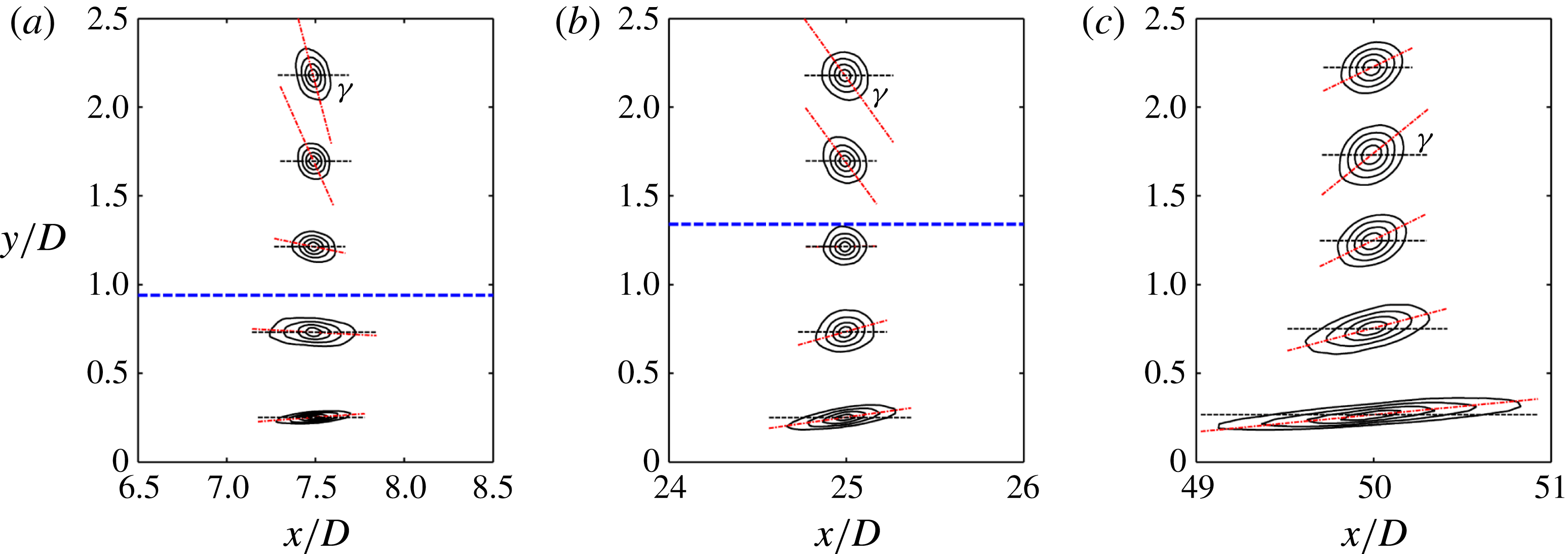
are the streamwise and wall-normal displacements, respectively. Figure 12 shows the contours of autocorrelation coefficients at some typical locations. The contours appear to be elliptical in shape. The average inclination angle
 ${\it\gamma}$
of the LCS at a certain point is defined as the acute angle made by the major axis of the elliptical contours (red dash–dot lines) with the horizontal direction (horizontal black dashed lines);
 ${\it\gamma}$
will be positive if the major axis is rotated in the counterclockwise direction. This definition, depending on the major axis, is in accordance with the narrow shape of ridge lines in the FTLE field. The contours at
 $x/D=7.5$
in figure 12(a) show that the boundary layer region has small but positive
 ${\it\gamma}$
, while large negative
 ${\it\gamma}$
can be observed in the wake region. This agrees with the result shown in figure 7, where a nearly horizontal shear layer can be found close to the wall, while the shear layer shed from the lower side of the circular cylinder mostly exhibits negative angles at this streamwise location. The negative
 ${\it\gamma}$
in the wake is still present at the middle stage of transition (at
 $x/D=25$
, figure 12
b), while the inclination angle in the boundary layer seems to be larger than that at
 $x/D=7.5$
. At
 $x/D=50$
(figure 12
c), where the boundary layer has become turbulent and the influence of the wake can be regarded as insignificant,
 ${\it\gamma}$
is positive at all wall-normal heights. It should be noticed that the streamwise extent of the correlation contours close to the wall shows a continual increase. This is consistent with the visualizations in §§ 3.2.1 and 3.2.2, including the streamwise stretching of the secondary vortices during the three-dimensional destabilization (see figure 4) and the formation of hairpin packets (see figures 9 and 10).
Contours of the correlation coefficients of the FTLE field at selected wall-normal locations
 $y/D=0.25$
, 0.75, 1.25, 1.75 and 2.25: (a) at
 $x/D=7.5$
; (b) at
 $x/D=25$
; (c) at
 $x/D=50$
. The lowest contour level is 0.6 and the increment between two adjacent contour levels is 0.1. The red dash–dot lines indicate the directions of the major axes of the elliptical fitting of the contours (defined in the text); the black thin dashed lines indicate the horizontal direction;
 ${\it\gamma}$
is the average inclination angle of LCS. The blue thick dashed lines in (a) and (b) indicate the local boundary layer thickness.

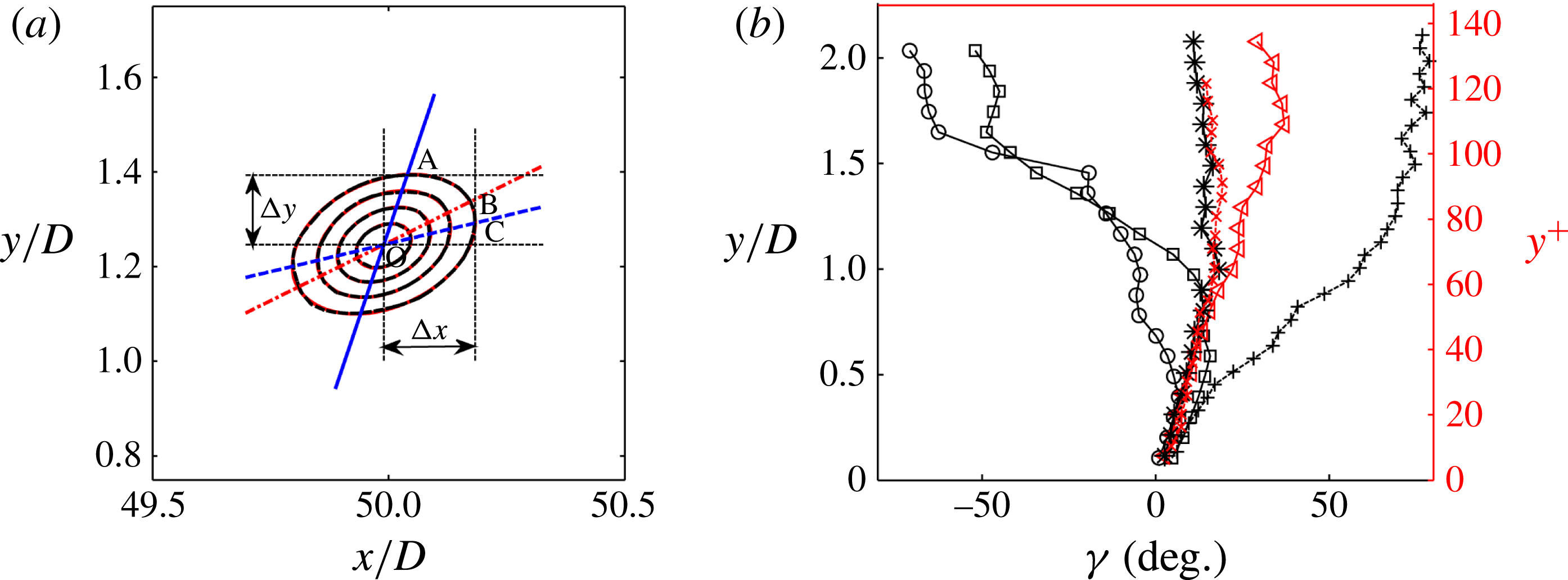
Figure 13(a) gives an example of determining the major axis of correlation contours. Each contour at the levels 0.6, 0.7, 0.8 and 0.9 is fitted with an ellipse. All the fitted ellipses nearly overlay the contours in figure 13(a). Because the angles of the major axes vary for different levels, an average is taken among the levels 0.7, 0.8 and 0.9. The variation of angles among these three levels increases with the wall-normal height. The relative uncertainty in determining the average angle here is approximately 6 %. This means an absolute uncertainty of less than
 $1^{\circ }$
below
 $y/D<0.5$
. The averaged direction of the major axis is indicated by line OB in figure 13(a).
(a) An example of elliptical fitting of the correlation contours. The centre of the contour is point O at
 $x/D=50$
and
 $y/D=1.25$
(
 $y^{+}=81$
). The lowest contour level is 0.6 and the increment between two adjacent contour levels is 0.1. The contour of the correlation coefficients (black dashed line) and the elliptical fitting at each level (red solid line) nearly overlay each other. The red dash–dot line indicates the average direction of the major axes. The blue solid line OA represents the angle obtained by two-point correlation with a fixed
 ${\rm\Delta}y$
. The blue dashed line OC represents the angle obtained by two-point correlation with a fixed
 ${\rm\Delta}x$
. (b) Inclination angle of LCS at several streamwise locations: for elliptical fitting,
 $x/D=7.5$
(○),
 $25$
(▫) and
 $50$
(◃); for two-point correlation, fixed
 ${\rm\Delta}y/D=0.2$
at
 $x/D=50$
(
 $+$
) and fixed
 $x/D=0.2$
at
 $x/D=50$
(*);
 $\times$
, average inclination angle of LCS in a turbulent boundary layer triggered by a tripwire (Pan et al.
Reference Pan, Wang and Zhang2009). Inner-scaled coordinates
 $y^{+}$
for the turbulent boundary layer (
 $x/D=50$
) are given on the right axis in (b).

In previous studies, the inclination angle of coherent structures in the turbulent boundary layer is often derived from two-point correlation of velocity sequences measured by hot-wires, which can lead to large bias errors, as will be shown in the following. In this case, one hot-wire is placed at point O, while the other one is traversed horizontally with a fixed wall-normal displacement
 ${\rm\Delta}y$
(shown in figure 13
a). The maximum of the correlation coefficients can be obtained at point A. The angle made by OA with the
 $x$
-axis is then used to represent the inclination angle. Here we can see that point A is in fact the point of tangency of the horizontal line with a certain contour, and line OA gives an overestimation of the inclination angle. Similarly, if the second hot-wire is traversed in the wall-normal direction with a fixed horizontal displacement
 ${\rm\Delta}x$
, the angle made by line OC gives an underestimation of the real inclination angle. In the present study, the definition of the average inclination angle of the LCS involves two-dimensional distribution of the correlation coefficients, thus eliminating the bias errors in the one-dimensional hot-wire measurements. Moreover, our proposed method is based on FTLE, quantities which directly represent LCS, instead of the velocity fluctuations in the hot-wire measurements.
The wall-normal profiles of
 ${\it\gamma}$
at several streamwise locations are shown in figure 13(b). The average inclination angle
 ${\it\gamma}$
at
 $x/D=7.5$
is almost zero very close to the wall, and shows a small increase away from the wall before dropping to as low as
 $-70^{\circ }$
at
 $y/D=2$
due to the existence of the wake. At
 $x/D=25$
, in the wake
 ${\it\gamma}$
is smaller in absolute value, whereas in the near-wall region
 ${\it\gamma}$
is larger than that at
 $x/D=7.5$
. At the location
 $x/D=50$
,
 ${\it\gamma}$
is positive across the measured wall-normal range, in agreement with the observation that most LCS in a turbulent boundary layer are forward leaning (see figures 9 and 10). However, at
 $x/D=50$
,
 ${\it\gamma}$
is smaller in the near-wall region (below
 $y/D=0.8$
) than at
 $x/D=25$
;
 ${\it\gamma}$
reaches a maximum of
 $37^{\circ }$
at
 $y/D=1.685$
(
 $y^{+}=109$
), which is close to the roughly estimated characteristic angle of
 $45^{\circ }$
for the necks of hairpin vortices in a turbulent boundary layer (Robinson Reference Robinson1991; Ganapathisubramani, Longmire & Marusic Reference Ganapathisubramani, Longmire and Marusic2006). Interestingly, the present inclination angle of
 $37^{\circ }$
at
 $y^{+}=109$
is also close to the most probable inclination angle of
 $39^{\circ }$
at
 $y^{+}=110$
for a vorticity vector obtained by dual-plane PIV measurements performed on the streamwise–spanwise planes (Ganapathisubramani et al.
Reference Ganapathisubramani, Longmire and Marusic2006). However, it should be mentioned here that the Reynolds number in that study is much higher than in the present case.
For the turbulent boundary layer at
 $x/D=50$
, the angles derived from two-point correlation (determined by OA and OC in figure 13
a) are presented in figure 13(b). The angle extracted from a fixed
 ${\rm\Delta}y$
shows overestimation as expected, especially in the outer region. In this method,
 ${\it\gamma}$
can increase to almost
 $80^{\circ }$
in the outer layer. This high value qualitatively matches the hot-wire correlation result of Marusic (Reference Marusic2001), although there is no direct comparison due to the limited wall-normal FOV of the present measurement and the large difference in Reynolds number. The angle extracted from a fixed
 ${\rm\Delta}x$
shows large underestimation in the region away from the wall (above
 $y/D=1.0$
); on the other hand, near the wall the narrow strip shape of the correlation contours (see figure 12
c) will significantly reduce the deviation of point C from point B (in figure 13
a), so it appears to agree with the result of elliptical fitting. The inclination angle reported by Pan et al. (Reference Pan, Wang and Zhang2009) in a turbulent boundary layer with a Reynolds number of
 $Re_{{\it\tau}}=173$
, close to that in the present study, is also presented. Although in their study two-dimensional correlation of the FTLE fields was performed, the angle was derived from the correlation coefficient ridgelines. The ridgeline is determined by searching for the maximum correlation coefficient at each streamwise location, so it is essentially equivalent to the two-point correlation method with a fixed
 ${\rm\Delta}x$
. Therefore, the result of Pan et al. (Reference Pan, Wang and Zhang2009) is almost the same as the angles determined by OC. The above discussion demonstrates that the present definition of inclination angle can eliminate the bias errors arising from the one-dimensional hot-wire measurements.
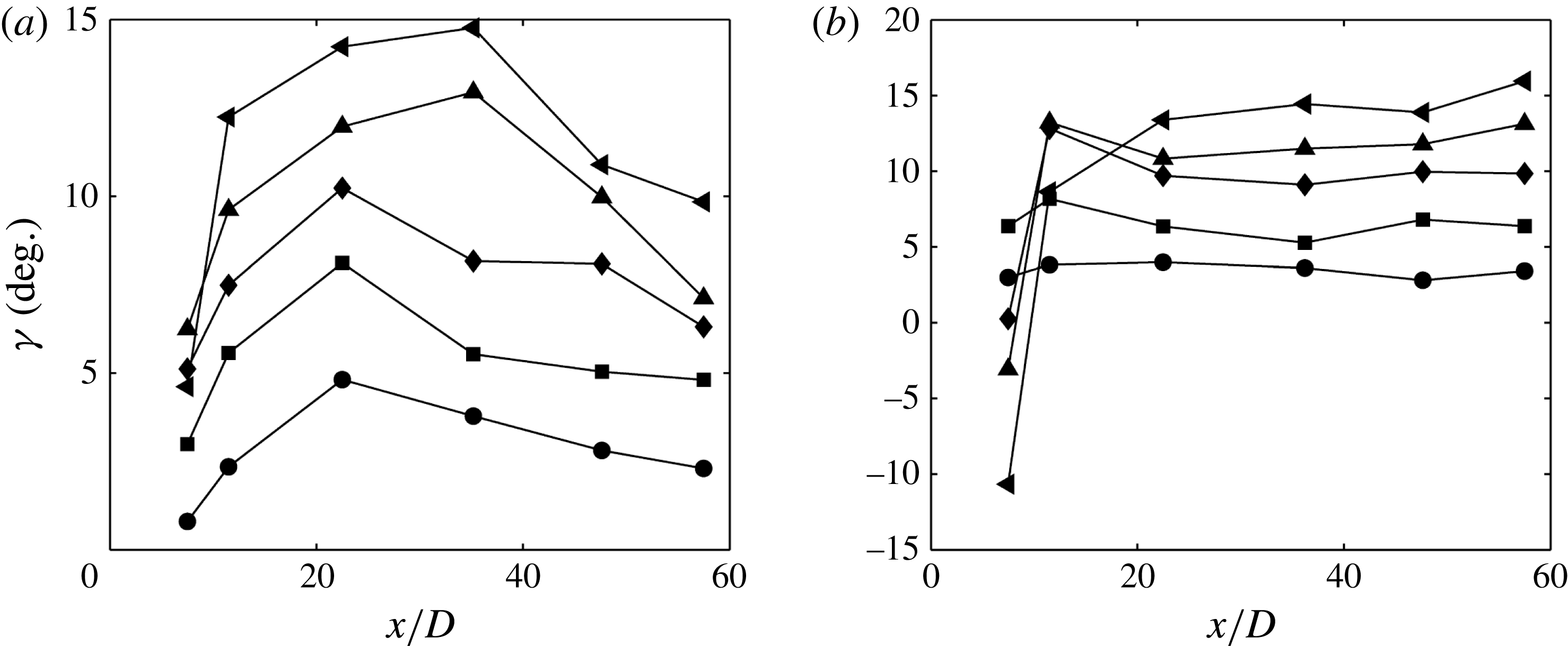
Streamwise variation of the inclination angle of the LCS at different wall-normal heights. (a) Variations of
 ${\it\gamma}$
at physical
 $y$
coordinates: ●,
 $y/D=0.1$
; ▪,
 $y/D=0.2$
; ♦,
 $y/D=0.3$
; ▴,
 $y/D=0.4$
; ◂,
 $y/D=0.5$
. (b) Variations of
 ${\it\gamma}$
at
 $y$
coordinates normalized by the local displacement thickness
 ${\it\delta}_{1}$
: ●,
 $y/{\it\delta}_{1}=1$
; ▪,
 $y/{\it\delta}_{1}=2$
; ♦,
 $y/{\it\delta}_{1}=3$
; ▴,
 $y/{\it\delta}_{1}=4$
; ◂,
 $y/{\it\delta}_{1}=5$
.

In order to show more clearly the change of
 ${\it\gamma}$
in the near-wall region, the streamwise variations of
 ${\it\gamma}$
at five fixed wall-normal heights are presented in figure 14(a). The selected heights (with the largest value of
 $y/D$
being 0.5) are all inside the boundary layer from the beginning of transition to turbulence. As mentioned earlier,
 ${\it\gamma}$
increases until a peak is reached in the middle stage of transition. The streamwise variation of
 ${\it\gamma}$
in the near-wall region is consistent with the evolution of the LCS described in §§ 3.2.1 and 3.2.2. When the secondary vortices destabilize into streamwise elongated
 ${\it\Lambda}$
vortices, the heads of the
 ${\it\Lambda}$
vortices will rise up, resulting in an increase of the inclination angle. This rising-up process continues until the formation of primary hairpin vortices in the transitional boundary layer, where the hairpin vortex heads have moved quite far away from the wall (see figures 5 and 8). Further downstream, however, the formation of large-scale hairpin packets leads to very long streamwise coherent structures (see the streamwise tilted shear layer near the wall shown in figures 9 and 10). These very long structures usually have smaller inclination angles than do the streamwise tilted legs of a single hairpin vortex. This results in decrease of
 ${\it\gamma}$
in the near-wall region.
Figure 14(b) shows the variations of
 ${\it\gamma}$
at five fixed wall-normal heights when the
 $y$
coordinates are normalized by the local displacement thickness
 ${\it\delta}_{1}$
(here
 ${\it\delta}_{1}=\int _{0}^{{\it\delta}}(1-U/U_{{\it\delta}})\,\text{d}y$
, with
 $U_{{\it\delta}}$
being the mean velocity at the boundary layer edge
 ${\it\delta}$
). Note that
 $D$
is a constant while
 ${\it\delta}_{1}$
is changing with the streamwise coordinates. In the initial transition stage (
 $x/D<10$
), the formation of secondary vortices results in a large displacement thickness; so some of the selected points at this streamwise location may be outside the boundary layer and thus reflect the influence of the wake, which can be seen from the negative value of
 ${\it\gamma}$
at the first streamwise location. After
 $x/D>20$
, however, the selected points all fall inside the boundary layer, and
 ${\it\gamma}$
seems to be constant for a fixed
 $y/{\it\delta}_{1}$
. This suggests that the inclination angle of LCS may be scaled from transition to turbulence when normalized with the displacement thickness of the boundary layer.
3.2.4 Near-wall flow structures
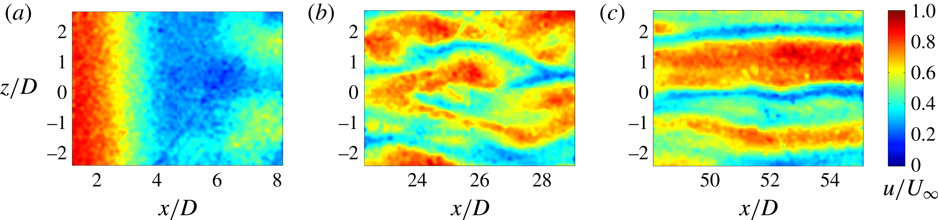
Instantaneous streamwise velocity distributions in the plan view (streamwise–spanwise) plane are shown in figure 15. The measured plane was fixed at
 $y/D=0.15$
in the boundary layer. Figure 15(a) shows the region where the formation and destabilization of the secondary vortices occur. Due to the formation of the secondary vortex, large deceleration can be observed for
 $x/D=2{-}4$
. The good two-dimensionality of the velocity distribution before
 $x/D=4$
is in accordance with the visualization of vortex tubes in figure 4. Downstream of
 $x/D=6$
, the alternate appearance of high- and low-speed regions in the spanwise direction is the result of spanwise destabilization of the secondary vortex. Low-speed streaks in the middle stage of transition can be seen in figure 15(b). These low-speed streaks are probably induced by the streamwise legs of hairpin vortices. The low-speed streaks also appear in the turbulent boundary layer (figure 15
c), but they have a larger streamwise length scale (extending out of view), which can be attributed to the existence of hairpin packets or VLSM. In fact, Adrian (Reference Adrian2007) have already pointed out that the quasi-streamwise legs of individual hairpins are relatively short in comparison with the long streaks in the turbulent boundary layer, but the packets are much longer and can create these long low-speed streaks.
Instantaneous streamwise velocity distributions in the boundary layer in the plane parallel to the wall: (a) at the beginning of transition; (b) in the middle stage of transition; (c) in the turbulent boundary layer. The measured plane was fixed at
 $y/D=0.15$
, which corresponds to approximately
 $y^{+}=9.7$
in (c). The velocity has been normalized by
 $U_{\infty }$
.

Spanwise correlation of streamwise velocity fluctuations: (a)
 $x/D=7.5$
; (b)
 $x/D=25$
; (c)
 $x/D=50$
. The measurements were made at a fixed wall-normal height of
 $y/D=0.15$
. At
 $x/D=50$
, this wall-normal height corresponds to
 $y^{+}=9.75$
. The solid red line in (c) represents the spanwise correlation of streamwise velocity fluctuations in a turbulent channel flow at
 $y^{+}=10.52$
for
 $Re_{{\it\tau}}=180$
(Kim, Moin & Moser Reference Kim, Moin and Moser1987).

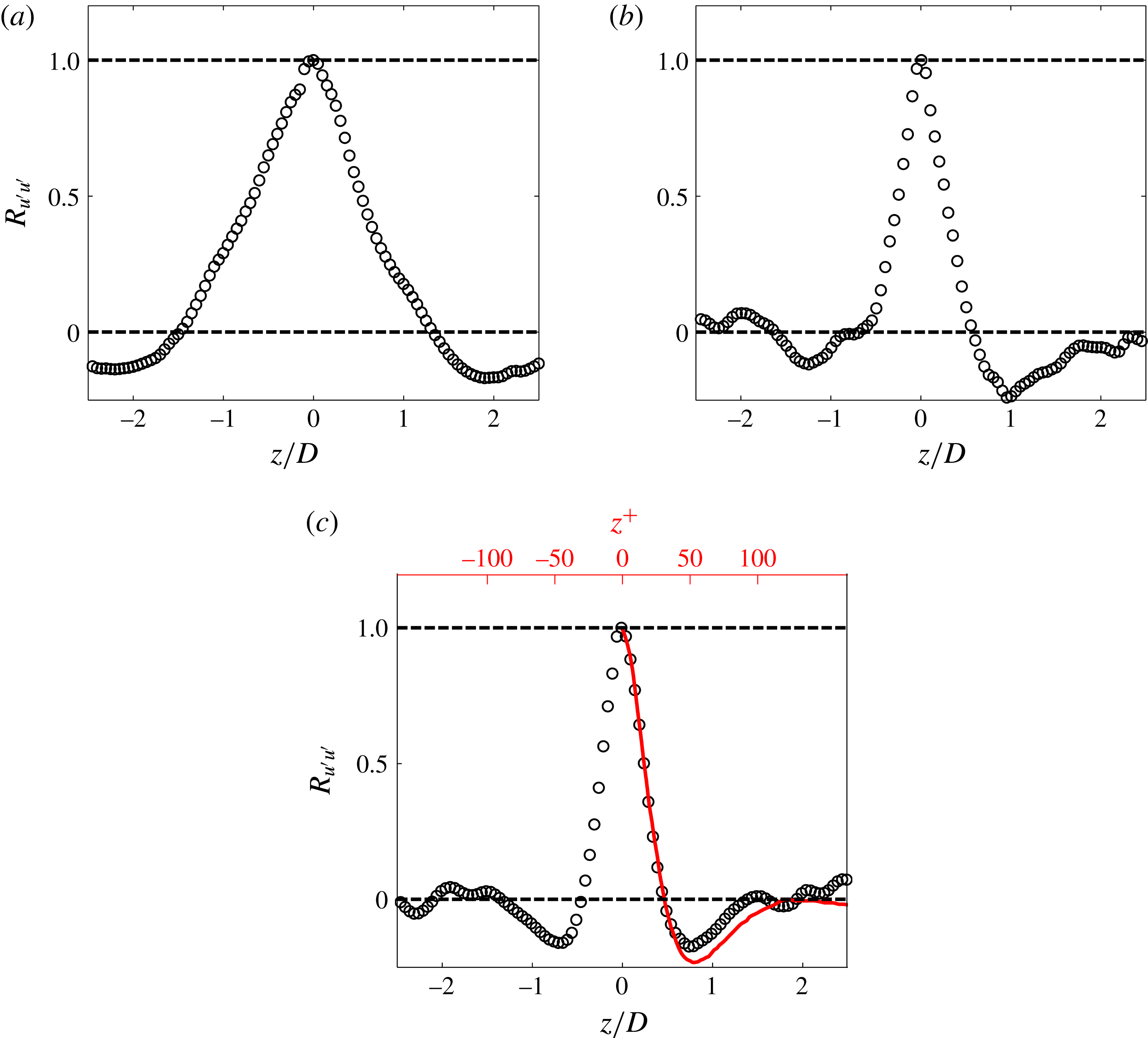
Figure 16 shows the spanwise correlation coefficient of streamwise velocity fluctuations measured in the plan view plane at three streamwise locations. At
 $x/D=7.5$
(figure 16
a), the correlation coefficient shows a spanwise wavelength of approximately
 ${\it\lambda}_{z}=4D$
, in agreement with the spanwise wavelength of
 ${\it\Lambda}$
vortices visualized in figure 4. At the present Reynolds number,
 $4D$
is approximately the spanwise wavelength of the three-dimensional deformation developing on the wake vortices (Williamson Reference Williamson1996). This further proves that the three-dimensional destabilization of the secondary vortex is triggered by perturbations from the wake. At
 $x/D=25$
(figure 16
b), the correlated spanwise wavelength decreases to approximately
 ${\it\lambda}_{z}=2.2D$
, meaning that the spacing of low-speed streaks becomes smaller. At
 $x/D=50$
, the spanwise wavelength decreases to approximately
 ${\it\lambda}_{z}=1.7D$
, corresponding to an inner-scale normalized wavelength of approximately
 ${\it\lambda}_{z}^{+}=96$
, which is very close to the well-established value of approximately 100 for a turbulent boundary layer (Kim et al.
Reference Kim, Moin and Moser1987). This confirms that the turbulent state is reached at
 $x/D=50$
. In their numerical simulation, Ovchinnikov et al. (Reference Ovchinnikov, Piomelli and Choudhari2006) also reported a decrease in spacing of low-speed streaks during transition. The decrease in streak spacing implies a growing population of hairpin vortices and hairpin packets in the boundary layer. According to Asai, Minagawa & Nishioka (Reference Asai, Minagawa and Nishioka2002), the varicose instability of low-speed streaks can lead to the formation of new hairpins. Pan et al. (Reference Pan, Wang, Zhang and Feng2008) claimed that this provides a feedback mechanism to strengthen the regeneration process of hairpin packets. In this way, a self-sustained turbulent boundary layer is eventually established, with hairpin packets prevailing in the outer part of the boundary layer while streaky structures occupy the inner part.
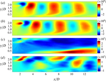
The first four POD modes of the streamwise velocity at the beginning of transition. Panels (a–d) correspond to modes 1–4, respectively.

3.3 Decomposition of the flow field
The above results show that large coherent structures are the dominant structures in the wake-induced boundary layer transition. As we have discussed, the POD method is suitable for extracting such dominant structures. The POD modes of the streamwise velocity component at the beginning of transition are presented in figure 17. The first and second modes form a conjugate pair. The alternate appearance of positive (red) and negative (blue) regions in the wake corresponds to the lower wake vortices. It should be noted here that the secondary vortex induced by the wake vortex is also contained in these first two modes, but it is much weaker than the wake vortex. However, the trace of the secondary vortex can still be seen in the near-wall region as a tail of the coherent structure retarded by the shear layer. What is interesting is the third mode, with a very long mode shape in the near-wall region. This mode corresponds to the evolution of secondary vortices in the boundary layer. The counter-rotating legs of
 ${\it\Lambda}$
vortices can induce low-speed regions between them, which could appear like the third mode in the side view plane. However, the streamwise length of the mode shape is much larger than that of a single
 ${\it\Lambda}$
vortex, so it may represent the influences of a succession of
 ${\it\Lambda}$
vortices (see figures 4 and 7). This suggests that one should be cautious when relating POD mode shape to flow structures. This mode with a streamwise elongated shape in the near-wall region has also been reported by He et al. (Reference He, Wang and Pan2013) using the DMD method (Schmid Reference Schmid2010). Their results showed that the streamwise elongated modes associated with
 ${\it\Lambda}$
vortices were in the low-frequency band and were dominant in terms of disturbance growth. In figure 17(c), we do find that the maximum disturbance (the darkest red region on the POD mode) in this mode shape appears around
 $x/D=10$
, in agreement with the
 $u_{rms.max}$
peak in figure 3(a). Considering that the POD is based on ‘energy’, this confirms again that the low-frequency disturbances are dominant after the three-dimensional destabilization of the secondary vortices into
 ${\it\Lambda}$
vortices. In figure 18(d), the shape of this mode is less organized than the previous ones, and it may be difficult to interpret the physical meaning.
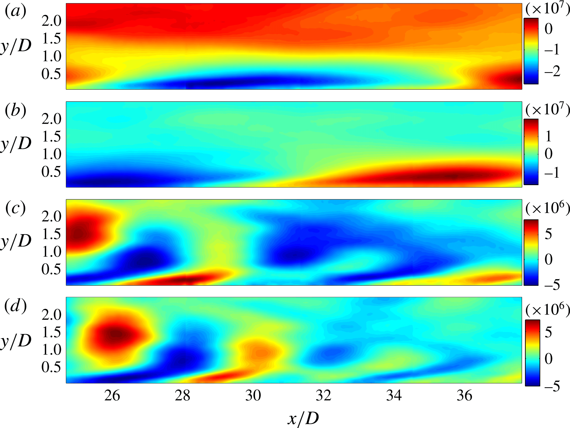
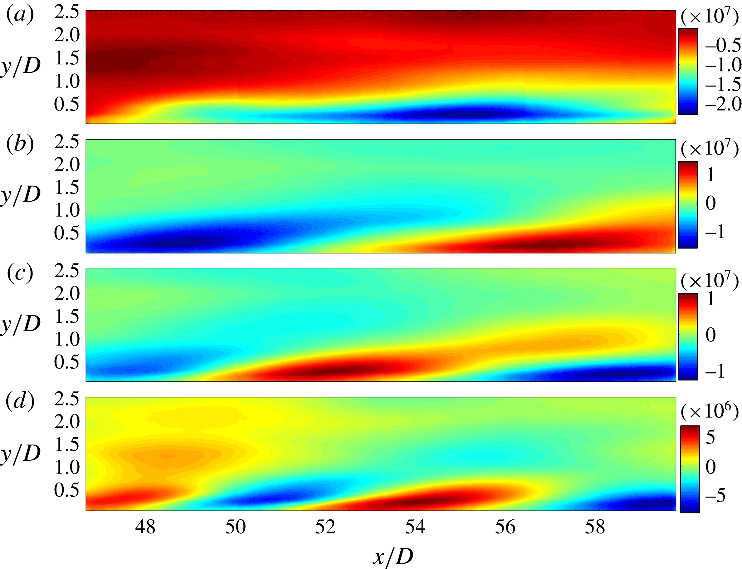
The first four POD modes of the streamwise velocity in the middle stage of transition. Panels (a–d) correspond to modes 1–4, respectively.

Figure 18 displays the POD modes in the middle stage of transition. It is obvious that the first mode is characterized by a long structure inside the boundary layer. It looks similar to the third mode in figure 17(c). At this streamwise location, the legs of the hairpin vortex may play an important role in the inducement of the low-speed regions. The second mode is similar to the first mode but with smaller streamwise length. The outer regions in the third and fourth modes again represent the lower wake vortices. It can be seen that at this streamwise location, the coherency of the wake vortex is not as good as it is in figure 17(a,b); it decays very fast and becomes almost indistinguishable at the end of this FOV. In the near-wall region, some streamwise elongated structures can also be found, but with an even smaller length scale than in the first two modes.
Figure 19 presents the POD modes of the turbulent boundary layer. At this stage, the coherent structures close to the wall are dominant. This is in agreement with the much higher disturbance level in the near-wall region shown in figure 2(l) at
 $x/D=50$
. The POD modes show clearly the decreasing size of streamwise elongated structures in the boundary layer for these four modes. In fact, some similar structures with even smaller streamwise scale can be found in higher-order modes (though for brevity they are not shown here). This variation in scales is very interesting and may well be related to the hierarchy of streamwise scales of LCS in the turbulent boundary layer (figures 9 and 10). Although it is difficult to determine the flow structure behind each mode, it may be reasonable to conjecture that the first mode is related to the VLSM, while the higher modes are related to hairpin packets and hairpin vortices. The results here give more evidence in support of the previous discussion on hierarchy of scales of LCS in the turbulent boundary layer, which was proposed by Adrian and coworkers (Kim & Adrian Reference Kim and Adrian1999; Balakumar & Adrian Reference Balakumar and Adrian2007).
The first four POD modes of the streamwise velocity in the turbulent boundary layer. Panels (a–d) correspond to modes 1–4, respectively.

3.4 Interaction between the large- and small-scale structures
As the turbulent boundary layer contains an abundance of coherent structures with different scales, here we examine an aspect of the interaction between the large- and small-scale structures, following the procedure of Mathis et al. (Reference Mathis, Hutchins and Marusic2009). The procedure has been described in § 2.2.2, and an example is shown here in figure 20. Figure 20(a) gives the streamwise velocity fluctuation
 $u$
at a point in the viscous sublayer (
 $x/D=50$
,
 $y^{+}=7$
), and significant low-frequency fluctuations can be seen, as expected. The streamwise velocity fluctuation
 $u$
is decomposed into a large-scale component
 $u_{L}$
and a small-scale component
 $u_{S}$
(shown in figure 20
b) by a cutoff frequency
 $f_{c}$
. In the present work, a crude estimation of the boundary layer turnover time
 $T_{t}$
(
 $T_{t}={\it\delta}/U_{\infty }$
, with
 ${\it\delta}$
set to
 $2.5D$
here) is 0.75 s, corresponding to a frequency of approximately 1.33 Hz. As Mathis et al. (Reference Mathis, Hutchins and Marusic2009) mentioned that the modulation is not sensitive to the choice of
 $f_{c}$
over a wide range,
 $f_{c}$
is chosen to be a rounded value of 1.5 Hz in this investigation. It is assumed that structures with streamwise wavelengths larger than the boundary layer thickness are within
 $u_{L}$
. The low-pass filtered envelope
 $E_{L}(u_{S})$
is obtained by applying the Hilbert transformation to
 $u_{S}$
, followed by a low-pass filtering;
 $u_{S}$
and its envelope
 $E_{L}(u_{S})$
are plotted together in figure 20(c). It can be seen that
 $E_{L}(u_{S})$
rises up where large-amplitude fluctuations of
 $u_{S}$
are present (for example, at approximately
 $t=40$
s). In figure 20(d),
 $E_{L}(u_{S})$
and
 $u_{L}$
are plotted together; they show a strong positive correlation, indicating the influence of large-scale amplitude modulation on small-scale structures.
(a) Fluctuation of streamwise velocity
 $u$
at
 $x/D=50$
and
 $y^{+}=7$
; the fluctuation velocity has been normalized by the free-stream velocity
 $U_{\infty }$
. (b) The large-scale component
 $u_{L}$
(dashed line) and the small-scale component
 $u_{S}$
(solid line). (c) The envelope
 $E_{L}(u_{S})$
(thick red line) of
 $u_{S}$
(thin black line). (d) Plots of
 $E_{L}(u_{S})$
(red solid line) and
 $u_{L}$
(black dashed line); to facilitate comparison, the mean of
 $E_{L}(u_{S})$
was adjusted to zero and its magnitude was magnified by a factor of 10.

The modulation effect of large structures on small structures across the boundary layer is shown in figure 21(a). The trend of the curve generally follows the result of Mathis et al. (Reference Mathis, Hutchins and Marusic2009): in the near-wall region, a high positive correlation coefficient indicates that the large coherent structures in the turbulent boundary layer exert a high modulation on the small structures very close to the wall. This modulation decreases with increase of the wall-normal height, and at
 $y^{+}=18$
the correlation coefficient drops to zero. This location is very close to
 $y_{peak}^{+}=16$
, where
 $u_{rms.max}$
reaches its maximum value in the turbulent boundary layer. Further away from the wall, the correlation turns negative and then increases to positive again in the outer region where the influence of the wake may be present. It should be pointed out that the correlation in the present study (especially the negative correlation peak) is lower than that reported by Mathis et al. (Reference Mathis, Hutchins and Marusic2009). This can be attributed to the much lower Reynolds number in the present study. The velocity profile of the turbulent boundary layer is presented in figure 21(b). Close to the wall, the profile agrees very well with a Spalding fit. In the outer region, however, the turbulent log region cannot be seen. This is because the boundary layer Reynolds number is low, and the wake of the cylinder still causes a deficit of flow velocity (shown in figure 2 f at
 $x/D=50$
). As the current boundary layer Reynolds number is much lower than that in the study of Mathis et al. (Reference Mathis, Hutchins and Marusic2009), no well-defined ‘superstructure’ (or VLSM) should be expected. However, it has been shown that the coherent alignment of hairpin vortices tends to form a very large structure (figure 10), similar to the formation of VLSM at high Reynolds number. As a result, similar modulations are observed at low Reynolds number in the present wake-induced transition scenario.
(a) Amplitude modulation of the small-scale structures at
 $x/D=50$
. (b) Mean boundary layer profile at
 $x/D=50$
; blue stars represent measured data. The log-law expression used here is
 $U^{+}=2.439\ln (y^{+})+5.5$
(the inclined dashed straight line). The red solid line is the Spalding fit (Kendall & Koochesfahani Reference Kendall and Koochesfahani2006). The vertical dashed line indicates the wall-normal location where
 $R$
equals zero in (a).

4 Conclusions
The evolution of LCS in a flat plate boundary layer transition induced by the wake of a circular cylinder is experimentally investigated using both hydrogen bubble visualization and PIV techniques. The characteristics of the mean velocity and the coherent structures are examined.
Mean velocity statistics show a fast disturbance growth inside the boundary layer immediately downstream of the cylinder, corresponding to the formation and destabilization of the secondary vortices. After reaching a maximum at around
 $x/D=10$
, the disturbance level begins a slow decay and eventually reaches a nearly stable level for
 $x/D>35$
, where the turbulent boundary layer is fully developed. The location of
 $u_{rms.max}$
is found to increase in the wall-normal direction corresponding to the fast disturbance growth, which results from the local separation associated with the formation of secondary vortices.
The evolution of the LCS, from the very beginning of transition up to when the boundary layer becomes turbulent, is revealed both by hydrogen bubble visualizations and FTLE fields. The mean convection velocity and average inclination angle of the LCS can be extracted from the quantitative FTLE fields. The mean convection velocity of the LCS agrees with the local mean Eulerian velocity when the boundary layer becomes fully developed turbulent flow, except that it is always higher than the latter in the near-wall region where viscosity is dominant. It is shown that the present definition of inclination angle based on correlation of FTLE fields in a two-dimensional plane eliminates bias errors arising from hot-wire measurements. The average inclination angle of LCS in the boundary layer increases at the beginning and then decreases. This is consistent with the observed formation of hairpin vortices and hairpin packets, respectively. However, when the wall-normal height is normalized with the local displacement thickness, the inclination angle at a fixed height seems to be constant after
 $x/D>20$
. This suggests that there may be a scaling law of the average inclination angle of LCS with respect to the outer length scale of the boundary layer from transition to turbulence. However, more evidence will be needed to corroborate this observation.
The measurements made on the plan view plane close to the wall show that after the spanwise destabilization of secondary vortices, streamwise elongated low-speed regions begin to appear in the boundary layer. In the middle stage of boundary layer transition, where hairpin vortices have formed, low-speed streaks can be observed close to the wall, which are the result of inducement of the hairpin vortex legs. Further downstream in the turbulent boundary layer, the low-speed streaks have larger streamwise scale, due to the formation of hairpin packets (figure 9) or VLSM (figure 10). The spanwise correlation of the velocity fluctuations reveals a spanwise wavelength of approximately
 ${\it\lambda}_{z}=4D$
for the
 ${\it\Lambda}$
vortices, in agreement with the spanwise wavelength of mode-A instability developing along the wake vortices (Williamson Reference Williamson1996). This demonstrates that the three-dimensional destabilization of the secondary vortices is triggered by the wake disturbances. The spanwise correlation also shows that the average distance of low-speed streaks decreases during transition, which is in accordance with the growing population of hairpin vortices and hairpin packets in the boundary layer.
The POD modes show the decay of wake vortices in the outer region, while in the boundary layer the streamwise elongated mode shape is present since the spanwise destabilization of the secondary vortices. POD modes of the turbulent boundary layer reveal a variety of scales of streamwise elongated structures, in accordance with the hierarchy of scales exhibited by hairpin vortices, hairpin packets and VLSM. A correlation between the low-frequency fluctuations and the low-pass filtered envelope of the high-frequency fluctuations shows that the large-scale structures in the boundary layer can modulate the amplitude of the small-scale structures near the wall at the low Reynolds number used in the present study.
Acknowledgements
This work was supported by the National Natural Science Foundation of China (grant nos 11327202, 11490552 and 11502011). It was also funded by the China Postdoctoral Science Foundation (2015M570023).
Supplementary movies
Supplementary movies are available at http://dx.doi.org/10.1017/jfm.2016.81.