


1 Introduction
1.1 Representations
Let
$\mathbb {S}_4^2$
 denote the two-dimensional sphere with four punctures. A presentation of its fundamental group is

where the generators
$\alpha $
 ,
$\beta $
 ,
$\gamma $
 ,
$\delta $
 correspond to disjoint simple loops around the punctures (see Figure 1, taken from [Reference Cantat and Loray19]). Thus,
$\pi _1(\mathbb {S}_4^2)$
 is the free group on the three generators
$\alpha $
 ,
$\beta $
 , and
$\gamma $
 .
Let
${\textsf {Rep}}(\mathbb {S}_4^2)$
 be the set of representations of
$\pi _1(\mathbb {S}_4^2)$
 in
${\textsf {SL}}_2(\mathbb {C})$
 . Such a representation
$\rho $
 is uniquely determined by the three matrices
$\rho (\alpha )$
 ,
$\rho (\beta )$
 ,
$\rho (\gamma )$
 , so that
${\textsf {Rep}}(\mathbb {S}_4^2)$
 can be identified with
${\textsf {SL}}_2(\mathbb {C})^3$
 . As in [Reference Benedetto and Goldman2, Reference Cantat and Loray19], we associate the following traces to such a representation:


Then the polynomial map
$\chi \colon {\textsf {Rep}}(\mathbb {S}_4^2)\to \mathbb {A}^7(\mathbb {C})$
 defined by

is invariant under conjugacy, its image is the hypersurface determined by the equation

with


and
$\chi $
 is the quotient map for the action of
${\textsf {SL}}_2(\mathbb {C})$
 on
${\textsf {Rep}}(\mathbb {S}_4^2)$
 by conjugacy, in the sense of invariant theory. We shall denote the character variety
${\textsf {Rep}}(\mathbb {S}_4^2)/\!\!/{\textsf {SL}}_2(\mathbb {C})$
 by
$\chi (\mathbb {S}_4^2)$
 (instead of
$\chi ({\textsf {Rep}}(\mathbb {S}_4^2))$
 ).
Fundamental group of the two-dimensional sphere with four punctures (color online).

For each choice of parameters A, B, C, D, we shall denote by
$S_{(A,B,C,D)}$
 the algebraic surface determined by equation (1.5); it is a cubic surface in the affine space
$\mathbb {A}^3$
 , of degree
$2$
 with respect to each variable x, y, or z. The family of all these surfaces will be denoted by
${\textsf {Fam}}$
 . For simplicity, we shall just write S instead of
$S_{(A,B,C,D)}$
 for the elements of
${\textsf {Fam}}$
 (the quadruple
$(A,B,C,D)$
 is then uniquely determined by S). If the parameters A, B, C, and D are in a ring R, we denote by
$S(R)$
 the points of S with coordinates in R.
The compactification of S in the projective space
$\mathbb {P}^3$
 will be denoted by
${\overline S}$
 and its boundary at infinity by

For every
$S\in {\textsf {Fam}}$
 ,
$\partial S$
 is the triangle in the hyperplane at infinity given by the equation
$xyz=0$
 .
1.2 Mapping class group and Vieta involutions
Let us view the mapping class group
${\textsf {Mod}}^{\pm }(\mathbb {S}_4^2)$
 as the subgroup of
${\textsf {Out}}(\pi _1(\mathbb {S}_4^2))$
 preserving the peripheral structure. Then
${\textsf {Mod}}^{\pm }(\mathbb {S}_4^2)$
 acts on
$\chi (\mathbb {S}_4^2)$
 by precomposition, the conjugacy class of a representation
$\rho $
 being sent to the conjugacy class of
$\rho \circ \Phi ^{-1}$
 for any mapping class
$\Phi $
 . This gives a homomorphism
$\Phi \mapsto f_\Phi $
 into the group
${\textsf {Aut}}(\chi (\mathbb {S}_4^2))$
 of automorphisms of the variety
$\chi (\mathbb {S}_4^2)$
 . As explained in [Reference Cantat and Loray19, §§2.2 and 2.3], there is an isomorphism

where H is the group
$(\mathbb {Z}/2\mathbb {Z})^2$
 , and an exact sequence

where
${\text {Sym}}(4)$
 corresponds to the group of permutation of the four punctures of
$\mathbb {S}_4^2$
 and
$\Gamma ^{\pm }_2$
 is the congruence subgroup of
${\textsf {PGL}}_2(\mathbb {Z})$
 modulo
$2$
 :
-
(1) $\Gamma ^{\pm }_2$
 is isomorphic to
$\mathbb {Z}/2\mathbb {Z}\star \mathbb {Z}/2\mathbb {Z}\star \mathbb {Z}/2\mathbb {Z}$
, generated by the three involutions (1.11) $$ \begin{align} \hat\sigma_x=\bigg(\begin{array}{cc} -1 & 2 \\ 0 & 1\end{array}\bigg), \quad \hat\sigma_y=\bigg(\begin{array}{cc} 1 & 0 \\ 2 & -1\end{array}\bigg) , \quad \hat\sigma_z=\bigg(\begin{array}{cc} 1 & 0 \\ 0 & -1\end{array}\bigg); \end{align} $$
-
(2) $\Gamma ^{\pm }_2$
is the reflection group of an ideal triangle in the upper half plane; -
(3) the action of $\Gamma ^{\pm }_2$
on the character variety
$\chi (\mathbb {S}_4^2)$
preserves the four coordinates a, b, c, d; in particular, it acts on each surface
$S\in {\textsf {Fam}}$
as a group of automorphisms of S; this action is faithful for every S, and the image has index at most
$24$
in
${\textsf {Aut}}(S)$
(see [Reference Cantat and Loray19, Theorem 3.1]); -
(4) the image of $\Gamma ^{\pm }_2$
in
${\textsf {Aut}}(S)$
is generated by the Vieta involutions (1.12) $$ \begin{align} s_x(x,y,z)&=(-x-yz+A, y, z), \notag \\ s_y(x,y,z)&=(x, -y-zx+B, z), \\ s_z(x,y,z)&=(x, y, -z-xy+C).\notag \end{align} $$


In what follows, we denote by
$\Gamma $
 the abstract group
$\mathbb {Z}/2\mathbb {Z}\star \mathbb {Z}/2\mathbb {Z}\star \mathbb {Z}/2\mathbb {Z}$
 . Depending on the action we look at,
$\Gamma $
 will determine a subgroup
$\Gamma ^{\pm }_2$
 of isometries of the upper half plane, or a group of automorphisms
$\Gamma _S$
 of S (for any S in
${\textsf {Fam}}$
 ). Our goal is to describe the stochastic dynamics of this action on each of the surfaces S. For simplicity, we frequently write
$\Gamma $
 instead of
$\Gamma _S$
 .
1.3 Invariant area form
On S, the
$2$
 -form

is regular and does not vanish. According to Lemma 3.5 of [Reference Cantat and Loray19], singularities of S are quotient singularities, and
${\mathrm {Area}}$
 is an area form in the sense of orbifolds (locally, in a Euclidean neighborhood of the singularity, S is the quotient
$\mathbb {C}^2/G$
 for some finite group and
${\mathrm {Area}}$
 is the quotient of a G-invariant symplectic
$2$
 -form on
$\mathbb {C}^2$
 ).
When S is defined over
$\mathbb {R}$
 ,
${\mathrm {Area}}$
 is also defined over
$\mathbb {R}$
 . To distinguish between the holomorphic
$2$
 -form on
$S(\mathbb {C})$
 and the real
$2$
 -form on
$S(\mathbb {R})$
 , we use the notation
${\mathrm {Area}}_{\mathbb {C}}$
 and
${\mathrm {Area}}_{\mathbb {R}}$
 .
The
$2$
 -form
${\mathrm {Area}}_{\mathbb {C}}$
 (respectively,
${\mathrm {Area}}_{\mathbb {R}}$
 ) is multiplied by
$-1$
 under the action of each of the involutions
$s_x$
 ,
$s_y$
 ,
$s_z$
 .
When S is defined over
$\mathbb {R}$
 ,
$S(\mathbb {R})$
 may have a compact connected component; we denote such a component by
$S(\mathbb {R})_c$
 (see §2.2 for a precise definition when S is singular). With our notation, it may happen that
$S(\mathbb {R})_c$
 is reduced to a point; otherwise, it is a (possibly singular) sphere and the restriction of
${\mathrm {Area}}_{\mathbb {R}}$
 to
$S(\mathbb {R})_c$
 determines (a) an orientation of this sphere and (b) a probability measure
$\nu _{\mathbb {R}}$
 on
$S(\mathbb {R})_c$
 , defined by

for any Borel subset B of
$S(\mathbb {R})_c$
 . We shall refer to this measure as the symplectic measure on
$S(\mathbb {R})_c$
 . It is
$\Gamma _S$
 -invariant.
1.4 Random dynamics
Let X be a locally compact metric space. We endow the group
${\textsf {Homeo}}(X)$
 with the compact-open topology. Let
$\mu $
 be a probability measure on
${\textsf {Homeo}}(X)$
 . Denote by
$\Omega $
 the product space
${\textsf {Homeo}}(X)^{\mathbb {N}}$
 and endow it with the probability measure
$\mu ^{\mathbb {N}}$
 . We shall say that a property holds for a typical element
$\omega \in \Omega $
 if it holds for
$\omega $
 in a measurable subset
$\Omega '$
 with
$\mu ^{\mathbb {N}}(\Omega ')=1$
 . For every
$\omega = (f_0,f_1,\ldots ) \in \Omega $
 , we set

A probability measure
$\nu $
 on X is
$\mu $
 -stationary if

and such a measure is ergodic if it cannot be written as a convex combination of two distinct stationary measures. Fix a point q in X. Then consider the random orbit
$(f_\omega ^n(q))$
 and the empirical measures

A theorem of Breiman (see [Reference Benoist and Quint3]) says that, for a subset of measure
$1$
 in
$\Omega $
 , if
$\nu _{n_i}(\omega; q)$
 converges towards a probability measure
$\nu $
 as
$n_i$
 goes to infinity, then
$\nu $
 is
$\mu $
 -stationary. Thus, to understand how random orbits distribute, we have to describe stationary measures. We apply this viewpoint to the dynamics of
$\Gamma _S$
 .
Main Theorem. Let
$\mu $
 be a probability measure on
$\{s_x,s_y,s_z\}$
 with

Let S be an element of
${\textsf {Fam}}$
 . Let
$\nu $
 be a probability measure on
$S(\mathbb {C})$
 . If
$\nu $
 is
$\mu $
 -stationary and ergodic, then the support of
$\nu $
 is compact,
$\nu $
 is invariant, and either
$\nu $
 is given by the average on a finite orbit of
$\Gamma _S$
 , or:
-
• the parameters A, B, C, and D defining S are real and in $[-2,2]$
; -
• $S(\mathbb {R})$
has a unique bounded component
$S(\mathbb {R})_c$
, of dimension
$2$
; and -
• $\nu $
coincides with the symplectic measure
$\nu _{\mathbb {R}}$
induced by
${\mathrm {Area}}_{\mathbb {R}}$
on
$S(\mathbb {R})_c$
.


This extends a result of Chung for the dynamics on the compact part
$S(\mathbb {R})_c$
 when
$(A,B,C,D)=(0,0,0,D)$
 with
$D\in [3.9,4]$
 (see [Reference Chung20, Theorem B]).
Since finite orbits have been classified, our Main Theorem gives a complete description of all
$\mu $
 -stationary measures. In particular:
-
• on each surface $S\in {\textsf {Fam}}$
, except on
$S_{(0,0,0,4)}$
, the set of
$\mu $
-stationary measures is a finite-dimensional simplex with at most six vertices, the maximum six being realized only by
$S_{(0,0,0,3)}$
; -
• if $S(\mathbb {R})$
has a compact component
$S(\mathbb {R})_c$
that does not contain any finite orbit, then given any
$q\in S(\mathbb {R})_c$
, the empirical measures
$\nu _N(\omega ;q)$
almost surely converge to the symplectic measure
$\nu _{\mathbb {R}}$
as N goes to
$+\infty $
.


Our result certainly holds when the support of
$\mu $
 generates the group
$\Gamma $
 and satisfies an exponential moment condition. We wrote the proof assuming that the support is equal to
$ \{ s_x, s_y, s_z \}$
 for two reasons. First, all essential difficulties already appear in this case. (For instance, when one compactifies S, the elements of
$\Gamma _S$
 have indeterminacy points at infinity. Since the support of
$\mu $
 generates
$\Gamma _S$
 , all these indeterminacies appear in our study.) Second, this simplifies the exposition because it allows us to avoid some aspects of the general theory of random walks on
$\Gamma $
 .
1.5 Previous works
We do not need the results contained in [Reference Cantat14, Reference Cantat and Jang18, Reference Iwasaki and Uehara24, Reference Rebelo and Roeder29], but those three papers are closely related to the present work, in particular [Reference Rebelo and Roeder29] for its study of the Julia/Fatou dichotomy for the action of
$\Gamma _S$
 on
$S(\mathbb {C})$
 , and [Reference Cantat and Jang18] for the action of
$\Gamma _S$
 on
$S(\mathbb {Q}_p)$
 , when A, B, C, and D are p-adic numbers. See also [Reference Nerrière27] for the case of polynomial automorphisms of
$\mathbb {C}^2$
 .
2 The Markov surfaces and their automorphisms
2.1 Smoothness of
$S(\mathbb {C})$

In [Reference Benedetto and Goldman2], Benedetto and Goldman study the topology of the surfaces
$S\in {\textsf {Fam}}$
 . Their first result says that S is singular if and only if at least one of the parameters a, b, c, or d is equal to
$\pm 2$
 or there is a reducible representation with boundary traces a, b, c, d. Moreover, the latter case occurs if and only if the following discriminant vanishes:

Example 2.1. The Cayley cubic
$S_{\mathrm {Ca}}=S_{(0,0,0,4)}$
 is defined by the equation
$x^2+y^2+z^2+xyz=4$
 . It has four singularities, the maximum for an irreducible cubic surface. It is the quotient of the multiplicative group
${\mathbb {G}}_m\times {\mathbb {G}}_m$
 by
$\eta (u,v)=(1/u,1/v)$
 , the quotient map being

2.2 Topology of
$S(\mathbb {R})$

Let n be the number of boundary traces a, b, c, d in the interval
$[-2,2]$
 . From [Reference Benedetto and Goldman2, Theorem 1.2], we deduce that if
$S(\mathbb {R})$
 is smooth, then its Euler characteristic is equal to
$2n-2$
 and
$S(\mathbb {R})$
 is made of at most five connected components; the maximum five is reached if and only if
$S(\mathbb {R})$
 contains a compact connected component, which is then unique and homeomorphic to a sphere. When S is allowed to have singularities, we define the components of
$S(\mathbb {R})$
 as follows. First, if
$S(\mathbb {R})$
 has an isolated point, this point will be one of the components of
$S(\mathbb {R})$
 ; note that there is at most one isolated point, it must be one of the singularities of
$S(\mathbb {R})$
 , and a well-chosen perturbation of the coefficients
$(a, b, c, d)$
 will turn this point into a small sphere (respectively, will make this point disappear). Second, consider the smooth part
$S(\mathbb {R})\setminus {\textsf {Sing}}(S)$
 , and split it as a disjoint union of connected components
$S(\mathbb {R})_i^0$
 ; then replace each
$S_i^0(\mathbb {R})$
 by its closure (equivalently, add to
$S(\mathbb {R})_i^0$
 the singularities of S which are contained in the closure of
$S(\mathbb {R})_i^0$
 ); the result

will be one of the components of
$S(\mathbb {R})$
 . For instance, in the case of the Cayley cubic,
$S(\mathbb {R})$
 has a compact component: it contains four singularities, each of which is contained in exactly one of the unbounded components.
With this definition at hand, the classification of Benedetto and Goldman remains correct, except that the components are not necessarily disjoint (they may touch at singularities) and the sphere in case (6) can be reduced to a singular point. In particular, one gets the following result: if
$S(\mathbb {R})$
 has a compact component, this component is unique, and it is homeomorphic to a sphere or a singleton. If such a component exists, it will be denoted by
$S(\mathbb {R})_c$
 ; when
$S(\mathbb {R})$
 has an isolated point,
$S(\mathbb {R})_c$
 is equal to this point.
2.3 Representations in the compact component
The group
${\textsf {SL}}_2(\mathbb {C})$
 has two real forms, one is
${\textsf {SL}}_2(\mathbb {R})$
 , the other is
${\textsf {SU}}_2$
 . Since
${\textsf {SU}}_2$
 is compact, representations in
${\textsf {SU}}_2$
 give points in
$S(\mathbb {R})_c$
 ; but points of
$S(\mathbb {R})_c$
 may also correspond to representations in
${\textsf {SL}}_2(\mathbb {R})$
 (see [Reference Benedetto and Goldman2, Proposition 1.4]). In fact, according to [Reference Cantat and Loray19, Lemma 2.7], the map

from equations (1.6) and (1.7) is a ramified cover of degree
$24$
 and
${\mathrm {Jac}}(\Pi )=-\tfrac 12\Delta $
 , where
$\Delta $
 is the discriminant from §2.1. The following automorphisms of
$\mathbb {C}^4$
 generate a group
$Q\subset {\textsf {Aut}}(\mathbb {C}^4)$
 of order
$8$
 :
-
(a) the simultaneous sign change of the parameters a, b, c, and d;
-
(b) the permutations of a, b, c, and d which are a composition of two transpositions with disjoint supports.
The ramified cover
$\Pi $
 is invariant under the action of Q. But
$\Pi $
 is not Galois, and to understand the structure of the
$24$
 points in the fibers of
$\Pi $
 , one has to introduce the Okamoto correspondences (see §3 of [Reference Cantat and Loray19] for this).
If
$S(\mathbb {R})$
 has a compact component, then
$(A,B,C,D)$
 is contained in
$[-2,2]^4$
 and
$\Pi ^{-1}\{(A,B,C,D)\}$
 is also entirely contained in
$[-2,2]^4$
 . Moreover, different choices of
$(a,b,c,d)$
 in
$\Pi ^{-1}\{(A,B,C,D)\}$
 lead to different types of representations, as summarized in the following result (see [Reference Cantat and Loray19, Theorem B and Proposition 3.13]).
Theorem 2.2. Let
$(A,B,C,D)$
 be real parameters. If the smooth part of
$S(\mathbb {R})$
 has a bounded component, then all parameters
$(a,b,c,d)$
 in
$\Pi ^{-1}\{(A,B,C,D)\}$
 are real. Moreover, the points of
$S(\mathbb {R})_c$
 are conjugacy classes of
${\textsf {SU}}_2$
 - and
${\textsf {SL}}_2(\mathbb {R})$
 -representations, depending on the choice of
$(a,b,c,d)$
 : modulo the action of the group Q, each point of
$S(\mathbb {R})_c$
 corresponds to two
${\textsf {SU}}_2$
 -representations and one
${\textsf {SL}}_2(\mathbb {R})$
 -representation.
3 Invariant compact subsets and invariant measures on them
In this section, we summarize some known results concerning
$\Gamma _S$
 -invariant compact subsets of
$S(\mathbb {C})$
 and derive from them a classification of
$\Gamma _S$
 -invariant probability measures on
$S(\mathbb {C})$
 .
3.1 Finite orbits
Boalch [Reference Boalch4–Reference Boalch6] and Lisovyy and Tykhyy [Reference Lisovyy and Tykhyy26] obtained a classification of all finite orbits of
$\Gamma $
 in the surfaces
$S\in {\textsf {Fam}}$
 . We summarize their results.
3.1.1 Short orbits
Orbits of
$\Gamma $
 with at most four elements are classified in [Reference Lisovyy and Tykhyy26, Lemma 39]. They come in families depending on no more than three parameters, up to permutation of the coordinates. Fixed points coincide with singularities of S, and form a three-parameter family; here
$(a,b,c,d)$
 satisfies
$(4-a^2)(4-b^2)(4-c^2)(4-d^2)\Delta \,{=}\,0$
 . Orbits of length
$2$
 depend on two parameters; for instance,
$\{(x,0,0), (x',0,0)\}$
 is such an orbit if
$A=x+x'$
 ,
$B=0$
 ,
$C=0$
 , and
$D=4+x+x'$
 . Orbits of length
$3$
 or
$4$
 depend on one parameter; for a generic choice of it, the orbit corresponds to representations of
$\pi _1(\mathbb {S}_4^2)$
 with infinite image.
3.1.2 Finite groups
Let F be a finite subgroup of
${\textsf {SL}}_2(\mathbb {C})$
 . Each representation of
$\pi _1(\mathbb {S}_4^2)$
 into F gives rise to a finite orbit of
$\Gamma $
 in
$\chi (\mathbb {S}_4^2)$
 . Changing F into a conjugate subgroup of
${\textsf {SL}}_2(\mathbb {C})$
 does not change the corresponding orbit. The finite orbits obtained with this method are described by Boalch in [Reference Boalch4–Reference Boalch8]. Note that changing the parameters
$(a,b,c,d)$
 in
$\Pi ^{-1}(A,B,C,D)$
 may turn a representation inside a finite group into a representation with infinite image.
Example 3.1. Consider the Cayley cubic
$S_{\mathrm {Ca}}=S_{(0,0,0,4)}$
 described in Example 2.1. The group
${\textsf {GL}}_2(\mathbb {Z})$
 acts by monomial transformations on the multiplicative group
${\mathbb {G}}_m(\mathbb {C})\times {\mathbb {G}}_m(\mathbb {C})$
 and each point of type
$(e^{2{\textsf {i}}\pi p/q}, e^{2{\textsf {i}}\pi p'/q'})$
 has a finite orbit for this action. On the other hand, this action commutes to the involution
$\eta $
 and induces a subgroup of
${\textsf {Aut}}(S)$
 that contains
$\Gamma _{S_{\mathrm {Ca}}}$
 as a finite index subgroup (see [Reference Cantat and Loray19]). Thus, their projections

give points on the Cayley cubic with finite
$\Gamma _{S_{\mathrm {Ca}}}$
 -orbits. The Cayley cubic is the unique example of a surface
$S\in {\textsf {Fam}}$
 containing infinitely many finite orbits.
3.1.3 Boalch–Klein orbit
In [Reference Boalch5], Boalch constructs a finite orbit that is not given by any representation to a finite subgroup of
${\textsf {SL}}_2(\mathbb {C})$
 (it comes from a representation into a finite subgroup of
${\textsf {SL}}_3(\mathbb {C})$
 , though). The surface is defined by the equation
$x^2+y^2+z^2+xyz=x+y+z$
 and the orbit includes the seven points
$(0,0,0)$
 ,
$(1,0,0)$
 ,
$(0,1,0)$
 ,
$(0,0,1)$
 ,
$(1,1,0)$
 ,
$(1,0,1)$
 , and
$(0, 1,1)$
 . There are
$24$
 choices of parameters
$(a,b,c,d)$
 giving rise to
$(A,B,C,D)=(1,1,1,0)$
 . One of them is
$a=b=c=2\cos (2\pi /7)$
 ,
$d= 2\cos (4\pi /7)$
 . For such a choice, the image of the representation
$\pi _1(\mathbb {S}_4^2)\to {\textsf {PSL}}_2(\mathbb {C})$
 is conjugate to the triangle group
$T(2,3,7)$
 . The Galois conjugates of this representations provide two distinct representations in
${\textsf {SU}}_2$
 (corresponding to conjugates of a, b, c, d). Modulo Okamoto symmetries, all orbits of length
$7$
 are given by these three representations.
3.1.4 Boalch–Kitaev orbits
Consider the surface
$ x^2 + y^2 + z^2 + xyz= (1 + \alpha )(x + y + z)- 2\alpha $
 where
$\alpha \in \{ 2 \cos (\pi /7), 2\cos (3\pi /7), 2\cos (5\pi /7) \} $
 is one of the roots of the equation
$ t^3=t^2+2t-1$
 . Then the orbit of
$(0,1,1)$
 contains
$18$
 elements. This gives three finite orbits, one for each choice of
$\alpha $
 . It would be nice to interpret these orbits in terms of representations into a finite subgroup of some algebraic group G, as done for the Boalch–Klein orbit with
$G = {\textsf {SL}}_3(\mathbb {C})$
 (see the construction in §5 of [Reference Boalch8] and the problem described in Remark 21 of [Reference Boalch and Paluba9]).
3.1.5 Classification
Lisovyy and Tykhyy proved that every finite orbit of
$\Gamma $
 is given by one of the above examples. The parameters for finite orbits are listed in Lemma 39 on page 147, Theorem 1 on page 149 and Table 4 on page 150 of [Reference Lisovyy and Tykhyy26] (see also [Reference Boalch7]). Points with a finite orbit of length at least
$5$
 are determined by representations of
$\pi _1(\mathbb {S}_4^2)$
 in a finite subgroup of
${\textsf {SU}}_2$
 , except for the Boalch–Klein orbit and the three Boalch–Kitaev orbits.
3.2 Invariant compact subsets and probability measures
From Lemma 4.3 and Theorems B and C of [Reference Cantat and Loray19], one gets the following result.
Theorem 3.2. Let S be an element of
${\textsf {Fam}}$
 . If
$\Gamma _S$
 preserves a compact subset K of
$S(\mathbb {C})$
 with at least five elements, then:
-
(1) the parameters a, b, c, and d are in $[-2,2]$
; -
(2) $S(\mathbb {R})$
has a unique compact component
$S(\mathbb {R})_c$
; -
(3) K is either finite or equal to $S(\mathbb {R})_c$
.


In [Reference Goldman23, Reference Pickrell and Xia28], Goldman, Pickrell and Xia prove that the symplectic measure
$\nu _{\mathbb {R}}$
 is ergodic for the action of
$\Gamma _S$
 on
$S(\mathbb {R})_c$
 . With Theorem 3.2, this gives a classification of invariant probability measures with compact support (Corollary 6.3 will provide a classification of all invariant probability measures):
Corollary 3.3. Let
$\nu $
 be a
$\Gamma _S$
 -invariant probability measure on
$S(\mathbb {C})$
 with compact support. If
$\nu $
 is ergodic, then either
$\nu $
 is the counting measure on a finite orbit of
$\Gamma _S$
 , or the parameters a, b, c, and d are in
$[-2,2]$
 ,
$S(\mathbb {R})$
 has a unique compact component, and
$\nu $
 is the symplectic measure
$\nu _{\mathbb {R}}$
 introduced in §1.3.
Since the proof is a simple variation on the arguments of [Reference Cantat and Dujardin16, Reference Cantat and Loray19, Reference Goldman23], we only sketch it.
Proof. Denote by K the support of
$\nu $
 . If
$\nu $
 has an atom at a point
$q\in S(\mathbb {C})$
 then the orbit of q contains at most
$\nu (\{q\})^{-1}$
 points because
$\nu $
 is a probability measure. Then, by ergodicity,
$\nu $
 coincides with the counting measure on
$\Gamma _S(q)$
 .
Now suppose that
$\nu $
 does not have any atom. If there is an irreducible algebraic curve
$C\subset S(\mathbb {C})$
 with
$\nu (C)>0$
 , then
$\nu (f(C)\cap C)=0$
 for every
$f\in \Gamma _S$
 that does not preserve C. Thus, the orbit of C under
$\Gamma _S$
 is a union of at most
$\nu (C)^{-1}$
 irreducible curves and we obtain a contradiction because
$\Gamma _S$
 does not preserve any curve (see [Reference Cantat and Loray19, Theorem D]). Thus, we may assume that K is infinite and
$\nu (Z)=0$
 for every proper algebraic subset of
$S(\mathbb {C})$
 .
From Theorem 3.2, the parameters A, B, C, and D are real and K coincides with
$S(\mathbb {R})_c$
 . Consider the projection
$\pi \colon S\to \mathbb {R}$
 onto the first axis; its image is contained in
$[-2,2]$
 . The composition of the second and third involutions acts on S by

If the fiber
$S(\mathbb {R})_{x_0}:=\pi ^{-1}\{x_0\}$
 is non-empty and smooth, then it is an ellipse, it is diffeomorphic to a circle, and g acts on it as a rotation, the angle of which is given by
$2\cos (\pi \theta )=x_0$
 (see [Reference Cantat and Loray19] and [Reference Goldman22, §5]). Thus, if
$x_0$
 is not in
$2\cos (2\pi \mathbb {Q})$
 , g preserves a unique probability measure
$\unicode{x3bb} _{x_0}$
 on
$S(\mathbb {R})_{x_0}$
 : this measure is smooth and corresponds to the Lebesgue measure on the circle.
Consider the projection
$\nu _x:=\pi _*(\nu )$
 . This measure does not have any atom. Thus, if we disintegrate
$\nu $
 with respect to the fibration
$\pi $
 , the conditional measures coincide with the measures
$\unicode{x3bb} _{x_0}$
 because they are g-invariant. Now, projecting on the second axis and applying the same argument, we obtain a smooth measure
$\nu _{y}$
 on the base, with smooth conditional measure. This shows that
$\nu $
 is absolutely continuous with respect to the symplectic measure
$\nu _{\mathbb {R}}$
 , and by the ergodicity theorem of [Reference Goldman23, Reference Pickrell and Xia28],
$\nu $
 is equal to
$\nu _{\mathbb {R}}$
 .
4 Dynamics at infinity
We extend
$\Gamma _S$
 as a group of birational transformations of
${\overline S}$
 , the completion of S in
$\mathbb {P}^3$
 , and study its dynamics near the hyperplane at infinity.
Remark 4.1. We present all computations and estimates for the complex surface
$S(\mathbb C)$
 . On the other hand, the same computations work equally well on
$S(\mathbb {K})$
 if
$\mathbb {K}$
 is a local field, for some non-trivial absolute value
$\vert \cdot \vert $
 . In that case,
${\parallel} \cdot {\parallel} $
 must be a norm on
${\mathbb {K}}^3$
 which is compatible with
$\vert \cdot \vert $
 . Good examples to keep in mind are
${\mathbb {K}}=\mathbb {Q}_p$
 , or
${\mathbb {K}}={\mathbb {F}}_p[t]$
 , p a prime.
4.1 Taylor expansion at infinity
We add a variable w to get homogeneous coordinates
$[x:y:z:w]$
 on
$\mathbb {P}^3$
 ; then the hyperplane at infinity is
$\{w=0\}$
 , and its intersection with
${\overline S}$
 is the triangle
$\partial S={\overline S}\setminus S$
 given by the equation
$xyz=0$
 . The vertices of this triangle are
$p_1=[1:0:0:0]$
 ,
$p_2=[0:1:0:0]$
 , and
$p_3=[0:0:1:0]$
 . Near
$p_3$
 , we can use the local coordinates
$x,y,w$
 , with
$z=1$
 . The equation of S becomes, locally,

Thus, S is smooth near
$p_3$
 , its tangent plane at
$p_3$
 is the ‘horizontal’ plane
$w=0$
 , and S is locally the graph of a function
$\varphi _3\colon (x,y)\mapsto w=\varphi _3(x,y)$
 . Since
${\overline S}$
 intersects the plane
$\{w=0\}$
 on the coordinate axis,
$\varphi _3$
 is divisible by
$xy$
 ; then its Taylor expansion starts with

Hence,

where the norm is any (fixed) norm in the local
$(x,y)$
 -coordinates. The coefficients in this expansion are polynomial functions of
$(A,B,C,D)$
 with integer coefficients.
Similarly, we can write
${\overline S}$
 locally as a graph
$(y,z)\mapsto w=\varphi _1(y,z)$
 near
$p_1$
 , and as a graph
$(z,x)\mapsto w=\varphi _2(z,x)$
 near
$p_2$
 (note the cyclic permutation of the local coordinates); we shall use the notation:
-
• $(u_1,v_1, \varphi _1(u_1,v_1))=(y,z,\varphi _1(y,z))$
near the point
$p_1$
; -
• $(u_2,v_2, \varphi _2(u_2,v_2))=(z,x,\varphi _2(z,x))$
near the point
$p_2$
; and -
• $(u_3,v_3, \varphi _3(u_3,v_3))=(x,y, \varphi _3(x,y))$
near the point
$p_3$
.


More precisely,
$(u_i,v_i, w)$
 are local coordinates near
$p_i$
 , the projection from
${\overline S}$
 to the
$(u_i,v_i)$
 -plane being a local diffeomorphism.
We can now compute the Taylor expansion of the involutions
$s_x$
 ,
$s_y$
 , and
$s_z$
 near the points
$p_i$
 where they are well defined. For instance, at
$p_3$
 both
$s_x$
 and
$s_y$
 are well defined, while
$s_z$
 has an indeterminacy. From equation (1.12),

Since
$s_x$
 maps
$p_3 = [0:0:1:0]$
 to
$p_1 = [1:0:0:0]$
 , we use the local coordinates
$(u_3,v_3)=(x,y)$
 and
$(u_1,v_1)=(y,z)$
 . Combining equations (4.2) and (4.3) with
$w=~\varphi _3(x,y)$
 , we can write
$s_x(x,y)=(y',z')$
 with


where the dots correspond to terms of degree at least
$6$
 . Thus, if we start with the point of coordinates
$(u_3,v_3)$
 , that is, with the point
$[u_3:v_3:1: \varphi _3(u_3,v_3)]\in S$
 , the coordinates
$(u_1',v_1')$
 of its image by
$s_x$
 satisfy


This is no surprise, indeed locally
$s_x$
 is the blow-down of the axis
$\{u_3=0\}$
 . A similar computation can be done near each of the vertices of the triangle
$\partial S$
 . To summarize it, we introduce the matrices

We denote by
$(u,v)\mapsto (u,v)^M$
 the monomial action of a matrix
$M\in {\textsf {Mat}}_2(\mathbb {Z})$
 ; for instance,
$(u,v)^A=(v,uv)$
 and
$(u,v) ^B=(uv, u)$
 .
Proposition 4.2. In the local coordinates
$(u_1,v_1)$
 near the point
$p_1\in {\overline S}$
 ,
$(u_2,v_2)$
 near
$p_2$
 , and
$(u_3,v_3)$
 near
$p_3$
 , the involution
$s_x$
 acts by

Thus,
$s_x$
 acts as the monomial map
$(u_2,v_2)^A$
 near
$p_2$
 and as
$(u_3,v_3)^B$
 near
$p_3$
 , up to multiplication by functions of type
$1+O({\parallel} (u_i,v_i){\parallel} ^2)$
 .
Similar formulas hold for
$s_y$
 and
$s_z$
 , where the choice of A or B in the monomial expansion is given in Figure 2.
(a) The triangle at infinity
$\partial S$
 with the three vertices corresponding to the indeterminacy points of the involutions. For instance,
$s_x$
 maps the line
$\{w=0=x\}$
 to the point
$[1:0:0:0]$
 , and locally near
$[0:1:0:0]$
 it behaves like the monomial map
$(u_2,v_2)^A$
 . (b) The two types of open sets used to confine the dynamics near infinity: small neighborhoods
$W_i$
 near the vertices, small neighborhoods V around the edges; the neighborhoods of type V depend on the words (color online).

Figure 2 Long description
Panel A shows a triangle formed by three intersecting pink lines. The vertices are labeled p sub 1 at the bottom right, p sub 2 at the top, and p sub 3 at the bottom left. The edges are labeled with equations: the left edge is x = 0 = w, the right edge is z = 0 = w, and the bottom edge is y = 0 = w. Black curved arrows indicate mappings between these points. External arrows labeled A point from p sub 3 to p sub 2, p sub 2 to p sub 1, and p sub 1 to p sub 3. Internal arrows labeled B point from p sub 1 to p sub 2, p sub 2 to p sub 3, and p sub 3 to p sub 1.
Panel B shows the same triangular structure but focuses on neighborhoods. The three vertices are covered by green, cross-shaped regions labeled W sub 1 at the bottom right, W sub 2 at the top, and W sub 3 at the bottom left. The edges connecting these vertices are enclosed in light blue rectangular strips labeled V. These neighborhoods represent the open sets used to confine dynamics near infinity.
Note that if we set
$\alpha _i=-{\log}\ \vert u_i\vert $
 and
$\beta _i=-{\log}\ \vert v_i\vert $
 , then the action of
$s_x$
 near
$p_2$
 transforms
$(\alpha _2,\beta _2)$
 in
$(\alpha _1',\beta _1')$
 with


Here, as
$(u_2,v_2)$
 approaches
$\partial S$
 in S, so
$(\alpha _2,\beta _2)$
 goes to
$\infty $
 in
$\mathbb {R}^2_+$
 .
4.2 Dynamics of the semi-group
$\langle A,B \rangle _{s.g.}$
on
$\mathbb {R}_+^2$


The previous subsection shows that, to describe the action of
$\Gamma _S$
 near
$\partial S$
 , we must look at the linear dynamics of the semi-group generated by A and B on
$\mathbb {R}^2_+$
 . This semi-group is the free semi-group on two generators
$\langle A, B\rangle _{s.g.}$
 ; its elements are uniquely represented by words in A, and B, such as
$w(A,B)=A A B A B B A A A B$
 (we do not distinguish a word in A and B from the corresponding element in
$\langle A, B\rangle _{s.g.}$
 ); the length of such a word is just its number of letters; a sequence of words
$(w_n)$
 is said to be increasing if
$w_{n+1}=v_n \cdot w_n$
 is the concatenation of
$w_n$
 with a word
$v_n$
 of positive length. In the next lemma,
${\parallel} \cdot {\parallel}_1$
 is the
$\ell _1$
 -norm on
$\mathbb {R}^2$
 .
Lemma 4.3. Let
$(\alpha , \beta )$
 be a point of
$\mathbb {R}^2_+$
 . Let
$(w_n)$
 be an increasing sequence of words in the semi-group
$\langle A,B \rangle _{s.g.}$
 . Then, given any point
$(\alpha , \beta )\neq (0,0)$
 in
$\mathbb {R}^2_+$
 :
-
• ${\parallel} w_n(\alpha ,\beta ){\parallel} _1$
goes to
$+\infty $
as n goes to
$+\infty $
; or -
• $\alpha =0$
and
$w_n= B^{\epsilon (n)}(AB)^{\ell (n)}$
for some increasing sequence
$\ell (n)\in \mathbb {Z}_+$
and some sequence
$\epsilon (n)\in \{0,1\}$
; or -
• $\beta =0$
and
$w_n=A^{\epsilon (n)}(BA)^{\ell (n)}$
for some increasing sequence
$\ell (n)\in \mathbb {Z}_+$
and some sequence
$\epsilon (n)\in \{0,1\}$
.


If
$\alpha \beta>0$
 , the orbit of
$(w_n(\alpha , \beta ))$
 of
$(\alpha ,\beta )$
 in
$\mathbb {R}^2_+$
 is discrete and contains at most
$\min (\alpha ,\beta )^{-1}R$
 points at distance
$\leq R$
 from the origin.
Proof. For any
$(\alpha , \beta )\in \mathbb {R}^2_+$
 and for
$U\in \{A,B\}$
 we have
${\parallel} U(\alpha , \beta ){\parallel} _1\ {\geq}\ {\parallel} (\alpha ,\beta ){\parallel} _1+ \min (\alpha ,\beta )$
 . Thus, if
$w_m(\alpha ,\beta )$
 is in the interior of
$\mathbb {R}^2_+$
 for some
$m\geq 1$
 , then
${\parallel} w_n(\alpha ,\beta ){\parallel} _1\geq a (n-m)$
 for some
$a>0$
 and all n. Now,
$w_n(\alpha ,\beta )$
 stays permanently on the boundary of
$\mathbb {R}^2_+$
 if and only if
$\alpha =0$
 (respectively,
$\beta =0$
 ) and
$w_n$
 is an alternating sequence of A and B, as stated in the lemma.
Lemma 4.4. Let
$(\alpha , \beta )$
 be a point of
$\mathbb {R}^2_+$
 . Let
$(w_n)$
 be an increasing sequence of words in the semi-group
$\langle A,B \rangle _{s.g.}$
 . Let
$(\alpha , \beta )$
 be a point in
$\mathbb {R}^2_+$
 such that
$\alpha \beta \neq 0$
 . Denote by
$(\alpha _n,\beta _n)$
 the coordinates of
$w_n(\alpha ,\beta )$
 . Then either:
-
• $\min (\alpha _n,\beta _n)$
goes to
$+\infty $
as n goes to
$+\infty $
; or -
• there is an index $n_0$
such that, for all
$n\geq n_0$
, $$ \begin{align*}\min(\alpha_{n},\beta_n)=\alpha_{n_0}\quad \text{and} \quad w_n= B^{\epsilon(n)}(AB)^{\ell(n)}w_{n_0}\end{align*} $$for an increasing sequence $\ell (n)\in \mathbb {Z}_+$
and some sequence
$\epsilon (n)\in \{0,1\}$
.


The proof is the same as for the previous lemma. The reason why there is only one exceptional case is that we can change a sequence of type
$(BA)^{\ell (n)}$
 into a sequence of type
$B(AB)^{\ell (n)-1}v$
 with
$v=A$
 and concatenate v with
$w_{n_0}$
 .
We now consider the following process, acting again on
$\mathbb {R}^2$
 . An increasing sequence of words
$w_n=U_{L(n)}U_{L(n-1)}\cdots U_2U_1$
 is given, but now the
$U_k$
 are not in
$\{A,B\}$
 ; each
$U_k$
 is a small (nonlinear) perturbation of A or B, of type

where
$V_k\in \{A,B\}$
 and
${\parallel} P_k(\alpha ,\beta ){\parallel} _1\ {\leq}\ C\exp (-2\ {\parallel} (\alpha ,\beta ){\parallel} _1)$
 for some fixed constant C (that does not depend on
$(\alpha , \beta )$
 or
$(w_n)$
 ).
Lemma 4.5. Let R be a positive number such that
$R\geq 2C\exp (-2R)$
 . If
$(\alpha ,\beta )$
 satisfies
$\alpha \geq R$
 and
$\beta \geq R$
 , then for any sequence of words as above, we have

In particular,
$w_n(\alpha ,\beta )$
 goes to
$\infty $
 with n. Moreover, each coordinate of
$w_n(\alpha ,\beta )$
 goes to
$+\infty $
 , except if there is an integer
$n_0$
 such that, for all
$n\geq n_0$
 ,

for some increasing sequence
$\ell (n)\in \mathbb {Z}_+$
 , and some sequence
$\epsilon (n)\in \{0,1\}$
 .
Indeed, for
$V\in \{A,B\}$
 and any map
$P\colon \mathbb {R}^2\to \mathbb {R}^2$
 that satisfies
${\parallel} P(\alpha , \beta ){\parallel} _1\ {\leq} C\exp (-2\ {\parallel} (\alpha ,\beta ){\parallel} _1)$
 , we obtain


4.3 Application: dynamics at infinity
Sections 4.2 and 4.1 can be combined as follows. Fix some open neighborhoods
$W_1$
 ,
$W_2$
 ,
$W_3$
 of
$p_1$
 ,
$p_2$
 ,
$p_3$
 in S with local coordinates
$(u_i,v_i)$
 as in §4.1 (neighborhoods for which Proposition 4.2 holds). Set
$(\alpha _i,\beta _i)=(-{\log}\ \vert u_i\vert , -{\log}\ \vert v_i\vert )$
 . There is a constant
$R_0$
 such that
$\{(u_i,v_i) \mid \alpha _i\geq R_0 \; {\text {and}} \; \beta _i\geq R_0\}$
 is contained in
$W_i$
 for each index i. Then equations (4.9) and (4.10) and their siblings for other choices of involutions and local coordinates say the following. There is a constant C such that if
$(u_2,v_2)$
 is in
$W_2$
 , then
$s_x(u_2,v_2)$
 is in
$W_1$
 , and if we write its coordinates in
$W_1$
 as
$(u^{\prime }_1,v^{\prime }_1)=s_x(u_2,v_2)$
 then their logarithms
$\alpha ^{\prime }_1=-{\log}\ \vert u_1' \vert $
 and
$\beta ^{\prime }_1=-{\log}\ \vert v_1' \vert $
 satisfy

where
$P_{1,2}$
 is defined on
$[R_0,+\infty ] \times [R_0,+\infty ]$
 by

Similar formulas hold for the other involutions in the open sets
$W_i$
 where they are well defined; the matrices A or B are to be chosen as in Figure 2, and the perturbations
$P_{i,j}$
 depend on the open sets; the constant C can be chosen uniformly, that is, independently of the indices.
We say that a word w in
$s_x$
 ,
$s_y$
 ,
$s_z$
 is reduced if
$s_{i_{k+1}}\neq s_{i_k}$
 for all pairs of successive letters in w. A reduced word
$w_n=s_{i_{\ell (n)}}\cdots s_{i_1}$
 gives rise to a sequence
$s_{i_1}, s_{i_2}\circ s_{i_1}, \ldots , s_{i_{\ell (n)}} \circ \cdots \circ s_{i_1}$
 of birational transformations of
${\overline {S}}$
 , for any
$S \in {\textsf {Fam}}$
 , such that
$s_{i_k}\circ \cdots \circ s_{i_1}$
 contracts the generic point of the boundary
$\partial S$
 onto a vertex
$p_{i_k}$
 that does not coincide with the indeterminacy point of
$s_{i_{k+1}}$
 . We use the same notation
$w_n$
 for the reduced word, the element of
$\Gamma $
 determined by it, and the associated automorphism of S, for any S in
${\textsf {Fam}}$
 . On the other hand, we prefer to use
$ s\circ s'$
 to denote the composition in
$\Gamma _S\subset {\textsf {Aut}}(S)$
 and
$ss'$
 for products in
$\Gamma \simeq \mathbb {Z}/2\mathbb {Z}\star \mathbb {Z}/2\mathbb {Z} \star \mathbb {Z}/2\mathbb {Z} $
 .
Lemma 4.5 yields the following proposition.
Proposition 4.6. Let S be an element of
${\textsf {Fam}}$
 . There are disjoint open neighborhoods
$W_i$
 of the points
$p_i$
 in S such that, given any point q in one of the
$W_i$
 , and any increasing sequence of reduced words
$w_n=s_{i_{\ell (n)}} \cdots s_{i_1}$
 in
$s_x$
 ,
$s_y$
 ,
$s_z$
 such that the indeterminacy point of
$s_{i_1}$
 is not in
$W_i$
 , the sequence
$w_n(q)$
 stays in
$W_1\cup W_2\cup W_3$
 and goes exponentially fast to infinity as n goes to
$\infty $
 .
If the three letters
$s_x$
 ,
$s_y$
 ,
$s_z$
 appear infinitely often in the words
$w_n$
 as n goes to
$+\infty $
 , then the accumulation points of
$(w_n(q))$
 in
${\overline S}$
 are contained in the three vertices of the triangle
$\partial S$
 .
This proposition describes the dynamics of reduced words when q is in
$W_1\cup W_2\cup W_3$
 . Now our goal is to describe what happens when q is near
$\partial S$
 but is not in
$W_1\cup W_2\cup W_3$
 .
Remark 4.7. Consider the planes
$P_\alpha \subset \mathbb {P}^3$
 defined by
$z=\alpha w$
 . The intersection
$P_\alpha \cap \overline {S}$
 is the union of the line
$L=\{z=0=w\}\subset \partial S$
 and a conic
$C_\alpha \subset P_\alpha $
 such that
$C_\alpha \cap L$
 is made up of the points
$\ell ^\pm _\alpha =[\tau ^\pm _\alpha : 1: 0: 0]$
 , where
$\tau ^\pm _\alpha $
 are the roots of
$X^2+\alpha X +1 =0$
 . As
$\alpha $
 varies,
$C_\alpha \cap L$
 covers L. The automorphism
$s_x\circ s_y$
 preserves the affine planes
${P_\alpha \cap \mathbb {A}^3}$
 , hence the conics
$C_\alpha \cap \mathbb {A}^3$
 . On each of these planes,
$s_x\circ s_y$
 is an affine transformation, with linear part of determinant
$1$
 and trace
$\alpha ^2-2$
 (see equations (1.12)). Thus, if we identify
$(C_\alpha; \{\ell ^+_\alpha , \ell ^-_\alpha \})$
 with
$(\mathbb {P}^1; \{0,\infty \})$
 the action of
$s_x\circ s_y$
 becomes conjugate to
$t\mapsto \unicode{x3bb} _\alpha t$
 where
$\unicode{x3bb} _\alpha $
 is a root of
$X^2-(\alpha ^2-2)X+1=0$
 . So, if
$\alpha \notin [-2,2]$
 , every orbit of
$s_x\circ s_y$
 on
$C_\alpha $
 goes to
$\ell ^+_\alpha $
 or
$\ell ^-_\alpha $
 in positive or negative time. Now fix an open set
$K^\circ $
 of
$S(\mathbb {C})$
 with compact closure K. If
$(x,y,\alpha )\in K$
 and
$\alpha \notin [-2,2]$
 , both
$\ell ^+_\alpha $
 and
$\ell ^-_\alpha $
 are in the closure of the orbit of
$(x,y,\alpha )$
 . So, there are points arbitrarily close to
$\ell ^+_\alpha $
 , the orbits of which visit K; in particular, their orbits under
$s_x\circ s_y$
 do not remain close to L.
Consider an increasing sequence of reduced words
$w_n= s_{i_{\ell (n)}} \cdots s_{i_1}$
 in which each of
$s_x$
 ,
$s_y$
 , and
$s_z$
 ultimately appears. Let k be the smallest integer such that the three involutions appear among the first k letters
$s_{i_j}$
 ,
$1\leq j\leq k$
 . There are integers
$\ell \geq 1$
 and
$\epsilon \in \{0, 1\}$
 such that:
-
• for $n\geq k$
,
$w_n$
starts with a sequence of type
$s_{i_3} s_{i_1}^\epsilon (s_{i_2} s_{i_1})^\ell $
; and -
• $\{i_1,i_2,i_3\}=\{x,y,z\}$
.


In particular,
$k=2\ell + \epsilon +1$
 . Then, for all
$n\geq k$
 , the birational transformation of
${\overline S}$
 induced by
$w_n$
 contracts each edge of
$\partial S$
 onto some vertex of
$\partial S$
 . Thus, if
$B(p_{i_1})$
 is some small neighborhood of
$p_{i_1}$
 in
${\overline S}$
 , there exists a neighborhood V of
$\partial S \setminus B(p_{i_1})$
 in
${\overline S}$
 such that
$w_n(V)$
 is contained in
$W_1\cup W_2\cup W_3$
 for all
$n\geq k$
 . This neighborhood depends on
$B(p_{i_1})$
 and on k. Together with Proposition 4.6, this proves the following corollary.
Corollary 4.8. Let
$w_n=s_{i_{\ell (n)}}\cdots s_{i_1}$
 be an increasing sequence of reduced words in
$s_x$
 ,
$s_y$
 ,
$s_z$
 . Suppose that
$w_n$
 involves each of these three letters if n is larger than some
$n_0$
 . Let B be a neighborhood of the indeterminacy point
$p_{i_1}$
 . There exists a neighborhood V of
$\partial S\setminus B$
 in
${\overline S}$
 such that, for
$n\geq n_0$
 :
-
(1) $w_n$
contracts
$\partial S\setminus \{p_{i_1}\}$
onto one of the vertices of
$\partial S$
; -
(2) $w_n$
maps V into
$W_1\cup W_2\cup W_3$
; -
(3) if q is any point of $V\setminus \partial S$
, its orbit
$(w_n(q))$
converges towards
$\partial S$
in
${\overline S}$
.


Moreover, if each of the three letters
$s_x$
 ,
$s_y$
 ,
$s_z$
 appears infinitely often in the sequence
$(s_{i_j})_{j\geq 1}$
 , the set of accumulation points of
$(w_n(q))$
 is contained in
$\{p_1,p_2,p_3\}$
 .
Remark 4.9. Once we know that
$(w_n(q))$
 is trapped in
$W_1\cup W_2\cup W_3$
 , we get that if
$s_{i_{\ell (n)}}$
 is equal to
$s_x$
 , then
$w_n(q)$
 is in
$W_1$
 ; thus, if each of the involutions appears infinitely often in the sequence of letters
$s_{i_{\ell (n)}}$
 , the accumulation point of
$(w_n(q))$
 coincides with
$\{p_1,p_2,p_3\}$
 .
5 From random paths to reduced words
5.1 Cayley graph (see [Reference Woess31])
Recall that the group
$\Gamma =\langle s_x, s_y, s_z\rangle $
 is a free product
$\mathbb {Z}/2\mathbb {Z}\star \mathbb {Z}/2\mathbb {Z}\star \mathbb {Z}/2\mathbb {Z}$
 . Let
${\mathcal {G}}_\Gamma $
 be the Cayley graph of
$\Gamma $
 for the system of generators
$(s_x,s_y,s_z)$
 : two vertices g,
$h\in \Gamma $
 are connected by an edge labeled s, for
$s\in \{s_x,s_y,s_z \}$
 , if and only if
$gs=h$
 . This is a trivalent tree. The points of the boundary
$\partial {\mathcal {G}}_\Gamma $
 are in one-to-one correspondence with infinite geodesic rays starting at the neutral element
$1_\Gamma $
 .
Let
$\mu $
 be a probability measure on
$\{s_x, s_y, s_z\}$
 such that
$\mu (s_x)\mu (s_y)\mu (s_z)>0$
 . We endow the set

with the probability measure
$\mu ^{\mathbb {N}}$
 .
To an element
$\omega = (f_0,f_1,\ldots )$
 of
$\Omega $
 we associate a path in
${\mathcal {G}}_\Gamma $
 : the path starts at
$1_\Gamma $
 and successively visits the vertices
$f_0, f_0f_1, \ldots , f_0\cdots f_n, \ldots $
 . This path is typically not a geodesic (almost surely, some of the words
$f_0\cdots f_n$
 are not reduced). On the other hand, with probability
$1$
 with respect to
$\mu ^{\mathbb {N}}$
 , this path goes to infinity in
${\mathcal {G}}_\Gamma $
 (at a linear speed), and converges towards a unique point
$\theta ^+(\omega )$
 of
$\partial {\mathcal {G}}_\Gamma $
 . Starting at
$1_\Gamma $
 and following the geodesic ray corresponding to
$\theta ^+(\omega )$
 , one creates a sequence of vertices
$(w_n)$
 with
${\textsf {dist}}(w_n,1_\Gamma )=n$
 . It is an increasing sequence of reduced words
$w_n=s_{i_1} \cdots s_{i_n}$
 . We shall say that
$(w_n)$
 is the reduced sequence attached to
$\omega $
 .
5.2 Random dynamics at infinity
Let us now come back to the dynamics of
$\Gamma $
 near
$\partial S$
 in
${\overline S}$
 , for
$S\in {\textsf {Fam}}$
 . As in §5.1, we consider a typical element
$\omega $
 of
$\Omega $
 with respect to
$\mu ^{\mathbb {N}}$
 ; then the reduced words

converge. The inverse of
$w_n$
 is
$w_n^{-1}=s_{i_n}\cdots s_{i_1}$
 . We can extract a subsequence
$(n_j)$
 to ensure that
$(w_{n_j}^{-1})$
 also converges to some infinite reduced word
$w^{-1}_\infty $
 . To do that, consider a subsequence such that the first letter of
$w_n^{-1}$
 is constant, then extract from it a subsequence such that the second letter is also constant, and so on. Finally, apply a diagonal process.
We shall now apply Corollary 4.8 to the sequence
$(w_{n_j})$
 (note that the indices are indexed from left to right for
$w_n$
 in equation (5.2)). We denote by m an element from the sequence
$n_j$
 . Write

Note that we use indices
$i_k$
 for
$w_n$
 and
$j_k$
 for
$w^{-1}_n$
 , and that the reduced word
$w^{-1}_\infty $
 provides a boundary point (and a geometric ray), denoted by
$\theta ^-(\omega , (n_j))$
 .
Let
$m_0$
 be the first integer such that
$ s_{j_1}s_{j_2}\cdots s_{j_{m_0}}$
 involves the three letters
$s_x$
 ,
$s_y$
 , and
$s_z$
 . Then
$w_m=s_{i_1}s_{i_2}s_{i_3}\cdots s_{i_k}\cdots s_{j_{m_0}}s_{j_{m_0-1}}\cdots s_{j_2}s_{j_1}$
 for
$m\geq m_0$
 . Recall that
$p_{j_1}$
 denotes the indeterminacy point of
$s_{j_1}$
 , viewed as a birational transformation of
${\overline S}$
 . Let B be a neighborhood of
$p_{j_1}$
 . Then Corollary 4.8 and Remark 4.9 provide a neighborhood V of
$\partial S\setminus B$
 in
${\overline S}$
 (which depends on B and
$m_0$
 ) such that, for
$m\geq m_0$
 in the sequence
$(n_j)$
 :
-
(1) $w_m$
contracts
$\partial S\setminus \{p\}$
onto the vertex
$p_{i_1}$
; -
(2) $w_m$
maps V into
$W_{i_1}$
; -
(3) if q is any point of $V\setminus \partial S$
, its orbit
$(w_{n_j}(q))$
converges towards
$p_{i_1}$
in
${\overline S}$
.


Remark 5.1. Changing
$(n_j)$
 , the point
$p_{j_1}$
 can be taken to be any of the vertices of
$\partial S$
 . On the other hand,
$p_{i_1}$
 is uniquely determined by
$\omega $
 .
Theorem 5.2. There is a subset
$\Omega '$
 of
$\Omega $
 of full
$\mu ^{\mathbb {N}}$
 -measure such that for any
$\omega =~(f_0, \ldots , f_n,\ldots )$
 in
$\Omega '$
 , there is a vertex
$p(\omega )$
 of
$\partial S$
 with the following property. Given any vertex q of
$\partial S$
 , one can find a subsequence
$(n_j)$
 such that, for every neighborhood B of q, there is a neighborhood V of
$\partial S\setminus B$
 in
${\overline S}$
 that satisfies:
-
(1) $f_0\circ \cdots \circ f_{n_j}$
contracts
$\partial S\setminus \{q\}$
onto
$p(\omega )$
; -
(2) for all $v \in V$
, the sequence
$f_0\circ \cdots \circ f_{n_j}(v)$
converges towards
$p(\omega )$
.


Remark 5.3. The sequence
$(n_j)$
 depends on
$\omega $
 and q, but not on B. We can also impose that
$w^{-1}_\infty $
 starts with three distinct letters. In that case, V depends only on (the size of) B.
Proof. As above, we consider the point
$\theta ^+(\omega )\in \partial {\mathcal {G}}_\Gamma $
 and the parametrization
$(w_n)$
 of the corresponding geodesic ray. The sequence
$(f_0, f_1,\ldots )$
 is typically not reduced (consecutive letters can be equal), but we can extract a subsequence
$(k_j)$
 to impose that (a) each of the products
$f_0 \cdots f_{k_j} \in \Gamma $
 is equal to one of the reduced words
$w_{m_j}$
 and (b)
$f_0 \cdots f_{n}\neq w_{m_j}$
 for all
$n>k_j$
 . Then we extract a further subsequence
$(n_j)$
 from
$(m_j)$
 (or equivalently from
$(k_j)$
 ) such that
$w^{-1}_{n_j}$
 converges to an infinite reduced word that starts with the letter
$s_{i}$
 , where i is the index such that
$q=p_i={\text {Ind}}(s_i)$
 . This done, the conclusion follows from our previous discussion.
To conclude this section, we add a definition that will be used in §6.4. As above, starting with a typical sequence
$\omega \in \Omega $
 , we associate a boundary point
$\theta ^+(\omega )$
 and a geodesic ray which starts at
$1_\Gamma $
 . The first vertex that this ray visits corresponds to the first letter
$s_{i_1}$
 of
$w_n$
 (see equation (5.2)). We shall say that
$s_{i_1}$
 is the initial letter of
$\theta ^+(\omega )$
 ; it will be denoted by
${\mathrm {In}}(\theta ^+(\omega ))$
 .
6 Stationary measures
In this section, we prove our Main Theorem (see §1.4). We fix a probability measure
$\mu $
 on
$\{s_x, s_y, s_z\}$
 such that
$\mu (s_x)\mu (s_y)\mu (s_z)>0$
 and, as in §5.1, we endow the set
$\Omega =~\{s_x, s_y, s_z\}^{\mathbb {N}}$
 with the probability measure
$\mu ^{\mathbb {N}}$
 . For
$\omega = (f_0,f_1,\ldots ) \in \Omega $
 and
$n\in \mathbb {N}$
 , we set

6.1 Stationary probability measures
Let
$\nu $
 be a
$\mu $
 -stationary probability measure on
$S(\mathbb C)$
 ; this means that
$\nu =\mu (s_x)(s_x)_*\nu + \mu (s_y)(s_y)_*\nu + \mu (s_z)(s_z)_*\nu $
 (see equation (1.16)). Let
$\omega $
 be a typical element of
$\Omega $
 . In §5.1 and 5.2, we introduced a boundary point
$\theta ^+(\omega )\in \partial {\mathcal {G}}_\Gamma $
 and, for appropriate subsequences, boundary points
$\theta ^-(\omega , (n_j))\in \partial {\mathcal {G}}_\Gamma $
 . We shall use these constructions and Theorem 5.2 to describe the support of
$\nu $
 and the accumulation points of stable manifolds at infinity.
6.2 Recurrence implies compact support
Let us start with an example. Endow
${\textsf {GL}}_2(\mathbb {Z})$
 with a probability measure
$\mu $
 , the support of which is finite and generates
${\textsf {GL}}_2(\mathbb {Z})$
 . The group
${\textsf {GL}}_2(\mathbb {Z})$
 acts linearly on
$\mathbb {R}^2/\mathbb {Z}^2$
 , fixes the origin
$o=(0,0)$
 , and preserves the Lebesgue measure
${\mathrm {dvol}}=d x\wedge d y$
 . Moreover, by [Reference Bourgain, Furman, Lindenstrauss and Mozes12], if
$q\notin \mathbb {Q}^2/\mathbb {Z}^2$
 , then
$\mu ^{\mathbb {N}}$
 -almost every random trajectory
$(f_\omega ^n(q))$
 equidistributes towards
${\mathrm {dvol}}$
 . Now, let us restrict the action to the punctured torus
$X=\mathbb {R}^2/\mathbb {Z}^2\setminus \{ o\}$
 . If one considers the puncture as a point ‘at infinity’ in X, then (a) there is a stationary measure
${\mathrm {dvol}}$
 with unbounded support, (b)
$(\mu ^{\mathbb {N}}\otimes {\mathrm {dvol}})$
 -almost every random trajectory
$(f_\omega ^n(q))$
 is unbounded, and (c) every bounded orbit of
${\textsf {GL}}_2(\mathbb {Z})$
 is finite. The following proposition excludes this type of behavior for the dynamics of
$\Gamma $
 on
$S(\mathbb C)$
 , for any
$S\in {\textsf {Fam}}$
 .
Proposition 6.1. Let
$\nu $
 be a
$\mu $
 -stationary measure on
$S(\mathbb C)$
 . Then
$\nu $
 has compact support.
Remark 6.2. If
$\mathbb {C}$
 is replaced by a local field
$\mathbb {K}$
 , then the same proposition holds for
$\mu $
 -stationary measures on
$S(\mathbb {K})$
 (see Remark 4.1).
First proof.
Denote by
$\Omega _k\subset \Omega $
 the subset of elements
$\omega =(f_0, \ldots , f_n,\ldots )$
 such that
$f_0=s_k$
 and
$f_\omega ^n\neq \mathrm {Id}$
 for
$n\geq 1$
 . This set corresponds to trajectories of the nearest-neighbor random walk in the Cayley graph
${\mathcal {G}}_\Gamma $
 (with transition probabilities
$\mu (s_x)$
 ,
$\mu (s_y)$
 ,
$\mu (s_z)$
 ) that start by
$s_k$
 and never travel back to the origin. Its
$\mu ^{\mathbb {N}}$
 -measure is positive because the walk is transient (see [Reference Woess30, Proposition 1.17] and [Reference Woess31]).
Fix some compact set
$K\subset S(\mathbb {C})$
 with
$\nu (K)>0$
 and choose three small disjoint balls
$B_k$
 in
$\overline S$
 such that (a)
$B_k$
 contains the vertex
$p_k$
 of
$\partial S$
 and (b)
$B_k\cap K=\emptyset $
 for
$k=1$
 ,
$2$
 ,
$3$
 . We apply Corollary 4.8 with
$W_k\subset B_k$
 . This gives, for each k, a neighborhood
$V_k$
 of
$\partial S\setminus B_k$
 in
$\overline S$
 with the following property: if
$x\in V_k$
 and
$w_n=s_{i_n}\cdots s_{i_1}$
 is a reduced word that starts with
$s_{i_1}=s_k$
 , then
$w_n(x)\in B_{i_n}$
 . Note that
$V_1\cup V_2\cup V_3$
 contains
$\partial S$
 .
Choose
$\omega $
 in
$\Omega _k$
 . For every
$m\geq 1$
 ,
$f_\omega ^m$
 can be written as a reduced word
$s_{i_n}\cdots s_{i_1}$
 with
$s_{i_1}=s_k$
 and
$n\leq m$
 . Thus,
$f_\omega ^m(V_k)\subset B_{i_n}$
 , and in particular
$f_\omega ^m(V_k)\cap K=\emptyset $
 . On the other hand, by ergodicity of
$\nu $
 , almost every trajectory
$(f_\omega ^n(x))_{n\geq 0}$
 must visit K. Thus,
$\nu (V_k)=0$
 for each choice of k. Since
$V_1\cup V_2\cup V_3$
 is a neighborhood of
$\partial S$
 , this shows that the support of
$\nu $
 is compact.
As a warm-up for what follows, we now sketch a slightly more elaborate proof because some of its ideas are important.
Second proof.
By classical results due to Furstenberg and Guivarc’h-Raugi (see [Reference Bougerol and Lacroix10, Lemma 2.1, p. 19]), there exists a Borel subset
$\Omega ' \subset \Omega $
 such that (a)
$\mu ^{\mathbb {N}} (\Omega ') = 1$
 , (b) for every
$\omega \in \Omega '$
 , the sequence
$(f_0 \circ \cdots \circ f_{n-1})_*\nu $
 converges towards a probability measure
$\nu _\omega $
 on
$S(\mathbb C)$
 , and (c) the family of measures
$(\nu _\omega )_{\omega \in \Omega '}$
 satisfies
$\nu = \int _{\Omega } \nu _\omega \, d\mu ^{\mathbb {N}}(\omega )$
 . Now we follow the argument used by Bougerol and Picard to prove [Reference Bougerol and Picard11, Lemma 3.3]. For every
$\omega \in \Omega '$
 and every increasing sequence of integers
$(n_j)$
 , set

Let
$\varphi : S(\mathbb C) \to \mathbb {R}^+$
 be a smooth function with compact support. We have

Since
$\varphi $
 has compact support, one easily shows that

Thus, in equation (6.3) we can replace the integral of
$\varphi (f_0 \circ \cdots \circ f_{n_j})$
 on
$S(\mathbb {C})$
 by an integral on
$H(\omega , (n_j) $
 , and we get

If for
$\varphi $
 we choose a function which is equal to
$1$
 on
$B(0,M)$
 and to zero on
${\mathbb {C}^3 \setminus B(0,M+1)}$
 , with M going to
$+\infty $
 , we obtain
$ \nu (H(\omega , (n_j) ) = 1 $
 for every
$\omega \in \Omega '$
 and every subsequence. In particular, the support of
$\nu $
 is contained in the closure of any such
$H(\omega , (n_j))$
 .
Fix
$\omega \in \Omega '$
 that satisfies also the conclusion of Theorem 5.2 and apply this theorem to a vertex q of
$\partial S$
 and a small ball B in
$\overline S$
 containing it. This provides a sequence
$(n_j)$
 and a neighborhood V of
$\partial S \setminus B$
 such that for
$x \in V$
 ,
$f_0 \circ \cdots \circ f_{n_j}(x)$
 converges to
$p:=p(\omega )$
 as j goes to infinity. Thus, the limit points of
$H(\omega , (n_{j}) )$
 in
$\partial S$
 are contained in B. If we apply this argument to another vertex
$q'\neq q$
 of
$\partial S$
 and a ball
$B'$
 disjoint from B, we get another sequence
$(n_j')$
 such that
$H(\omega , (n_{j}) ) \cap H(\omega , (n_{j}') )$
 is a compact subset of S. This implies that the support of
$\nu $
 is compact.
6.3 Invariant probability measures
We can now strengthen Corollary 3.3.
Corollary 6.3. Let
$\nu $
 be a
$\Gamma _S$
 -invariant, ergodic, probability measure on
$S(\mathbb {C})$
 . Then either
$\nu $
 is the counting measure on a finite orbit of
$\Gamma _S$
 , or the parameters a, b, c, and d are in
$[-2,2]$
 ,
$S(\mathbb {R})$
 has a unique compact component, and
$\nu $
 is the symplectic measure
$\nu _{\mathbb {R}}$
 on
$S(\mathbb {R})_c$
 .
Indeed, if
$\nu $
 is invariant it is
$\mu $
 -stationary, hence its support is compact, and the conclusion follows from Corollary 3.3.
6.4 Stable manifolds
Now that we know that the support of any stationary measure
$\nu $
 is compact, we go on to conclude the proof of our Main Theorem.
Let
$\sigma $
 denote the one-sided left shift on
$\Omega $
 . We introduce the skew product
$ F \colon \Omega \times S(\mathbb C) \to \Omega \times S(\mathbb C)$
 , defined by

for
$\omega =(f_i)_{i\geq 0}\in \Omega $
 and
$q\in S(\mathbb C)$
 . The
$\mu $
 -stationarity of
$\nu $
 is equivalent to the F-invariance of the product measure
$\mu ^{\mathbb {N}} \times \nu $
 on
$\Omega \times S(\mathbb C)$
 .
Let us assume that
$\nu $
 is ergodic, and that its support
${\mathrm {Supp}}(\nu )$
 is infinite. According to Proposition 6.1 and Theorem 3.2, S is defined over
$\mathbb {R}$
 ,
$S(\mathbb {R})$
 has a (unique) bounded component, and

Since
${\mathrm {Supp}}(\nu )$
 is compact and
${\mathrm {Supp}}(\mu )$
 is finite, we can apply Kingman’s subadditive ergodic theorem. This gives two real numbers
$\unicode{x3bb} ^+ \geq \unicode{x3bb} ^-$
 such that

for
$\nu $
 -almost every
$q \in S(\mathbb {R})_c$
 and
$\mu ^{\mathbb {N}}$
 -almost every
$\omega \in \Omega $
 . These real numbers are the Lyapunov exponents of
$\nu $
 ; they satisfy

because the smooth part of
$S(\mathbb C)$
 is endowed with the
$2$
 -form
${\mathrm {Area}}$
 and
$f^* {\mathrm {Area}} = \pm {\mathrm {Area}} $
 for every
$f \in \Gamma _S$
 (see §1.3).
Suppose that
$\unicode{x3bb} ^+ = \unicode{x3bb} ^- = 0$
 . By Ledrappier’s invariance principle (see [Reference Crauel21], and [Reference Avila and Viana1, Reference Ledrappier25] for other contexts),
$\nu $
 is invariant under the action of
$\mu $
 -almost every element of
$\Gamma _S$
 , hence by
$\Gamma _S$
 since the support of
$\mu $
 generates
$\Gamma _S$
 . Thus, our Main Theorem follows from Corollary 3.3 in that case.
From now on, we assume that
$\nu $
 is hyperbolic, that is,

For
$\nu $
 -almost every
$q \in S(\mathbb C)$
 , we define the stable manifold

Remark 6.4. By [Reference Cantat and Dujardin17, Proposition 7.8],
$W^s_\omega (q)$
 is parametrized by an injective entire curve
$\psi ^s_{\omega ,q} :\mathbb {C} \to S(\mathbb C)$
 . Let
${\overline {W}}^s_\omega (q)$
 be the closure of
$W^s_\omega (q)$
 in
${\overline S}$
 . By Liouville’s theorem,
${\overline {W}}^s_\omega (q) \cap \partial S$
 is not empty.
We also define

Observe that K differs from the subset H given in §6.2, since the composition of the
$f_i$
 is reversed. We let
${\overline {K}}(\omega )$
 be the closure of
$K(\omega )$
 in
$\overline {S}$
 .
Lemma 6.5. For
$\nu $
 -almost every q and
$\mu ^{\mathbb {N}}$
 -almost every
$\omega $
 , the stable manifold
$W^s_\omega (q)$
 is contained in
$K(\omega )$
 . In particular,
$ {\overline {W}}^s_\omega (q) \cap \partial S \subset {\overline {K}}(\omega )\cap \partial S$
 .
Proof. The orbit
${\mathrm {Orb}}_\omega (q) = \{ f_\omega ^n (q)\mid n \geq 0\}$
 is contained in the compact set
${\mathrm {Supp}}(\nu )$
 . Hence,
${\mathrm {Orb}}_\omega (y)$
 is bounded for every
$y \in W^s_\omega (q)$
 .
Proposition 6.6. For
$(\mu ^{\mathbb {N}}\otimes \nu )$
 -almost every
$(\omega , q)$
 :
-
(1) the sets ${\overline {K}}(\omega ) \cap \partial S$
and
${\overline {W}}^s_\omega (q) \cap \partial S$
are equal to the indeterminacy point of the initial letter
${\mathrm {In}}(\theta ^+(\omega ))$
; -
(2) $K(\omega )$
depends on
$\omega $
, being equal to one of the three vertices of
$\partial S$
, each of them being realized with positive probability.


Proof. Write the reduced words associated to
$\omega =(f_0, \ldots , f_n,\ldots )$
 as
$w_n=s_{i_1}\cdots s_{i_n}$
 , as done in §5.1. Choose an increasing sequence
$(n_j)$
 such that the unreduced word
$f_0\circ \cdots \circ f_{n_j}$
 is equal, in the group
$\Gamma $
 , to one of the reduced words
$w_{m_j}$
 and
$f_0\circ \cdots \circ f_{n}\neq ~w_{m_j}$
 for all
$n>n_j$
 . Let B be a small neighborhood of the point
$p=p_{i_1}={\text {Ind}}(s_{i_1})$
 , and apply Corollary 4.8: there is a neighborhood V of
$\partial S\setminus B$
 such that the orbit

of every point
$q\in V$
 goes to
$\infty $
 in S as
$n_j$
 goes to
$+\infty $
 . Thus,
${\overline {K}}(\omega )\cap \partial S$
 is contained in B. Shrinking B,
${\overline {K}}(\omega )\cap \partial S\subset \{p_{i_1}\}$
 . The first assertion follows from Remark 6.4 and Lemma 6.5. The second assertion is a consequence of the first one and Remark 5.1.
The stable direction
$E^s_\omega (q)$
 is the tangent to
$W^s_\omega (q)$
 at the point q. We shall say that the stable directions define an invariant line field if they do not depend on
$\omega $
 (at least over some subset of total measure in
$\Omega $
 ). Otherwise, we say that they genuinely depend on
$\omega $
 . In fact, there are two versions of
$E^s_\omega (q)$
 , the complex one in
$T_qS(\mathbb {C})\simeq \mathbb {C}^2$
 , and the real one in
$T_qS(\mathbb {R})_c\simeq \mathbb {R}^2$
 ; since the complex one is the complexification of the real one, this definition does not depend on the version one chooses.
Proposition 6.7. If the ergodic, hyperbolic, stationary measure
$\nu $
 is not invariant, the stable directions
$E^s_\omega (q)$
 depend genuinely on the random trajectory
$\omega = (f_0, \ldots , f_n,\ldots )$
 .
Indeed, we only need to apply the proof of Theorem 9.1 in [Reference Cantat and Dujardin17]. This theorem assumes that the dynamical system is defined on a compact Kähler surface for only two reasons. First, to use Hodge theory and Nevanlinna currents in order to show that
$W^s_\omega (q)$
 depends genuinely on
$\omega $
 ; in our context, this follows from Proposition 6.6. Second, the compactness of the manifold is used for certain moment conditions to be satisfied; here, the same conditions are available because, according to Proposition 6.1, the study can be done on
$S(\mathbb {R})_c$
 .
6.5 Classification of stationary measures: proof of the Main Theorem
Let S be an element of
${\textsf {Fam}}$
 . Let
$\nu $
 be an ergodic,
$\mu $
 -stationary, probability measure on
$S(\mathbb C)$
 . As explained in §6.4, we can assume that
$\nu $
 is not invariant, since otherwise our Main Theorem follows from Proposition 6.1 and Corollary 3.3. Under this assumption, the support of
$\nu $
 is infinite, hence equal to
$S(\mathbb {R})_c$
 , as above. And by Ledrappier’s invariance principle we can assume that
$\nu $
 is hyperbolic. Thus, we can restrict the dynamics (i.e.,
$\Gamma _S$
 and
$\nu $
 ) to
$S(\mathbb {R})_c$
 and apply the following theorem of Brown and Rodriguez-Hertz.
Theorem 6.8. (Theorem 3.4 of [Reference Brown and Hertz13])
Let M be a closed surface, endowed with a probability measure
$\mathrm {dvol}$
 given by a smooth area form. Let
$\mu $
 be a probability measure on
${\mathsf {Diff}}^2(M; \mathrm {dvol})$
 with finite support; let
$\Gamma _\mu $
 be the subgroup of
${\mathsf {Diff}}^2(M; \mathrm {dvol})$
 generated by the support of
$\mu $
 . Let
$\nu $
 be a hyperbolic, ergodic, and
$\mu $
 -stationary probability measure on M. If for
$\nu $
 -almost every
$q\in M$
 the stable direction
$E^s_\omega (q)$
 depends genuinely on
$\omega $
 , then
$\nu $
 is invariant by
$\Gamma _\mu $
 .
By Proposition 6.7, the stable directions
$E^s_\omega (q)$
 depend genuinely on
$\omega $
 for
$\nu $
 -almost every q. By this theorem,
$\nu $
 should be invariant, giving a contradiction.
Remark 6.9. The surface
$S(\mathbb {R})_c$
 , in our case, may have singularities. But they are quotient singularities and the group
$\Gamma _S$
 preserves the orbifold structure of
$S(\mathbb {R})$
 , thus [Reference Brown and Hertz13] can be applied without any change, even if
$S(\mathbb {R})$
 is singular.
7 Margulis functions and applications: an example
In this final section, we study the example from §3.1.3, the goal being to describe further properties satisfied by the dynamics of
$\Gamma $
 .
7.1 The surface
The parameters are
$(A,B,C,D)=(1,1,1,0)$
 . We write S for
$S_{(1,1,1,0)}$
 and
$\Gamma $
 for
$\Gamma _S$
 . The surface S is smooth and the compact component
$S(\mathbb {R})_c$
 is homeomorphic to a sphere. According to [Reference Lisovyy and Tykhyy26], every orbit of
$\Gamma $
 in
$S(\mathbb C)$
 is infinite, except the orbit of the origin
$o=(0,0,0)$
 . Thus, our Main Theorem shows that the space of stationary measures is an interval, the endpoints of which are:
-
• the symplectic measure $\nu _{\mathbb {R}}$
, supported by
$S(\mathbb {R})_c$
; and -
• $\delta _{\Gamma (o)}$
, the counting measure on the finite orbit.


We are interested in the following problem. Fix a point q of
$S(\mathbb C) \setminus \Gamma (o)$
 . Given
$\omega =(f_0, \ldots , f_n,\ldots )\in \Omega $
 , consider the empirical measures
$\nu _N(\omega; q)$
 defined in equation (1.17). As already said in §1.4, for a typical
$\omega $
 any cluster value
$\nu $
 of
$(\nu _N(\omega; q))$
 in the space of measures on
$S(\mathbb C)$
 is a stationary measure (though its total mass may be less than
$1$
 ). The question is to determine the decomposition of such a measure
$\nu $
 as a convex combination
$\alpha \delta _{\Gamma (o)}+\beta \nu _{\mathbb {R}}$
 .
7.2 Expansion along
$\Gamma (o)$

The stabilizer of o is a subgroup of
$\Gamma $
 of index
$7$
 that contains
$f=(s_y\circ s_x)^2$
 ,
$g=(s_x\circ s_z)^2$
 ,
$h=(s_z\circ s_y)^2$
 . The tangent space at the origin is given by the equation
$u+v+w=0$
 and can be parametrized by
$(u,v,-u-v)$
 . In these coordinates, the differentials of f, g, and h at the origin act on
$T_oS$
 by


Thus,
$Df_o$
 ,
$Dg_o$
 , and
$Dh_o$
 generate the group
${\textsf {SL}}_2(\mathbb {Z})\subset {\textsf {GL}}\,(T_oS)$
 .
According to [Reference Cantat and Dujardin15, Theorem 8.16], this implies that the finite orbit
$\Gamma (o)$
 is expanding, in the sense of [Reference Cantat and Dujardin15, §1.3] and [Reference Chung20]; in other words, on average, the dynamics of
$\Gamma $
 is infinitesimally repelling along the orbit
$\Gamma (o)$
 . From [Reference Cantat and Dujardin15, Theorem 4.3] we get that if q is a point of
$S(\mathbb {R})_c\setminus \Gamma (o)$
 , then for a typical
$\omega $
 in
$\Omega $
 , the empirical measures
$\nu _N(\omega; q)$
 converge towards the symplectic measure
$\nu _{\mathbb {R}}$
 . (In Theorems 4.3 and 4.4 of [Reference Cantat and Dujardin15], the ambient complex manifold is assumed to be compact, but this is not really used in the proof.) In other words, as soon as
$q\in S(\mathbb {R})_c$
 is not in the finite orbit, its typical random trajectories do not charge
$\Gamma (o)$
 . This result is an instance of the following general phenomenon.
Proposition 7.1. Assume S is defined over
$\mathbb {R}$
 and contains a compact component
$S(\mathbb {R})_c$
 . Let q be a smooth point of
$S(\mathbb {R})_c$
 . If the orbit
$\Gamma (q)$
 is finite, then it is automatically expanding.
Proof. Let
$\Gamma _q$
 be the stabilizer of q in
$\Gamma $
 , and let k be its index. We have to prove that the subgroup of
${\textsf {GL}}\,(T_qS)$
 given by the differentials
$D_qg$
 , for
$g\in \Gamma _q$
 , is non-elementary. Permuting the role of the three coordinates, we can assume that the fibers of the projections
$\pi _1(x,y,z)=x$
 and
$\pi _2(x,y,z)=y$
 containing q are smooth and are transverse at q.
Consider the element
$h=s_y\circ s_z$
 of
$\Gamma $
 . It acts on S by
$(x,y,z)\mapsto (x,H_x(y,z))$
 where
$H_x$
 is the affine transformation of the
$(y,z)$
 -plane defined by
$H_x(y,z)=L_x(y,z)+T_x$
 with

The trace of
$L_x$
 is
$x^2-2$
 , its determinant is
$1$
 . This affine map
$H_x$
 preserves the conic
$C_x$
 given by the equation of S, with x fixed, in the
$(y,z)$
 -plane.
Now write
$q=(x_0,y_0,z_0)$
 , with
$x_0$
 ,
$y_0$
 ,
$z_0$
 in
$[-2,2]$
 . Our hypotheses imply that
$-2 < x_0, \; y_0 < 2$
 . Let
$I\subset [-2,2]$
 be an interval containing
$x_0$
 above which
$\pi _1$
 is a submersion. For
$x\in I$
 , the real part
$C_x(\mathbb {R})$
 of the conic
$C_{x}$
 is a smooth ellipse. It can be identified with
$\mathbb {P}^1(\mathbb {R})$
 by a homography; then
$H_x$
 induces a homography
$H^{\prime }_x$
 of
$\mathbb {P}^1(\mathbb {R})\simeq C_x(\mathbb {R})$
 given by a matrix in
${\textsf {PSL}}_2(\mathbb {R})$
 , the trace of which satisfies
$ {\textsf {Tr}}(H^{\prime }_x)^2={\textsf {Tr}}(L_x)+2=x^2$
 . Writing
$x=2\cos (\theta )$
 , we can identify
$\mathbb {P}^1(\mathbb {R})$
 with the circle
$\mathbb {R}/2\pi \mathbb {Z}$
 and
$(H^{\prime }_x)$
 with rotation by an angle
$\theta (x)=\arccos (x/2)$
 . This gives a local diffeomorphism to
$I\times \mathbb {R}/2\pi \mathbb {Z}$
 that conjugates h to the map
$(x,\varphi )\mapsto (x,\varphi +\theta (x))= (x,\varphi +\arccos (x/2) )$
 . In these coordinates, the differential of the nth iterate is

It is a non-trivial unipotent matrix if
$n\neq 0$
 . Coming back to S, we obtain that the differential of
$h^k$
 at the fixed point q is a unipotent matrix
$D_qh^k\neq \mathrm {Id}$
 in
$ {\textsf {GL}}\,(T_qS)$
 that fixes the direction tangent to the fiber of
$\pi _1$
 .
Now the same is true for
$g=s_z\circ s_x$
 with respect to the fibration
$\pi _2$
 . Since the two fibrations
$\pi _1$
 and
$\pi _2$
 are transverse at q, the differentials of
$g^k$
 and
$h^k$
 at q generate a non-elementary subgroup of
${\textsf {GL}}\,(T_qS)$
 , as desired.
7.3 Expansion along
$S(\mathbb {R})_c$

The transformation f from the previous paragraph acts on S in the following way. It preserves the fibration
$\pi _3\colon S(\mathbb {C})\to \mathbb {C}$
 ,
$\pi _3(x,y,z)=z$
 . It acts by homography on each fiber
$x^2+y^2+z_0^2+xyz_0=x+y+z_0$
 . Along
$S(\mathbb {R})_c$
 ,
$\pi _3$
 is a fibration in (topological) circles (except for the singular fibers) along which f acts as a rotation by an angle that depends analytically on
$z_0$
 . The behavior of g and h is similar, but with respect to the other fibrations
$\pi _2$
 and
$\pi _1$
 .
Thus, the situation is slightly different from [Reference Cantat and Dujardin15], in which parabolic automorphisms preserve fibrations into curves of genus
$1$
 , but the same arguments apply. From [Reference Cantat and Dujardin15, Theorem 1.5], we deduce that the dynamics is expanding along
$S(\mathbb {R})_c$
 . Then [Reference Cantat and Dujardin15, Theorem 4.5] shows that, using the complex structure, the expansion can be transferred transversally to
$S(\mathbb {R})_c$
 , and this shows that if q is a point of
$S(\mathbb C)\setminus S(\mathbb {R})_c$
 and
$\omega $
 is typical, then the only cluster value of
$(\nu _N(\omega; q))$
 is the zero measure: on average, the orbit of q goes to
$\partial S$
 . This argument also shows the following. Suppose that
$S\in {\textsf {Fam}}$
 is defined over
$\mathbb {R}$
 ,
$S(\mathbb {R})$
 has a smooth compact component
$S(\mathbb {R})_c$
 , and
$S(\mathbb C)$
 does not contain any finite orbit. Let q be a point from
$S(\mathbb C)\setminus S(\mathbb {R})$
 . Then, for a typical random sequence
$\omega $
 , the only cluster value of
$(\nu _N(\omega; q))$
 is the zero measure.
Acknowledgements
We thank Romain Dujardin, Sébastien Gouëzel, Vincent Guirardel, Seung uk Jang, Frank Loray, Arnaud Nerrière, and Juan Souto for interesting discussions related to this paper. We thank the referee for her/his careful reading and an alternative proof of Proposition 6.1. The research activities of the authors are partially funded by the European Research Council (ERC GOAT 101053021). The authors benefited from the support of the French government ‘Investissements d'Avenir’ program integrated to France 2030 (ANR-11-LABX-0020-01).


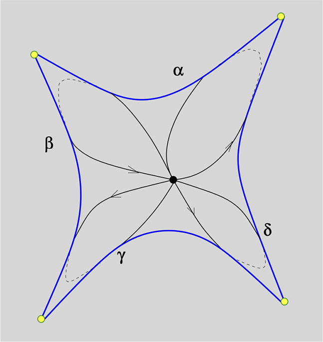
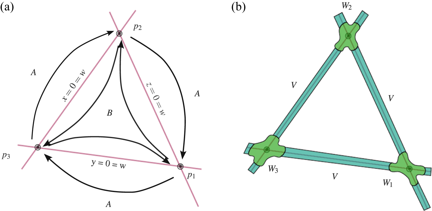


 Open access

