INTRODUCTION
In Mediterranean areas, factors such as climate, topography, soil characteristics, land use change and intensive agricultural practices have made soil erosion the main cause of land degradation (Cerdà Reference Cerdà2009; García-Ruíz & López-Bermúdez Reference García-Ruíz and López-Bermúdez2009). The Anoia-Penedès region, located in North-eastern Spain, provides a particularly good example of the effects of intensive erosion processes in Mediterranean Spain (Ramos & Martínez-Casasnovas Reference Ramos and Martínez-Casasnovas2010). In this region, the combination of frequent high-intensity rainfall events, highly erodible soil parent materials (marls and unconsolidated sandstones), extensive grapevine cropping, changes in land use and the abandonment of traditional soil conservation measures have contributed to the acceleration of erosion processes (Ramos & Martínez-Casasnovas Reference Ramos and Martínez-Casasnovas2007, Reference Ramos and Martínez-Casasnovas2010).
The need for clear and accurate estimations of soil erosion in agricultural areas is crucial for an understanding of the underlying processes and the development of prevention plans to reduce erosion (Casalí et al. Reference Casalí, Gastesi, Álvarez-Mozos, De Santisteban, Del Valle de Lersundi, Giménez, Larrañaga, Goñi, Agirre, Campo, López and Donézar2008). The scale of study and the assessment of land–climate interactions and their influences on soil erosion, water quality and agriculture are also issues that have captured the interest of many researchers, because their effects are seen off-site as well as on-site. On-site effects include soil, organic matter and nutrient losses, diminished infiltration and water availability, intra-field soil properties and crop variability, and the ultimate loss of soil fertility and crop production. Sediments and nutrients are exported, leading to reduced quality of water supplies and siltation of the drainage and irrigation systems (de Vente & Poesen Reference De Vente and Poesen2005).
Researchers have used different models to predict soil erosion and sediment transport and to assess the impact of management practices. Models to predict soil erosion include: (a) spatially distributed models, involving empirical (WaTEM-SEDEM – Van Rompaey et al. Reference Van Rompaey, Verstraeten, Van Oost, Govers and Poesen2001; Haregeweyn et al. Reference Haregeweyn, Poesen, Verstraeten, Govers, De Vente, Nyssen, Deckers and Moeyersons2013; USPED – Leh et al. Reference Leh, Bajwa and Chaubey2013) and physical approaches (PESERA – Kirkby et al. Reference Kirkby, Irvine, Jones and Govers2008; SWAT – Nearing et al. Reference Nearing, Jetten, Baffaut, Cerdan, Couturier, Hernandez, Le Bissonnais, Nichols, Nunes, Renschler, Souchère and Van Oost2005; Shen et al. Reference Shen, Gong, Li, Hong, Xu and Liu2009; Tibebe & Bewket Reference Tibebe and Bewket2011); (b) non-spatially distributed models, including regression and factorial models such as LMRM (Verstraeten & Poesen Reference Verstraeten and Poesen2001; Marquez & Guevara-Pérez Reference Marquez and Guevara-Pérez2010) R-USLE (Renard et al. Reference Renard, Foster, Weesies, McCool and Yoder1997; Grimm et al. Reference Grimm, Jones, Rusco and Montanarella2003) and PSIAC (de Vente & Poesen Reference De Vente and Poesen2005); and (c) conceptual models, such as AGNPS (Young et al. Reference Young, Onstad, Bosch and Anderson1989) and MMF (Morgan Reference Morgan2001). Other physically based models, such as EUROSEM (Morgan et al. Reference Morgan, Quinton, Smith, Govers, Poesen, Auerswald, Chisci, Torri and Styczen1998), WEPP (Flanagan et al. Reference Flanagan, Ascough Ii, Nearing, Laflen, Harmon and Doe2001; Shen et al. Reference Shen, Gong, Li, Hong, Xu and Liu2009), CREHDYS (Laloy & Bielders Reference Laloy and Bielders2009) and CREAMS (Knisel Reference Knisel1980) have also been applied extensively to cover a range of scales and environmental conditions. The selection of the model depends on the final objective, the data required to run and calibrate the model and the implicit uncertainty in interpreting the results obtained.
The Soil and Water Assessment Tool (SWAT) has been used widely to predict the impact of management practices on the yield of water, sediments and agricultural chemicals from basins at different scales (Gikas et al. Reference Gikas, Yiannakopoulou and Tsihrintzis2006; Lee et al. Reference Lee, Park, Park, Park, Lee and Kim2010; Martínez-Casasnovas et al. Reference Martínez-Casasnovas, Ramos and Benites 2013 ; Roebeling et al. Reference Roebeling, Rocha, Nunes, Fidelis, Aves and Fonseca2014). The SWAT model provides a powerful platform with which to analyse the influence of topography, soils, land cover, land management and weather in a spatially distributed way and to use the results to predict such parameters as runoff and sediment and nutrient losses.
Multiple applications of SWAT have been reported in the literature for different purposes. At present, SWAT is increasingly being used to assist watershed planning, with model applications becoming increasingly sophisticated in order to target critical pollutant source areas and practices. However, to date, applications in small basins have been limited (Bogena et al. Reference Bogena, Diekkrüger, Klingel, Jantos and Thein2003; Gevaert et al. Reference Gevaert, Van Griensven, Holvoet, Seuntjens and Vanrollegehm2008; Licciardello et al. Reference Licciardello, Rossi, Srinivasan, Zimbone and Barbagallo2011) and a few studies have focused on applications including detailed soil information. According to Mukundan et al. (Reference Mukundan, Radcliffe and Risse2010), the effect of spatial resolution on soil data may not be relevant in large watersheds; however, it may be determinant/pronounced in small ones and so it may be appropriate to formulate and simulate land-use management strategies.
The aim of the present research was to analyse the suitability of using SWAT in a small agricultural basin in the Mediterranean area, in which the local land and climatic characteristics tend to favour erosion. Given the absence of a gauging station in the study basin, soil water content data measured at different depths in the soil profile and runoff samples collected in various sub-basins were used for model calibration and validation. Another singular characteristic of the research was the great detail of the soil information used in the study and the land use: grape vines (Vitis vinifera), which were the main land use in the basin and there are very few cases of SWAT application with grape vines as a target crop.
MATERIALS AND METHODS
Study area
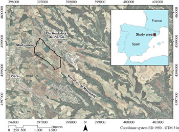
The study area was located in the municipality of Piera, c. 40 km Northwest of Barcelona (1°46′E, 41°31′N, 340 m a.s.l.) (Fig. 1). The main land use in the study area was grape vine cultivation, which has a long tradition in this area and belongs to the Penedès Designation of Origin. The study basin was selected according to the following criteria: small size (0·46 km2), the existence of a detailed soil map, the proximity to a meteorological station, and an area with non-irrigated vines as the main crop in the basin (0·629), which suffers severe erosion problems. The study area forms part of the Vallès-Penedès Tertiary Depression. The local soils developed on alluvial deposits dating from the Pleistocene Epoch, which covered a substratum of Miocene marls, sandstones and unconsolidated conglomerates. A high proportion of coarse elements of metamorphic origin were also present. The most frequent soils in the basin were classified as Typic Xerorthents, Fluventic Calcixerepts and Fluventic Haploxerepts (Soil Survey Staff 2006); or Haplic Regosols, Cutanic Luvisols, Haplic and Fluvic Cambisols (IUSS Working Group WRB 2006). The average slope in the basin was c. 9%. The basin drained into a gully system, which is characteristic of the landscape of the region in which the basin was located (Martínez-Casasnovas et al. Reference Martínez-Casasnovas, Ramos and García-Hernández2009).
(colour online) Location of the study basin in the municipality of Piera (Barcelona province, NE Spain).

In this area, deep ploughing (0·6–0·7 m) before the planting of vines is common in order to favour root penetration. Land levelling is also a frequent practice in order to create larger and more easily managed fields. This practice usually involves the abandonment of traditional soil conservation measures and the modification of soil profiles. Other studies conducted in this region have also reported important changes in soil properties after levelling operations (Ramos & Martínez-Casasnovas Reference Ramos and Martínez-Casasnovas2006), leading to the exposure of underlying marls, sandstones and conglomerates. Another associated problem is an increase in soil erosion, as reported by Martínez-Casasnovas et al. (Reference Martínez-Casasnovas, Ramos and García-Hernández2009), with a 26·5% increase in average annual soil loss associated with land transformation and the removal of traditional broad terraces.
The climate is Mediterranean, with average annual rainfall of 550 mm (ranging between 380 and 900 mm) and frequent high-intensity events in spring and autumn (>100 mm/h). The average annual rainfall erosivity (R factor=kinetic energy×maximum intensity in 30-min period) based on 1-min interval data is c. 1200 MJ/ha mm/h/year. However, in the decade 2000–10, some of these values ranged between 1350 and 3900 MJ/ha mm/h/year (Ramos & Martínez-Casasnovas Reference Ramos and Martínez-Casasnovas2009).
SWAT input data and measurements
The SWAT model simulates the hydrological water balance of the basin on the basis of hydrological response units (HRU), which are obtained from a combination of soil, land use and slope degree characteristics. The model operates on a daily time step. Flow and water quality variables are routed from the HRU to sub-basins and subsequently to the watershed outlet. The SWAT model simulates hydrological processes as a two-component system, comprised of surface hydrology and channel hydrology, as described by Neitsch et al. (Reference Neitsch, Arnold, Kiniry and Williams2011). It integrates various models: the Soil Conservation Service curve number technique (USDA-SCS 1985) is used to estimate runoff rates; the modified soil loss equation, MUSLE (Williams & Berndt Reference Williams and Berndt1977), is used for erosion and sediment yield at the catchment scale; and the routing of channel sediment is simulated through a modification of Bagnold's sediment transport equation (Bagnold Reference Bagnold1977).
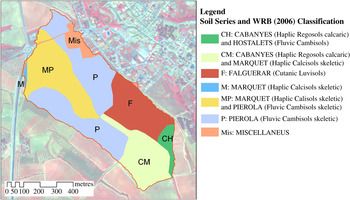
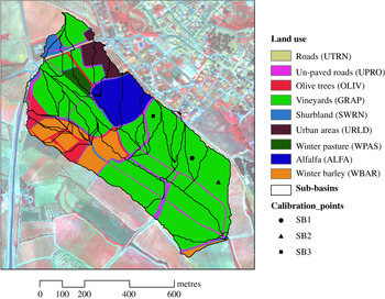
A detailed-scale soil map (1 : 25 000) (DAR 2008) was used as input data for the model. The soil information included in this map was detailed at the series level (Fig. 2). Additional soil information on relevant soil properties was obtained with a soil survey carried out in 2010. Forty sampling points located throughout the basin were selected; the locations of the samples were based on differences in the multi-spectral responses of soils which were seen in a false colour composite of a WorldView-2 image acquired in July 2010. Soil samples from 0 to 0·90 m (0–0·20, 0·20–0·50, 0·50–0·70 and 0·70–0·90 m) were taken at each point. Various soil properties were analysed, such as soil particle distribution (Gee & Bauder Reference Gee, Bauder, Klute, Campbell, Jackson, Mortland and Nielsen1986), bulk density (Pla Reference Pla1983), organic carbon (Allison Reference Allison, Black, Evans, Ensminger, White, Clark and Dinauer1965), electrical conductivity (Rhoades Reference Rhoades, Page, Miller, Keeney, Baker, Ellis and Rhoades1982) and water retention capacity at saturation, −33 and −1500 kPa, using Richard plates (Klute Reference Klute, Klute, Campbell, Jackson, Mortland and Nielsen1986). The coarse element fraction was evaluated in a 2-kg aliquot fraction which was sieved through a 2 mm mesh. The infiltration capacity was also analysed using rainfall simulation. The use of simulated rainfall to measure infiltration rates increases the accuracy of the measurements in comparison with the use of cylinder infiltrometers (Cerdà Reference Cerdà1997). The simulation was done in three sub-basins (SB1, SB2 and SB3), which corresponded to soils with different characteristics and located up-, mid- and down-slope (Fig. 3). The simulated rainfall consisted of 2·5-mm diameter drops of deionized water falling freely from drippers positioned 2·5 m above the soil surface. Plots of 0·30×0·20 m were subjected to 70 mm/h of simulated rainfall for 40 min. The runoff water was collected at 10-min intervals. Three replications were carried out at each sample point. The steady infiltration rate was reached in all cases after 30 min of rainfall. The intensity–frequency–duration used in the current study had a return period (or recurrence interval) in the area of 7 years, although during recent years the frequency of high-intensity rainfall events has been increasing. The eroded soil particles in suspension and the total runoff volume were measured for each simulation. Water infiltration rates were calculated from the difference between rainfall intensity and runoff rates. The rainfall intensity was calibrated just before and just after each simulation. In each sub-basin, the rainfall simulations were carried out in triplicate. The average value of the steady infiltration rate was used for further calibration of the model.
(colour online) Main soil series and classification according to World Reference Base (WRB 2006).

(colour online) Land use and the sub-basins as defined within the study basin. SB1, SB2 and SB3: sub-basins used for infiltration evaluations and model calibration and validation.

The soil erodibility factor (K USLE factor) was also computed for each soil unit, as this is input data for calculating SWAT: the equation proposed by Wischmeier et al. (Reference Wischmeier, Johnson and Cross1971) was used for this. The crop parameters were taken from the SWAT data base and updated with existing information for the study area relating to biomass phosphorus and nitrogen concentrations and crop fertilization and tillage operations for each land use.
A 1-m resolution digital elevation model (DEM) of the study area was also used for sub-basin delineation and slope degree calculation. The DEM was generated from a low-altitude photogrammetric aerial survey carried out in 2010. This permitted the computation of the degree of slope at the level of each grid. The following slope degree percentage intervals were considered 0–2, 2–5, 5–10, 10–15 and >15%. These intervals were established in relation to the signs of erosion observed in the field (no sign to slight, slight, moderate, severe and high erosion). They represented 0·05, 0·269, 0·508, 0·137 and 0·036 of the surface, respectively. These intervals of slope degree together with soil type and land used were used in the definition of the HRU. A land use map was created after orthorectification of the 2010 aerial photos at a scale of 1 : 3000 and field work checking. The ArcSWAT 2009.93.5 program was then run at a daily time scale.
Weather data were taken on a daily basis from the Els Hostalest de Pierola observatory, which belongs to the Servei Meteorològic de Catalunya (1°48′E; 41°31′N, 316 m a.s.l.) and was located 2·5 km away to the east of the study basin. Both daily data and average values for a 15-year series (1996–2011) of maximum and minimum temperatures, precipitation, solar radiation, relative humidity and wind velocity were used as inputs for the model. Precipitation was also recorded in the basin at 1-min intervals in order to determine rainfall intensity which was used, in combination with the steady infiltration rate, to estimate runoff rates.
The soil water content data for the profiles of the two sub-basins used for SWAT calibration were acquired using soil moisture sensors Decagon capacitance probes (TDF Decagon capacitance probes, Pullman, WA, USA). These probes were installed at different depths (0·10–0·30, 0·30–0·50, 0·50–0·70 and 0·70–0·90 m) in SB1 and SB2 (Fig. 3). Measurements were recorded every 4 h and then averaged to provide daily means. The probes were calibrated by comparison with soil water contents measured by gravimetry. Soil samples were taken at the same depths at which the TDF probes were installed at ten dates during the year in order to have information for a wide range of soil water contents. The correlation coefficients between gravimetric and volumetric soil water content were calculated for each date and probe: they ranged between 0·72 and 0·92. The correction factors, which ranged from 0·70 to 0·95, were averaged for each probe. With the corrected data obtained from the probes, depth-weighted volumetric water was estimated and then soil water storage in the profile was calculated.
Model calibration and validation
A sensitivity analysis was conducted using the SWAT sensitivity tool. It identified and ranked the sensitive parameters that affected the response of the model and the rate of change of its output with respect to changes in inputs. This analysis combines the Latin Hypercube and One-factor-At-a-Time sampling. During the sensitivity analysis, SWAT was run (p+1)×10 times, where p was the number of parameters being evaluated and 10 the number of loops. Different soil characteristics such as the saturated hydraulic conductivity, the soil depth and the soil available water capacity (AWC) were included in the analysis. Additional parameters such as the runoff curve number (CN2), the degree of slope, the surface runoff lag coefficient (SURLAG), the evaporation compensation factor (ESCO), the maximum potential leaf area index (BLAI) and the amount of water removed by transpiration from plants (Plant_ET), as well as parameters related to the groundwater such as the groundwater revap coefficient (which accounts for water movement into overlying unsaturated layers as a function of water demand for evapotranspiration, GW_revap), the threshold depth of water in the shallow aquifer required to return flow (GW_Qmin), the groundwater delay time (delay time or drainage time for aquifer recharge in days, GW_delay) and the base flow alpha factor (representing the ratio of base flow at the present time to the flow 1 day earlier, ranging from 0 to 1, Alpha_Bf), were included in the analysis of the hydrological response. For sediment production, the following parameters were included: Universal Soil Loss Equation Cover factor (USLE-C); soil conservation practices factor in the USLE equation (USLE-P); the sediment transport coefficient (SPCON); and the exponent in the sediment transport equation (SPEXP, ranging from 1 to 2). Additional explanations about the parameters and coefficients that were used can be found in Neitsch et al. (Reference Neitsch, Arnold, Kiniry and Williams2011).
The calibration was carried out by adjusting the selected parameters manually, one at a time, until the statistical calibration criteria were met. Calibration was carried out for the period 1 May 2010–30 April 2011, which included events with different characteristics (depth and intensity), as well as long dry periods and periods of high-intensity rainfall. The model was individually calibrated for SB1 and SB2, trying to fit the parameters in order to obtain the best results. The control parameters were: crop evapotranspiration (ETo), soil water content, runoff rates and soil loss due to runoff. Evapotranspiration was estimated in the SWAT using the Hargreaves equation (Hargreaves et al. Reference Hargreaves, Hargreaves and Riley1985). The ETo estimated by the model for the two sub-basins (planted with vines) was compared with the values calculated using the ETo obtained from the Els Hostalets de Pierola meteorological station and the crop coefficients proposed by Allen et al. (Reference Allen, Pereira, Raes and Smith1998). The soil evaporation compensation coefficient (ESCO), plant uptake compensation factor (EPCO) and Plant_ET coefficients (Neitsch et al. Reference Neitsch, Arnold, Kiniry and Williams2011) were adjusted to find the best fit between simulated and estimated ETo and soil moisture. Runoff rates, which were calculated taking into account steady infiltration rates and sealing and precedent soil moisture, were compared with the surface runoff simulated by the model. The comparison was carried out for the same sub-basins in which soil water probes were installed. Daily rainfall events with precipitation >9 mm, which some authors have identified as erosive rainfall (Mannaerts & Gabriels Reference Mannaerts and Gabriels2000), were also considered in a detailed rainfall analysis. Runoff samples were collected after the main rainfall events recorded during the calibration period using Gerlach troughs. The collectors were 0·5 m wide, with covered tops to prevent the entry of precipitation water. The Gerlach troughs were connected to underground collectors, hidden in the soil to collect runoff. After each rainfall event, total runoff was taken from the collectors using a vacuum pump, after homogenizing. After measuring the volume, these samples were analysed, in aliquots, for sediment concentration in runoff; the aliquots were dried at 105 °C for 24 h and then weighed. The results obtained were then used in conjunction with runoff water volumes to calculate soil losses for each runoff sampling point and compared with simulated soil losses. For each event the simulated runoff and soil loss integrated over time were compared with the estimated values.
Validation was carried out for the period 1 May 2011–15 May 2012. Field measurements for soil water content, rainfall and runoff were also recorded for that period. Model performance for both calibration and validation periods was defined based on three statistical methods: the Nash–Sutcliffe efficiency (NSE; Nash & Sutcliffe Reference Nash and Sutcliffe1970), the percent bias (PBIAS, %; Gupta et al. Reference Gupta, Sorooshian and Yapo1999) and the ratio of the root mean square error to standard deviation (RSR) (Eqns 1 to 3).
 $${\rm NSE} = 1 - \displaystyle{{\sum\nolimits_{i = 1}^n {(Y_{\rm m} - Y_{\rm s} )^2}} \over {\sum\nolimits_{i = 1}^n {(Y_{\rm m} - \bar Y)^2}}} $$
 $${\rm PBIAS} = \displaystyle{{\sum\nolimits_{i = 1}^n {(Y_{\rm m} - Y_{\rm s} )} \times 100} \over {\sum\nolimits_{i = 1}^n {(Y_{\rm m} )}}} $$
 $${\rm RSR} = \displaystyle{{\sqrt {\sum\nolimits_{i = 1}^n {(Y_{\rm m} - Y_{\rm s} )^2}}} \over {\sqrt {\sum\nolimits_{i = 1}^n {(Y_{\rm m} - \bar Y)^2}}}} $$
where Y
m is the measured value and Y
s is the simulated value with SWAT, and
 $\bar Y$
is the mean of the measured values of each of the parameters analysed.
RESULTS
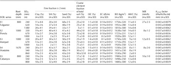
Table 1 presents a summary of the statistics of the soil properties of the study basin. Most of the soils had a loamy or a sandy-loam texture, with the average proportion of coarse elements ranging from 0·098 to 0·284 in the top horizon. The organic matter content was relatively low, ranging from 9 to 23 g/kg. The AWC ranged from 7·7 to 12·2 mm and the steady infiltration rate ranged from 8·0 to 29·5 mm/h. Some soils in the basin were very erodible, with K USLE factors ranging from 0·033 to 0·055 (t/ha/h)/(ha MJ mm). Soil depth ranged from 0·80 to 1·10 m, and none of the sampled soils showed any signs of (pseudo) gley phenomena, which indicated a good circulation of drainage water within the soil profile.
Mean values (m) and standard deviation (sd) of soil properties of the most representative soils in the study basin: root depth, lower boundary depth of each horizon (SDH), texture fraction (clay, silt, sand – USDA), coarse elements, organic carbon (OC), electrical conductivity (EC), bulk density (BD), available water capacity (AWC=water retention capacity at 33 kPa − water retention capacity at −1500 kPa), steady infiltration rate (StIR); K-erodibility USLE factor (K-factor)

Precipitation events and soil moisture dynamics
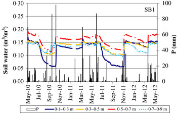
During the calibration period (1 May 2010–30 Apr 2011) rainfall events with different characteristics were recorded, with levels of daily precipitation ranging from <1 to 97·7 mm (Fig. 4). Twenty-three events recorded >9 mm of precipitation, which represented 0·833 of the total rainfall in the period. Precipitation was distributed throughout the year, but the main rainfall events were recorded in May, September and October 2010 and March 2011. Four events with precipitation >99% percentile were recorded. Total depths of those events were 69·7, 85·9, 97·7 and 69·6 mm, with 30-min rainfall intensities that were >50 mm/h and 10-min intensities of up to 120 mm/h.
(colour online) Daily precipitation (P) and volumetric soil water content (m3/m3) measured at different depths in the study sub-basin (SB1).

During the model validation period (1 May 2011–15 May 2012), 24 erosive events of different characteristics were recorded; these were mainly distributed in spring and autumn (Fig. 4). Precipitation ranged from 9·2 to 87·9 mm, including three extreme events of 69·6, 87·9 and 46·5 mm and with 30-min rainfall intensities of up to 37 mm/h. The precipitation recorded in these erosive events represented 0·852 of total rainfall and was mainly concentrated in October–November 2011 and March–April 2012, with a long dry period in between.
Figure 4 shows the variations in one of the control sub-basins (SB1) at four different soil depths. The soil water response after each rainfall event depended on the antecedent soil water content and on rainfall intensity. It was observed that soil water content changed in a different way in each soil layer. The greatest variations were observed in the surface layers, which could be explained by evaporation processes, particularly during dry periods. After high-intensity rainfall events, soil water increased in the surface layer but not in the deeper layers. Another notable aspect was that the highest soil water content was found in the layer between 0·50 and 0·70 m than in deeper layers, which could be due to the higher water retention capacity of the soil in that layer. This was found in most of the soils in the basin.
SWAT model application in the study basin
Land use and hydrological response units
Thirty-four sub-basins were identified within the study basin. Detailed spatial information about soil units, slope degree and land use allowed the definition of 1180 HRU in the sub-basins. The extensions of these HRU ranged from <0·01 to 1·39 ha, with 0·96 being<0·3 ha. Vines occupied 0·629 of the area: other crops present in the basin were: olive trees (0·048), alfalfa (0·085), winter barley (0·094), winter pasture (0·015) and scrub (0·036). Urban areas and (paved and un-paved) roads and tracks represented c. 0·093 of the total surface area (Fig. 3).
Sensitivity analysis
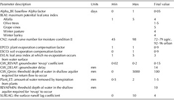
The sensitivity analysis results showed the most sensitive parameters that affected both the hydrological response and the sediment production: they were ranked on a scale from 0 to 33. The ones with rank >10 demonstrated variations in the SWAT output and were considered as sensitive parameters. Among them, soil characteristics such as the CN2, the saturated hydraulic conductivity, the soil depth and the AWC were the most sensitive parameters with regard to hydrological processes. The model was also sensitive to other parameters such as SURLAG, CN2, slope, ESCO, BLAI, Plant_ET, GW_revap, GW_Qmin, GW_delay and Alpha_Bf. For sediment production all parameters included in the analysis except the channel's resistance to erosion were sensitive. Despite the fact that some parameters, such as AWC, saturated hydraulic conductivity and soil depth or slope, were highlighted as sensitive parameters, the final values adopted were not modified since they were obtained from the specific field survey carried out for the present research. For those susceptible to change, a detailed sensitivity analysis was performed in order to know not only the influence on runoff but also on other components of the water balance. The adjusted parameters and their final values are shown in Table 2. The initial soil water conditions were also updated with measured data.
Parameter values used for modelling runoff and soil loss

Model calibration
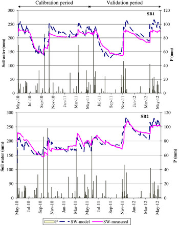
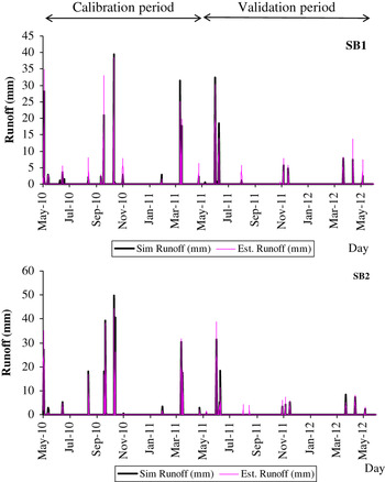
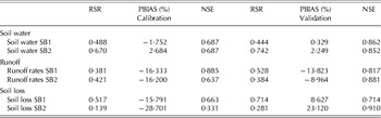
Soil water data measured in the field and soil water data simulated for SB1 and SB2 during the calibration period are shown in Fig. 5. The calibration statistics for soil water content are shown in Table 3: the calibration sample for soil water content included 327 days. There were differences between the basins, with the fit between simulated and measured data for SB2 being better than that for SB1. For the calibration period, the RSR statistics for the soil water content in the profile were 0·488 and 0·670, respectively for SB1 and SB2. The PBIAS were −1·752 and 2·684% and the NSE was 0·687 for both sub-basins. The statistics for runoff and soil loss calibration were based on 15 and 14 samples, respectively (Table 3). Simulated daily runoff rates and estimates obtained, taking into account steady infiltration rates based on the rainfall simulation and the antecedent soil water for both sub-basins, are shown in Fig. 6. The fit for runoff rates was slightly better for SB1 than for SB2 according to RSR, but not according to the other two statistics (PBIAS and NSE).
(colour online) Comparison between modelled and measured soil water in the soil profile in two sub-basins (SB1 and SB2) and daily precipitation (P).

(colour online) Comparison between estimated and simulated runoff for SB1 and SB2 for the calibration and validation periods.

Statistics of the comparisons between simulated and measured data during calibration and validation periods

Model validation
The statistics obtained for the validation period are also shown in Table 3. For soil water, the validation period included 245 days. The RSR were 0·444 and 0·742, the PBIAS were 0·328 and 2·249%, and the NSE were 0·862 and 0·852, respectively, for the SB1 and SB2 sub-basins. For the runoff and soil loss rates, the validation statistics referred to 14 days. For the runoff rates, RSR had values of 0·528 and 0·384, PBIAS of −13·823 and −8·964%, and NSE of 0·817 and 0·881, respectively, for the two sub-basins. Similarly, for soil loss, the validation results showed better fits for RSR and NSE than for PBIAS in SB2 and the opposite in SB1, with RSR values of 0·714 and 0·281, PBIAS values of 8·627 and 23·120% and NSE values of 0·714 and 0·910, respectively, for the two sub-basins. The runoff rates and soil losses predicted by the model were on average in agreement with the soil losses estimated by combining runoff rates and sediment concentrations in runoff. The greatest differences occurred with extreme rainfall events of high intensity and a short duration, which do not tend to be very well detected in a daily scale analysis. Among the two analysed sub-basins the greater discrepancies between simulated and estimated were found in the area where erosion was highest. During the analysed period, the average runoff rate in the basin was about 0·22, but with higher values for some specific sub-basins in which vines were cultivated and due to the combination of slope degree, soil characteristics and management practices (with bare soil throughout most of the years).
DISCUSSION
Calibration and validation
Following similar criteria to those provided by Moriasi et al. (Reference Moriasi, Arnold, Van Liew, Bingner, Harmel and Veith2007), the first calibration analysis for runoff and sediment could be considered satisfactory, particularly considering that the analysis was carried out using daily data. The NSE was of the same order as those observed by Narasimhan et al. (Reference Narasimhan, Srinivasan, Arnold and Di Luzio2005), and the RSR were similar to those observed by Li et al. (Reference Li, Ma and Du2010) for soil moisture analysis. The use of soil water content for model calibration and validation was useful because this is a parameter that can be measured at different points in the basin. This also means that it is possible to have additional information about water infiltration and soil response (infiltration and redistribution within the soil profile). In addition, antecedent soil moisture has been identified as one of the main factors that conditions runoff rates (Castillo et al. Reference Castillo, Gómez-Plaza and Martínez-Mena2003; Zhang et al. Reference Zhang, Wei and Nearing2011). This could be important for understanding when to apply runoff and soil erosion models in order to assess soil conditions and the effects of rainstorms, including soil erosion.
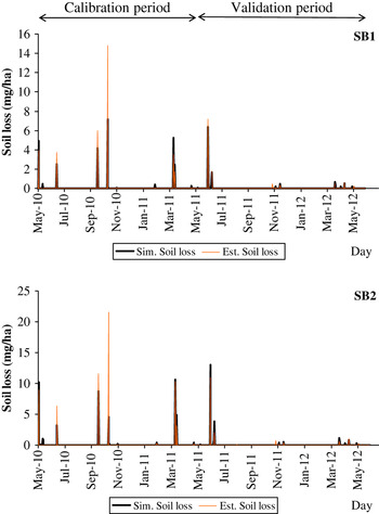
Although the soil loss results could be considered satisfactory for the control sub-basins, the agreement between simulated and measured soil loss was better for SB2 than for SB1, according to RSR and NSE, but was poorer according to PBIAS. By analysing the ratios between soil erosion and sediment yield (soil losses in the text) estimated by SWAT for these sub-basins, it was possible to observe that the poorer fits were associated with high-intensity precipitation events of a short duration (Fig. 7). This was the case of some of the events recorded in June (14, 16, 18 and 21) and September (8, 15 and 21) 2010 and in August (13) and November (10, 11, 17, 18 and 19) 2011. In addition, for the events in which the fit was good, sedimentation was very low or null. However, for higher intensity events for which higher erosion rates were expected, sedimentation was quite important, accounting for between 0·20 and 0·30 of soil losses. This might explain the differences between the amount of soil mobilized at some specific points and that modelled in the sub-basins.
(colour online) Comparison between estimated and simulated soil erosion for SB1 and SB2 for the calibration and validation periods.

For the validation period, there was no clear distinction in the fit between simulated and measured soil loss in one of the sub-basins and few differences were observed when they were compared with the values observed for calibration. Only PBIAS improved, slightly. The greatest discrepancies were found for short duration and high-intensity events.
From the current analysis, it can be concluded that the model gives a satisfactory fit for the hydrological components of the balance. The methodological approach for calibrating SWAT in small ungauged basins (i.e. where the water flow is not systematically measured in the basin by means of a water flow flume or similar equipment) and the use of detailed soil data allowed suitable runoff rates and reasonably good soil loss predictions to be obtained for most situations, but less satisfactory results were seen when extreme events or high-intensity, short duration, rainfall events occurred. This agrees with the poorer performance of other runoff and sediment yield predictions found in Mediterranean areas in predicting extreme peak flows (Licciardello et al. Reference Licciardello, Zema, Zimbone and Bingner2007). The characteristics of the rainfall events in the study area, which in many cases would have been of short duration and high intensity, would require exploring the possibilities of using sub-daily information as an input model parameter. However, despite this fact, the model could be a good tool to predict the hydrological processes. In addition, the model allowed the comparison of soil losses for years with different characteristics.
The agreement between results of the SWAT application in the present case study and with other works in the same and other areas with Mediterranean conditions suggests validity of the calibration method proposed for small ungauged basins. This methodological approach differs from that used in other works, in which the SWAT model has been mostly applied to large basins (Rossi et al. Reference Rossi, Srinivasan, Jirayoot, Le Duc, Souvannabouth, Binh and Gassman2009; Arnold et al. Reference Arnold, Allen, Volk, Williams and Bosch2010; Parajuli Reference Parajuli2011), for which water flow data in gauge stations is available.
The erosion rates obtained during the two calibration and validation periods were comparable to those estimated at plot scale for vines with similar management regimes in the same area (Ramos & Martínez-Casasnovas Reference Ramos and Martínez-Casasnovas2009). These values were always highest in the most disturbed areas of the new vineyards (Ramos & Martínez-Casasnovas Reference Ramos and Martínez-Casasnovas2007). Vineyards have been reported as one of the most erosion-prone types of cultivated land in Europe. At plot scale in the Mediterranean area, Cerdan et al. (Reference Cerdan, Govers, Le Bissonnais, Van Oost, Poesen, Saby, Gobin, Vacca, Quinton, Auerswald, Klik, Kwaad, Raclot, Ionita, Rejman, Rousseva, Muxart, Roxo and Dostal2010) reported a mean value of 8·64 t/ha/year as an average of different plots, with high variation (sd=27·4). The measured and simulated results obtained in the current analysis were comparable to these values and also similar to the maximum values reported by various authors in relation to arable land in other European countries, with values ranging from 10 to 20 t/ha/year (Verheijen et al. Reference Verheijen, Jones, Rickson and Smith2009) and simulated erosion rates for vineyards in other areas with Mediterranean climates (Potter & Hiatt Reference Potter and Hiatt2009). Thus, Bienes et al. (Reference Bienes, Marqués and Ruiz-Colmenero2012) indicated soil losses up to 20 t/ha/year in vineyards with traditional management. Similarly, for bare-soil vineyards, Maetens et al. (Reference Maetens, Vanmaercke, Poesen, Jankauskas, Jankauskien and Ionita2012) found soil losses of 10–20 t/ha/year. Other studies have cited higher erosion rates: up to 60 t/ha/year in Sicilian vineyards without soil cover (Novara et al. Reference Novara, Gristina, Saladino, Santoro and Cerdà2011), 35 t/ha/year in the Mid Aisne (France) (Wicherek Reference Wicherek1991) and 8–36 t/ha/year in the Languedoc region (France) (Paroissien et al. Reference Paroissien, Lagacherie and Le Bissonnais2010).
The measured and simulated soil losses exceed the soil loss tolerance rates established for Europe (0·3–1·4 t/ha/year) which depend on driving factors (Verheijen et al. Reference Verheijen, Jones, Rickson and Smith2009), but are also higher than the threshold values accepted for arable lands, which range from 9 t/ha/year (Singh et al. Reference Singh, Babu, Narain, Bhushan and Abrol1992) to 11·2 t/ha/year (Mannering Reference Mannering and Morgan1981). The following ranks of soil loss have been defined for soils: slight (0–5 t/ha/year), moderate (5–10 t/ha/year), high (10–20 t/ha/year), very high (20–40 t/ha/year), severe (40–80 t/ha/year) and very severe (>80 t/ha/year). According to this classification, the level of soil erosion in the study basin of the current work would be classified as high to very high.
Spatial soil loss distribution in the basin
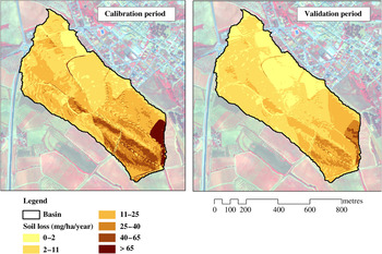
Due to the management practices used in the vines of the study basin, which include bare soil and frequent tillage throughout the crop cycle, high rates of erosion were expected. Within the basin, however, differences on parameters such as water runoff and sediment yield were found between sub-basins due to the combined influence of soil properties and slope degree. Figure 8 shows the spatially distributed simulated soil losses produced in the basin for both calibration and validation periods. The highest erosion rates were recorded near the outlet, where the slope degree is highest and the infiltration capacity of the soils is lowest. Furthermore, due to levelling operations undertaken before the vineyard plantation, the area was severely disturbed, with a great amount of unconsolidated material having been left on the surface.
(colour online) Soil erosion rate simulated within the basin during the calibration and validation periods.

In both periods (calibration and validation), but particularly during the first one, highly erosive rainfall events were recorded. Accordingly, high erosion rates were observed. During the calibration period, four events produced 0·87 of the total erosion. In this case, the differences between the simulated and estimated erosion rates were c. 23% in the SB1 sub-basin and up to 40% in the SB2 sub-basin. During the validation period, there was only one extreme event of similar characteristics (86·9 mm) to those recorded in the previous period and four additional events that produced erosion rates of greater than 0·2 t/ha. For that extreme event, the differences between the measured and estimated erosion rates were 12·1 and −16%, respectively, for the two areas. For the rest of the events, the differences were 17 and 30%, respectively, for SB1 and SB2. The results showed that the model simulations presented higher levels of variability, and with less agreement, in the zones located near the outlet, where the model produced higher erosion rates.
The SWAT allowed identification of the areas that suffer greater erosion. This is important in order to establish conservation measures in specific areas of the basin which could reduce soil erosion. This would not only result in a reduction in soil losses, but would also increase the amount of water available for agricultural needs.
This work is part of research project AGL2009-08353 funded by the Spanish Ministry of Science and Innovation. We would like to thank Dr R. Srinivasan for his help in setting up the model and helping to adapt its parameters to achieve a better fit for the study case. We would also like to thank the Castell d'Age winery for its support and for allowing us to carry out our field experiments on its property.